Abstract

We examine the equivalence between the Konishi anomaly equations and the matrix model loop equations in ${\cal N}=1^{*}$ gauge theories, the mass deformation of ${\cal N}=4$ supersymmetric Yang-Mills. We perform the superfunctional integral of two adjoint chiral superfields to obtain an effective ${\cal N}=1$ theory of the third adjoint chiral superfield. By choosing an appropriate holomorphic variation, the Konishi anomaly equations correctly reproduce the loop equations in the corresponding three-matrix model. We write down the field theory loop equations explicitly by using a noncommutative product of resolvents peculiar to ${\cal N}=1^{*}$ theories. The field theory resolvents are identified with those in the matrix model in the same manner as for the generic ${\cal N}=1$ gauge theories. We cover all the classical gauge groups. In $SO/Sp$ cases, both the one-loop holomorphic potential and the Konishi anomaly term involve twisting of index loops to change a one-loop oriented diagram to an unoriented diagram. The field theory loop equations for these cases show certain inhomogeneous terms suggesting the matrix model loop equations for the ${\bf RP}^{2}$ resolvent.

 

Email: taichi@newton.skku.ac.kr

1 Introduction

It was conjectured by Dijkgraaf and Vafa that the glueball superpotentials of a large class of ${\cal N}=1$ supersymmetric gauge theories are obtained by computing planar diagrams in certain bosonic matrix models [1, 2, 3]. The field theory proof of this conjecture was given in [3, 4] to show that the relevant contribution to the F-term comes from the planar diagrams with two gaugino insertions for each loop. In [4], they performed field theory perturbation by starting from the effective holomorphic action obtained by path integrating out all the anti-chiral superfields.

The reason why only planar diagrams are relevant to the F-term was clarified in [5] based on some properties of chiral operators. The chiral ring structure ensures that all the gauge invariant operators are equivalent to the operators with at most two gauge field insertions. Furthermore, the large $N$ factorization in the matrix model is simply the result of cluster decomposition of correlation functions of chiral operators. Then it was shown in [5] that the loop equations in a bosonic matrix model are reproduced as the Konishi anomaly equations induced by a certain holomorphic variation in the corresponding ${\cal N}=1$ gauge theory. In [5], the equivalence between the matrix model loop equations and the generalized Konishi anomaly equations was studied in an ${\cal N}=1$ theory with a polynomial superpotential for one adjoint matter field. The inclusion of fundamental matter fields was done in [7].

Meanwhile, in matrix model side there appeared some attempts to examine the conjecture in other kinds of ${\cal N}=1$ gauge theories. In [3], the matrix model computation of glueball superpotential was performed in the three-matrix model corresponding to the ${\cal N}=1^{*}$ gauge theories, the mass deformation of ${\cal N}=4$ super Yang-Mills. The peculiarity of ${\cal N}=1^{*}$ theories is that the theory contains three adjoint chiral superfields which interact through a commutator coupling. Since the tree-level superpotential is not simply a polynomial, the special geometry is implicit in the matrix model loop equations. As far as one intends to compute the glueball superpotential in perturbation expansion, one can treat the three adjoint fields equally and there is nothing different from a generic ${\cal N}=1$ theory with a polynomial superpotential [8]. However, to obtain the matrix model loop equations, one has to first integrate out two of three adjoint matrices to reduce the original three-matrix model into an effective one-matrix model. Then loop equations are derived as Schwinger-Dyson equations for the matrix model resolvents of a surviving matrix [3]. Motivated by the aforementioned works, it is natural to ask how the Konishi anomaly equations in ${\cal N}=1^{*}$ gauge theories reproduce the matrix model loop equations.

The string dual of ${\cal N}=1^{*}$ gauge theories was studied in [9]. The mass deformation in field theory corresponds to turning on a supergravity background in $AdS_{5}\times S^{5}$ compactification. Consequently, D3-branes polarize into a noncommutative sphere to form a dielectric D5-brane [9]. This situation is quite similar to the string theory setup of Dijkgraaf-Vafa conjecture. In a generic ${\cal N}=1$ theory equipped by a polynomial superpotential, D5-branes are wrapping around the blownup $S^{2}$’s obtained by resolving the conical singularities of a Calabi-Yau 3-fold described by the polynomial superpotential. In ${\cal N}=1^{*}$, the blownup $S^{2}$’s get replaced with fuzzy spheres resolving the $AdS_{5}$ singularity to yield the dielectric D5-branes.

In this paper, we derive the Konishi anomaly equations in ${\cal N}=1^{*}$ gauge theories. Instead of integrating out anti-chiral superfields [4], we first path integrate out two adjoint chiral superfields and their anti-chiral partners to gain an effective single adjoint theory. We also have corrections to the Kahler potential but these are irrelevant to the Konishi anomaly equations. Due to the ${\cal N}=1$ non-renormalization theorem, there is no perturbative corrections to the tree-level superpotential so that the lowest correction should include at least two spinor gauge superfields. Then using the chiral ring property, we will show the equivalence between the Konishi anomaly equations and the matrix model loop equations under an appropriate identification of matrix model resolvents in the field theory. We first derive the field theory loop equations in $U(N)$ gauge theories and check the consistency of results with [3]. The field theory loop equations are explicitly written down by using a noncommutative product of resolvents peculiar to ${\cal N}=1^{*}$ theories. Then we extend the results to cover $SO/Sp$ cases also. Especially, we extract the loop equation for the matrix model resolvent on ${\bf RP}^{2}$ out of the Konishi anomaly equations.

There are some remarks on the connection between the field theory perturbation and the matrix model perturbation. As noted in [10, 11], when we evaluate the glueball superpotential via matrix model perturbation, there arises a discrepancy between the matrix model and the field theory results beyond $h$-loops, with $h$ denoting the dual Coxeter number of the gauge group. This is due to the mixing ambiguities of chiral operators which have been discussed earlier in [12, 13]. In [14] they proposed one way to avoid these ambiguities through embedding the gauge group into a certain supergroup. However, the loop equations in matrix models are obtained by summing up all planar diagrams and we do not have to worry about the subtlety of order by order computation of planar diagrams. Instead, we have to identify the matrix model resolvents with those in the field theory. This was done in [15] in the generic ${\cal N}=1$ theories. The validity of this identification in ${\cal N}=1^{*}$ was suggested in [16]. In this paper, we will check the identification by deriving the field theory loop equations explicitly.

The organization of this paper is as follows. In section 2, we sketch the F-term computation of the one-loop effective theory, leaving the calculation details in appendix A. In section 3 we discuss Konishi anomaly equations in ${\cal N}=1^{*}$ and identify the field theory resolvents in the corresponding matrix model. The extension to $SO/Sp$ gauge groups is also discussed. Section 4 is devoted to conclusions and discussions.

Figure 1: Two ways to reduce a two adjoint theory to a single adjoint theory; (a) Integrating $\Phi$ field to obtain ${\rm Tr}\Psi^{4}$, (b) integrating $\Psi$ field to obtain ${\rm Tr}(W^{\alpha}\Phi^{2}){\rm Tr}W_{\alpha}$.

2 One-loop effective action in ${\cal N}=1^{*}$ gauge theories

2.1 The meaning of one-loop effective action

Let us start with the discussion of an ${\cal N}=1$ gauge theory with two adjoint chiral superfields. The tree-level superpotential is given by

$$W(\Phi,\Psi)={\rm Tr}(m\Phi^{2}+\Phi\Psi^{2})$$

as in footnote 1 in [5]. There are two ways to reduce this theory to a single adjoint theory. One is to integrate out $\Phi$ first. The only relevant diagram is the tree-diagram in figure 1 (a) and the theory turns out to be a single adjoint theory with the tree-level superpotential $W(\Psi)=-{\rm Tr}\Psi^{4}/4m$. The other is to integrate $\Psi$ first, then the effective theory is given by one-loop diagrams as in figure 1 (b). For each diagram not to vanish, it must contain at least two gauge field insertions as shown in the figure. This is consistent with the counting rule given in [4, 5], each loop has exactly two gluino insertions; two for one of two index loops or one for each index loop. Therefore starting from this effective theory, the Konishi anomaly equations seem to reproduce the matrix model loop equations. However, in this simplest case, we do not have to choose the latter way rather than manipulate the simple one-adjoint theory given in the former procedure.

The ${\cal N}=1^{*}$ theory contains three adjoint chiral superfields with three-point vertex involving a commutator of two adjoints. To gain the single adjoint theory, one must integrate out two of them and the situation is similar to the case (b). In the rest of this section, we will sketch the computation of the effective action in ${\cal N}=1^{*}$ gauge theories. For the details of computation, see appendix A.

2.2 Reduction to the ${\cal N}=1$ effective single adjoint theory

Using covariantly constrained chiral superfields, the lagrangian for an ${\cal N}=1^{*}$ gauge theory is written as

$${\cal L} = {1\over g^{2}}\Biggl{[}\int d^{4}\theta\;{\rm Tr}\left(\overline{\Phi}_{1}\Phi_{1}+\overline{\Phi}_{2}\Phi_{2}+\overline{\Phi}_{3}\Phi_{3}\right)+\int d^{2}\theta\,{1\over 2}\,W(\Phi)+\int d^{2}\bar{\theta}\,{1\over 2}\,\overline{W}(\overline{\Phi})\Biggr{]}$$ (2.1)

$$+{1\over 32\pi}{\rm Im}\left[\tau_{0}\int d^{2}\theta\;{\rm Tr}\,W^{\alpha}W_{\alpha}\right],$$

where the tree-level superpotential is given by

$$W(\Phi)={\rm Tr}\left[2\,\Phi_{3}\,[\Phi_{1},\Phi_{2}]+m\,(\Phi_{1}^{2}+\Phi_{2}^{2}+\Phi_{3}^{2})\right],$$ (2.2)

and $\tau_{0}$ is the bare Yang-Mills coupling

$$\tau_{0}={\theta\over 2\pi}+{4\pi i\over g^{2}}.$$

We will sketch our one-loop computation in $U(N)$ gauge groups. In $SO/Sp$ cases, the chiral superfields $\Phi_{i}$ can be either symmetric or antisymmetric tensor fields so that one has to insert appropriate projection operators to do trace calculation correctly. However this can be easily done through a small modification of $U(N)$ results.

In the lagrangian (2.1), $\Phi_{i}$ and $\overline{\Phi}_{i}$ are gauge covariant superfields subject to the constraints

$$\overline{\nabla}_{\dot{\alpha}}\Phi_{i}=0,\quad\nabla_{\alpha}\overline{\Phi}_{i}=0.$$

In the gauge chiral representation, they are related to the chiral superfields $\Psi_{i}$, $\overline{\Psi}_{i}$ via

$$\Phi_{i}=\Psi_{i},\quad\overline{\Phi}_{i}=e^{-{\rm ad}(V)}\overline{\Psi}_{i}\equiv e^{-V}\,\overline{\Psi}_{i}\,e^{V},$$

and accordingly the gauge covariant spinor derivatives are defined by [18]

$$\overline{\nabla}_{\dot{\alpha}}=\overline{D}_{\dot{\alpha}},\quad\nabla_{\alpha}=e^{-{\rm ad}(V)}D_{\alpha}e^{{\rm ad}(V)}\equiv{\rm ad}\!\left(e^{-V}D_{\alpha}e^{V}\right).$$

Note that in this representation $\Phi_{i}$ are ordinary chiral superfields eliminated by $\overline{D}_{\dot{\alpha}}$. The gauge field strength superfield $W_{\alpha}$ is defined by

$$W_{\alpha}=-{1\over 4}(\overline{D}^{2}e^{-V}D_{\alpha}e^{V}),$$

where the bracket means that the spinor derivatives are active only inside it.

Though the interaction involves a commutator of two adjoint superfields, it is still quadratic in $\Phi_{2}$ and $\Phi_{3}$ so that one can path integrate out $\Phi_{2}$, $\Phi_{3}$ and their anti-chiral partners to obtain the perturbatively exact effective action for an ${\cal N}=1$ gauge theory with a single adjoint field $\Phi\equiv\Phi_{1}$. Each diagram depends on the external gauge field in gauge covariant way through the covariant superfield propagators. It is further expanded into the diagrams with external gauge fields, namely $W_{\alpha}$’s, by using the Schwinger-Dyson equations for superfield propagators. One can easily compute the super-Feynman integrals by using the so-called covariant ‘D-algebra’ [18, 19]. Consequently, each of the one-loop diagrams reduces to a gauge-invariant non-local vertex among external $\Phi$ and $W_{\alpha}$ legs.

The most important point in the field theoretical proof of Dijkgraaf-Vafa conjecture might be the chiral ring property of chiral operators, i.e, the equivalence of gauge invariant operators modulo chiral rings. It ensures that the planarity of computation of the glueball superpotentials. As explained in [5], the correlation functions of gauge-invariant chiral operators are independent of the spatial coordinates and thereby factorized into a product of one-point functions due to the cluster decomposition of correlation functions. One can therefore reduce the nonlocal vertices of one-loop diagrams to a local holomorphic potential by extracting only the lowest order terms in the derivative expansion.

According to the ${\cal N}=1$ non-renormalization theorem, the terms corresponding to the one-loop diagrams without gauge field legs become trivially zero so that the non-trivial terms are those with at least two gauge field legs. Since, within the equivalence modulo chiral rings, $\Phi$ commutes with $W_{\alpha}$ and $W_{\alpha}$ obeys Fermi statistics, namely [5]

$$[\Phi,W_{\alpha}]=0,\quad\{W_{\alpha},W_{\beta}\}=0,$$

one may only compute the diagrams with two gauge field legs as well as even number of $\Phi$ legs to obtain the F-term of effective single adjoint theory. Therefore the lagrangian what we expect for the effective ${\cal N}=1$ theory can be written as

$${\cal L}_{\rm eff}=\int\!d^{4}\theta\,K(\overline{\Phi},\Phi)+\left[\int\!d^{2}\theta\,{1\over 2}\,\widetilde{W}(\Phi,W_{\alpha})+h.c.\right]+{1\over 32\pi}{\rm Im}\left[\tau_{0}\int d^{2}\theta\;{\rm Tr}\left(W^{\alpha}W_{\alpha}\right)\right].$$ (2.3)

Here we think of the theory as already renormalized, having all the one-loop corrections to the gauge coupling. The UV behavior of the theory is the same as ${\cal N}=4$ super Yang-Mills so that there is no one-loop correction to the gauge kinetic term at all. Although the Kahler potential contains one-loop corrections, they are irrelevant to the Konishi anomaly equations supposed the vacuum is supersymmetric.

2.3 Computation of one-loop holomorphic interactions

We are now led to compute the holomorphic $2n$-point function with $2n$ $\Phi$ fields as well as two spinor gauge fields. After some straightforward calculations, the full holomorphic corrections modulo chiral rings are summarized to be a holomorphic potential

$$\widetilde{W}(\Phi,W_{\alpha}) = {m\over g^{2}}{\rm Tr}\,\Phi^{2}+\sum_{n=1}^{\infty}\,{(-)^{n}\over n(2n+1)m^{2n}}\,W^{(2n)}(\Phi,W_{\alpha}),$$

$$W^{(2n)}(\Phi,W_{\alpha}) = W^{(0,2n)}(\Phi,W_{\alpha})+{1\over 2n}\sum_{r=1}^{2n-1}\sum_{s=1}^{2n-r}W^{(s,2n-s)}(\Phi,W_{\alpha}),$$ (2.4)

where $W^{(0,2n)}$ and $W^{(s,2n-s)}$ $(s=1,\dots,2n-1)$ are given by

$$W^{(0,2n)}(\Phi,W_{\alpha}) = {1\over 32\pi^{2}}{\rm Tr}_{\rm ad}\!\left[{\cal W}^{\alpha}{\cal W}_{\alpha}\phi^{2n}\right],$$

$$W^{(s,2n-s)}(\Phi,W_{\alpha}) = {1\over 32\pi^{2}}{\rm Tr}_{\rm ad}\!\left[{\cal W}^{\alpha}\phi^{s}{\cal W}_{\alpha}\phi^{2n-s}\right].$$ (2.5)

Here the traces are taken over the gauge adjoint representation. Note that there arises $\phi\equiv{\rm ad}(\Phi)$, instead of $\Phi$, inside the traces. They are rewritten as gauge fundamental traces of nested commutators;

$${\rm Tr}_{\rm ad}\!\left[{\cal W}^{\alpha}{\cal W}_{\alpha}\phi^{2n}\right] = {\rm Tr}\,\Bigl{[}e_{ji}\{W^{\alpha},[W_{\alpha},[\underbrace{\Phi,.....[\Phi}_{2n},e_{ij}]...]]\}\Bigr{]},$$

$${\rm Tr}_{\rm ad}\!\left[{\cal W}^{\alpha}\phi^{s}{\cal W}_{\alpha}\phi^{2n-s}\right] = {\rm Tr}\,\Bigl{[}e_{ji}\{W^{\alpha},[\underbrace{\Phi,.....[\Phi}_{s},[W_{\alpha},[\underbrace{\Phi,.....[\Phi}_{2n-s},e_{ij}]...]]]...]\}\Bigr{]},$$ (2.6)

where $(e_{ij})_{kl}=\delta_{ik}\delta_{jl}$ form a basis of gauge adjoint matrices to satisfy $X=e_{ij}X_{ij}$ for any gauge adjoint matrix $X$ whose $(i,j)$-component is $X_{ij}$. One can expand the nested commutators into operator products by using the identity;

$$[\underbrace{\Phi,.....[\Phi}_{n},X]...]=\sum_{r=0}^{n}\left({n\atop r}\right)(-)^{r}\,\Phi^{n-r}X\,\Phi^{r}.$$

Figure 2: The holomorphic 2-point functions with two insertions of external gauge fields. A cross (dot) denotes an external $\Phi$ ($W_{\alpha}$) leg inserted to either of two index loops. For instance, the diagram (d) corresponds to $-{\rm Tr}(\Phi^{2}W^{\alpha}){\rm Tr}\,W_{\alpha}$.

Eventually, the holomorphic functions are given by the summations of double traces each of which corresponds to a one-loop ribbon diagram with two index loops.

$$W^{(0,2n)}(\Phi,W_{\alpha})\! = \!{1\over 16\pi^{2}}\sum_{r=0}^{2n}\left({2n\atop r}\right)(-)^{r}$$

$$\Bigl{[}{\rm Tr}\,\Phi^{r}\,{\rm Tr}(\Phi^{2n-r}W^{2})-{\rm Tr}(\Phi^{r}W^{\alpha})\,{\rm Tr}(\Phi^{2n-r}W_{\alpha})\Bigr{]},$$

$$W^{(s,2n-s)}(\Phi,W_{\alpha})\! = \!{1\over 16\pi^{2}}\sum_{r=0}^{s}\sum_{p=0}^{2n-s}\left({s\atop r}\right)\left({2n-s\atop p}\right)(-)^{r+p}$$ (2.7)

$$\Bigl{[}{\rm Tr}\,\Phi^{r+p}\,{\rm Tr}(\Phi^{2n-r-p}W^{2})-{\rm Tr}(\Phi^{r+p}W^{\alpha})\,{\rm Tr}(\Phi^{2n-r-p}W_{\alpha})\Bigr{]}.$$

The binomial factors in the summations count the different ways to distribute $2n$ external $\Phi$ legs either on the inner index loop or on the outer index loop. The $\Phi$ legs on the same index loop commute with each other, while two $\Phi$ legs on different index loops are noncommutative. This is due to the commutator coupling in the original ${\cal N}=4$ super Yang-Mills. In figure 2, we showed the ribbon diagrams corresponding to the double traces in $W^{(0,2)}$. In the diagram (d), the inner index loop has one insertion of $W^{\alpha}$, while the outer index loop contains two $\Phi$ legs as well as $W_{\alpha}$ to yield the double trace of $-{\rm Tr}\,W^{\alpha}\,{\rm Tr}(\Phi^{2}W_{\alpha})$.

3 Konishi anomaly equations in ${\cal N}=1^{*}$ theories

3.1 Field theory resolvents and holomorphic interactions

We will see shortly that what one needs for evaluating the Konishi anomaly equations is the $\Phi$ derivative of the holomorphic function (2.4). In spite of the multi-summations in (2.4), they are summable by using the field theory resolvents, i.e, the generating functions for the gauge invariant chiral operators. Within the equivalence modulo chiral rings, all of those operators reduce to the three classes of operators;

$${\rm Tr}\,\Phi^{r},\quad{\rm Tr}(\Phi^{r}W_{\alpha}),\quad{\rm Tr}(\Phi^{r}W^{2}).$$

Thus we are led to introduce the field theory resolvents;

$$R(z) \equiv {\rm Tr}\,\widehat{R}(z)\;=\;-{1\over 32\pi^{2}}{\rm Tr}\,W^{2}\,{1\over z-\Phi},$$

$$w_{\alpha}(z) \equiv {\rm Tr}\,\widehat{w}_{\alpha}(z)\;=\;{1\over 4\pi}{\rm Tr}\,W_{\alpha}\,{1\over z-\Phi},$$

$$T(z) \equiv {\rm Tr}\,\widehat{T}(z)\;=\;{\rm Tr}\,{1\over z-\Phi}.$$ (3.1)

Suppose that $\Phi$ has some continuous distributions of its eigenvalues around the classical vacua. Then by choosing the counter $\cal C$ on the complex $z$-plane such that it encircles the branch cuts of eigenvalue distributions, the gauge invariant chiral operators are given by the contour integrals of field theory resolvents;

$${\rm Tr}(\Phi^{r}W^{2}) = \oint_{\cal C}{dz\over 2\pi i}\,z^{r}R(z),$$

$${\rm Tr}(\Phi^{r}W_{\alpha}) = \oint_{\cal C}{dz\over 2\pi i}\,z^{r}w_{\alpha}(z),$$

$${\rm Tr}\,\Phi^{r} = \oint_{\cal C}{dz\over 2\pi i}\,z^{r}T(z).$$ (3.2)

These formulas convert the power of $\Phi$ into the power of $z$ free from the traces of resolvents and make the summations involving binomial coefficients doable.

Consequently, we arrive at a rather simple result;

$${\partial\over\partial\Phi}W^{(s,2n-s)}(\Phi,W_{\alpha})=4n\oint_{\cal C}{dz\over 2\pi i}\,(z-\Phi)^{2n-1}\left[R(z)+w^{\alpha}(z)\widehat{v}_{\alpha}+T(z)\widehat{S}\right],$$

for $s=0,1,\dots,2n-1$. Here we have introduced the chiral operators

$$\widehat{S}\equiv-{1\over 32\pi^{2}}W^{2},\quad\widehat{v}_{\alpha}\equiv{1\over 4\pi}W_{\alpha}.$$

Note that we attach a hat symbol to a gauge covariant chiral operator whose trace yields the corresponding gauge singlet chiral field or the field theory resolvent. Together with the factor $4n$ above, the summations in the second equation of (2.4) provide a factor $2n(2n+1)$ and cancels the prefactor $1/n(2n+1)$ in the first equation of (2.4). Finally the $\Phi$ derivative of $\widetilde{W}(\Phi,W_{\alpha})$ is determined as

$$\widetilde{W}^{\,\prime}(\Phi,W_{\alpha}) = {2m\over g^{2}}\Phi-\oint_{\cal C}{dz\over 2\pi i}\left[{1\over z-\Phi+im}+{1\over z-\Phi-im}\right]$$ (3.3)

$$\;\left[R(z)+w^{\alpha}(z)\widehat{v}_{\alpha}+T(z)\widehat{S}\right].$$

3.2 Konishi anomaly as the field theory loop equations

The Konishi anomaly equations are obtained as anomalous Ward-Takahashi identities associated with an arbitrary holomorphic variation $\delta\Phi=f(\Phi,W_{\alpha})$, while keeping $\overline{\Phi}$ unchanged, in the effective single adjoint theory (2.3). Specifically, they are given as an identity

$$0=\int\!d^{8}z^{\prime}\!\int\,[d\overline{\Phi}][d\Phi]\;{\rm Tr}_{\rm ad}\left[{\partial\over\partial\Phi(z^{\prime})}f(\Phi(z),W_{\alpha}(z))\exp\left(i\!\int\!d^{4}x\,{\cal L}_{\rm eff}\right)\right],$$

where the trace must be an adjoint trace since inside the square brackets is a matrix in the gauge adjoint representation. Thus we obtain the generalized Konishi anomaly

$$-{1\over 4}\overline{D}^{2}\langle J_{f}\rangle=i\left\langle\int\!d^{8}z^{\prime}\,{\rm Tr}_{\rm ad}\left[{\partial f(\Phi(z),W_{\alpha}(z))\over\partial\Phi(z^{\prime})}\right]\right\rangle-{1\over 2}\left\langle{\rm Tr}\left[f(\Phi,W_{\alpha})\widetilde{W}^{\,\prime}(\Phi,W_{\alpha})\right]\right\rangle.$$ (3.4)

The current $J_{f}$ is induced by the holomorphic variation of the Kahler potential and is given by

$$J_{f}={\rm Tr}\left[\frac{\partial K(\overline{\Phi},\Phi)}{\partial\Phi}f(\Phi,W_{\alpha})\right].$$ (3.5)

Now the Kahler potential might include the one-loop corrections with external $\Phi$ and $\overline{\Phi}$ legs. However, on the supersymmetric vacuum, $\overline{D}^{2}\langle J_{f}\rangle=0$ and the only D-term contributions through $J_{f}$ to the Konishi anomaly simply vanishes [5]. Therefore we do not have to compute the D-term corrections. The anomaly term in (3.4) can be calculated by inserting the regulator function $\exp(-L)$ with $L=\overline{D}^{2}e^{-{\rm ad}(V)}D^{2}e^{{\rm ad}(V)}$. In our notation, the anomaly coefficient is $1/64\pi^{2}$ [20] and (3.4) goes to

$$-{1\over 32\pi^{2}}\left\langle{\rm Tr}\left[e_{ij}\left\{W^{\alpha},\left[W_{\alpha},\frac{\partial f(\Phi,W_{\alpha})}{\partial\Phi_{ij}}\right]\right\}\right]\right\rangle=\left\langle{\rm Tr}\left[f(\Phi,W_{\alpha})\widetilde{W}^{\,\prime}(\Phi,W_{\alpha})\right]\right\rangle,$$ (3.6)

which is the same as the generalized Konishi anomaly in [5] defining the glueball superfield $S$ to have the numerical factor $1/32\pi^{2}$. This is the reason why we inserted the factor $1/2$ in front of the superpotential.

In order to obtain the Konishi anomaly equations as the field theory loop equations comparable to those in matrix models, we choose the holomorphic variation as the form suggested by the matrix model resolvents, namely

$$f(\Phi,W_{\alpha})=\widehat{\cal R}(z)\equiv\widehat{\cal S}{1\over z-\Phi},$$ (3.7)

where as performed in [5] we have introduced the ${\cal N}=2$ glueball operator

$$\widehat{\cal S}\equiv\widehat{S}+\psi^{\alpha}\widehat{v}_{\alpha}-{1\over 2}\psi^{\alpha}\psi_{\alpha}\widehat{1}.$$

The hidden ${\cal N}=2$ supersymmetry is implemented by the fermionic coordinates $\psi_{\alpha}$. Note that the operator $\widehat{\cal R}(z)$ is decomposed into the ${\cal N}=1$ operators like

$$\widehat{\cal R}(z)=\widehat{R}(z)+\psi^{\alpha}\widehat{w}_{\alpha}(z)-{1\over 2}\psi^{\alpha}\psi_{\alpha}\widehat{T}(z),$$

and therefore the combination of the resolvents in (3.3) can be rewritten as

$$R(z)+w^{\alpha}(z)\widehat{v}_{\alpha}+T(z)\widehat{S}=-2\int\!d^{2}\psi\,{\cal R}(z)\,\widehat{\cal S}.$$ (3.8)

This ensures that the ${\cal N}=2$ language introduced in [5] to describe the field theory prepotential is still available in ${\cal N}=1^{*}$ gauge theories.

Substituting the special variation (3.7) into (3.4), the generalized Konishi anomaly turns out to be

$${\cal R}(z)^{2}={\rm Tr}\left[\widetilde{W}^{\,\prime}\widehat{\cal R}(z)\right],$$ (3.9)

which can be further decomposed into three equations for the three resolvents;

$$R(z)^{2} = {\rm Tr}\left[\widetilde{W}^{\,\prime}\widehat{R}(z)\right],$$

$$2R(z)w_{\alpha}(z) = {\rm Tr}\left[\widetilde{W}^{\,\prime}\widehat{w}_{\alpha}(z)\right],$$

$$2R(z)T(z)+w^{\alpha}(z)w_{\alpha}(z) = {\rm Tr}\left[\widetilde{W}^{\,\prime}\,\widehat{T}(z)\right].$$ (3.10)

Here we have used the factorization property of chiral operator correlation functions and suppressed the bracket symbols of field theory vevs. The formal expressions of the field theory loop equations (3.10) are the same as those for the ordinary ${\cal N}=1$ theory with a polynomial superpotential. The right hand side of (3.10) seems rather complicated because $\widetilde{W}^{\,\prime}(\Phi,W_{\alpha})$ involves all the field theory resolvents through the combination of (3.8). However, the loop equations are further simplified by virtue of the chiral ring properties;

$$\widehat{S}^{2}=0,\quad\widehat{S}\,\widehat{v}_{\alpha}=0.$$

It is straightforward by using this chiral ring properties to write down the Konishi anomaly equations (3.10) explicitly in the field theory resolvents.

$$R(z)^{2} = (R\circ R)(z)+[V^{\,\prime}R(z)]_{-}$$

$$2R(z)w_{\alpha}(z) = (R\circ w_{\alpha})(z)+(w_{\alpha}\circ R)(z)+[V^{\,\prime}w_{\alpha}(z)]_{-},$$ (3.11)

$$2R(z)T(z)+w^{\alpha}(z)w_{\alpha}(z) = (R\circ T)(z)+(w^{\alpha}\circ w_{\alpha})(z)+(T\circ R)(z)+[V^{\,\prime}\,T(z)]_{-},$$

where we have defined a noncommutative product $(O_{1}\circ O_{2})$ between two arbitrary functions $O_{1}$, $O_{2}$ by

$$(O_{1}\circ O_{2})(x)\equiv\oint_{\cal C}{dz\over 2\pi i}\left[{O_{1}(z+i)-O_{1}(x)\over z-x+i}+c.c.\right]O_{2}(z).$$ (3.12)

We also have replaced the mass deformation $\Phi^{2}$ with a polynomial superpotential $V(\Phi)$. $[V^{\,\prime}R(z)]_{-}$ means to drop non-negative powers in the Laurent expansion of $V^{\,\prime}(z)R(z)$ [5]. Here to compare our field theory results with the matrix model results in [3], we have rescaled all the superfields to be dimensionless;

$$\Phi\to m\Phi,\quad W_{\alpha}\to{m^{3/2}\over g}W_{\alpha},\quad\psi_{\alpha}\to{m^{3/2}\over g}\psi_{\alpha}.$$

This rescaling amounts to make the resolvents to scale correctly and yields (3.11).

We notice that the first equation is closed with respect to $R(x)$ and is equivalent to the matrix model loop equation through identification of $R(x)$ as the resolvent on 2-sphere. To further simply the equations, we now introduce the spectral decompositions

$$R(z) = \int_{-a}^{a}d\lambda\,\rho(\lambda)\,{1\over z-\lambda},$$

$$w_{\alpha}(z) = \int_{-a}^{a}d\lambda\,\rho(\lambda)u_{\alpha}(\lambda)\,{1\over z-\lambda},$$

$$T(z) = \int_{-a}^{a}d\lambda\,\rho(\lambda)c(\lambda)\,{1\over z-\lambda},$$ (3.13)

supposed that the gauge symmetry is unbroken and the eigenvalues of the resolvents are distributed along a single branch cut on the complex $z$-plane. The spectral densities obey the constraints given by the contour integrals of resolvents. By setting $r=0$ in (3.2) and applying the spectral decompositions above, they are written as

$$\int_{-a}^{a}d\lambda\,\rho(\lambda)=S,\quad\int_{-a}^{a}d\lambda\,\rho(\lambda)u_{\alpha}(\lambda)=v_{\alpha},\quad\int_{-a}^{a}d\lambda\,\rho(\lambda)c(\lambda)=N.$$

By using (3.13) in (3.11), the Konishi anomaly equations provide the following conditions for the resolvents along the branch cut $z\in(-a,a)$;

$$2R(z) = V^{\prime}(z)+R(z+i)+R(z-i),$$

$$2w^{\alpha}(z) = w^{\alpha}(z+i)+w^{\alpha}(z-i),$$

$$2T(z) = T(z+i)+T(z-i),$$ (3.14)

These equations fix the analytic properties of resolvents and uniquely determine the corresponding elliptic curve of a Riemann surface. The first equation reproduces the matrix model result in [3, 21] with $V^{\prime}(z)=2z$. It is an equation of motion for a probe matrix eigenvalue $z$. The mass deformation of ${\cal N}=1^{*}$ has been generalized to an arbitrary polynomial potential $V(\Phi)$ and the corresponding matrix model loop equation was analyzed in [10, 22]. It is exactly the first equation in (3.14) with $V^{\prime}(z)$ generalizing the mass deformation $2z$ of the original ${\cal N}=1^{*}$ theory.

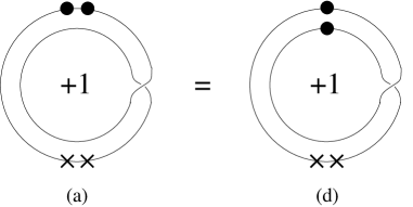
Figure 3: The double trace diagrams in figure 2 transfer to single trace diagrams due to the twisted part of $SO/Sp$ projection operator. The diagrams (a), (d) in figure 2 turn out to be the same single trace diagram of ${\rm Tr}(W^{2}\Phi^{2})$.

3.3 The field theory loop equations in $SO/Sp$ cases

The extension to $SO/Sp$ cases is straightforward as worked out in [15, 23, 24, 25, 26]. We do not have to repeat the computation of one-loop effective action performed in $U(N)$ except for the last step to calculate the adjoint traces in (2.6). In $SO/Sp$ groups, there exist two-index tensor fields $\Phi_{ij}$ either symmetric or antisymmetric under $i\leftrightarrow j$. Now the field $\Phi$ does not distinguish two index lines of a one-loop ribbon diagram and induces twisted diagrams like in figure 3. These diagrams cause a bit modification of the holomorphic potential $\widetilde{W}(\Phi,W_{\alpha})$. Accordingly, the Konishi anomaly equations are changed to involve the unoriented geometry of an ${\bf RP}^{2}$ Riemann surface.

To see this in more detail, let us introduce the projection operator [25, 15]

$$(P_{ij})_{kl}\equiv P_{ij,kl}={1\over 2}\left(\delta_{ik}\delta_{jl}+\sigma t_{il}t_{jk}\right),$$ (3.15)

where $t_{ij}$ denotes the invariant tensors for $SO/Sp$ groups, namely

$$t_{ij}=\delta_{ij},\quad\sigma=-1,\quad\mbox{$SO$ antisymmetric ($SO^{-}$)},$$

$$t_{ij}=\delta_{ij},\quad\sigma=+1,\quad\mbox{$SO$ symmetric ($SO^{+}$)},$$

$$t_{ij}=J_{ij},\quad\sigma=-1,\quad\mbox{$Sp$ symmetric ($Sp^{-}$)},$$

$$t_{ij}=J_{ij},\quad\sigma=+1,\quad\mbox{$Sp$ antisymmetric ($Sp^{+}$)},$$ (3.16)

where $J_{ij}$ is a symplectic tensor satisfying $J^{T}=-J$, $J^{2}=-\widehat{1}$. The tensor superfield $\Phi$ obeys the projection $\Phi_{ij}={\rm Tr}(P_{ji}\Phi)$ so that $P_{ij}$ plays the same role as $e_{ij}$ for $U(N)$ groups. The only change in the one-loop calculation is to replace $e_{ij}$ in (2.6) with $P_{ij}$.

The untwisted part of $P_{ij}$ does not cause any change in (2.7) except for the numerical factor 1/2. The twisted part causes an interchange of two indices and a double trace of two index loops turns out to be a single trace of one index loop. The twisting of indices also transposes the operators on one of two index loops. This yields an overall minus sign to the second term in (2.7). Accordingly, for the twisted sector the first and the second terms give the same single trace modulo chiral ring equivalence.

In figure 3 we demonstrated how twisting occurs in the simplest case of $W^{(0,2)}$. For the untwisted sector, we have (a) $+{\rm Tr}(W^{2}\Phi^{2})\,{\rm Tr}\,\widehat{1}$ and (d) $-{\rm Tr}(W_{\alpha}\Phi^{2})\,{\rm Tr}\,W^{\alpha}$. For the twisted sector, by using $\Phi^{T}=\sigma\,t\,\Phi\,t^{-1}$ and $W_{\alpha}^{T}=-t\,W_{\alpha}\,t^{-1}$, we can see that (a) and (d) transfer to the same single trace;

$$+{\rm Tr}(W^{2}\Phi^{2})\,{\rm Tr}\,\widehat{1} \to +\sigma{\rm Tr}\left[t\,(W^{2}\Phi^{2})^{T}\,t\,\widehat{1}\right]\;=\;\pm\sigma\,{\rm Tr}(W^{2}\Phi^{2}),$$

$$-{\rm Tr}(W^{\alpha}\Phi^{2})\,{\rm Tr}\,W_{\alpha} \to -\sigma{\rm Tr}\left[t\,(W^{\alpha}\Phi^{2})^{T}t\,W_{\alpha}\right]\;=\;\pm\sigma\,{\rm Tr}(W^{2}\Phi^{2}),$$

where the upper/lower sign for $SO/Sp$ groups. Things are the same for the other pairs of (b), (e) and (c), (f) to yield the twisted half of $W^{(0,2)}$ as $\mp 2\sigma(1-\sigma)^{2}\,{\rm Tr}(\widehat{S}\Phi^{2})$. Similarly one can evaluate the twisted half of $W^{(s,2n-s)}$. Since twisting reduces a double trace to a single trace, the twisted half has no dependence on $s$ to become $\mp 2\sigma(1-\sigma)^{2n}\,{\rm Tr}(\widehat{S}\Phi^{2n})$. The holomorphic potential $\widetilde{W}$ splits into untwisted and twisted parts; $\widetilde{W}=\widetilde{W}_{un}+\widetilde{W}_{tw}$. Their $\Phi$-derivatives are given by

$$\widetilde{W}^{\,\prime}_{un} = 2\Phi-{1\over 2}\oint_{\cal C}\frac{dz}{2\pi i}\left[{1\over z-\Phi+i}+{1\over z-\Phi+i}\right]\left[R(z)+w^{\alpha}(z)\widehat{v}_{\alpha}+T(z)\widehat{S}\right],$$

$$\widetilde{W}_{tw}^{\,\prime} = \pm\sigma(1-\sigma)\,\widehat{S}\left[{1\over 2\Phi+i}+{1\over 2\Phi-i}\right].$$ (3.17)

Note that the twisted potential exists only for $\sigma=-1$.

The anomaly term in (3.6) shares the same one-loop structure as the holomorphic potential $\widetilde{W}$ so that the same modification is necessary to gain the correct $SO/Sp$ loop equations. Again, we replace $e_{ij}$ with $P_{ij}$ so that $P_{ij}$ acts on both $\delta\Phi_{kl}=f(\Phi,W_{\alpha})_{kl}$ and $\partial/\partial\Phi_{ij}$. This modification was worked out in [15]. The results are

$${\rm Tr}\left[\widetilde{W}^{\,\prime}\widehat{R}(z)\right] = {1\over 2}\,R(z)^{2},$$

$${\rm Tr}\left[\widetilde{W}^{\,\prime}\,\widehat{T}(z)\right] = \left\{\begin{array}[]{ll}\left(T(z)-\frac{2}{z}\right)R(z)&\quad SO^{-},\\[8.0pt] \left(T(z)-2\frac{d}{dz}\right)R(z)&\quad SO^{+},\\[8.0pt] \left(T(z)+\frac{2}{z}\right)R(z)&\quad Sp^{-},\\[8.0pt] \left(T(z)+2\frac{d}{dz}\right)R(z)&\quad Sp^{+},\end{array}\right.$$ (3.22)

For $SO/Sp$ groups one can prove $w_{\alpha}(z)\equiv 0$ by using chiral ring properties [15]. In ${\cal N}=1^{*}$ $SO/Sp$ theories, the holomorphic potential $\widetilde{W}$ also receives the corrections we figured out.

Since $\widetilde{W}_{tw}^{\,\prime}$ is proportional to $\widehat{S}$, this is irrelevant in the first equation in (3.22), i.e,

$${\rm Tr}\left[\widetilde{W}_{un}^{\,\prime}\widehat{R}(z)\right]={1\over 2}\,R(z)^{2}.$$ (3.23)

In the second equation, $\widetilde{W}_{tw}^{\,\prime}$ provides inhomogeneous corrections for $SO^{-}/Sp^{-}$ to yield

$${\rm Tr}\left[\widetilde{W}_{un}^{\,\prime}\,\widehat{T}(z)\right]=\left\{\begin{array}[]{ll}\left[T(z)-2\left({1\over z}-{1\over 2z+i}-{1\over 2z-i}\right)\right]R(z)-\xi(z)&\quad SO^{-},\\[8.0pt] \left(T(z)-2{d\over dz}\right)R(z)&\quad SO^{+},\\[8.0pt] \left[T(z)+2\left({1\over z}-{1\over 2z+i}-{1\over 2z-i}\right)\right]R(z)+\xi(z)&\quad Sp^{-},\\[8.0pt] \left(T(z)+2{d\over dz}\right)R(z)&\quad Sp^{+},\end{array}\right.$$ (3.24)

where $\xi(z)$ is defined by

$$\xi(z)\equiv\frac{R(-{i\over 2})}{z+{i\over 2}}+\frac{R(+{i\over 2})}{z-{i\over 2}}.$$ (3.25)

The inhomogeneous corrections due to twisting reflect the informations of the matrix model resolvent defined on the ${\bf RP^{2}}$ Riemann surface.

3.4 Connection to the matrix model loop equations

The connection between the resolvents in field theories and those in matrix models was discussed in [15]. Now in (3.11) the first equation is closed by itself and coincides with the matrix model loop equation through the identification

$$R(z)={\bf R}_{S^{2}}(z),$$ (3.26)

with the matrix model resolvent defined on a Riemann surface of $S^{2}$ (two-sphere). This identification can be understood as follows. Following [1, 2, 15], we define the matrix model resolvent ${\bf R}_{S^{2}}(z)$ as

$${\bf R}_{S^{2}}(z)={\bf g}\left\langle{\rm Tr}\,{1\over z-{\bf\Phi}}\right\rangle$$

with the matrix model coupling constant ${\bf g}$. The planar diagrams contributing to the glueball superpotential are the leading order terms in the $1/N$ expansion of matrix model free energy with the finite ‘t Hooft coupling ${\bf S}={\bf g}N$. Then the prefactor ${\bf g}$ in the matrix model resolvent is actually ${\bf S}/N$ so that the identification $S={\bf S}$ of glueball superfield leads us to (3.26).

According to [15], the other two resolvents are given by ${\bf R}_{S^{2}}(z)$ as follows.

$$w_{\alpha}(z) = v_{\alpha}{\partial\over\partial{\bf S}}{\bf R}_{S^{2}}(z),$$

$$T(z) = N{\partial\over\partial{\bf S}}{\bf R}_{S^{2}}(z)+{v^{\alpha}v_{\alpha}\over 2}{\partial^{2}\over\partial{\bf S}^{2}}{\bf R}_{S^{2}}(z).$$ (3.27)

This identification is obvious in (3.11). One can see that the second and third equations in (3.11) are satisfied by the identification above because the ${\bf S}$ dependence of the first equation is only through the resolvent $R(z)$. The identification in ${\cal N}=1^{*}$ theories was also examined in [16] and is consistent with [15].

For $SO/Sp$ gauge groups, the planar diagrams of adjoint loops involve unoriented Riemann surfaces of ${\bf RP}^{2}$. The matrix model loop equations therefore include the resolvent ${\bf R}_{RP^{2}}(z)$ defined on the geometry of ${\bf RP}^{2}$. According to [15], the field theory resolvents are identified as follows.

$$R(z) = {\bf R}_{S^{2}}(z),$$

$$T(z) = N{\partial\over\partial{\bf S}}{\bf R}_{S^{2}}(z)+4\,{\bf R}_{RP^{2}}(z).$$ (3.28)

Obviously, the first term in $T(z)$ satisfies the homogeneous part of (3.24) so that the source of the inhomogeneity is nothing but the resolvent ${\bf R}_{RP^{2}}(z)$. This lead us to predict that the matrix model loop equation for ${\bf R}_{RP^{2}}(z)$ might be written as

$$({\bf R}_{S^{2}}\circ{\bf R}_{RP^{2}})(z)+({\bf R}_{RP^{2}}\circ{\bf R}_{S^{2}})(z) = -2[V^{\,\prime}\,{\bf R}_{RP^{2}}(z)]_{-}$$ (3.33)

$$+\left\{\begin{array}[]{ll}\left[2{\bf R}_{RP^{2}}(z)-\left({1\over z}-{1\over 2z+i}-{1\over 2z-i}\right)\right]{\bf R}_{S^{2}}(z)-{1\over 2}\xi(z)&\quad SO^{-},\\[8.0pt] \left(2{\bf R}_{RP^{2}}(z)-{d\over dz}\right){\bf R}_{S^{2}}(z)&\quad SO^{+},\\[8.0pt] \left[2{\bf R}_{RP^{2}}(z)+\left({1\over z}-{1\over 2z+i}-{1\over 2z-i}\right)\right]{\bf R}_{S^{2}}(z)+{1\over 2}\xi(z)&\quad Sp^{-},\\[8.0pt] \left(2{\bf R}_{RP^{2}}(z)+{d\over dz}\right){\bf R}_{S^{2}}(z)&\quad Sp^{+},\\[8.0pt] \end{array}\right.$$

by using the noncommutative product $(X\circ Y)$ peculiar to ${\cal N}=1^{*}$ theories.

4 Conclusions

In this paper, we examined the equivalence between the Konishi anomaly equations and the matrix model loop equations in ${\cal N}=1^{*}$ theories of classical gauge groups. For $U(N)$ gauge groups, we verified that the Konishi anomaly equations correctly reproduce the matrix model results in [3, 21]. Furthermore, we extended the field theory calculation to cover $SO/Sp$ cases also and predicted the matrix model loop equation (3.33) for ${\bf R}_{RP^{2}}(z)$. This suggests that all the resolvents for possible Riemann geometries in the bosonic matrix model combine into a single resolvent equipped by an ${\cal N}=2$ glueball superfield $\cal S$ in field theory side. It might be interesting to analyze the loop equation (3.33) by using the techniques of matrix models.

For future direction, the field theoretical derivation of loop equations is based on the chiral rings among the chiral operators and is naturally extended to include the gravitational corrections from non-planar diagrams [27, 28, 29]. It is well known that, generalizing the mass deformation into a polynomial potential $V(\Phi)$, the gauge theory dynamics of ${\cal N}=1^{*}$ involves the $SL(2,{\bf Z})$ action on $(p,q)$ confining vacua corresponding to $(p,q)$ 5-branes in string theory setup [9]. Now the gauge group is broken down to a product subgroup each semi-simple factor generates a branch cut on the complex $z$-plane. Such a multi-cut Riemann surface describes the Donagi-Witten spectral curve [30] and was studied in matrix model context in [16], and in [31, 32] describing the most general multi-cut solutions. It might be interesting to study such a gauge theory dynamics in ${\cal N}=1^{*}$ theory by analyzing the loop equations as performed in [33, 34, 35, 36]. Extension to the Leigh-Strassler deformation and comparing with the matrix model results in [37, 32] also seem interesting. Another interesting approach is to study ${\cal N}=1^{*}$ loop equations in relation to the large $N$ reduced model discussed in [38].

Acknowledgments: The author is grateful to Chanju Kim, Yoji Michishita and Hisao Suzuki for stimulating discussions. This work is the result of research activities (Astrophysical Research Center for the Structure and Evolution of the Cosmos (ARCSEC)) supported by Korea Science $\&$ Engineering Foundation.

Appendix Appendix A Computation of the one-loop effective action

The covariant derivatives we used in the text are

$$D_{\alpha}=\partial_{\alpha}+i\sigma^{m}_{\alpha\dot{\beta}}\bar{\theta}^{\dot{\beta}}\partial_{m},\quad\overline{D}^{\dot{\alpha}}=\bar{\partial}^{\dot{\alpha}}+i\bar{\sigma}^{m\dot{\alpha}\beta}\theta_{\beta}\partial_{m},$$ (A.1)

which are subject to the anti-commutation relation

$$\{D_{\alpha},\overline{D}_{\dot{\alpha}}\}=-2i\sigma^{m}_{\alpha\dot{\alpha}}\partial_{m}.$$

Useful identities are

$$D^{2}\overline{D}^{2}D^{2}=-16\,\square D^{2},\quad\overline{D}^{2}D^{2}\overline{D}^{2}=-16\,\square\overline{D}^{2}.$$

Now let us introduce the gauge covariant propagators

$$G_{\pm}={-1\over\square_{\pm}+m^{2}},\quad K_{\pm}={1\over 16\,\square_{\pm}(\square_{\pm}+m^{2})}.$$ (A.2)

where

$$\square_{+} \equiv \square_{\rm cov}+{1\over 2}{\cal W}^{\alpha}\nabla_{\alpha}+{1\over 4}(\nabla^{\alpha}{\cal W}_{\alpha}),$$

$$\square_{-} \equiv \square_{\rm cov}-{1\over 2}\overline{{\cal W}}_{\dot{\alpha}}\overline{\nabla}^{\dot{\alpha}}-{1\over 4}(\nabla^{\alpha}{\cal W}_{\alpha}),$$

with the gauge covariant d’Alembertian

$$\square_{\rm cov}\equiv\square-2i\Gamma^{m}\partial_{m}-i(\partial_{m}\Gamma_{m})-\Gamma^{m}\Gamma_{m}.$$

Gauge connections are given by

$$\Gamma^{m}\equiv-{1\over 4}\overline{\sigma}^{m\alpha\dot{\alpha}}\Gamma_{\alpha\dot{\alpha}},\quad\Gamma_{\alpha\dot{\alpha}}\equiv-i\{\nabla_{\alpha},\overline{\nabla}_{\dot{\alpha}}\}+i\{D_{\alpha},\overline{D}_{\dot{\alpha}}\},\quad\Gamma_{\alpha}\equiv\nabla_{\alpha}-D_{\alpha}.$$

In the gauge chiral representation, the spinor connections become

$$\Gamma_{\alpha\dot{\alpha}}\equiv\overline{D}_{\dot{\alpha}}\Gamma_{\alpha},\quad\Gamma_{\alpha}\equiv e^{-ad(V)}(D_{\alpha}e^{ad(V)}).$$

Useful identities are

$$\nabla^{2}\overline{\nabla}^{2}\nabla^{2}=-16\,\square_{-}\nabla^{2},\quad\overline{\nabla}^{2}\nabla^{2}\overline{\nabla}^{2}=-16\,\square_{+}\nabla^{2}.$$ (A.3)

$$\nabla^{2}{1\over\square_{+}}\overline{\nabla}^{2}={1\over\square_{-}}\nabla^{2}\overline{\nabla}^{2},\quad\overline{\nabla}^{2}{1\over\square_{-}}\nabla^{2}={1\over\square_{+}}\overline{\nabla}^{2}\nabla^{2}.$$ (A.4)

Using (A.4), one can show that

$$\overline{\nabla}^{2}\nabla^{2}K_{+}\overline{\nabla}^{2}=G_{+}\overline{\nabla}^{2}.$$ (A.5)

The holomorphic $2n$-point function is given by

$$\Gamma^{(2n)} = -{i(-)^{n}\over 2n}\,m^{2n}\,{\rm Tr}_{\rm ad}\prod_{r=1}^{2n}\int_{z_{r}}\langle z_{r}|(\nabla^{2}K_{+}\overline{\nabla}^{2})\phi|z_{r+1}\rangle$$

$$= -{i(-)^{n}\over 2n}\,m^{2n}\,{\rm Tr}_{\rm ad}\!\int_{z_{1}}\langle z_{1}|(\overline{\nabla}^{2}\nabla^{2}K_{+})\phi|z_{2}\rangle\prod_{r=2}^{2n}\int_{z_{r}}\langle z_{r}|G_{+}\phi|z_{r+1}\rangle,$$

where $\int_{z}\equiv\int d^{8}z$ denotes the full superspace integral and in the second equation we have used the identities (A.3), (A.5). $\sum_{n=1}^{\infty}\Gamma^{(2n)}$ gives the full one-loop correction to the effective action.

Now we are going to expand the integrand with respect to the gauge connections to pick up the terms quadratic in ${\cal W}_{\alpha}$. The gauge field dependence is only through the covariant vertex $\overline{\nabla}^{2}\nabla^{2}$ and the gauge covariant propagators. Choosing the gauge chiral representation, $\overline{\nabla}_{\dot{\alpha}}=\overline{D}_{\dot{\alpha}}$ and we are led to the expansion with respect to

$$\delta\square_{+}\equiv\square_{+}-\square,\quad\delta\nabla^{2}\equiv\nabla^{2}-D^{2}.$$

By using the Schwinger-Dyson equations for the propagators, we see that

$$G_{+} = G^{(0)}+G^{(1)}\delta\square_{+}+G^{(2)}(\delta\square_{+})^{2}+\cdots,$$

$$K_{+} = K^{(0)}+K^{(1)}\delta\square_{+}+K^{(2)}(\delta\square_{+})^{2}+\cdots,$$

where

$$G^{(0)}={-1\over\square+m^{2}},\quad G^{(1)}=(G^{(0)})^{2},\quad G^{(2)}=(G^{(0)})^{3},$$

$$K^{(0)}={1\over 16\,\square(\square+m^{2})},\quad K^{(1)}=K^{(0)}\left({-1\over\square}+{-1\over\square+m^{2}}\right),$$

$$K^{(2)}=K^{(0)}\left({1\over\square^{2}}+{1\over\square(\square+m^{2})}+{1\over(\square+m^{2})^{2}}\right).$$

Then the relevant contributions are summarized as follows.

$$\Gamma^{(2n)}={(-)^{n}\over 2n}\left[\Gamma^{(a)}+\Gamma^{(b)}+\Gamma^{(c)}+\sum_{r=2}^{2n}\left(\Gamma^{(d)}_{r}+\Gamma^{(e)}_{r}+\Gamma^{(f)}_{r}\right)+(1-\delta_{1n})\!\!\sum_{2\leq r<s\leq 2n}\!\!\Gamma^{(g)}_{rs}\right],$$ (A.6)

where the integrals are given by

$$\Gamma^{(a)} = -im^{2n}\!\int_{z_{1}}\!\dots\!\int_{z_{2n}}\!{\rm Tr}_{\rm ad}\!\left[(\overline{D}^{2}\!D^{2}K^{(1)}\delta\square_{+})_{1}\hat{\delta}_{12}\phi_{2}G_{(2,2n+1)}\right],$$

$$\Gamma^{(b)} = -im^{2n}\!\int_{z_{1}}\!\dots\!\int_{z_{2n}}\!{\rm Tr}_{\rm ad}\!\left[(\overline{D}^{2}\!D^{2}K^{(2)}(\delta\square_{+})^{2})_{1}\hat{\delta}_{12}\phi_{2}G_{(2,2n+1)}\right],$$

$$\Gamma^{(c)} = -im^{2n}\!\int_{z_{1}}\!\dots\!\int_{z_{2n}}\!{\rm Tr}_{\rm ad}\!\left[(\overline{D}^{2}\delta\nabla^{2}K^{(1)}\delta\square_{+})_{1}\hat{\delta}_{12}\phi_{2}G_{(2,2n+1)}\right],$$

$$\Gamma^{(d)}_{r} = -im^{2n}\!\int_{z_{1}}\!\dots\!\int_{z_{2n}}\!{\rm Tr}_{\rm ad}\!\left[(\overline{D}^{2}\!D^{2}K^{(1)}\delta\square_{+})_{1}\hat{\delta}_{12}\phi_{2}G_{(2,r)}\right.$$

$$\left.\qquad\qquad\qquad\qquad\qquad(G^{(1)}\delta\square_{+})_{r}\hat{\delta}_{r,r+1}\phi_{r+1}G_{(r+1,2n+1)}\right],$$

$$\Gamma^{(e)}_{r} = -im^{2n}\!\int_{z_{1}}\!\dots\!\int_{z_{2n}}\!{\rm Tr}_{\rm ad}\!\left[(\overline{D}^{2}\delta\nabla^{2}K^{(1)}\delta\square_{+})_{1}\hat{\delta}_{12}\phi_{2}G_{(2,r)}\right.$$

$$\left.\qquad\qquad\qquad\qquad\qquad(G^{(1)}\delta\square_{+})_{r}\hat{\delta}_{r,r+1}\phi_{r+1}G_{(r+1,2n+1)}\right],$$

$$\Gamma^{(f)}_{r} = -im^{2n}\!\int_{z_{1}}\!\dots\!\int_{z_{2n}}\!{\rm Tr}_{\rm ad}\!\left[(\overline{D}^{2}\!D^{2}K^{(0)}\delta\square_{+})_{1}\hat{\delta}_{12}\phi_{2}G_{(2,r)}\right.$$

$$\left.\qquad\qquad\qquad\qquad\qquad(G^{(2)}(\delta\square_{+})^{2})_{r}\hat{\delta}_{r,r+1}\phi_{r+1}G_{(r+1,2n+1)}\right],$$

$$\Gamma^{(g)}_{rs} = -im^{2n}\!\int_{z_{1}}\!\dots\!\int_{z_{2n}}\!{\rm Tr}_{\rm ad}\!\left[(\overline{D}^{2}\!D^{2}K^{(0)}\delta\square_{+})_{1}\hat{\delta}_{12}\phi_{2}G_{(2,r)}\right.$$ (A.7)

$$\left.\qquad\qquad\qquad\qquad\qquad(G^{(1)}\delta\square_{+})_{r}\hat{\delta}_{r,r+1}\phi_{r+1}G_{(r+1,s)}\right.$$

$$\left.\qquad\qquad\qquad\qquad\qquad\qquad(G^{(1)}\delta\square_{+})_{s}\hat{\delta}_{s,s+1}\phi_{s+1}G_{(s+1,2n+1)}\right].$$

We have used the abbreviations;

$$\hat{\delta}_{rs}\equiv\delta^{8}(z_{r}-z_{s}),\quad G_{(p,q)}\equiv\prod_{r=p}^{q-1}G^{(0)}_{r}\hat{\delta}_{r,r+1}\phi_{r+1},\quad G_{(p,p)}\equiv 1.$$

In the gauge chiral representation, one can see that

$$\delta\square_{+} = {1\over 2}{\cal W}^{\alpha}D_{\alpha}+{1\over 4}(D^{\alpha}{\cal W}_{\alpha})+{1\over 4}[{\cal W}^{\alpha},\Gamma_{\alpha}]-2i\Gamma^{m}\partial_{m}-i(\partial^{m}\Gamma_{m})-\Gamma^{m}\Gamma_{m},$$

$$\delta\nabla^{2} = 2\Gamma^{\alpha}D_{\alpha}+(D_{\alpha}\Gamma_{\alpha})+\Gamma^{\alpha}\Gamma_{\alpha}.$$

In order to evaluate the integrals first we decompose the delta function such that

$$\hat{\delta}_{rs}=\hat{\delta}^{B}_{rs}\hat{\delta}^{F}_{rs},$$

where the bosonic and fermionic part are given by

$$\hat{\delta}^{B}_{rs}\equiv\delta^{4}(x_{r}-x_{s}),\quad\hat{\delta}^{F}_{rs}\equiv\delta^{4}(\theta_{r}-\theta_{s})\equiv(\theta_{r}-\theta_{s})^{2}(\bar{\theta}_{r}-\bar{\theta}_{s})^{2}.$$

Recall that, by using the anti-commutation relation (A.1), one can reduce the number of active spinor derivatives to at most four. The product of less than four D-operators in between two delta functions becomes zero, i.e,

$$\hat{\delta}^{F}_{21}\hat{\delta}^{F}_{12}=0,\quad\hat{\delta}^{F}_{21}D_{\alpha}\hat{\delta}^{F}_{12}=0,\quad\hat{\delta}^{F}_{21}D^{2}\hat{\delta}^{F}_{12}=0,\quad\hat{\delta}^{F}_{21}D_{\alpha}\overline{D}^{2}\hat{\delta}^{F}_{12}=0.$$

and so on, so that for the Feynman integrals not to vanish, one has to pick up exactly two $D$’s and two $\overline{D}$’s from $\delta\square_{+}$ and $\delta\nabla^{2}$. Then using the identity,

$$\hat{\delta}^{F}_{21}\overline{D}^{2}\!D^{2}\hat{\delta}^{F}_{12}=16\,\hat{\delta}^{F}_{12},$$

one is left with a single Berezin integral. In the last step, one must convert all the gauge connections into the gauge field strengths by using

$$\int\!d^{4}x\,d^{4}\theta=-{1\over 4}\int\!d^{4}x\,d^{2}\theta\,\overline{D}^{2},$$ (A.8)

and the identities;

$${\cal W}_{\alpha}=-{1\over 4}(\overline{D}^{2}\Gamma_{\alpha}),\quad{\cal W}^{\alpha}\otimes{\cal W}_{\alpha}=-{1\over 2}(\overline{D}^{2}\Gamma^{m}\otimes\Gamma_{m}).$$ (A.9)

Finally, we perform the derivative expansion in each Feynman integral and take the lowest order term to reduce it to a local interaction term. One can see that

$$\Gamma^{(a)} = 0,$$

$$\Gamma^{(b)}+\Gamma^{(c)} = \widetilde{\Pi}_{n}\int\!d^{4}x\,d^{2}\theta\,{\rm Tr}_{\rm ad}\!\left[{\cal W}^{\alpha}{\cal W}_{\alpha}\phi^{2n}\right],$$

$$\Gamma^{(d)}_{r}+\Gamma^{(e)}_{r} = \widetilde{\Pi}_{n}\int\!d^{4}x\,d^{2}\theta\,{\rm Tr}_{\rm ad}\!\left[{\cal W}^{\alpha}\phi^{r-1}{\cal W}_{\alpha}\phi^{2n-r+1}\right],$$

$$\Gamma^{(f)}_{r} = \widetilde{\Pi}_{n}\int\!d^{4}x\,d^{2}\theta\,{\rm Tr}_{\rm ad}\!\left[{\cal W}^{\alpha}{\cal W}_{\alpha}\phi^{2n}\right],$$

$$\Gamma^{(g)}_{rs} = \widetilde{\Pi}_{n}\int\!d^{4}x\,d^{2}\theta\,{\rm Tr}_{\rm ad}\!\left[{\cal W}^{\alpha}\phi^{s-r}{\cal W}_{\alpha}\phi^{2n-s+r}\right],$$ (A.10)

where the infrared divergences arising both in $\Gamma^{(b)}$ and $\Gamma^{(c)}$ cancel each other to give a finite result of the second equation. The coefficient $\widetilde{\Pi}_{n}$ is given by the Feynman integral

$$\widetilde{\Pi}_{n}={1\over 2}\int\!\!{d^{4}q\over i(2\pi)^{4}}\,m^{2n}\left({1\over q^{2}-m^{2}}\right)^{2n+2}={1\over 64\pi^{2}m^{2n}}\left[{1\over n(2n+1)}\right].$$ (A.11)

Substituting these results into (A.6), we obtain (2.4), (2.5).

References

- [1] R. Dijkgraaf and C. Vafa, “Matrix models, topological strings, and supersymmetric gauge theories,” Nucl. Phys. B 644 (2002) 3-20 [hep-th/0206255].
- [2] R. Dijkgraaf and C. Vafa, “On geometry and matrix models,” Nucl. Phys. B 644 (2002) 21-39 [hep-th/0207106].
- [3] R. Dijkgraaf and C. Vafa, “A perturbative window into non-perturbative physics,” hep-th/0208048.
- [4] R. Dijkgraaf, M.T. Grisaru, C.S. Lam, C. Vafa and D. Zanon, “Perturbative computation of glueball superpotential,” hep-th/0211017.
- [5] F. Cachazo, M.R. Douglas, N. Seiberg and E. Witten, “Chiral rings and anomalies in supersymmetric gauge theories,” JHEP 0212 (2002) 017 [hep-th/0211170].
- [6] A. Gorsky, “Konishi anomaly and effective superpotentials from matrix models,” Phys. Lett. B 554 (2003) 185-189 [hep-th/0210281].
- [7] N. Seiberg, “Adding fundamental matter to “Chiral rings and anomalies in supersymmetric gauge theories”,” JHEP 0301 (2003) 061 [hep-th/0212225].
- [8] R. Dijkgraaf, S. Gukov, V.A. Kazakov and C. Vafa, “Perturbative analysis of gauged matrix models,” hep-th/0210238.
- [9] J. Polchinski and M.J. Strassler, “The string dual of a confining four-dimensional gauge theory,” hep-th/0003136.
- [10] N. Dorey, T.J. Hollowood, S.P. Kumar and A. Sinkovics, “Exact superpotentials from matrix models,” JHEP 0211 (2002) 039 [hep-th/0209089].
- [11] P. Kraus and M. Shigemori, “On the matter of the Dijkgraaf-Vafa conjecture,” JHEP 0304 (2003) 052 [hep-th/0303104].
- [12] N. Dorey, V.V. Khoze and M.P. Mattis, “On mass-deformed supersymmetric Yang-Mills Theory,” Phys. Lett. B 396 (1997) 141-149 [hep-th/9612231].
- [13] O. Aharony, N. Dorey and S.P. Kumar, “New modular invariance in the theory, operator mixings and supergravity singularities,” JHEP 0006 (2000) 026 [hep-th/0006008].
- [14] M. Aganagic, K. Intriligator, C. Vafa and N.P. Warner, “The glueball superpotential,” hep-th/0304271.
- [15] P. Kraus, A.V. Ryzhov and M. Shigemori, “Loop equations, matrix models, and supersymmetric gauge theories,” hep-th/0304138.
- [16] M. Petrini, A. Tomasiello and A. Zaffaroni, “On the geometry of matrix models for ,” hep-th/0304251.
- [17] J.D. Lykken, “Introduction to supersymmetry,” hep-th/9612114.
- [18] S.J. Gates Jr, M.T. Grisaru, M. Rocek and W. Siegel, “Superspace, or one thousand and one lessons in supersymmetry,” Front. Phys. 58 (1983) 1-548 [hep-th/0108200].
- [19] M.T. Grisaru and D. Zanon, “Covariant supergraphs (I). Yang-Mills theory,” Nucl. Phys. B 252 (1985) 578-590.
- [20] K.-i. Konishi and K.-i. Shizuya, “Functional integral approach to chiral anomalies in supersymmetric gauge theories,” Nuovo Cim. A90 (1985) 111-134.
- [21] V.A. Kazakov, I.K. Kostov and N. Nekrasov, “D-particles, matrix integrals and KP hierarchy,” Nucl. Phys. B 557 (1999) 413-442 [hep-th/9810035].
- [22] N. Dorey, T.J. Hollowood, S.P. Kumar and A. Sinkovics, “Massive vacua of theory and S-duality from matrix models,” JHEP 0211 (2002) 040 [hep-th/0209099].
- [23] L.F. Alday, M. Cirafici, “Effective superpotentials via Konishi anomaly,” hep-th/0304119.
- [24] R.A. Janik and N.A. Obers, “ Superpotential, Seiberg-Witten Curves and Loop Equations,” Phys. Lett. B 553 (2003) 309-316 [hep-th/0212069].
- [25] H. Ita, H. Nieder, Y. Oz, “Perturbative Computation of Glueball Superpotentials for and ,” JHEP 0301 (2003) 018 [hep-th/0211261].
- [26] S.K. Ashok, R. Corrado, N. Halmagyi, K.D. Kennaway and C. Romelsberger, “Unoriented strings, loop equations, and superpotentials from matrix models,” Phys. Rev. D 67 (2003) 086004 [hep-th/0211291].
- [27] J.R. David, E. Gava and K.S. Narain, “Konishi anomaly approach to gravitational F-terms,” hep-th/0304227.
- [28] L.F. Alday, M. Cirafici, J.R. David, E. Gava and K.S. Narain, “Gravitational F-terms through anomaly equations and deformed chiral rings,” hep-th/0305217.
- [29] A. Klemm, M. Marino and S. Theisen, “Gravitational corrections in supersymmetric gauge theory and matrix models,” JHEP 0303 (2003) 051 [hep-th/0211216].
- [30] R. Donagi and E. Witten, “Supersymmetric Yang-Mills systems and integrable systems,” Nucl. Phys. B 460 (1996) 299-334 [hep-th/9510101].
- [31] T.J. Hollowood, “Critical points of glueball superpotentials and equilibria of integrable systems,” hep-th/0305023.
- [32] T.J. Hollowood, “New results from glueball superpotentials and matrix models: the Leigh-Strassler deformation,” JHEP 0304 (2003) 025 [hep-th/0212065].
- [33] F. Cachazo, N. Seiberg and E. Witten, “Phases of =1 supersymmetric gauge theories and matrices,” JHEP 0302 (2003) 042 [hep-th/0301006].
- [34] C. Ahn and Y. Ookouchi, “Phases of supersymmetric gauge theories via matrix model,” JHEP 0303 (2003) 010 [hep-th/0302150].
- [35] A. Klemm, K. Landsteiner, C.I. Lazaroiu and I. Runkel, “Constructing gauge theory geometries from matrix models,” hep-th/0303032.
- [36] A. Brandhuber, H. Ita, H. Nieder, Y. Oz and C. Romelsberger, “Chiral rings, superpotentials and the vacuum structure of supersymmetric gauge theories,” hep-th/0303001.
- [37] N. Dorey, T.J. Hollowood and S.P. Kumar, “S-duality of the Leigh-Strassler deformation via matrix models,” JHEP 0212 (2002) 003 [hep-th/0210239].
- [38] H. Kawai, T. Kuroki, T. Morita, “Dijkgraaf-Vafa theory as large-N reduction,” hep-th/0303210.