Algebraic Algorithms in Perturbative Calculations

I discuss algorithms for the evaluation of Feynman integrals. These algorithms are based on Hopf algebras and evaluate the Feynman integral to (multiple) polylogarithms.

1 Introduction

Multiple polylogarithms are an object of interest not only for mathematicians, but also for physicists in the domain of particle physics. Here, I will discuss how they occur in the calculation of Feynman loop integrals. The evaluation of these integrals is an essential part to obtain precise theoretical predictions on quantities, which can be observed in experiment. These predictions have a direct impact on searches for signals of “new physics”.

Due to the complexity of these calculations, computer algebra plays an essential part. This in turn requires that methods developed to evaluate Feynman loop integrals are suitable for an implementation on a computer. The focus for the practitioner shifts therefore from the calculation of a particular integral to the development of algorithms for a class of integrals. This shift is accompanied by a movement from concrete analytical methods towards abstract algebraic algorithms. In this article I review some algebraic techniques to solve Feynman loop integrals.

In the next section I show briefly why loop corrections are needed for today’s experiments and how Feynman loop integrals arise in a pratical context. Sect. 3 introduces the algebraic tools: A particular form of nested sums, which form a Hopf algebra and which admits as additional structure a conjugation and a convolution product. In Sect. 4 I show how these tools are used for the solution of a simple one-loop integral. Special cases of the nested sums are multiple polylogarithms, which are discussed in Sect. 5. These multiple polylogarithms admit a second Hopf algebra structure. In Sect. 6 I discuss how the antipode of the Hopf algebra can be used to simplify expressions.

2 Phenomenology

Phenomenology is the part of theoretical particle physics, which is most closely related to experiments. The standard experiment in particle physics accelerates two particles, brings them into collision and observes the outcome. Examples for such experiments are Tevatron at Fermilab in Chicago, HERA at DESY in Hamburg or LEP and the forthcoming LHC at CERN in Geneva. Quite often a bunch of particles moving in one direction is observed. This is called a (hadronic) jet and the direction of movement follows closely the direction of the initial QCD partons (e.g. quarks and gluons), which where created immediately after the collision. The observed events can be classified according to their experimental signature, like the number of jets seen within one event. Interesting questions related to these events are for example: How often do we observe events with two or three jets ? What is the angular distribution of these multi-jet events ? What is the value for specific observables like the thrust, defined by

$$T = \mbox{max}_{\vec{n}}\frac{\sum\limits_{i}\left|\vec{p}_{i}\cdot\vec{n}\right|}{\sum\limits_{i}\left|\vec{p}_{i}\right|},$$ (1)

which maximizes the total longitudinal momentum of all final state particles $p_{i}$ along a unit vector $\vec{n}$ ? There are many more interesting observables, and theoreticians in phenomenology try to provide predictions for those. Obviously, it is desirable not to start a new calculation for each observable, but to have a generic program, which provides predictions for a wide class of observables. This forces us to work with fully differential quantities. This leaves in the main part of the calculation many kinematical invariants, which cannot be integrated out. As a general rule, the higher the number of jets is in an event, the more complicated it is to obtain a theoretical prediction, since the number of independent kinematical invariants increases.

By comparing the measurements with theoretical predictions one can deduce information on the original scattering process. By counting the number of events with a particular signature one may discover new effects and new particles. However, it quite often occurs that hypothetical new particles lead to the same signature in the detector as well known processes within the Standard Model of particle physics. To distinguish if a small measured excess in one observable is due to “new physics” or only due to known physics requires precise theoretical prediction from theory. In the case where the expected events due to “new physics” are only a fraction of the events from Standard Model physics, it is most important to have a small theoretical uncertainty for the Standard Model background processes. To give a simple example, if the number of events due to “new physics” is about $1\%$ of the number of events for background processes within the Standard Model, then we need a theoretical prediction of the background with a precision better than $1\%$. At the energies where the experiments are done, all coupling constants are small and perturbation theory in the coupling constants is the standard procedure to obtain theoretical predictions. Therefore to reduce the theoretical uncertainty on a prediction requires us to calculate higher orders in perturbation theory. In phenomenology we are now moving towards fully differential next-to-next-to-leading calculations, e.g. predictions which include the first three orders in the perturbative expansion.

Figure 1: A one-loop Feynman diagram contributing to the process $e^{+}e^{-}\rightarrow qg\bar{q}$.

An essential ingredient of higher order contributions are loop amplitudes. Fig. 1 shows a Feynman diagram contributing to the one-loop corrections for the process $e^{+}e^{-}\rightarrow qg\bar{q}$. From the Feynman rules one obtains for this diagram (ignoring coupling and colour prefactors):

$$-\bar{v}(p_{4})\gamma^{\mu}v(p_{5})\frac{1}{p_{123}^{2}}\int\frac{d^{4-2\varepsilon}k_{1}}{(2\pi)^{4-2\varepsilon}}\frac{1}{k_{2}^{2}}\bar{u}(p_{1})\varepsilon\!\!\!/(p_{2})\frac{p\!\!\!/_{12}}{p_{12}^{2}}\gamma_{\nu}\frac{k\!\!\!/_{1}}{k_{1}^{2}}\gamma_{\mu}\frac{k\!\!\!/_{3}}{k_{3}^{2}}\gamma^{\nu}u(p_{3}).$$ (2)

Here, $p_{12}=p_{1}+p_{2}$, $p_{123}=p_{1}+p_{2}+p_{3}$, $k_{2}=k_{1}-p_{12}$, $k_{3}=k_{2}-p_{3}$. Further $\varepsilon\!\!\!/(p_{2})=\gamma_{\tau}\varepsilon^{\tau}(p_{2})$, where $\varepsilon^{\tau}(p_{2})$ is the polarization vector of the outgoing gluon. All external momenta are assumed to be massless: $p_{i}^{2}=0$ for $i=1..5$. Dimensional regularization is used to regulate both ultraviolet and infrared divergences. In (2) the loop integral to be calculated reads

$$\int\frac{d^{4-2\varepsilon}k_{1}}{(2\pi)^{4-2\varepsilon}}\frac{k_{1}^{\rho}k_{3}^{\sigma}}{k_{1}^{2}k_{2}^{2}k_{3}^{2}}.$$ (3)

This loop integral contains the loop momentum $k_{1}$ in the numerator. The further steps to evaluate this integral are now:

Step 1

Eliminate powers of the loop momentum in the numerator.

Step 2

Convert the integral into an infinite sum.

Step 3

Expand the sum into a Laurent series in $\varepsilon$.

The first two steps are rather easy to perform and convert the original integral to a more convenient form. The essential part is step 3. It should be noted that the integral in (3) is rather simple and can be evaluated by other means. However, I would like to discuss methods which generalize to higher loops and this particular integral should be viewed as a pedagogical example.

To eliminate powers of the loop momentum in the numerator one can trade the loop momentum in the numerator for scalar integrals (e.g. numerator $=1$) with higher powers of the propagators and shifted dimensions Tarasov:1996br ; Tarasov:1997kx :

$$\int\frac{d^{2m-2\varepsilon}k_{1}}{(2\pi)^{2m-2\varepsilon}}\frac{1}{\left(k_{1}^{2}\right)^{\nu_{1}}\left(k_{2}^{2}\right)^{\nu_{2}}\left(k_{3}^{2}\right)^{\nu_{3}}}.$$ (4)

This algorithm introduces temporarily Schwinger parameters together with raising and lowering operators and expresses one integral of type (3) in terms of several integrals of type (4).

In the second step an integral of type (4) is now converted into an infinite sum. Introducing Feynman parameters, performing the momentum integration and then the integration over the Feynman parameters one obtains

$$\int\frac{d^{2m-2\varepsilon}k_{1}}{i\pi^{m-\varepsilon}}\frac{1}{(-k_{1}^{2})^{\nu_{1}}}\frac{1}{(-k_{2}^{2})^{\nu_{2}}}\frac{1}{(-k_{3}^{2})^{\nu_{3}}}$$ (5)

$$= \left(-p_{123}^{2}\right)^{m-\varepsilon-\nu_{123}}\frac{\Gamma(\nu_{123}-m+\varepsilon)}{\Gamma(\nu_{1})\Gamma(\nu_{2})\Gamma(\nu_{3})}\int\limits_{0}^{1}da\;a^{\nu_{2}-1}(1-a)^{\nu_{3}-1}$$

$$\times\int\limits_{0}^{1}db\;b^{m-\varepsilon-\nu_{23}-1}(1-b)^{m-\varepsilon-\nu_{1}-1}\left[1-a\left(1-x\right)\right]^{m-\varepsilon-\nu_{123}}$$

$$= \left(-p_{123}^{2}\right)^{m-\varepsilon-\nu_{123}}\frac{1}{\Gamma(\nu_{1})\Gamma(\nu_{2})}\frac{\Gamma(m-\varepsilon-\nu_{1})\Gamma(m-\varepsilon-\nu_{23})}{\Gamma(2m-2\varepsilon-\nu_{123})}$$

$$\times\sum\limits_{n=0}^{\infty}\frac{\Gamma(n+\nu_{2})\Gamma(n-m+\varepsilon+\nu_{123})}{\Gamma(n+1)\Gamma(n+\nu_{23})}\left(1-x\right)^{n},$$

where $x=p_{12}^{2}/p_{123}^{2}$, $\nu_{23}=\nu_{2}+\nu_{3}$ and $\nu_{123}=\nu_{1}+\nu_{2}+\nu_{3}$. To arrive at the last line of (5) one expands $\left[1-a\left(1-x\right)\right]^{m-\varepsilon-\nu_{123}}$ according to

$$\left(1-z\right)^{-c} = \frac{1}{\Gamma(c)}\sum\limits_{n=0}^{\infty}\frac{\Gamma(n+c)}{\Gamma(n+1)}z^{n}.$$ (6)

Then all Feynman parameter integrals are of the form

$$\int\limits_{0}^{1}da\;a^{\mu-1}(1-a)^{\nu-1} = \frac{\Gamma(\mu)\Gamma(\nu)}{\Gamma(\mu+\nu)}.$$ (7)

The infinite sum in the last line of (5) is a hypergeometric function, where the small parameter $\varepsilon$ occurs in the Gamma-functions.

More complicated loop integrals yield additional classes of infinite sums. The following types of infinite sums occur:

Type A:

$$\sum\limits_{i=0}^{\infty}\frac{\Gamma(i+a_{1})}{\Gamma(i+a_{1}^{\prime})}...\frac{\Gamma(i+a_{k})}{\Gamma(i+a_{k}^{\prime})}\;x^{i}$$ (8)

Up to prefactors the hypergeometric functions ${}_{J+1}F_{J}$ fall into this class. The example discussed above is also contained in this class.

Type B:

$$\sum\limits_{i=0}^{\infty}\sum\limits_{j=0}^{\infty}\frac{\Gamma(i+a_{1})}{\Gamma(i+a_{1}^{\prime})}...\frac{\Gamma(i+a_{k})}{\Gamma(i+a_{k}^{\prime})}\frac{\Gamma(j+b_{1})}{\Gamma(j+b_{1}^{\prime})}...\frac{\Gamma(j+b_{l})}{\Gamma(j+b_{l}^{\prime})}$$ (9)

$$\times\frac{\Gamma(i+j+c_{1})}{\Gamma(i+j+c_{1}^{\prime})}...\frac{\Gamma(i+j+c_{m})}{\Gamma(i+j+c_{m}^{\prime})}\;x^{i}y^{j}$$

An example for a function of this type is given by the first Appell function $F_{1}$.

Type C:

$$\sum\limits_{i=0}^{\infty}\sum\limits_{j=0}^{\infty}\left(\begin{array}[]{c}i+j\\ j\\ \end{array}\right)\frac{\Gamma(i+a_{1})}{\Gamma(i+a_{1}^{\prime})}...\frac{\Gamma(i+a_{k})}{\Gamma(i+a_{k}^{\prime})}$$ (13)

$$\times\frac{\Gamma(i+j+c_{1})}{\Gamma(i+j+c_{1}^{\prime})}...\frac{\Gamma(i+j+c_{m})}{\Gamma(i+j+c_{m}^{\prime})}\;x^{i}y^{j}$$

Here, an example is given by the Kampé de Fériet function $S_{1}$.

Type D:

$$\sum\limits_{i=0}^{\infty}\sum\limits_{j=0}^{\infty}\left(\begin{array}[]{c}i+j\\ j\\ \end{array}\right)\frac{\Gamma(i+a_{1})}{\Gamma(i+a_{1}^{\prime})}...\frac{\Gamma(i+a_{k})}{\Gamma(i+a_{k}^{\prime})}\frac{\Gamma(j+b_{1})}{\Gamma(j+b_{1}^{\prime})}...\frac{\Gamma(j+b_{l})}{\Gamma(j+b_{l}^{\prime})}$$ (17)

$$\times\frac{\Gamma(i+j+c_{1})}{\Gamma(i+j+c_{1}^{\prime})}...\frac{\Gamma(i+j+c_{m})}{\Gamma(i+j+c_{m}^{\prime})}\;x^{i}y^{j}$$

An example for a function of this type is the second Appell function $F_{2}$.

Here, all $a_{n}$, $a_{n}^{\prime}$, $b_{n}$, $b_{n}^{\prime}$, $c_{n}$ and $c_{n}^{\prime}$ are of the form “integer $+\;\mbox{const}\cdot\varepsilon$”. The task is now to expand these functions systematically into a Laurent series in $\varepsilon$, such that the resulting algorithms are suitable for an implementation into a symbolic computer algebra program. Due to the large size of intermediate expressions which occur in perturbative calculations, computer algebra systems like FORM Vermaseren:2000nd or GiNaC Bauer:2000cp , which can handle large amounts of data are used. An implementation of the algorithms reviewed below can be found in Weinzierl:2002hv .

3 Nested Sums

In this section I review the underlying mathematical structure for the systematic expansion of the functions in (8)-(17). I discuss properties of particular forms of nested sums, which are called $Z$-sums and show that they form a Hopf algebra. This Hopf algebra admits as additional structures a conjugation and a convolution product. This summary is based on Moch:2001zr , where additional information can be found. $Z$-sums are defined by

$$Z(n;m_{1},...,m_{k};x_{1},...,x_{k}) = \sum\limits_{n\geq i_{1}>i_{2}>\ldots>i_{k}>0}\frac{x_{1}^{i_{1}}}{{i_{1}}^{m_{1}}}\ldots\frac{x_{k}^{i_{k}}}{{i_{k}}^{m_{k}}}.$$ (18)

$k$ is called the depth of the $Z$-sum and $w=m_{1}+...+m_{k}$ is called the weight. If the sums go to Infinity ($n=\infty$) the $Z$-sums are multiple polylogarithms Goncharov :

$$Z(\infty;m_{1},...,m_{k};x_{1},...,x_{k}) = \mbox{Li}_{m_{k},...,m_{1}}(x_{k},...,x_{1}).$$ (19)

For $x_{1}=...=x_{k}=1$ the definition reduces to the Euler-Zagier sums Euler ; Zagier :

$$Z(n;m_{1},...,m_{k};1,...,1) = Z_{m_{1},...,m_{k}}(n).$$ (20)

For $n=\infty$ and $x_{1}=...=x_{k}=1$ the sum is a multiple $\zeta$-value Borwein :

$$Z(\infty;m_{1},...,m_{k};1,...,1) = \zeta(m_{k},...,m_{1}).$$ (21)

The multiple polylogarithms contain as the notation already suggests as subsets the classical polylogarithms $\mbox{Li}_{n}(x)$ lewin:book , as well as Nielsen’s generalized polylogarithms Nielsen

$$S_{n,p}(x) = \mbox{Li}_{1,...,1,n+1}(\underbrace{1,...,1}_{p-1},x),$$ (22)

and the harmonic polylogarithms Remiddi:1999ew

$$H_{m_{1},...,m_{k}}(x) = \mbox{Li}_{m_{k},...,m_{1}}(\underbrace{1,...,1}_{k-1},x).$$ (23)

The usefulness of the $Z$-sums lies in the fact, that they interpolate between multiple polylogarithms and Euler-Zagier sums.

In addition to $Z$-sums, it is sometimes useful to introduce as well $S$-sums. $S$-sums are defined by

$$S(n;m_{1},...,m_{k};x_{1},...,x_{k}) = \sum\limits_{n\geq i_{1}\geq i_{2}\geq\ldots\geq i_{k}\geq 1}\frac{x_{1}^{i_{1}}}{{i_{1}}^{m_{1}}}\ldots\frac{x_{k}^{i_{k}}}{{i_{k}}^{m_{k}}}.$$ (24)

The $S$-sums reduce for $x_{1}=...=x_{k}=1$ (and positive $m_{i}$) to harmonic sums Vermaseren:1998uu :

$$S(n;m_{1},...,m_{k};1,...,1) = S_{m_{1},...,m_{k}}(n).$$ (25)

The $S$-sums are closely related to the $Z$-sums, the difference being the upper summation boundary for the nested sums: $(i-1)$ for $Z$-sums, $i$ for $S$-sums. The introduction of $S$-sums is redundant, since $S$-sums can be expressed in terms of $Z$-sums and vice versa. It is however convenient to introduce both $Z$-sums and $S$-sums, since some properties are more naturally expressed in terms of $Z$-sums while others are more naturally expressed in terms of $S$-sums. An algorithm for the conversion from $Z$-sums to $S$-sums and vice versa can be found in Moch:2001zr .

The $Z$-sums form an algebra. The unit element in the algebra is given by the empty sum

$$e = Z(n).$$ (26)

The empty sum $Z(n)$ equals $1$ for non-negative integer $n$. Before I discuss the multiplication rule, let me note that the basic building blocks of $Z$-sums are expressions of the form

$$\frac{x_{j}^{n}}{n^{m_{j}}},$$ (27)

which will be called “letters”. For fixed $n$, one can multiply two letters with the same $n$:

$$\frac{x_{1}^{n}}{n^{m_{1}}}\cdot\frac{x_{2}^{n}}{n^{m_{2}}} = \frac{\left(x_{1}x_{2}\right)^{n}}{n^{m_{1}+m_{2}}},$$ (28)

e.g. the $x_{j}$’s are multiplied and the degrees are added. Let us call the set of all letters the alphabet $A$. As a short-hand notation I will in the following denote a letter just by $X_{j}=x_{j}^{n}/n^{m_{j}}$. A word is an ordered sequence of letters, e.g.

$$W = X_{1},X_{2},...,X_{k}.$$ (29)

The word of length zero is denoted by $e$. The $Z$-sums defined in (18) are therefore completely specified by the upper summation limit $n$ and a word $W$. A quasi-shuffle algebra ${\cal A}$ on the vectorspace of words is defined by Hoffman

$$e\circ W = W\circ e=W,$$

$$(X_{1},W_{1})\circ(X_{2},W_{2}) = X_{1},(W_{1}\circ(X_{2},W_{2}))+X_{2},((X_{1},W_{1})\circ W_{2})$$ (30)

$$+(X_{1}\cdot X_{2}),(W_{1}\circ W_{2}).$$

Note that “$\cdot$” denotes multiplication of letters as defined in eq. (28), whereas “$\circ$” denotes the product in the algebra ${\cal A}$, recursively defined in eq. (3). This defines a quasi-shuffle product for $Z$-sums. The recursive definition in (3) translates for $Z$-sums into

$$Z_{m_{1},...,m_{k}}(n)\times Z_{m_{1}^{\prime},...,m_{l}^{\prime}}(n)$$ (31)

$$= \sum\limits_{i_{1}=1}^{n}\frac{1}{i_{1}^{m_{1}}}Z_{m_{2},...,m_{k}}(i_{1}-1)Z_{m_{1}^{\prime},...,m_{l}^{\prime}}(i_{1}-1)$$

$$+\sum\limits_{i_{2}=1}^{n}\frac{1}{i_{2}^{m_{1}^{\prime}}}Z_{m_{1},...,m_{k}}(i_{2}-1)Z_{m_{2}^{\prime},...,m_{l}^{\prime}}(i_{2}-1)$$

$$+\sum\limits_{i=1}^{n}\frac{1}{i^{m_{1}+m_{1}^{\prime}}}Z_{m_{2},...,m_{k}}(i-1)Z_{m_{2}^{\prime},...,m_{l}^{\prime}}(i-1).$$

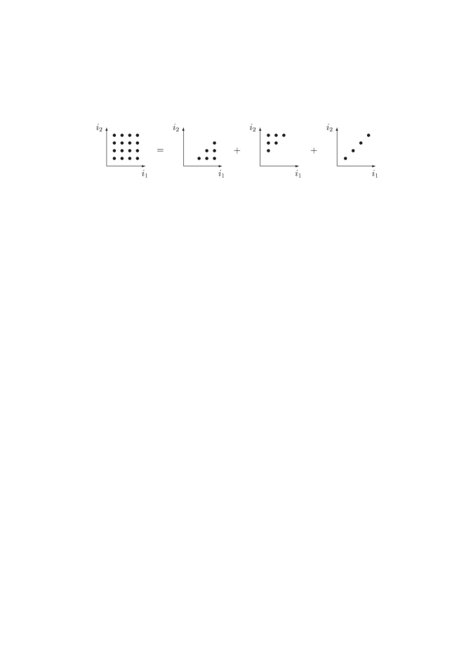
Figure 2: Sketch of the proof for the multiplication of $Z$-sums. The sum over the square is replaced by the sum over the three regions on the r.h.s.

The proof that $Z$-sums obey the quasi-shuffle algebra is sketched in Fig. 2. The outermost sums of the $Z$-sums on the l.h.s of (31) are split into the three regions indicated in Fig. 2. A simple example for the multiplication of two $Z$-sums is

$$Z(n;m_{1};x_{1})Z(n;m_{1};x_{2})=$$ (32)

$$Z(n;m_{1},m_{2};x_{1},x_{2})+Z(n;m_{2},m_{1};x_{2},x_{1})+Z(n;m_{1}+m_{2};x_{1}x_{2}).$$

The quasi-shuffle algebra ${\cal A}$ is isomorphic to the free polynomial algebra on the Lyndon words. If one introduces a lexicographic ordering on the letters of the alphabet $A$, a Lyndon word is defined by the property

$$W<V$$ (33)

for any subwords $U$ and $V$ such that $W=U,V$. Here $U,V$ means just concatenation of $U$ and $V$.

The $Z$-sums form actuall a Hopf algebra. It is convenient to phrase the coalgebra structure in terms of rooted trees. $Z$-sums can be represented as rooted trees without any sidebranchings. As a concrete example the pictorial representation of a sum of depth three reads:

$$Z(n;m_{1},m_{2},m_{3};x_{1},x_{2},x_{3}) = \sum\limits_{i_{1}=1}^{n}\sum\limits_{i_{2}=1}^{i_{1}-1}\sum\limits_{i_{3}=1}^{i_{2}-1}\frac{x_{1}^{i_{1}}}{{i_{1}}^{m_{1}}}\frac{x_{2}^{i_{2}}}{{i_{2}}^{m_{2}}}\frac{x_{3}^{i_{3}}}{{i_{3}}^{m_{3}}}\;\;=\;\;\begin{picture}(40.0,60.0)(-10.0,30.0)\Vertex(10,50){2} \Vertex(10,30){2} \Vertex(10,10){2} \Line(10,10)(10,50) \Text(6,50)[r]{$x_{1}$} \Text(6,30)[r]{$x_{2}$} \Text(6,10)[r]{$x_{3}$} \end{picture}$$ (34)

The outermost sum corresponds to the root. By convention, the root is always drawn on the top. Trees with sidebranchings are given by nested sums with more than one subsum, for example:

$$\sum\limits_{i=1}^{n}\frac{x_{1}^{i}}{i^{m_{1}}}Z(i-1;m_{2},x_{2})Z(i-1;m_{3};x_{3}) = x_{1} x_{2} x_{3}$$ (35)

Of course, due to the multiplication formula, trees with sidebranchings can always be reduced to trees without any sidebranchings. The coalgebra structure is now formulated in terms of rooted trees. I first introduce some notation how to manipulate rooted trees, following the notation of Kreimer and Connes Kreimer:1998dp ; Connes:1998qv . An elementary cut of a rooted tree is a cut at a single chosen edge. An admissible cut is any assignment of elementary cuts to a rooted tree such that any path from any vertex of the tree to the root has at most one elementary cut. An admissible cut maps a tree $t$ to a monomial in trees $t_{1}\circ...\circ t_{k+1}$. Note that precisely one of these subtrees $t_{j}$ will contain the root of $t$. Denote this distinguished tree by $R^{C}(t)$, and the monomial delivered by the $k$ other factors by $P^{C}(t)$. The counit $\bar{e}$ is given by

$$\bar{e}(e) = 1,$$

$$\bar{e}(t) = 0,\;\;\;t\neq e.$$ (36)

The coproduct $\Delta$ is defined by the equations

$$\Delta(e) = e\otimes e,$$

$$\Delta(t) = e\otimes t+t\otimes e+\sum\limits_{\mbox{\tiny adm. cuts $C$ of $t$}}P^{C}(t)\otimes R^{C}(t),$$

$$\Delta(t_{1}\circ...\circ t_{k}) = \Delta(t_{1})(\circ\otimes\circ)...(\circ\otimes\circ)\Delta(t_{k}).$$ (37)

The antipode ${\cal S}$ is given by

$${\cal S}(e) = e,$$

$${\cal S}(t) = -t-\sum\limits_{\mbox{\tiny adm. cuts $C$ of $t$}}{\cal S}\left(P^{C}(t)\right)\circ R^{C}(t),$$

$${\cal S}(t_{1}\circ...\circ t_{k}) = {\cal S}(t_{1})\circ...\circ{\cal S}(t_{k}).$$ (38)

Since the multiplication in the algebra is commutative the antipode satisfies

$${\cal S}^{2} = \mbox{id}.$$ (39)

Let me give some examples for the coproduct and the antipode for $Z$-sums:

$$\Delta Z(n;m_{1};x_{1}) = e\otimes Z(n;m_{1};x_{1})+Z(n;m_{1};x_{1})\otimes e,$$

$$\Delta Z(n;m_{1},m_{2};x_{1},x_{2}) = e\otimes Z(n;m_{1},m_{2};x_{1},x_{2})+Z(n;m_{1},m_{2};x_{1},x_{2})\otimes e$$ (40)

$$+Z(n;m_{2};x_{2})\otimes Z(n;m_{1};x_{1}),$$

$${\cal S}Z(n;m_{1};x_{1}) = -Z(n;m_{1};x_{1}),$$

$${\cal S}Z(n;m_{1},m_{2};x_{1},x_{2}) = Z(n;m_{2},m_{1};x_{2},x_{1})+Z(n;m_{1}+m_{2};x_{1}x_{2}).$$ (41)

The Hopf algebra of nested sums has additional structures if we allow expressions of the form

$$\frac{x_{0}^{n}}{n^{m_{0}}}Z(n;m_{1},...,m_{k};x_{1},...,x_{k}),$$ (42)

e.g. $Z$-sums multiplied by a letter. Then the following convolution product

$$\sum\limits_{i=1}^{n-1}\;\frac{x^{i}}{i^{m}}Z(i-1;...)\;\frac{y^{n-i}}{(n-i)^{m^{\prime}}}Z(n-i-1;...)$$ (43)

can again be expressed in terms of expressions of the form (42). An example is

$$\sum\limits_{i=1}^{n-1}\;\frac{x^{i}}{i}Z_{1}(i-1)\;\frac{y^{n-i}}{(n-i)}Z_{1}(n-i-1)=$$ (44)

$$\frac{x^{n}}{n}\left[Z\left(n-1;1,1,1;\frac{y}{x},\frac{x}{y},\frac{y}{x}\right)+Z\left(n-1;1,1,1;\frac{y}{x},1,\frac{x}{y}\right)\right.$$

$$\left.+Z\left(n-1;1,1,1;1,\frac{y}{x},1\right)\right]+\left(x\leftrightarrow y\right).$$

In addition there is a conjugation, e.g. sums of the form

$$-\sum\limits_{i=1}^{n}\left(\begin{array}[]{c}n\\ i\\ \end{array}\right)\left(-1\right)^{i}\;\frac{x^{i}}{i^{m}}S(i;...)$$ (47)

can also be reduced to terms of the form (42). Although one can easily convert between the notations for $S$-sums and $Z$-sums, expressions involving a conjugation tend to be shorter when expressed in terms of $S$-sums. The name conjugation stems from the following fact: To any function $f(n)$ of an integer variable $n$ one can define a conjugated function $C\circ f(n)$ as the following sum

$$C\circ f(n) = \sum\limits_{i=1}^{n}\left(\begin{array}[]{c}n\\ i\\ \end{array}\right)(-1)^{i}f(i).$$ (50)

Then conjugation satisfies the following two properties:

$$C\circ 1 = 1,$$

$$C\circ C\circ f(n) = f(n).$$ (51)

An example for a sum involving a conjugation is

$$-\sum\limits_{i=1}^{n}\left(\begin{array}[]{c}n\\ i\\ \end{array}\right)\left(-1\right)^{i}\;\frac{x^{i}}{i}S_{1}(i)=$$ (55)

$$S\left(n;1,1;1-x,\frac{1}{1-x}\right)-S\left(n;1,1;1-x,1\right).$$

Finally there is the combination of conjugation and convolution, e.g. sums of the form

$$-\sum\limits_{i=1}^{n-1}\left(\begin{array}[]{c}n\\ i\\ \end{array}\right)\left(-1\right)^{i}\;\frac{x^{i}}{i^{m}}S(i;...)\;\frac{y^{n-i}}{(n-i)^{m^{\prime}}}S(n-i;...)$$ (58)

can also be reduced to terms of the form (42). An example is given by

$$-\sum\limits_{i=1}^{n-1}\left(\begin{array}[]{c}n\\ i\\ \end{array}\right)\left(-1\right)^{i}\;S(i;1;x)\;S(n-i;1;y)=$$

$$\frac{1}{n}\left\{S(n;1;y)+(1-x)^{n}\left[S\left(n;1;\frac{1}{1-\frac{1}{x}}\right)-S\left(n;1;\frac{1-\frac{y}{x}}{1-\frac{1}{x}}\right)\right]\right\}$$

$$+\frac{(-1)^{n}}{n}\left\{S(n;1;x)+(1-y)^{n}\left[S\left(n;1;\frac{1}{1-\frac{1}{y}}\right)-S\left(n;1;\frac{1-\frac{x}{y}}{1-\frac{1}{y}}\right)\right]\right\}.$$

4 Expansion of hypergeometric functions

In this section I discuss how the algebraic tools introduced in the previous section can be used to solve the problems outlined at the end of Sect. 2. First I give some motivation for the introduction of $Z$-sums: The essential point is that $Z$-sums interpolate between multiple polylogarithms and Euler-Zagier-sums, such that the interpolation is compatible with the algebra structure. On the one hand, we expect multiple polylogarithm to appear in the Laurent expansion of the transcendental functions (8)-(17), a fact which is confirmed a posteriori. Therefore it is important that multiple polylogarithms are contained in the class of $Z$-sums. On the other the expansion parameter $\varepsilon$ occurs in the functions (8)-(17) inside the arguments of Gamma-functions. The basic formula for the expansion of Gamma-functions reads

$$\Gamma(n+\varepsilon)=\Gamma(1+\varepsilon)\Gamma(n)\left[1+\varepsilon Z_{1}(n-1)+\varepsilon^{2}Z_{11}(n-1)\right.$$ (63)

$$\left.+\varepsilon^{3}Z_{111}(n-1)+...+\varepsilon^{n-1}Z_{11...1}(n-1)\right],$$

containing Euler-Zagier sums for finite $n$. As a simple example I discuss the expansion of

$$\sum\limits_{i=0}^{\infty}\frac{\Gamma(i+a_{1}+t_{1}\varepsilon)\Gamma(i+a_{2}+t_{2}\varepsilon)}{\Gamma(i+1)\Gamma(i+a_{3}+t_{3}\varepsilon)}x^{i}$$ (64)

into a Laurent series in $\varepsilon$. Here $a_{1}$, $a_{2}$ and $a_{3}$ are assumed to be integers. Up to prefactors the expression in (64) is a hypergeometric function ${}_{2}F_{1}$. Using $\Gamma(x+1)=x\Gamma(x)$, partial fractioning and an adjustment of the summation index one can transform (64) into terms of the form

$$\sum\limits_{i=1}^{\infty}\frac{\Gamma(i+t_{1}\varepsilon)\Gamma(i+t_{2}\varepsilon)}{\Gamma(i)\Gamma(i+t_{3}\varepsilon)}\frac{x^{i}}{i^{m}},$$ (65)

where $m$ is an integer. Now using (63) one obtains

$$\Gamma(1+\varepsilon)\sum\limits_{i=1}^{\infty}\frac{\left(1+\varepsilon t_{1}Z_{1}(i-1)+...\right)\left(1+\varepsilon t_{2}Z_{1}(i-1)+...\right)}{\left(1+\varepsilon t_{3}Z_{1}(i-1)+...\right)}\frac{x^{i}}{i^{m}}.$$ (66)

Inverting the power series in the denominator and truncating in $\varepsilon$ one obtains in each order in $\varepsilon$ terms of the form

$$\sum\limits_{i=1}^{\infty}\frac{x^{i}}{i^{m}}Z_{m_{1}...m_{k}}(i-1)Z_{m_{1}^{\prime}...m_{l}^{\prime}}(i-1)Z_{m_{1}^{\prime\prime}...m_{n}^{\prime\prime}}(i-1)$$ (67)

Using the quasi-shuffle product for $Z$-sums the three Euler-Zagier sums can be reduced to single Euler-Zagier sums and one finally arrives at terms of the form

$$\sum\limits_{i=1}^{\infty}\frac{x^{i}}{i^{m}}Z_{m_{1}...m_{k}}(i-1),$$ (68)

which are harmonic polylogarithms $H_{m,m_{1},...,m_{k}}(x)$. This completes the algorithm for the expansion in $\varepsilon$ for sums of the form (8). Since the one-loop integral discussed in (5) is a special case of (8), this algorithm also applies to the integral (5). In addition, this algorithm shows that in the expansion of hypergeometric functions ${}_{J+1}F_{J}(a_{1},...,a_{J+1};b_{1},...,b_{J};x)$ around integer values of the parameters $a_{k}$ and $b_{l}$ only harmonic polylogarithms appear in the result.

The algorithm for the expansion of sums of type (8) used the multiplication formula for $Z$-sums to pass from (67) to (68). To expand double sums of type (9) one needs in addition the convolution product (43). To expand sums of type (13) the conjugation (47) is needed. Finally, for sums of type (17) the combination of conjugation and convolution as in (58) is required. More details can be found in Moch:2001zr .

Let me come back to the example of the one-loop Feynman integral discussed in Sect. 2. For $\nu_{1}=\nu_{2}=\nu_{3}=1$ and $m=2$ in (5) one obtains:

$$\int\frac{d^{4-2\varepsilon}k_{1}}{i\pi^{2-\varepsilon}}\frac{1}{(-k_{1}^{2})}\frac{1}{(-k_{2}^{2})}\frac{1}{(-k_{3}^{2})}$$ (69)

$$= \frac{\Gamma(-\varepsilon)\Gamma(1-\varepsilon)\Gamma(1+\varepsilon)}{\Gamma(1-2\varepsilon)}\frac{\left(-p_{123}^{2}\right)^{-1-\varepsilon}}{1-x}\sum\limits_{n=1}^{\infty}\varepsilon^{n-1}H_{\underbrace{1,...,1}_{n}}(1-x).$$

Here, all harmonic polylogarithms can be expressed in terms of Nielsen polylogarithms, which in turn simplify to powers of the standard logarithm:

$$H_{\underbrace{1,...,1}_{n}}(1-x) = S_{0,n}(1-x)=\frac{(-1)^{n}}{n!}\left(\ln x\right)^{n}.$$ (70)

This particular example is very simple and one recovers the well-known all-order result

$$\frac{\Gamma(1-\varepsilon)^{2}\Gamma(1+\varepsilon)}{\Gamma(1-2\varepsilon)}\frac{\left(-p_{123}^{2}\right)^{-1-\varepsilon}}{\varepsilon^{2}}\frac{1-x^{-\varepsilon}}{1-x},$$ (71)

which (for this simple example) can also be obtained by direct integration.

5 Multiple polylogarithms

The multiple polylogarithms are special cases of $Z$-sums. They are obtained from $Z$-sums by taking the outermost sum to infinity:

$$Z(\infty;m_{1},...,m_{k};x_{1},...,x_{k}) = \mbox{Li}_{m_{k},...,m_{1}}(x_{k},...,x_{1}).$$ (72)

The reversed order of the arguments and indices on the r.h.s. follows the notation of Goncharov Goncharov . They have been studied extensively in the literature by physicists Remiddi:1999ew ; Vermaseren:1998uu , Gehrmann:2000zt -Moch:2002hm and mathematicians Borwein ,Hain -Racinet:2002 . Here I summarize the most important properties. Being special cases of $Z$-sums they obey the quasi-shuffle Hopf algebra for $Z$-sums. Multiple polylogarithms have been defined in this article via the sum representation (19). In addition, they admit an integral representation. From this integral representation a second algebra structure arises, which turns out to be a shuffle Hopf algebra. To discuss this second Hopf algebra it is convenient to introduce for $z_{k}\neq 0$ the following functions

$$G(z_{1},...,z_{k};y) = \int\limits_{0}^{y}\frac{dt_{1}}{t_{1}-z_{1}}\int\limits_{0}^{t_{1}}\frac{dt_{2}}{t_{2}-z_{2}}...\int\limits_{0}^{t_{k-1}}\frac{dt_{k}}{t_{k}-z_{k}}.$$ (73)

In this definition one variable is redundant due to the following scaling relation:

$$G(z_{1},...,z_{k};y) = G(xz_{1},...,xz_{k};xy)$$ (74)

If one further defines

$$g(z;y) = \frac{1}{y-z},$$ (75)

then one has

$$\frac{d}{dy}G(z_{1},...,z_{k};y) = g(z_{1};y)G(z_{2},...,z_{k};y)$$ (76)

and

$$G(z_{1},z_{2},...,z_{k};y) = \int\limits_{0}^{y}dt\;g(z_{1};t)G(z_{2},...,z_{k};t).$$ (77)

One can sligthly enlarge the set and define $G(0,...,0;y)$ with $k$ zeros for $z_{1}$ to $z_{k}$ to be

$$G(0,...,0;y) = \frac{1}{k!}\left(\ln y\right)^{k}.$$ (78)

This permits us to allow trailing zeros in the sequence $(z_{1},...,z_{k})$ by defining the function $G$ with trailing zeros via (77) and (78). To relate the multiple polylogarithms to the functions $G$ it is convenient to introduce the following short-hand notation:

$$G_{m_{1},...,m_{k}}(z_{1},...,z_{k};y) = G(\underbrace{0,...,0}_{m_{1}-1},z_{1},...,z_{k-1},\underbrace{0...,0}_{m_{k}-1},z_{k};y)$$ (79)

Here, all $z_{j}$ for $j=1,...,k$ are assumed to be non-zero. One then finds

$$\mbox{Li}_{m_{k},...,m_{1}}(x_{k},...,x_{1}) = (-1)^{k}G_{m_{1},...,m_{k}}\left(\frac{1}{x_{1}},\frac{1}{x_{1}x_{2}},...,\frac{1}{x_{1}...x_{k}};1\right).$$ (80)

The inverse formula reads

$$G_{m_{1},...,m_{k}}(z_{1},...,z_{k};y) = (-1)^{k}\;\mbox{Li}_{m_{k},...,m_{1}}\left(\frac{z_{k-1}}{z_{k}},...,\frac{z_{1}}{z_{2}},\frac{y}{z_{1}}\right).$$ (81)

Eq. (80) together with (79) and (73) defines an integral representation for the multiple polylogarithms. To make this more explicit I first introduce some notation for iterated integrals

$$\int\limits_{0}^{\Lambda}\frac{dt}{t-a_{n}}\circ...\circ\frac{dt}{t-a_{1}} = \int\limits_{0}^{\Lambda}\frac{dt_{n}}{t_{n}-a_{n}}\int\limits_{0}^{t_{n}}\frac{dt_{n-1}}{t_{n-1}-a_{n-1}}\times...\times\int\limits_{0}^{t_{2}}\frac{dt_{1}}{t_{1}-a_{1}}$$ (82)

and the short hand notation:

$$\int\limits_{0}^{\Lambda}\left(\frac{dt}{t}\circ\right)^{m}\frac{dt}{t-a} = \int\limits_{0}^{\Lambda}\underbrace{\frac{dt}{t}\circ...\frac{dt}{t}}_{m\;\mbox{times}}\circ\frac{dt}{t-a}.$$ (83)

The integral representation for $\mbox{Li}_{m_{k},...,m_{1}}(x_{k},...,x_{1})$ reads then

$$\mbox{Li}_{m_{k},...,m_{1}}(x_{k},...,x_{1})=(-1)^{k}\int\limits_{0}^{1}\left(\frac{dt}{t}\circ\right)^{m_{1}-1}\frac{dt}{t-b_{1}}$$ (84)

$$\circ\left(\frac{dt}{t}\circ\right)^{m_{2}-1}\frac{dt}{t-b_{2}}\circ...\circ\left(\frac{dt}{t}\circ\right)^{m_{k}-1}\frac{dt}{t-b_{k}},$$

where the $b_{j}$’s are related to the $x_{j}$’s

$$b_{j} = \frac{1}{x_{1}x_{2}...x_{j}}.$$ (85)

From the iterated integral representation (73) a second algebra structure for the functions $G(z_{1},...,z_{k};y)$ (and through (80) also for the multiple polylogarithms) is obtained as follows: We take the $z_{j}$’s as letters and call a sequence of ordered letters $w=z_{1},...,z_{k}$ a word. Then the function $G(z_{1},...,z_{k};y)$ is uniquely specified by the word $w=z_{1},...,z_{k}$ and the variable $y$. The neutral element $e$ is given by the empty word, equivalent to

$$G(;y) = 1.$$ (86)

A shuffle algebra on the vector space of words is defined by

$$e\circ w = w\circ e=w,$$

$$(z_{1},w_{1})\circ(z_{2},w_{2}) = z_{1},(w_{1}\circ(z_{2},w_{2}))+z_{2},((z_{1},w_{1})\circ w_{2}).$$ (87)

Note that this definition is very similar to the definition of the quasi-shuffle algebra (3), except that the third term in (3) is missing. In fact, a shuffle algebra is a special case of a quasi-shuffle algebra, where the product of two letters is degenerate: $X_{1}\cdot X_{2}=0$ for all letters $X_{1}$ and $X_{2}$ in the notation of Sect. 3. The definition of the shuffle product (5) translates into the following recursive definition of the product of two $G$-functions:

$$G(z_{1},...,z_{k};y)\times G(z_{k+1},...,z_{n};y)=$$ (89)

$$\int\limits_{0}^{y}\frac{dt}{t-z_{1}}G(z_{2},...,z_{k};t)G(z_{k+1},...,z_{n};t)$$

$$+\int\limits_{0}^{y}\frac{dt}{t-z_{k+1}}G(z_{1},...,z_{k};t)G(z_{k+2},...,z_{n};t)$$

For the discussion of the coalgebra part for the functions $G(z_{1},...,z_{k};y)$ we may proceed as in Sect. 3 and associate to any function $G(z_{1},...,z_{k};y)$ a rooted tree without sidebranchings as in the following example:

$$G(z_{1},z_{2},z_{3};y) = z_{1} z_{2} z_{3}$$ (90)

The outermost integration (involving $z_{1}$) corresponds to the root. The formulae for the coproduct (3) and the antipode (3) apply then also to the functions $G(z_{1},...,z_{k};y)$.

A shuffle algebra is simpler than a quasi-shuffle algebra and one finds for a shuffle algebra besides the recursive definitions of the product, the coproduct and the antipode also closed formulae for these operations. For the product one has

$$G(z_{1},...,z_{k};y)\;G(z_{k+1},...,z_{k+l};y) = \sum\limits_{shuffle}G\left(z_{\sigma(1)},...,z_{\sigma(k+l)};y\right),$$ (91)

where the sum is over all permutations which preserve the relative order of the strings $z_{1},...,z_{k}$ and $z_{k+1},...,z_{k+l}$. This explains the name “shuffle product”. For the coproduct one has

$$\Delta G(z_{1},...,z_{k};y) = \sum\limits_{j=0}^{k}G(z_{1},...,z_{j};y)\otimes G(z_{j+1},...,z_{k};y)$$ (92)

and for the antipode one finds

$${\cal S}G(z_{1},...,z_{k};y) = (-1)^{k}G(z_{k},...,z_{1};y).$$ (93)

The shuffle multiplication is commutative and the antipode satisfies therefore

$${\cal S}^{2} = \mbox{id}.$$ (94)

From (93) this is evident.

6 The antipode and integration-by-parts

Integration-by-parts has always been a powerful tool for calculations in particle physics. By using integration-by-parts one may obtain an identity between various $G$-functions. The starting point is as follows:

$$G(z_{1},...,z_{k};y)=\int\limits_{0}^{y}dt\left(\frac{\partial}{\partial t}G(z_{1};t)\right)G(z_{2},...,z_{k};y)$$ (95)

$$=G(z_{1};y)G(z_{2},...,z_{k};y)-\int\limits_{0}^{y}dt\;G(z_{1};t)g(z_{2};t)G(z_{3},...,z_{k};y)$$

$$=G(z_{1};y)G(z_{2},...,z_{k};y)-\int\limits_{0}^{y}dt\left(\frac{\partial}{\partial t}G(z_{2},z_{1};t)\right)G(z_{3},...,z_{k};y).$$

Repeating this procedure one arrives at the following integration-by-parts identity:

$$G(z_{1},...,z_{k};y)+(-1)^{k}G(z_{k},...,z_{1};y)$$ (96)

$$= G(z_{1};y)G(z_{2},...,z_{k};y)-G(z_{2},z_{1};y)G(z_{3},...,z_{k};y)+...$$

$$-(-1)^{k-1}G(z_{k-1},...z_{1};y)G(z_{k};y),$$

which relates the combination $G(z_{1},...,z_{k};y)+(-1)^{k}G(z_{k},...,z_{1};y)$ to $G$-functions of lower depth. This relation is useful in simplifying expressions. Eq. (96) can also be derived in a different way. In a Hopf algebra we have for any non-trivial element $w$ the following relation involving the antipode:

$$\sum\limits_{(w)}w^{(1)}\cdot{\cal S}(w^{(2)}) = 0.$$ (97)

Here Sweedler’s notation has been used. Sweedler’s notation writes the coproduct of an element $w$ as

$$\Delta(w) = \sum\limits_{(w)}w^{(1)}\otimes w^{(2)}.$$ (98)

Working out the relation (97) for the shuffle algebra of the functions $G(z_{1},...,$ $z_{k};y)$, we recover (96).

We may now proceed and check if (97) provides also a non-trivial relation for the quasi-shuffle algebra of $Z$-sums. This requires first some notation: A composition of a positive integer $k$ is a sequence $I=(i_{1},...,i_{l})$ of positive integers such that $i_{1}+...i_{l}=k$. The set of all composition of $k$ is denoted by ${\cal C}(k)$. Compositions act on $Z$-sums as

$$(i_{1},...,i_{l})\circ Z(n;m_{1},...,m_{k};x_{1},...,x_{k})$$ (99)

$$= Z\left(n;m_{1}+...+m_{i_{1}},m_{i_{1}+1}+...+m_{i_{1}+i_{2}},...,m_{i_{1}+...+i_{l-1}+1}+...\right.$$

$$\left.+m_{i_{1}+...+i_{l}};x_{1}...x_{i_{1}},x_{i_{1}+1}...x_{i_{1}+i_{2}},...,x_{i_{1}+...+i_{l-1}+1}...x_{i_{1}+...+i_{l}}\right),$$

e.g. the first $i_{1}$ letters of the $Z$-sum are combined into one new letter, the next $i_{2}$ letters are combined into the second new letter, etc.. With this notation for compositions one obtains the following closed formula for the antipode in the quasi-shuffle algebra:

$${\cal S}Z(n;m_{1},...,m_{k};x_{1},...,x_{k}) = (-1)^{k}\sum\limits_{I\in{\cal C}(k)}I\circ Z(n;m_{k},...,m_{1};x_{k},...,x_{1})$$

From (97) we then obtain

$$Z(n;m_{1},...,m_{k};x_{1},...,x_{k})+(-1)^{k}Z(n;m_{k},...,m_{1};x_{k},...,x_{1})$$ (101)

$$= -\sum\limits_{adm.\;cuts}P^{C}(Z(n;m_{1},...,m_{k};x_{1},...,x_{k}))$$

$$\cdot{\cal S}\left(R^{C}(Z(n;m_{1},...,m_{k};x_{1},...,x_{k}))\right)$$

$$-(-1)^{k}\sum\limits_{I\in{\cal C}(k)\backslash(1,1,...,1)}I\circ Z(n;m_{k},...,m_{1};x_{k},...,x_{1}).$$

Again, the combination $Z(n;m_{1},...,m_{k};x_{1},...,x_{k})+(-1)^{k}Z(n;m_{k},...,m_{1};x_{k},$ $...,x_{1})$ reduces to $Z$-sums of lower depth, similar to (96). We therefore obtained an “integration-by-parts” identity for objects, which don’t have an integral representation. We first observed, that for the $G$-functions, which have an integral representation, the integration-by-parts identites are equal to the identities obtained from the antipode. After this abstraction towards an algebraic formulation, one can translate these relations to cases, which only have the appropriate algebra structure, but not necessarily a concrete integral representation. As an example we have

$$Z(n;m_{1},m_{2},m_{3};x_{1},x_{2},x_{3})-Z(n;m_{3},m_{2},m_{1};x_{3},x_{2},x_{1})=$$ (102)

$$Z(n;m_{1};x_{1})Z(n;m_{2},m_{3};x_{2},x_{3})-Z(n;m_{2},m_{1};x_{2},x_{1})Z(n;m_{3};x_{3})$$

$$-Z(n;m_{1}+m_{2};x_{1}x_{2})Z(n;m_{3};x_{3})+Z(n;m_{2}+m_{3},m_{1};x_{2}x_{3},x_{1})$$

$$+Z(n;m_{3},m_{1}+m_{2};x_{3},x_{1}x_{2})+Z(n;m_{1}+m_{2}+m_{3};x_{1}x_{2}x_{3}),$$

which expresses the combination of the two $Z$-sums of depth $3$ as $Z$-sums of lower depth. The analog example for the shuffle algebra of the $G$-function reads:

$$G(z_{1},z_{2},z_{3};y)-G(z_{3},z_{2},z_{1};y) = G(z_{1};y)G(z_{2},z_{3};y)-G(z_{2},z_{1};y)G(z_{3};y).$$

Multiple polylogarithms obey both the quasi-shuffle algebra and the shuffle algebra. Therefore we have for multiple polylogarithms two relations, which are in general independent.

7 Summary

In this article I discussed the mathematics underlying the calculation of Feynman loop integrals. The algorithms are based on $Z$-sums, which form a Hopf algebra with a quasi-shuffle product. This algebra has as additional structure a conjugation and a convolution product. In the final results multiple polylogarithms appear. Multiple polylogarithms obey apart from the quasi-shuffle algebra a second Hopf algebra. This additional Hopf algebra has a shuffle product.

8 Notations and conventions

There are several notations for the multiple polylogarithms. I briefly summmarize them here. In this article multiple polylogarithms are defined via the sum representation

$$\mbox{Li}_{m_{k},...,m_{1}}(x_{k},...,x_{1}) = Z(\infty;m_{1},...,m_{k};x_{1},...,x_{k}).$$ (104)

The reversed order of the arguments and indices for $\mbox{Li}_{m_{k},...,m_{1}}(x_{k},...,x_{1})$ follows the notation of Goncharov Goncharov . Gehrmann and Remiddi Gehrmann:2001pz ; Gehrmann:2001jv ; Gehrmann:2002zr use the notation $G(z_{1},...,z_{k};y)$ and $G_{m_{1},...,m_{k}}(z_{1}^{\prime},...,z_{k}^{\prime};y)$. The relation with the notation above is

$$\mbox{Li}_{m_{k},...,m_{1}}(x_{k},...,x_{1}) = (-1)^{k}G_{m_{1},...,m_{k}}\left(b_{1},b_{2},...,b_{k};1\right),$$ (105)

where

$$b_{j} = \frac{1}{x_{1}x_{2}...x_{j}}.$$ (106)

Borwein, Bradley, Broadhurst and Lisonek Borwein denote multiple polylogarithms as

$$\lambda\left(\begin{array}[]{c}m_{1},...,m_{k}\\ b_{1},...,b_{k}\\ \end{array}\right) = \mbox{Li}_{m_{k},...,m_{1}}(x_{k},...,x_{1})$$ (109)

In the french literature Minh:2000 ; Cartier:2001 harmonic polylogarithms are often denoted as

$$\mbox{Li}_{m_{1},...,m_{k}}(x) = H_{m_{1},...,m_{k}}(x)$$ (110)

and referred to as “multiple polylogarithms of a single variable”. Note the order of the indices for $\mbox{Li}_{m_{1},...,m_{k}}(x)$ in (110).

References

- (1) O. V. Tarasov, Phys. Rev. D54, 6479 (1996), hep-th/9606018.
- (2) O. V. Tarasov, Nucl. Phys. B502, 455 (1997), hep-ph/9703319.
- (3) J. A. M. Vermaseren, math-ph/0010025.
- (4) C. Bauer, A. Frink, and R. Kreckel, J. Symbolic Computation 33, 1 (2002), cs.sc/0004015.
- (5) S. Weinzierl, Comput. Phys. Commun. 145, 357 (2002), math-ph/0201011.
- (6) S. Moch, P. Uwer, and S. Weinzierl, J. Math. Phys. 43, 3363 (2002), hep-ph/0110083.
- (7) L. Euler, Novi Comm. Acad. Sci. Petropol. 20, 140 (1775).
- (8) D. Zagier, First European Congress of Mathematics, Vol. II, Birkhauser, Boston, 497 (1994).
- (9) J. M. Borwein, D. M. Bradley, D. J. Broadhurst and P. Lisonek, Trans. Amer. Math. Soc. 353:3, 907 (2001), math.CA/9910045.
- (10) L. Lewin, ”Polylogarithms and associated functions”, (North Holland, Amsterdam, 1981).
- (11) N. Nielsen, Nova Acta Leopoldina (Halle) 90, 123 (1909).
- (12) E. Remiddi and J. A. M. Vermaseren, Int. J. Mod. Phys. A15, 725 (2000), hep-ph/9905237.
- (13) J. A. M. Vermaseren, Int. J. Mod. Phys. A14, 2037 (1999), hep-ph/9806280.
- (14) M. E. Hoffman, J. Algebraic Combin. 11, 49 (2000), math.QA/9907173.
- (15) D. Kreimer, Adv. Theor. Math. Phys. 2, 303 (1998), q-alg/9707029.
- (16) A. Connes and D. Kreimer, Commun. Math. Phys. 199, 203 (1998), hep-th/9808042.
- (17) T. Gehrmann and E. Remiddi, Nucl. Phys. B601, 248 (2001), hep-ph/0008287.
- (18) T. Gehrmann and E. Remiddi, Comput. Phys. Commun. 141, 296 (2001), hep-ph/0107173.
- (19) T. Gehrmann and E. Remiddi, Comput. Phys. Commun. 144, 200 (2002), hep-ph/0111255.
- (20) T. Gehrmann and E. Remiddi, Nucl. Phys. B640, 379 (2002), hep-ph/0207020.
- (21) S. Moch, P. Uwer, and S. Weinzierl, Phys. Rev. D66, 114001 (2002), hep-ph/0207043.
- (22) R. M. Hain, alg-geom/9202022.
- (23) A. B. Goncharov, Math. Res. Lett. 5, 497 (1998).
- (24) A. B. Goncharov, math.AG/0103059.
- (25) A. B. Goncharov, math.AG/0207036.
- (26) A. B. Goncharov, math.AG/0208144.
- (27) P. Elbaz-Vincent and H. Gangl, Comp. Math. 130, 161 (2002), math.KT/0008089.
- (28) H. Gangl, math.KT/0207222.
- (29) H. M. Minh, M. Petitot and J. van der Hoeven, Discrete Math. 225:1-3, 217 (2000).
- (30) P. Cartier, Séminaire Bourbaki , 885 (2001), in french.
- (31) J. Ecalle, Preprint Orsay 2002-23, (2002), in french with additional grammatical inventions, http://www.math.u-psud.fr/~biblio/ppo/2002/ppo2002-23.html.
- (32) G. Racinet, math.QA/0202142, in french.