On the Dirichlet Boundary Problem and Hirota Equations

We review the integrable structure of the Dirichlet boundary problem in two dimensions. The solution to the Dirichlet boundary problem for simply-connected case is given through a quasiclassical tau-function, which satisfies the Hirota equations of the dispersionless Toda hierarchy, following from properties of the Dirichlet Green function. We also outline a possible generalization to the case of multiply-connected domains related to the multi-support solutions of matrix models.

1 Introduction: the Green function and the Hadamard formula

Solving the Dirichlet boundary problem [1], one reconstructs a harmonic function in a bounded domain from its values on the boundary. In two dimensions, this is one of standard problems of complex analysis having close relations to string theory and matrix models. Remarkably, it possesses a hidden integrable structure [2]. It turns out that variation of a solution to the Dirichlet problem under variation of the domain is described by an infinite hierarchy of non-linear partial differential equations known (in the simply-connected case) as dispersionless Toda hierarchy. It is a particular example of the universal hierarchy of quasiclassical or Whitham equations introduced in [3, 4].

The quasiclassical tau-function (or its logarithm $F$) is the main new object associated with a family of domains in the plane. Any domain in the complex plane with sufficiently smooth boundary can be parametrized by its harmonic moments and the $F$-function is a function of the full infinite set of the moments. The first order derivatives of $F$ are then moments of the complementary domain. This gives a formal solution to the inverse potential problem, considered for a simply-connected case in [5, 6]. The second order derivatives are coefficients of the Taylor expansion of the Dirichlet Green function and therefore they solve the Dirichlet boundary problem. These coefficients are constrained by infinite number of universal (i.e. domain-independent) relations which, unified in a generating form, just constitute the dispersionless Hirota equations. For the third order derivatives there is a nice “residue formula” which allows one to prove [7] that $F$ obeys the Witten-Dijkgraaf-Verlinde-Verlinde (WDVV) equaitons [8].

Let us remind the formulation of the Dirichlet problem in planar domains. Let ${\sf D^{c}}$ be a domain in the complex plane bounded by one or several non-intersecting curves. It will be convenient for us to realize the ${\sf D^{c}}$ as a complement of another domain, ${\sf D}$ (which in general may have more than one connected components), and consider the Dirichlet problem in ${\sf D^{c}}$. The problem is to find a harmonic function $u(z)$ in ${\sf D^{c}}$, such that it is continuous up to the boundary $\partial{\sf D^{c}}$ and equals a given function $u_{0}(\xi)$ on the boundary, and it can be uniquely solved in terms of the Dirichlet Green function $G(z,\xi)$:

$$\begin{array}[]{c}u(z)=-\frac{1}{2\pi}\oint_{\partial{\sf D^{c}}}u_{0}(\xi)\partial_{n}G(z,\xi)|d\xi|\end{array}$$ (1.1)

where $\partial_{n}$ is the normal derivative on the boundary with respect to the second variable, and the normal vector $\vec{n}$ is directed inward ${\sf D^{c}}$, $|d\xi|:=dl(\xi)$ is an infinitesimal element of the length of the boundary $\partial{\sf D^{c}}$.

The Dirichlet Green function is uniquely determined by the following properties [1]:

• The function $G(z,z^{\prime})$ is symmetric and harmonic everywhere in ${\sf D^{c}}$ (including $\infty$ if ${\sf D^{c}}\ni\infty$) in both arguments except $z=z^{\prime}$ where $G(z,z^{\prime})=\log|z-z^{\prime}|+\ldots$ as $z\to z^{\prime}$;

• $G(z,z^{\prime})=0$ if any of the variables $z$, $z^{\prime}$ belongs to the boundary.

Note that the definition implies that $G(z,z^{\prime})<0$ inside ${\sf D^{c}}$. In particular, $\partial_{n}G(z,\xi)$ is strictly negative for all $\xi\in\partial{\sf D^{c}}$.

If ${\sf D^{c}}$ is simply-connected (the boundary has only one component), the Dirichlet problem is equivalent to finding a bijective conformal map from ${\sf D^{c}}$ onto the unit disk or any other reference domain (where the Green function is known explicitly) which exists by virtue of the Riemann mapping theorem. Let $w(z)$ be such a bijective conformal map of ${\sf D^{c}}$ onto the complement to the unit disk, then

$$\begin{array}[]{c}G(z,z^{\prime})=\log\left|\frac{w(z)-w(z^{\prime})}{w(z)\overline{w(z^{\prime})}-1}\right|\end{array}$$ (1.2)

where bar means complex conjugation. It is this formula which allows one to derive the Hirota equations for the tau-function of the Dirichlet problem in the most economic and transparent way [2]. Indeed, the Green function is shown to admit a representation through the logarithm of the tau-function of the form

$$\begin{array}[]{c}G(z,z^{\prime})=\log\left|\frac{1}{z}-\frac{1}{z^{\prime}}\right|+\frac{1}{2}\nabla(z)\nabla(z^{\prime})F\end{array}$$ (1.3)

where $\nabla(z)$ (see (2.5) below) is certain differential operator with constant coefficients (depending only on the point $z$ as a parameter) in the space of harmonic moments. Taking into account that $G(z,\infty)=-\log|w(z)|$, one excludes the Green function from these relations thus obtaining a closed system of equations for $F$ only.

Figure 1: A “pictorial” derivation of the Hadamard formula. We consider a small deformation of the domain, with the new boundary being depicted by the dashed line. According to ($G2$) the Dirichlet Green function vanishes $G(z,\xi)=0$ if $\xi$ belongs to the old boundary. Then the variation $\delta G(z,\xi)$ simply equals to the new value, i.e. in the leading order $\delta G(z,\xi)=-\delta n(\xi)\partial_{n}G(z,\xi)$. Now notice that $\delta G(z,\xi)$ is a harmonic function (the logarithmic singularity cancels since it is the same for both old and new functions) with the boundary value $-\delta n(\xi)\partial_{n}G(z,\xi)$. Applying (1.1) one obtains (1.4).

Our main tool to derive (1.3) is the Hadamard variational formula [9] which gives variation of the Dirichlet Green function under small deformations of the domain in terms of the Green function itself:

$$\begin{array}[]{c}\delta G(z,z^{\prime})=\frac{1}{2\pi}\oint_{\partial{\sf D^{c}}}\partial_{n}G(z,\xi)\partial_{n}G(z^{\prime},\xi)\delta n(\xi)|d\xi|.\end{array}$$ (1.4)

Here $\delta n(\xi)$ is the normal displaycement (with sign) of the boundary under the deformation, counted along the normal vector at the boundary point $\xi$. It was shown in [2] that this remarkable formula reflects all integrable properties of the Dirichlet problem. An extremely simple “pictorial” derivation of the Hadamard formula is presented in fig. 1. Looking at the figure and applying (1.1), one immediately gets (1.4).

2 The Dirichlet problem for simply-connected domains and dispersionless Hirota equations

Let ${\sf D}$ be a connected domain in the complex plane bounded by a simple analytic curve. We consider the exterior Dirichlet problem in ${\sf D^{c}}={\bf C}\setminus{\sf D}$ which is the complement of ${\sf D}$ in the whole (extended) complex plane. Without loss of generality, we assume that ${\sf D}$ is compact and contains the point $z=0$. Then ${\sf D^{c}}$ is an unbounded simply-connected domain containing $\infty$.

2.1 Harmonic moments and elementary deformations

To characterize the shape of the domain ${\sf D^{c}}$ we consider its moments with respect to a complete basis of harmonic functions. The simplest basis is $\{z^{-k}\}$, $\{\bar{z}^{-k}\}$ ($k\geq 1$) and the constant function. Let $t_{k}$ be the harmonic moments

$$\begin{array}[]{c}t_{k}=\,-\,\frac{1}{\pi k}\int_{{\sf D^{c}}}z^{-k}\,d^{2}z\,,\,\;\;\;\;\;k=1,2,\ldots\end{array}$$ (2.1)

and ${\bar{t}}_{k}$ be the complex conjugated moments. The Stokes formula represents them as contour integrals $t_{k}=\frac{1}{2\pi ik}\oint_{\partial{\sf D}}z^{-k}\bar{z}dz$, providing, in particular, a regularization of possibly divergent integrals (2.1). The moment of constant function is infinite but its variation is always finite and opposite to the variation of the complimentary domain ${\sf D}$. Let $t_{0}$ be the area (divided by $\pi$) of ${\sf D}$:

$$\begin{array}[]{c}t_{0}=\frac{1}{\pi}\int_{{\sf D}}d^{2}z\end{array}$$ (2.2)

The harmonic moments of ${\sf D^{c}}$ are coefficients of the Taylor expansion of the potential

$$\begin{array}[]{c}\Phi(z)=-\frac{2}{\pi}\int_{{\sf D}}\log|z-z^{\prime}|d^{2}z^{\prime}\end{array}$$ (2.3)

induced by the domain ${\sf D}$ filled by two-dimensional Coulomb charges with the uniform density $-1$. Clearly, $\partial_{z}\partial_{\bar{z}}\Phi(z)=-1$ if $z\in{\sf D}$ and vanishes otherwise, so around the origin (recall that ${\sf D}\ni 0$) the potential is $-|z|^{2}$ plus a harmonic function:

$$\Phi(z)-\Phi(0)=-|z|^{2}+\sum_{k\geq 1}\left(t_{k}z^{k}+\bar{t}_{k}\bar{z}^{k}\right)$$ (2.4)

A simple calculation shows that $t_{k}$ are just given by (2.1).

The basic fact of the theory of deformations of closed analytic curves is that the (in general complex) moments $\{t_{k},\bar{t}_{k}\}\equiv\{t_{\pm k}\}$ supplemented by the real variable $t_{0}$ form a set of local coordinates in the “moduli space” of smooth closed curves. This means that under any small deformation of the domain the set ${\bf t}=\{t_{0},t_{\pm k}\}$ is subject to a small change and vice versa. For more details, see [10, 11, 12]. The differential operators

$$\begin{array}[]{c}\nabla(z)=\partial_{t_{0}}+\sum_{k\geq 1}\left(\frac{z^{-k}}{k}\partial_{t_{k}}+\frac{\bar{z}^{-k}}{k}\partial_{\bar{t}_{k}}\right)\end{array}$$ (2.5)

span the complexified tangent space to the space of curves. The operator $\nabla(z)$ has a clear geometrical meaning. To clarify it, we introduce the notion of elementary deformation.

Fix a point $z\in{\sf D^{c}}$ and consider a special infinitesimal deformation of the domain such that the normal displaycement of the boundary is proportional to the gradient of the Green function at the boundary point (fig. 2):

$$\delta n(\xi)=-\frac{\epsilon}{2}\partial_{n}G(z,\xi)$$ (2.6)

For any sufficiently smooth initial boundary this deformation is well-defined as $\epsilon\to 0$. We call infinitesimal deformations from this family, parametrized by $z\in{\sf D^{c}}$, elementary deformations. The point $z$ is refered to as the base point of the deformation. Note that since $\partial_{n}G<0$ (see the remark after the definition of the Green function in the Introduction), $\delta n$ for the elementary deformations is either strictly positive or strictly negative depending of the sign of the $\epsilon$.

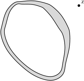
Figure 2: The elementary deformation with the base point $z$.

Let $\delta_{z}$ be variation of any quantity under the elementary deformation with the base point $z$. It is easy to see that $\delta_{z}t_{0}=\epsilon$, $\delta_{z}t_{k}=\epsilon z^{-k}/k$. Indeed,

$$\begin{array}[]{c}\delta_{z}t_{k}=\frac{1}{\pi k}\oint\xi^{-k}\delta n(\xi)|d\xi|=-\frac{\epsilon}{2\pi k}\oint\xi^{-k}\partial_{n}G(z,\xi)|d\xi|={\epsilon\over k}\ z^{-k}\end{array}$$ (2.7)

by virtue of the Dirichlet formula (1.1).

Let $X=X({\bf t})$ be any functional of our domain that depends on the harmonic moments only (in what follows we are going to consider only such functionals). The variation $\delta_{z}X$ in the leading order in $\epsilon$ is then given by

$$\begin{array}[]{c}\delta_{z}X=\sum_{k}\frac{\partial X}{\partial t_{k}}\,\delta_{z}t_{k}=\epsilon\nabla(z)X\end{array}$$ (2.8)

The right hand side suggests that for functionals $X$ such that the series $\nabla(z)X$ converges everywhere in ${\sf D^{c}}$ up to the boundary, $\delta_{z}X$ is a harmonic function of the base point $z$.

Note that in [2] we used the “bump” deformation and continued it harmonically to ${\sf D^{c}}$. So it was the elementary deformation (2.7) $\delta_{z}\propto\oint|d\xi|\partial_{n}G(z,\xi)\delta^{\rm bump}(\xi)$ that was really used. The “bump” deformation should be understood as a (carefully taken) limit of $\delta_{z}$ when the point $z$ tends to the boundary.

2.2 The Hadamard formula as integrability condition

Variation of the Green function under small deformations of the domain is known due to Hadamard, see eq. (1.4). To find how the Green function changes under small variations of the harmonic moments, we fix three points $a,b,c\in{\bf C}\setminus{\sf D}$ and compute $\delta_{c}G(a,b)$ by means of the Hadamard formula (1.4). Using (2.8), one can identify the result with the action of the vector field $\nabla(c)$ on the Green function:

$$\begin{array}[]{c}\nabla(c)G(a,b)=-\,\frac{1}{4\pi}\oint_{\partial{\sf D}}\partial_{n}G(a,\xi)\partial_{n}G(b,\xi)\partial_{n}G(c,\xi)|d\xi|\end{array}$$ (2.9)

Remarkably, the r.h.s. of (2.9) is symmetric in all three arguments:

$$\begin{array}[]{c}\nabla(a)G(b,c)=\nabla(b)G(c,a)=\nabla(c)G(a,b)\end{array}$$ (2.10)

This is the key relation, which allows one to represent the Dirichlet problem as an integrable hierarchy of non-linear differential equations [2]. This relation is the integrability condition of the hierarchy.

It follows from (2.10) (see [2] for details) that there exists a function $F=F({\bf t})$ such that

$$\begin{array}[]{c}G(z,z^{\prime})=\log\left|{1\over z}-{1\over z^{\prime}}\right|+{1\over 2}\nabla(z)\nabla(z^{\prime})F\end{array}$$ (2.11)

The function $F$ is (logarithm of) the tau-function of the integrable hierarchy. In [13] it was called the tau-function of the (real analytic) curves. Existence of such a representation of the Green function was first conjectured by Takhtajan. This formula was first obtained in [13] (see also [12] for a detailed proof and discussion).

2.3 Dispersionless Hirota equations for $F$

Combining (2.11) and (1.2), we obtain the relation

$$\log\left|\frac{w(z)-w(z^{\prime})}{w(z)\overline{w(z^{\prime})}-1}\right|^{2}=\log\left|{1\over z}-{1\over z^{\prime}}\right|^{2}+\nabla(z)\nabla(z^{\prime})F$$ (2.12)

which implies an infinite hierarchy of differential equations on the function $F$. It is convenient to normalize the conformal map $w(z)$ by the conditions that $w(\infty)=\infty$ and $\partial_{z}w(\infty)$ is real, so that

$$w(z)=\frac{z}{r}+O(1)\;\;\;\mbox{as $z\to\infty$}$$ (2.13)

where the real number $r=\lim_{z\to\infty}{dz/dw(z)}$ is called the (external) conformal radius of the domain ${\sf D}$ (equivalently, it can be defined through the Green function as $\log r=\lim_{z\to\infty}(G(z,\infty)+\log|z|)$, see [14]). Then, tending $z^{\prime}\to\infty$ in (2.12), one gets

$$\begin{array}[]{c}\log|w(z)|^{2}=\log|z|^{2}-\partial_{t_{0}}\nabla(z)F\end{array}$$ (2.14)

The limit $z\to\infty$ of this equality yields a simple formula for the conformal radius:

$$\begin{array}[]{c}\log r^{2}=\partial_{t_{0}}^{2}F\end{array}$$ (2.15)

Let us now separate holomorphic and antiholomorphic parts of these equations. To do that it is convenient to introduce holomorphic and antiholomorphic parts of the operator $\nabla(z)$ (2.5):

$$D(z)=\sum_{k\geq 1}\frac{z^{-k}}{k}\partial_{t_{k}}\,,\;\;\;\;\;\bar{D}(\bar{z})=\sum_{k\geq 1}\frac{\bar{z}^{-k}}{k}\partial_{\bar{t}_{k}}\,,$$ (2.16)

Rewrite (2.12) in the form

$$\begin{array}[]{ll}&\displaystyle{\log\left(\frac{w(z)-w(z^{\prime})}{w(z)\overline{w(z^{\prime})}-1}\right)-\log\left(\frac{1}{z}-\frac{1}{z^{\prime}}\right)-\left(\frac{1}{2}\partial_{t_{0}}+D(z)\right)\nabla(z^{\prime})F}\,=\\ &\\ =&\displaystyle{-\log\left(\frac{\overline{w(z)}-\overline{w(z^{\prime})}}{w(z^{\prime})\overline{w(z)}-1}\right)+\log\left(\frac{1}{\bar{z}}-\frac{1}{\bar{z}^{\prime}}\right)+\left(\frac{1}{2}\partial_{t_{0}}+\bar{D}(\bar{z})\right)\nabla(z^{\prime})F}\end{array}$$

The l.h.s. is a holomorphic function of $z$ while the r.h.s. is antiholomorphic. Therefore, both are equal to a $z$-independent term which can be found from the limit $z\to\infty$. As a result, we obtain the equation

$$\begin{array}[]{c}\log\left(\frac{w(z)-w(z^{\prime})}{w(z)-(\overline{w(z^{\prime})})^{-1}}\right)=\log\left(1-\frac{z^{\prime}}{z}\right)+D(z)\nabla(z^{\prime})F\end{array}$$ (2.17)

which, as $z^{\prime}\to\infty$, turns into the formula for the conformal map $w(z)$:

$$\begin{array}[]{c}\log w(z)=\log z-\frac{1}{2}\partial^{2}_{t_{0}}F-\partial_{t_{0}}D(z)F\end{array}$$ (2.18)

(here we used (2.15)). Proceeding in a similar way, one can rearrange (2.17) in order to write it separately for holomorphic and antiholomorphic parts in $z^{\prime}$:

$$\begin{array}[]{c}\log\frac{w(z)-w(z^{\prime})}{z-z^{\prime}}\,=\,-\,\frac{1}{2}\partial_{t_{0}}^{2}\,F+D(z)D(z^{\prime})F\end{array}$$ (2.19)

$$\begin{array}[]{c}-\,\log\left(1-\frac{1}{w(z)\overline{w(z^{\prime})}}\right)=D(z)\bar{D}(\bar{z}^{\prime})F\end{array}$$ (2.20)

Writing down eqs. (2.19) for the pairs of points $(a,b)$, $(b,c)$ and $(c,a)$ and summing up the exponentials of the both sides of each equation one arrives at the relation

$$\begin{array}[]{c}(a-b)e^{D(a)D(b)F}+(b-c)e^{D(b)D(c)F}+(c-a)e^{D(c)D(a)F}=0\end{array}$$ (2.21)

which is the dispersionless Hirota equation (for the KP part of the two-dimensional Toda lattice hierarchy) written in the symmetric form. This equation can be regarded as a very degenerate case of the trisecant Fay identity. It encodes the algebraic relations between the second order derivatives of the function $F$. As $c\to\infty$, we get these relations in a more explicit but less symmetric form:

$$\begin{array}[]{c}1-e^{D(a)D(b)F}=\frac{D(a)-D(b)}{a-b}\,\partial_{t_{1}}F\end{array}$$ (2.22)

which makes it clear that the totality of second derivatives $F_{ij}:=\partial_{t_{i}}\partial_{t_{j}}F$ are expressed through the derivatives with one of the indices equal to unity.

More general equations of the dispersionless Toda hierarchy obtained in a similar way by combining eqs. (2.18), (2.19) and (2.20) include derivatives w.r.t. $t_{0}$ and $\bar{t}_{k}$:

$$\begin{array}[]{c}(a-b)e^{D(a)D(b)F}=ae^{-\partial_{t_{0}}D(a)F}-be^{-\partial_{t_{0}}D(b)F}\end{array}$$ (2.23)

$$\begin{array}[]{c}1-e^{-D(z)\bar{D}(\bar{z})F}=\frac{1}{z\bar{z}}e^{\partial_{t_{0}}\nabla(z)F}\end{array}$$ (2.24)

These equations allow one to express the second derivatives $\partial_{t_{m}}\partial_{t_{n}}F$, $\partial_{t_{m}}\partial_{\bar{t}_{n}}F$ with $m,n\geq 1$ through the derivatives $\partial_{t_{0}}\partial_{t_{k}}F$, $\partial_{t_{0}}\partial_{\bar{t}_{k}}F$. In particular, the dispersionless Toda equation,

$$\begin{array}[]{c}\partial_{t_{1}}\partial_{\bar{t}_{1}}F=e^{\partial_{t_{0}}^{2}F}\end{array}$$ (2.25)

which follows from (2.24) as $z\to\infty$, expresses $\partial_{t_{1}}\partial_{\bar{t}_{1}}F$ through $\partial_{t_{0}}^{2}F$.

For a comprehensive exposition of Hirota equations for dispersionless KP and Toda hierarchies we refer the reader to [15, 16].

2.4 Integral representation of the tau-function

Eq. (2.11) allows one to obtain a representation of the tau-function as a double integral over the domain ${\sf D}$. Set $\tilde{\Phi}(z):=\nabla(z)F$. One is able to determine this function via its variation under the elementary deformation:

$$\delta_{a}\tilde{\Phi}(z)=-2\epsilon\log\left|a^{-1}-z^{-1}\right|+2\epsilon G(a,z)$$ (2.26)

which is read from eq. (2.11) by virtue of (2.8). This allows one to identify $\tilde{\Phi}$ with the “modified potential” $\tilde{\Phi}(z)=\Phi(z)-\Phi(0)+t_{0}\log|z|^{2}$, where $\Phi$ is given by (2.3). Thus we can write

$$\begin{array}[]{c}\nabla(z)F=\tilde{\Phi}(z)=-\frac{2}{\pi}\int_{{\sf D}}\log|z^{-1}-\zeta^{-1}|d^{2}\zeta=v_{0}+2{\rm Re}\sum_{k>0}\frac{v_{k}}{k}z^{-k}\end{array}$$ (2.27)

The last equality is to be understood as the Taylor expansion around infinity. The coefficients $v_{k}$ are moments of the interior domain (the “dual” harmonic moments) defined as

$$\begin{array}[]{c}v_{k}=\frac{1}{\pi}\int_{{\sf D}}z^{k}\,d^{2}z\ \ \ (k>0)\,,\;\;\;\;\;v_{0}=-\Phi(0)=\frac{2}{\pi}\int_{{\sf D}}\log|z|d^{2}z\end{array}$$ (2.28)

From (2.27) it is clear that

$$\begin{array}[]{c}v_{k}=\partial_{t_{k}}F\,,\;\;\;\;k\geq 0\end{array}$$ (2.29)

In a similar manner, one obtains the integral representation of the tau-function

$$\begin{array}[]{c}F=-\frac{1}{\pi^{2}}\int_{{\sf D}}\!\int_{{\sf D}}\log|z^{-1}-\zeta^{-1}|d^{2}zd^{2}\zeta\end{array}$$ (2.30)

or

$$\begin{array}[]{c}F=\frac{1}{2\pi}\int_{{\sf D}}\tilde{\Phi}(z)d^{2}z\end{array}$$ (2.31)

These formulas remain intact in the multiply-connected case (see below).

3 Towards the multiply-connected case and generalized Hirota equations

Now we are going to explain how the above picture can be generalized to the multiply-connected case. The details can be found in [17].

Let ${\sf D}_{\alpha}$, $\alpha=0,1,\ldots,g$, be a collection of $g+1$ non-intersecting bounded connected domains in the complex plane with smooth boundaries $\partial{\sf D}_{\alpha}$. Set ${\sf D}=\cup_{\alpha=0}^{g}{\sf D}_{\alpha}$, so that the complement ${\sf D^{c}}={\bf C}\setminus{\sf D}$ becomes a multiply-connected unbounded domain in the complex plane (see fig. 3), ${\sf b}_{\alpha}$ being the boundary curves.

Figure 3: A multiply-connected domain ${\sf D^{c}}={\bf C}\setminus{\sf D}$ for $g=3$. The domain ${\sf D}=\bigcup_{\alpha=0}^{3}{\sf D}_{\alpha}$ consists of $g+1=4$ disconnected parts ${\sf D}_{\alpha}$ with the boundaries ${\sf b}_{\alpha}$. To define the complete set of harmonic moments, we also need the auxiliary points $z_{\alpha}\in{\sf D}_{\alpha}$ which should be always located inside the corresponding domains.

It is customary to associate with a planar multiply-connected domain its Schottky double, a compact Riemann surface without boundary endowed with an antiholomorpic involution, the boundary of the initial domain being the set of fixed points of the involution. The Schottky double of the multiply-connected domain ${\sf D^{c}}$ can be thought of as two copies of ${\sf D^{c}}$ (“upper” and “lower” sheets of the double) glued along the boundaries $\cup_{\alpha=0}^{g}{\sf b}_{\alpha}=\partial{\sf D^{c}}$, with points at infinity added ($\infty$ and $\bar{\infty}$). In this set-up the holomorphic coordinate on the upper sheet is $z$ inherited from ${\sf D^{c}}$, while the holomorphic coordinate on the other sheet is $\bar{z}$. The Schottky double of ${\sf D}_{c}$ with two infinities added is a compact Riemann surface of genus $g=\#\{{\sf D}_{\alpha}\}-1$.

On the double, one may choose a canonical basis of cycles. The ${\sf b}$-cycles are just boundaries of the holes ${\sf b}_{\alpha}$ for $\alpha=1,\ldots,g$. Note that regarded as the oriented boundaries of ${\sf D^{c}}$ (not ${\sf D}$) they have the clockwise orientation. The ${\sf a}_{\alpha}$-cycle connects the $\alpha$-th hole with the 0-th one. To be more precise, fix points $\xi_{\alpha}$ on the boundaries, then the ${\sf a}_{\alpha}$ cycle starts from $\xi_{0}$, goes to $\xi_{\alpha}$ on the “upper” (holomorphic) sheet of the double and goes back the same way on the “lower” sheet, where the holomorphic coordinate is $\bar{z}$.

3.1 Tau-function for algebraic domains

Comparing to the simply-connected case, nothing is changed in posing the standard Dirichlet problem. The definition of the Green function and the formula (1.1) for the solution of the Dirichlet problem through the Green function are the same too. A difference is in the nature of harmonic functions. Any harmonic function is the real part of an analytic function but in the multiply-connected case these analytic funstions are not necessarily single-valued (only their real parts have to be single-valued).

One may still characterize the shape of a multiply-connected domain by harmonic moments. However, the set of linearly independent harmonic functions should be extended. The complete basis of harmonic functions in the plane with holes is described in [17].

Here we shall only say a few words about the case which requires the minimal number of additional parameters and minimal modifications of the theory. This is the case of algebraic domains (in the sense of [10]), or quadrature domains [18, 19], where, roughly speaking, the space of independent harmonic moments is finite-dimensional. For example, one may keep in mind the class of domains with only finite number of non-vanishing moments. It is this class which is directly related to multi-support solutions of matrix models with polynomial potentials. Boundaries of such multiply-connected domains can be explicitly described by algebraic equations [20].

In this case it is enough to incorporate moments with respect to $g$ additional harmonic functions of the form

$$\nu_{\alpha}(z)=\log\left|1-\frac{z_{\alpha}}{z}\right|^{2},\;\;\;\;\;\alpha=1,\ldots,g$$

where $z_{\alpha}\in{\sf D}_{\alpha}$ are some marked points, one in each hole (see fig. 3). Without loss of generality, it is convenient to put $z_{0}=0$. The “periods” of these functions are: $\oint_{{\sf b}_{\alpha}}\partial_{n}\nu_{\beta}(z)|dz|=4\pi\delta_{\alpha\beta}$. The independent parameters for algebraic domains are:

$$\begin{array}[]{l}\displaystyle{t_{0}=\frac{1}{\pi}\int_{\sf D}d^{2}z=\frac{\mbox{Area}({\sf D})}{\pi}}\\ \\ \displaystyle{t_{k}=-\frac{1}{\pi k}\int_{{\sf D^{c}}}z^{-k}d^{2}z}\,,\;\;\;\;k\geq 1\\ \\ \displaystyle{\phi_{\alpha}=-\frac{1}{\pi}\int_{{\sf D^{c}}}\log\left|1-\frac{z_{\alpha}}{z}\right|^{2}d^{2}z}\,,\;\;\;\;\alpha=1,\ldots,g\end{array}$$ (3.1)

($t_{k}$ are complex numbers while $t_{0}$ and $\phi_{\alpha}$ are real). Instead of $\phi_{\alpha}$ it is more convenient to use

$$\begin{array}[]{c}\Pi_{\alpha}=\phi_{\alpha}-2\,{\rm Re}\,\sum_{k>0}t_{k}z_{\alpha}^{k}\end{array}$$ (3.2)

which does not depend on the choice of $z_{\alpha}$’s. Note that in the case of a finite number of non-vanishing moments the sum is always well-defined.

Using the Hadamard formula, one again derives the “exchahge relations” (2.10) which imply the existence of the tau-function and the fundamental relation (2.11). They have the same form as in the simply-connected case. It can be shown that taking derivatives of the tau-function with respect to the additional variables $\Pi_{\alpha}$, one obtains the harmonic measures of boundary components and the period matrix.

The harmonic measure $\omega_{\alpha}(z)$ of the boundary component ${\sf b}_{\alpha}$ is the harmonic function in ${\sf D^{c}}$ such that it is equal to 1 on ${\sf b}_{\alpha}$ and vanishes on the other boundary curves. From the general formula (1.1) we conclude that

$$\begin{array}[]{c}\omega_{\alpha}(z)=-\,\frac{1}{2\pi}\oint_{{\sf b}_{\alpha}}\partial_{n}G(z,\zeta)|d\zeta|,\ \ \ \ \ \ \alpha=1,\ldots,g\end{array}$$ (3.3)

Being harmonic, $\omega_{\alpha}$ can be represented as the real part of a holomorphic function:

$$\omega_{\alpha}(z)=W_{\alpha}(z)+\overline{W_{\alpha}(z)}$$

where $W_{\alpha}(z)$ are holomorphic multivalued functions in ${\sf D^{c}}$. The differentials $dW_{\alpha}$ are holomorphic in ${\sf D^{c}}$ and purely imaginary on all boundary contours. So they can be extended holomorphically to the lower sheet of the Schottky double as $-d\overline{W_{\alpha}(z)}$. In fact this is the canonically normalized basis of holomorphic differentials on the double. Indeed, according to the definitions,

$$\oint_{{\sf a}_{\alpha}}\!dW_{\beta}=2{\rm Re}\int_{\xi_{0}}^{\xi_{\alpha}}dW_{\beta}(z)=\omega_{\beta}(\xi_{\alpha})\!-\!\omega_{\beta}(\xi_{0})=\delta_{\alpha\beta}$$

Then the matrix of ${\sf b}$-periods of these differentials reads

$$\begin{array}[]{c}T_{\alpha\beta}=\oint_{{\sf b}_{\alpha}}dW_{\beta}=-\frac{i}{2}\oint_{{\sf b}_{\alpha}}\partial_{n}\omega_{\beta}dl=i\pi\Omega_{\alpha\beta}\end{array}$$ (3.4)

The period matrix $T_{\alpha\beta}$ is purely imaginary non-degenerate matrix with positively definite imaginary part. In addition to (2.11), the following relations hold:

$$\omega_{\alpha}(z)=-\,\partial_{\alpha}\nabla(z)F$$ (3.5)

and

$$T_{\alpha\beta}=2\pi i\,\partial_{\alpha}\partial_{\beta}F$$ (3.6)

where $\partial_{\alpha}:=\partial/\partial\Pi_{\alpha}$.

In the multiply-connected case, the suitable analog of the conformal map $w(z)$ (or rather of $\log w(z)$) is the embedding of ${\sf D^{c}}$ into the $g$-dimensional complex torus ${\bf Jac}$, the Jacobi variety of the Schottky double. This embedding is given, up to an overall shift in ${\bf Jac}$, by the Abel map $z\mapsto{\bf W}(z):=(W_{1}(z),\ldots,W_{g}(z))$ where

$$W_{\alpha}(z)=\int_{\xi_{0}}^{z}dW_{\alpha}$$ (3.7)

is the holomorphic part of the harmonic measure $\omega_{\alpha}$. By virtue of (3.5), the Abel map is represented through the second order derivatives of the function $F$:

$$W_{\alpha}(z)-W_{\alpha}(\infty)=\int_{\infty}^{z}dW_{\alpha}=-\partial_{\alpha}D(z)F$$ (3.8)

$$2\,{\rm Re}\,W_{\alpha}(\infty)=\omega_{\alpha}(\infty)=-\partial_{t_{0}}\partial_{\alpha}F$$ (3.9)

The last formula immediately follows from (3.5).

3.2 The Green function and the generalized Hirota equations.

The Green function of the Dirichlet boundary problem in the multiply-connected case, can be written in terms of the prime form (see [21] for the definition and properties) on the Schottky double (cf. (1.2)):

$$\begin{array}[]{c}G(z,\zeta)=\log\left|E(z,\zeta)\over E(z,\bar{\zeta})\right|\end{array}$$ (3.10)

Here by $\bar{\zeta}$ we mean the (holomorphic) coordinate of the “mirror” point on the Schottky double, i.e. the “mirror” of $\zeta$ under the antiholomorphic involution. Using (3.10) together with (2.11), (3.5) and (3.6) one can obtain the following representations of the prime form in terms of the tau-function

$$\begin{array}[]{c}E(z,\zeta)=(z^{-1}-\zeta^{-1})e^{-\frac{1}{2}(D(z)-D(\zeta))^{2}F}\\ iE(z,\bar{\zeta})=e^{-\frac{1}{2}(\partial_{t_{0}}+D(z)+\bar{D}(\bar{\zeta}))^{2}F}\\ iE(z,\bar{z})=e^{-\frac{1}{2}\nabla^{2}(z)F}\end{array}$$ (3.11)

generalizing (2.19), (2.20) in the simply-connected case.

This allows us to write the generalized Hirota equations for $F$ in the multiply-connected case. They follow from the Fay identities [21] and (3.11). In analogy to the simply-conected case, any second order derivative of the function $F$ w.r.t. $t_{k}$ (and $\bar{t}_{k}$), $F_{ik}$, is expressed through the derivatives $\{F_{\alpha\beta}\}$ where $\alpha,\beta=0,\ldots,g$ together with $\{F_{\alpha t_{i}}\}$ and their complex conjugated. To be more precise, one can consider all second derivatives as functions of $\{F_{\alpha\beta},F_{\alpha k}\}$ modulo certain relations on the latter discussed in [17]; sometimes on this “small phase space” more extra constraints arise, which can be written in the form similar to the Hirota or WDVV equations [22].

For the detailed discussion of the generalized Hirota relations the reader is addressed to [17]. Here we just give the simplest example of such relations, an analog of the dispesrionless Toda equation (2.25) for the tau-function. It reads

$$\partial_{t_{1}}\partial_{\bar{t}_{1}}F=\frac{\theta({\mbox{\boldmath$\omega$}}(\infty)\!+\!{\bf Z})\theta({\mbox{\boldmath$\omega$}}(\infty)\!-\!{\bf Z})}{\theta^{2}({\bf Z})}\,e^{\partial_{t_{0}}^{2}F}\,+\!\!\sum_{\alpha,\beta=1}^{g}\!(\log\theta({\bf Z}))_{,\,\alpha\beta}\,(\partial_{\alpha}\partial_{t_{1}}F)(\partial_{\beta}\partial_{\bar{t}_{1}}F)$$ (3.12)

Here $\theta$ is the Riemann theta-function with the period matrix $T_{\alpha\beta}$ and

$$(\log\theta({\bf Z}))_{,\,\alpha\beta}:=\partial^{2}\log\theta({\bf Z})/\partial Z_{\alpha}\partial Z_{\beta}$$

The equation holds for any vector-valued parameter ${\bf Z}\in{\bf Jac}$. It is important to note that the theta-functions are expressed through the second order derivatives of $F$, so (3.12) is indeed a partial differential equation for $F$. For example,

$$\theta\left({\mbox{\boldmath$\omega$}}(\infty)\right)=\sum_{n_{\alpha}\in{\bf Z}}\exp\left(-2\pi^{2}\sum_{\alpha\beta}n_{\alpha}n_{\beta}\partial_{\alpha\beta}^{2}F-2\pi i\sum_{\alpha}n_{\alpha}\partial_{\alpha}\partial_{t_{0}}F\right)$$

4 Conclusion

In these notes we have reviewed the integrable structure of the Dirichlet boundary problem. We have presented the simplest known to us proof of the Hadamard variational formula and derivation of the dispersionless Hirota equations for the simply-connected case.

We have also demonstrated how this approach can be generalized to the case of multiply-connected domains. The main ingredients remain intact, but the conformal map to the reference domain should be substituted by the Abel map into Jacobian of the Schottky double of the multiply-connected domain. Then one can write the generalization of the Hirota equations using the Fay identities, a particular case of which leads to generalization of the dispersionless Toda equation.

Here we have only briefly commented on the properties of the quasiclassical tau-function of the multiply-connected solution. A detailed discussion of this issue and many related problems, including conformal maps in the multiply-connected case, duality transformations on the Schottky double, relation to the multi-support solutions of the matrix models etc, can be found in [17].

References

- [1] A. Hurwitz and R. Courant, Vorlesungen über allgemeine Funktionentheorie und elliptische Funktionen. Herausgegeben und ergänzt durch einen Abschnitt über geometrische Funktionentheorie, Springer-Verlag, 1964 (Russian translation, adapted by M.A. Evgrafov: Theory of functions, Nauka, Moscow, 1968).
- [2] A. Marshakov, P. Wiegmann and A. Zabrodin, Commun. Math. Phys. 227 (2002) 131, e-print archive: hep-th/0109048.
- [3] I.M. Krichever, Funct. Anal Appl. 22 (1989) 200-213
- [4] I.M. Krichever, Commun. Pure. Appl. Math. 47 (1994) 437, e-print archive: hep-th/9205110.
- [5] M. Mineev-Weinstein, P.B. Wiegmann and A. Zabrodin, Phys. Rev. Lett. 84 (2000) 5106, e-print archive: nlin.SI/0001007.
- [6] P.B. Wiegmann and A. Zabrodin, Commun. Math. Phys. 213 (2000) 523, e-print archive: hep-th/9909147.
- [7] A. Boyarsky, A. Marshakov, O. Ruchayskiy, P. Wiegmann and A. Zabrodin, Phys. Lett. B515 (2001) 483-492, e-print archive: hep-th/0105260.
-
[8]
E. Witten, Nucl. Phys. B340 (1990) 281;
R. Dijkgraaf, H. Verlinde and E. Verlinde, Nucl. Phys. B352 (1991) 59. - [9] J. Hadamard, Mém. présentés par divers savants à l’Acad. sci., 33 (1908).
- [10] P. Etingof and A. Varchenko, Why does the boundary of a round drop becomes a curve of order four, University Lecture Series, 3, American Mathematical Society, Providence, RI, 1992.
- [11] I. Krichever, 2000, unpublished.
- [12] L. Takhtajan, Lett. Math. Phys. 56 (2001) 181-228, e-print archive: math.QA/0102164.
- [13] I.K. Kostov, I.M. Krichever, M. Mineev-Weinstein, P.B. Wiegmann and A. Zabrodin, -function for analytic curves, Random matrices and their applications, MSRI publications, 40, Cambridge Academic Press, 2001, e-print archive: hep-th/0005259.
- [14] E. Hille, Analytic function theory, v.II, Ginn and Company, 1962.
-
[15]
J. Gibbons and Y. Kodama, Proceedings of NATO ASI “Singular
Limits of Dispersive Waves”, ed. N. Ercolani,
London – New York, Plenum, 1994;
R. Carroll and Y. Kodama, J. Phys. A: Math. Gen. A28 (1995) 6373. - [16] K. Takasaki and T. Takebe, Rev. Math. Phys. 7 (1995) 743-808.
- [17] I. Krichever, A. Marshakov and A. Zabrodin, Integrable Structure of the Dirichlet Boundary Problem in Multiply-Connected Domains, preprint MPIM-2003-42, ITEP/TH-24/03, FIAN/TD-09/03.
- [18] B. Gustafsson, Acta Applicandae Mathematicae 1 (1983) 209-240.
- [19] D. Aharonov and H. Shapiro, J. Anal. Math. 30 (1976) 39-73
- [20] V.Kazakov and A.Marshakov, J. Phys. A: Math. Gen. 36 (2003) 3107-3136, e-print archive: hep-th/0211236.
- [21] J.D.Fay, “Theta Functions on Riemann Surfaces”, Lect. Notes in Mathematics 352, Springer-Verlag, 1973.
-
[22]
A. Marshakov, A. Mironov and A. Morozov,
Phys. Lett. B389 (1996) 43-52, e-print archive: hep-th/9607109;
H. Braden and A. Marshakov, Phys. Lett. B541 (2002) 376-383, e-print archive: hep-th/0205308.