CERN-TH/2003-078
HD-THEP-03-17
Renormalizability of Gauge Theories
in Extra Dimensions
Holger Gies
CERN, Theory Division, CH-1211 Geneva 23, Switzerland
and
Institut für theoretische Physik, Universität Heidelberg,
Philosophenweg 16, D-69120 Heidelberg, Germany
E-mail: h.gies@thphys.uni-heidelberg.de
Abstract
We analyze the possibility of nonperturbative renormalizability of gauge theories in dimensions. We develop a scenario, based on Weinberg’s idea of asymptotic safety, that allows for renormalizability in extra dimensions owing to a non-Gaußian ultraviolet stable fixed point. Our scenario predicts a critical dimension beyond which the UV fixed point vanishes, such that renormalizability is possible for . Within the framework of exact RG equations, the critical dimension for various SU() gauge theories can be computed to lie near five dimensions: . Therefore, our results exclude nonperturbative renormalizability of gauge theories in and higher dimensions.
1 Introduction
The idea of supplementing our spacetime by compact extra dimensions has recently triggered a vast amount of research. The suggestion that the inverse radius of these extra dimensions does not have to be of Planck-scale order but might even range down to TeV scales has been inspiring and provided us with new machinery for tackling the open problems of the standard model and its extensions. Extra dimensions have at least taught us to consider these problems from another viewpoint [1, 2].
Compact extra dimensions receive strong motivation from string theory, where they appear in abundance. In this context, extra-dimensional field theories are regarded only as effective theories with a limited energy range of validity. Problems of defining extra-dimensional models as fundamental quantum field theories do not occur from this point of view.
However, since a convincing and unambiguous derivation of extra-dimensional extensions of the standard model from string theory is not in sight, the important question remains as to whether extra-dimensional models may exist as fundamental quantum field theories. So far, this question has not been answered in the affirmative. The price to be paid for any deviation from the critical dimension towards extra dimensions is the impossibility of renormalizing such theories within perturbation theory. This “perturbative nonrenormalizability” is usually taken as a strong hint that the quantum fields of these theories cannot be fundamental as well as interacting. In technical terms, one expects that shifting the ultraviolet (UV) cutoff to infinity yields a zero renormalized coupling (triviality).
Nevertheless, perturbative nonrenormalizability does not constitute a “no-go” theorem. Despite this tarnish, theories can be fundamental and mathematically consistent down to arbitrarily small length scales, as proposed in Weinberg’s “asymptotic safety” scenario [3]. It assumes the existence of a non-Gaußian (=nonzero) UV fixed point under the renormalization group (RG) operation at which the continuum limit can be taken. The theory is “nonperturbatively renormalizable” in Wilson’s sense. If the non-Gaußian fixed point is UV attractive for finitely many couplings in the action, the RG trajectories along which the theory can flow as we send the cutoff to infinity are labeled by only a finite number of physical parameters. Then the theory is as predictive as any perturbatively renormalizable theory, and high-energy physics can be well separated from low-energy physics without tuning (infinitely) many parameters.
Indeed, there are a number of well-established examples of theories which are perturbatively nonrenormalizable but nonperturbatively renormalizable, such as the nonlinear sigma model in and models with four-fermion interactions in [4, 5]. Quantum gravity in belongs to this class, and recently, evidence has been collected for a non-Gaußian UV fixed point even in four-dimensional gravity [6].
In this work, we study the renormalizability status of gauge theories beyond four dimensions, since they are the crucial element for particle-physics models in extra dimensions. We also confine ourselves to nonsupersymmetric theories in order to avoid an abundant particle content beyond that of the standard model.111With a sufficient amount of supersymmetry and further structure, large classes of models may, of course, be constructed in higher dimensions that exhibit the desired non-Gaussian UV fixed point [7, 8]. For an SU() gauge theory, the classical action is given by
| (1) |
where, for , the bare coupling has negative mass dimension . Though the details of compactification of the extra dimensions constitute the properties of the four-dimensional low-energy theory, they are irrelevant for the far UV behavior; the short-distance fluctuations simply do not “see” the compactness of the extra dimensions. Hence, a suitable compactification is implicitly assumed in the following, while its effects on the UV behavior can be safely neglected. We will comment on RG effects at and above the compactification scale at the end of this work.
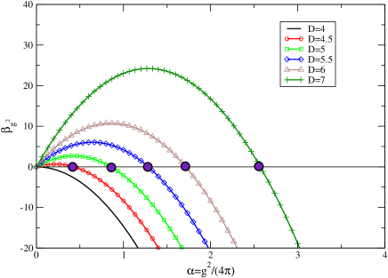
In fact, it was noted long ago [9] that the dimensionless rescaled gauge coupling, , where denotes an RG momentum scale, exhibits a non-Gaußian UV fixed point for SU() gauge theories in an expansion,
| (2) |
where has to be assumed. The UV fixed point of the coupling, being a zero of the function with negative slope, can be found at , see Fig. 1. The existence of the UV fixed point is a simple consequence of the purely dimensional running, implying a positive term , and asymptotic freedom in four dimensions, i.e., a negative term . The fixed point can be associated with a second-order phase transition between a deconfined and a “confining” phase222Whether or not standard confinement criteria are truly satisfied in the “confining” phase in has, of course, not yet been checked.. At the fixed point, the continuum limit can be taken, yielding a renormalized theory. The dimensionful renormalized coupling is asymptotically free, for increasing momentum scale , and the static quark potential becomes proportional to , independent of the dimensionality [9]. Obviously, these results are not trustworthy for five dimensions, with , and beyond, where the fixed-point coupling is large.
The lesson to be learned is that the question of renormalizability of extra-dimensional gauge theories is nonperturbative in nature, and perturbative power-counting arguments are simply useless. To answer this question, a number of lattice studies have been performed in [10, 11, 12, 13, 14], but no real evidence for a non-Gaußian fixed point has been found (we will comment on these studies in more detail below). This puts the relevance of the expansion for even more into question.
Incidentally, the UV fixed points which are discussed in the context of “GUT precursors” [15] are the direct analogue of the UV fixed point of the expansion with the contribution of the extra-dimensional modes taken into account (here the RG scale is related to the number of Kaluza-Klein modes contributing to the flow). It has been argued that the perturbative expansion parameter can be small even at the fixed point if the gauge group is sufficiently large. This would justify the use of perturbation theory and consequently the existence of the fixed point. However, as a caveat, let us remark that the smallness of the expansion parameter is not sufficient for perturbativity. For instance, the anomalous dimension at the non-Gaußian fixed point will always be large (cf. below), independent of the smallness of the fixed-point value itself. Such large anomalous dimensions have a strong influence on, e.g., the form of the effective gluon propagator [8, 16].
In section 2, we perform a nonperturbative analysis of the RG flow of gauge theories in without the need of small or . But even without this quantitative tool, a qualitative scenario can be developed which relies on a few physical prerequisites. As is apparent from the expansion Eq. (2) but also valid beyond, the function will always have the structure
| (3) |
where is the quantum-fluctuation-induced part. For small coupling, its expansion has the form, , with being the analogue of the one-loop coefficient which will generally depend on .333Contrary to , the first function coefficients are not universal in , but depend on the regularization scheme. Instead, a universal object is, e.g., the “critical exponent” . In the expansion, the nonuniversal terms appear at order and are not displayed in Eq. (2). As we will show below within the exact RG framework, the statement holds, independent of the regulator. From this, we deduce that a non-Gaußian UV fixed point exists if for some . For instance, such a fixed point always exists if is unbounded from below, as is the case to lowest order in the expansion.
Let us now assume that is a smooth function of , such that its functional form remains qualitatively similar to at least for a small number of extra dimensions (this will indeed be a result of our calculation in Sect. 2). As an analogue, one may think of dimensionally regularized amplitudes with divergencies already subtracted but with full dependence on retained. As a first guess, it is tempting to conjecture that a UV fixed point always exists in this case. This is because in , the gauge coupling is frequently expected to diverge in the infrared at a “confinement scale”. This would be a natural consequence of being unbounded from below with similar implications for .
However, the situation is more subtle because of the inherent dependence of the running coupling on its nonperturbative definition. Here, we are interested in the UV behavior of gauge-invariant operators that are building blocks of the effective action, and we expect possible non-Gaußian fixed points to be related to low-dimensional operators. Hence, we have to look at the running of those couplings which are prefactors of whole operators such as, e.g., ; by contrast, the running coupling defined, e.g., by the three-gluon vertex at various momenta would be useless, because infinitely many (derivative) operators can contribute to such a coupling. An expansion in terms of low-dimensional operators suggests the study of a Wilsonian effective action (within a gauge-invariant formalism, as used below,) of the form
| (4) |
where is the scale at which we consider the theory with all fluctuations with momenta already integrated out; the dependence of the wave function renormalization and the generalized couplings on has been displayed explicitly. A useful definition of the dimensionless running gauge coupling now is
| (5) |
such that a non-Gaußian UV fixed point in corresponds to a renormalizable operator . Further UV fixed points may exist in other couplings corresponding to further renormalizable operators which then form the UV critical surface of RG trajectories hitting the UV fixed point as we send the cutoff to infinity, .
The running of the couplings depend also on the regularization. Working with the exact renormalization group, we will use a regulator that acts as a mass term for modes with momenta smaller than but vanishes for the high-momentum modes larger than . Studying the flow of couplings with respect to a variation of allows to probe the quantum system at different momentum scales. The exact RG hence provides for a natural setting to address the question of renormalizability, i.e., the behavior of the couplings for . The regularization technique is particularly advantageous for the description of decoupling of massive modes. For a given RG cutoff scale , only particles with masses can contribute to the RG flow of running couplings. Heavy particles with are already integrated out and no modes are left that could possibly drive the flow.
In Yang-Mills theories, we are certain to encounter a mass gap in the spectrum of gluonic fluctuations. Therefore, once our RG cutoff scale has dropped below the Yang-Mills mass gap in the infrared, no fluctuations are left to renormalize the couplings any further. A freeze-out of all couplings is naturally expected in the IR for these regularizations. In particular, we expect an IR fixed point for the running gauge coupling in , with (not to be confused with the desired UV fixed point for ), see Fig. 2.
Finally assuming that for exhibits qualitatively the same functional form as in , we arrive at the following scenario. Owing to the dimensional scaling , the function starts out positive for small , such that the Gaußian fixed point is always IR attractive in . For sufficiently small , the non-Gaußian IR fixed point persists as the analogue of in . In addition to that, a non-Gaußian UV fixed point arises in between, which is the alter ego of the fixed point of the expansion. But contrary to the expansion, the non-Gaußian fixed points exist only up to a critical dimension . Beyond , the strong dimensional running simply wins out over the fluctuation-induced running, and the non-Gaußian fixed points vanish. This scenario is sketched in Fig. 2. As a result, we expect that extra-dimensional Yang-Mills theory is truly nonrenormalizable for . But the gauge theories with a non-Gaußian UV fixed point for are strong candidates for nonperturbatively renormalizable fundamental field theories.
Therefore, this scenario has the potential to solve the long-standing contradiction between the expansion and the lattice results. The crucial quantity is the size of and, in particular, whether , which would rule out extra-dimensional gauge models based purely on quantum field theory.
In the next section, an estimate for will be derived within the framework of the exact renormalization group. These results will be summarized and discussed in Sect. 3.
2 RG flow of gauge theories in extra dimensions
Our quantitative investigation is based on an exact RG flow equation for the effective average action [17] evaluated within a truncation which is discussed in detail in [18]. Here, we briefly summarize the main ingredients and focus on the generalization to dimensions.
The RG flow equation describes the evolution of the effective average action which governs the physics at a scale . The effects of all quantum fluctuations with momenta ranging from the UV down to are already included in , whereas the modes from to zero still have to be integrated out. The flow equation can formally be written as
| (6) |
where denotes the second functional derivative of , corresponding to the inverse exact propagator at the scale . The momentum-dependent mass-like regulator specifies the details of the regularization.The solution of Eq. (6) gives an RG trajectory that interpolates between the microscopic bare UV action, , and the full quantum effective action , the 1PI generating functional.
Since Eq. (6) is equivalent to an infinite tower of coupled first-order differential equations, we usually have to rely on approximate solutions of a subset of this infinite tower. A powerful tool is the method of truncations in which we restrict the effective action to a limited number of operators that are considered to be the most relevant ones for a given physical problem. In [18, 19], a truncation of the form
| (7) |
was advocated. This truncation still includes infinitely many operators, , with corresponding couplings , but is simple enough to be dealt with. Although a quantitative influence of further operators not contained in Eq. (7) has to be expected, this truncation has demonstrated its capability of controlling strong-coupling phenomena in at least qualitatively [18].
In addition to the gauge-invariant gluonic operators in Eq. (7), we include the standard ghost and gauge-fixing terms, but neglect any non-trivial running in this sector. We choose the background-field gauge and its adaption to the flow-equation formalism [20].444For the flow equation in covariant gauges, see also [21]; for the contruction of a flow-equation formalism based on gauge-invariant variables, we refer to [22]. As an important ingredient, we use a regulator , which adjusts itself to the spectral flow of in order to account for a possible strong deformation of the fluctuation spectrum in the nonperturbative domain [18, 23]. For a detailed discussion of all explicit and implicit approximations and optimizations used in this work, see [18].
Inserting this truncation into the flow equation (6) leads to a differential equation for the function , which may symbolically be written as
| (8) |
where the extensive functional depends on derivatives of , on the bare coupling , and on the anomalous dimension
| (9) |
Here we have identified , cf. Eq. (4) (a propertime-integral representation of is given in Eq. (29) of [18]). The definition (5) of the running coupling implies for the function,
| (10) |
such that we can identify . A non-Gaußian fixed point exists if for . In the language of naive RG power-counting, the anomalous dimension of the gauge field has to become large enough to turn the gauge-field interactions from “irrelevant” to “marginal” or “relevant” in .
Equation (8) is still an extremely complicated equation, and even numerical solutions will require strong analytical guidance. Therefore, we concentrate on the lowest-order term , from which we can deduce the running coupling. At this point, it should be stressed that the spectrally adjusted regulator used in this work strongly entangles the flows of the single couplings . As discussed in [18], a consistent expansion requires that the flows of contribute to the running coupling even if themselves are dropped in the end.555Neglecting the flows of leads to an unphysical pole in the anomalous dimension, for , which, if taken seriously, would induce a non-Gaußian UV fixed point for all [19]. This results in an “all-order” coupling expansion for the anomalous dimension of the form (see Eq. (40) of [18])
| (11) |
where the coefficients depend on the dimension , the number of colors , and the details of the shape function of the regulator ; this shape function has to satisfy for and should be positive and drop off sufficiently fast for in order to provide for proper IR and UV regularizations but is otherwise arbitrary. It is instructive to take a closer look at the one-loop term, i.e., the term of Eq. (11):
| (12) |
For , we find because the integrand is a total derivative and fixed to at the lower bound. Hence, we rediscover the correct one-loop function coefficient which is universal, i.e., independent of the regulator in , as expected. By contrast, this coefficient does depend on the regulator for which signals the scheme-dependence of the higher-dimensional function already to lowest order in the fluctuations; however, for all admissible regulators, this function coefficient is negative and therefore a universal property, justifying our claim in footnote 3. In the following, we employ an exponential regulator shape function which is commonly used and for which the two-loop coefficient in our approximation is reproduced to within 99% for SU(2).
It turns out that the expansion (11) is asymptotic and the coefficients grow stronger than factorially. This does not come as a surprise, since small-coupling expansions in field theory are expected to be asymptotic expansions. Moreover, since the expansion is derived from a finite integral representation of the functional in Eq. (8), we know that a finite integral representation for this asymptotic series must exist. From the method of Borel resummation [24], it is well known that good approximations of the desired integral representation can be obtained by taking only the leading growth of the coefficients into account. This program has successfully been performed in [18] for , which we generalize to in Appendix A. The finite resummed integral representation of the anomalous dimension resulting from the leading- and subleading-growth coefficients of the series (11) can be found in Eqs. (A.3,A.5,A.8). As asserted in the introduction, the fluctuation-induced contribution to the function varies smoothly as a function of , and its properties remain qualitatively the same for not too far from 4.
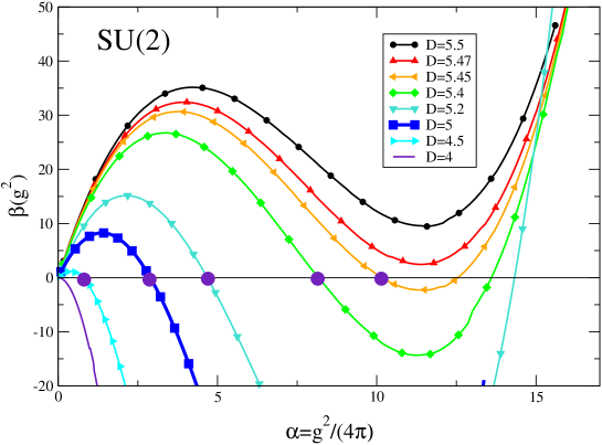
For SU(2), the function is displayed in Fig. 3 for increasing , confirming the scenario developed in the introduction. A non-Gaußian UV fixed point is found for dimensions with
| (13) |
Beyond , the function remains strictly positive and the dimensional running wins out over the fluctuation-induced running.
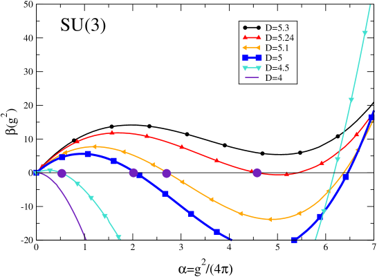
For SU(3), we are not able to resolve the full color structure completely. Therefore, we simply compute the function by scanning the whole Cartan subalgebra, as described in Appendix A and B. The error introduced by this strategy is rather small in the coupling region of interest (). Figure 4 depicts our numerical results, and we identify the critical dimension as
| (14) |
where the uncertainty arises from the unresolved color structure. The value of the critical dimension as well as the value of the non-Gaußian fixed point in a given dimension decrease with increasing . We expect this behavior to persist for higher gauge groups. For instance, we located the critical dimension at for SU(5) (the unresolved color structure inhibits a more precise estimate).
3 Conclusions
The Wilsonian approach to renormalization allows us to replace the restrictive concept of perturbative renormalizability by Weinberg’s principle of asymptotic safety. A theory is asymptotically safe if its RG flow is characterized by a finite number of ultraviolet fixed points. Whereas perturbative renormalization requires these fixed points to be Gaußian, non-Gaußian fixed points can equally serve for a continuum definition of quantum field theories. These theories are as predictive and as fundamental as their perturbatively renormalizable counterparts, and the finite number of UV fixed points determines the number of physical parameters.
We have searched for non-Gaußian UV fixed points in perturbatively nonrenormalizable (4)-dimensional Yang-Mills theories, since the prospect of a fundamental extra-dimensional quantum field theory without the need of a penumbral embedding in a larger framework is promising. Assuming a smooth dependence of the fluctuation effects on and employing the Wilsonian idea of integrating fluctuations momentum shell by momentum shell, we have developed a simple scenario for possible renormalizability. Already on a heuristic level, this scenario suggests the existence of a critical dimension below which a non-Gaußian fixed point exists and nonperturbative renormalizability is possible.
We have computed by quantizing the systems with the aid of a nonperturbative RG flow equation for the effective average action. Whereas this technique is equivalent to perturbation theory if expanded around the Gaußian fixed point, it moreover allows for an exploration of a possible non-Gaußian fixed point structure which is inaccessible to perturbation theory. In other words, the RG flow equation can be used to search for a quantizable microscopic action. In practice, this search is performed within an ansatz – a truncation – which should contain the RG “relevant” operators. In this work, we have explored a truncation based on an arbitrary function of the square of the non-abelian field strength, . Even though we have not extracted the RG behavior of the complete function , we have determined the function for the running coupling from the term linear in . Apart from the Gaußian fixed point which is IR attractive in , we find a non-Gaußian UV fixed point of the dimensionless gauge coupling as long as with
| (15) |
where the uncertainty arises from an unresolved color structure.
The fact that for all cases studied in this work, SU(), appears to point to the possibility that (=5)-dimensional Yang-Mills theories can be asymptotically safe and renormalizable. But in view of the number of approximations involved, improvements are expected to modify these results quantitatively such that strictly should not be rated as a firm prediction. At least for intermediate values of the coupling, quantitative improvements are expected from additional low-dimensional operators such as those displayed in Eq. (4). By analogy to the (=4)-dimensional case, one may argue that such additional operators contribute positively to the fluctuation part of the function, decreasing the value of .
This leads us to the conservative viewpoint that the UV fixed points observed in (=5)-dimensional Yang-Mills theory are likely to be an artifact of the approximation, and the computed values for should be considered as upper bounds. This conclusion is compatible with (most of the) lattice simulations available for : in [10, 11, 12], extra-dimensional lattice gauge systems were found to have a weak-coupling “spin-wave” and a strong-coupling “confinement” phase separated by a first-order phase transition. The latter does not allow for a continuum limit that would give rise to a renormalizable quantum field theory.666In [13], evidence for a continuum limit in (=5)-dimensional Yang-Mills theory with compactified extra dimension was found, provided that the compactification radius was small enough. However, as pointed out in [14], the asymmetric lattices in those works correspond to “extra-dimensional” lattice sites on symmetric lattices. Therefore, the continuum limit investigated in [13] seems to resemble the “deconstruction” models [25] rather than continuum extra-dimensional models. Moreover, it would be hard to understand why a compact, but still rather “macroscopical” size of the fifth dimension should modify the behavior of the theory in the deep UV.
In contrast to the conservative viewpoint, there is yet another alternative explanation for our observation of a non-Gaußian fixed point in . It may be that this fixed point for the running coupling reflects only a one-dimensional projection of a higher-dimensional critical surface . In other words, there might be a true non-Gaußian fixed point with a larger number of non-Gaußian UV attractive components corresponding to a number of RG “relevant” operators. Since our calculation also involves higher-order operators , our truncation could be sensitive to the influence of these operators stabilizing the UV fixed point of the coupling. This would not necessarily be in contradiction to the lattice results which have only employed the Wilson action or small modifications thereof.777Only in [12], two higher-order operators have been included with a negative result for an UV fixed point. But since this result applies to and SU( or ) lattice gauge theory, it is in perfect agreement with our investigation. If the Wilson action is not in the domain of attractivity of the true fixed point, i.e., in the same universality class as the renormalizable action, the line of “constant physics” towards the continuum limit will not be visible on the lattice. If this second alternative turned out to be true, a purely field theoretic fundamental and renormalizable extra-dimensional model could be constructed, but a larger number of physical parameters would have to be fixed for the model to be predictive. For a detailed investigation of this issue, a systematic inclusion of all low-dimensional operators such as those displayed in Eq. (4) seems mandatory. As a final caveat, let us mention that, even if such a renormalizable theory existed, it would not be immediate that its compactified low-energy limit is effectively four-dimensional and confining.
Up to now, we have only focused on pure gauge theory. In fact, we believe that this is the most stringent test for the existence of a non-Gaußian fixed point in . Matter fields are expected to make positive contributions to the function, thus lifting the curves and decreasing . We do not have a full nonperturbative proof for this, but this tendency is clearly observed in perturbation theory even to higher loop orders. As a first guess, we have included a fundamental quark loop with flavors in the calculation, and observed that all ’s dropped below 5, except for the case of SU(2) and , where stays slightly larger than . If this tendency also holds for more reliable computations, extra-dimensional systems with the full standard-model particle content will not be nonperturbatively renormalizable.
Let us finally comment on the effects of compactification, which relates the effective four-dimensional low-energy theory to the extra-dimensional theory, be it renormalizable or not. During the transition from low-energy, , to high-energy scales, , separated by the inverse compactification radius , the function is explicitly dependent on . Pictorially, this function interpolates between the curve and the corresponding curve for increasing in a smooth fashion that depends on the details of the boundary conditions. (The ascending curves of Fig. 2 may also be viewed as snapshots of for increasing .) Starting from the four-dimensional low-energy theory, the coupling first gets weak for increasing , owing to asymptotic freedom. As soon as the extra dimensions become “visible” due to the fluctuations of the lowest Kaluza-Klein modes, the positive term appears effectively in together with the non-Gaussian UV fixed point. Hence, the coupling grows stronger and quickly approaches the UV fixed point value. Since the function itself changes its shape with increasing , the UV fixed point moves to larger values and so does the coupling. If the theory is renormalizable, , the UV fixed point remains and marks the limiting value of the dimensionless coupling. If the theory is nonrenormalizable, , the fixed point vanishes and the coupling will eventually hit a Landau pole, signaling the onset of “new physics”. As is obvious from this discussion, a non-Gaussian UV fixed point does exist at least for intermediate scales , even in the nonrenormalizable case. Although this “freezes” the coupling at the intermediate scales, it does not help to separate the compactification scale far from the scale of new physics in the nonrenormalizable case, since the UV fixed point vanishes as soon as , and the coupling will generally grow quickly. As a consequence, this line of argument may serve to exclude extra-dimensional models with perturbative gauge-coupling unification at a high scale GeV, but low-scale extra dimensions separated by many orders of magnitude, .
Acknowledgment
The author is grateful to R. Hofmann, J. Jaeckel, U.D. Jentschura, J.M. Pawlowski, Z. Tavartkiladze and C. Wetterich for useful discussions and J.M. Pawlowski for detailed comments on the manuscript. The author acknowledges financial support by the Deutsche Forschungsgemeinschaft under contract Gi 328/1-2.
Appendix
A Resummation of the anomalous dimension
In this appendix, we list some details of the calculation of the anomalous dimension, taking the leading growth of the coefficients of the series (11) into account. The following formulas should be read side-by-side with the calculations given in [18].
These leading-growth (l.g.) coefficients read for ,
| (A.1) | |||||
where we abbreviated , and are the Bernoulli numbers. Actually, Eq. (A.1) also contains subleading terms, since the last term is negligible compared to the term for large . Nevertheless, we also retain this subleading term, since it contributes significantly to the one-loop function coefficient which we want to maintain in our approximation. Let us first concentrate on SU(2), where the color factor for all (for its definition, see Appendix B); let us nevertheless retain the dependence in all other terms in order to facilitate the generalization to higher gauge groups. The scheme-dependent coefficient can be represented by
| (A.2) | |||||
for the exponential regulator shape function. The last equality holds only for , which will be sufficient for our purposes.888For larger extra dimensions, valid representations can be found by partial integration of the integral. The remaining resummation is performed similarly to [18]: we split the anomalous dimension into two parts,
| (A.3) |
where corresponds to the resummation of the term , and to the term in Eq. (A.1), representing the leading and subleading growth, respectively. For resumming , we use the standard integral representation of the functions, such that all dependent terms lead to the sum
| (A.4) |
The first sum is strictly valid only for ; however, the second sum is valid for arbitrary , apart from simple poles at , and rapidly converging, so that this equation should be read from right to left. With this definition, the leading-growth part of the anomalous dimension can be written as
| (A.5) | |||||
where the auxiliary functions , are defined as
| (A.6) |
and is the modified Bessel function. For resumming the subleading-growth part , we use an integral representation of the Euler Beta function for the ratio of functions, and the resulting sum can be transformed analogously to Eq. (A.4), yielding
| (A.7) |
where we abbreviated . The subleading-growth part of the anomalous dimension finally reads
| (A.8) |
where and . In arriving at Eq. (A.8), we implicitly used a principal-value prescription for the poles of on the negative axis. This has been physically motivated in [18] and moreover agrees with systematic studies of the resummation procedure [26].
Both integral representations in Eqs. (A.5), (A.8) are finite, can be evaluated numerically, and reproduce the asymptotic-series coefficients of Eq. (A.1) upon expansion in . For , they agree with the results of [18].
For the gauge group SU(3), we do not have the explicit representation of the color factors at our disposal. As discussed in Appendix B, we instead scan the Cartan sub-algebra for the possible range of the . Inserting the extrema or as found in Eq. (B.4) into Eq. (A.1) allows us to display the anomalous dimension in terms of the formulas deduced for SU(2):
| (A.9) |
The notation here indicates that the quantities and appearing on the right-hand sides of Eqs. (A.5) and (A.8) should be replaced in the prescribed way. The SU(5)-case works similarly with the help of Eq. (B.5).
B Color factors
Gauge group information enters the flow equation via color traces over products of field strength tensors and gauge potentials. For the calculation within the present truncation, it suffices to consider these quantities as pseudo-abelian, pointing into a constant color direction . In this case, the color traces reduce to
| (B.1) |
where the parentheses at the color indices denote symmetrization. For general gauge groups, these factors are not independent of the direction of . Contrary to this, the left-hand side of the flow equation is a function of which is independent of . Therefore, we do not need the complete factor of Eq. (B.1), but only that part of the symmetric invariant tensor which is proportional to the trivial one,
| (B.2) |
where we omitted further nontrivial symmetric invariant tensors. The latter do not contribute to the flow of , but to that of other operators which do not belong to our truncation. For the gauge group SU(2), all complications are absent, since there are no further symmetric invariant tensors in Eq. (B.2), implying
| (B.3) |
For higher gauge groups, we do not evaluate the ’s from Eq. (B.2) directly; instead, we explore the possible values of the whole trace of Eq. (B.1) for different choices of . For this, we exploit the fact that the color unit vector can always be rotated into the Cartan sub-algebra. For SU(3), we choose a color vector pointing into the 3 or 8 direction in color space, representing the two possible extremal cases for which the trace boils down to
| (B.4) |
We follow the same strategy for SU(5), where the color factors for the 3,8,15, and 24 direction reduce to
| (B.5) |
The uncertainty introduced by the artificial dependence of the color factors is responsible for the uncertainties of our results for the SU(3) and SU(5) critical dimension . Obviously, the uncertainty increases with the size of the Cartan sub-algebra, i.e., the rank of the gauge group.
References
-
[1]
I. Antoniadis,
Phys. Lett. B 246, 377 (1990);
A. Pomarol and M. Quiros, Phys. Lett. B 438, 255 (1998) [arXiv:hep-ph/9806263];
K. R. Dienes, E. Dudas and T. Gherghetta, Nucl. Phys. B 537, 47 (1999) [arXiv:hep-ph/9806292]; arXiv:hep-ph/9807522. -
[2]
Y. Kawamura,
Prog. Theor. Phys. 103, 613 (2000)
[arXiv:hep-ph/9902423];
G. Altarelli and F. Feruglio, Phys. Lett. B 511, 257 (2001) [arXiv:hep-ph/0102301]; - [3] S. Weinberg, in C76-07-23.1 HUTP-76/160, Erice Subnucl. Phys., 1, (1976).
- [4] K. G. Wilson, Phys. Rev. D 7, 2911 (1973).
-
[5]
B. Rosenstein, B. J. Warr and S. H. Park,
Phys. Rev. Lett. 62, 1433 (1989);
K. Gawedzki and A. Kupiainen, Phys. Rev. Lett. 55, 363 (1985);
C. de Calan, P. A. Faria da Veiga, J. Magnen and R. Seneor, Phys. Rev. Lett. 66, 3233 (1991). -
[6]
O. Lauscher and M. Reuter,
Phys. Rev. D 65, 025013 (2002)
[arXiv:hep-th/0108040]; Class. Quant. Grav. 19, 483 (2002)
[arXiv:hep-th/0110021];
W. Souma, Prog. Theor. Phys. 102, 181 (1999) [arXiv:hep-th/9907027];
R. Percacci and D. Perini, Phys. Rev. D 67, 081503 (2003) [arXiv:hep-th/0207033];
P. Forgacs and M. Niedermaier, arXiv:hep-th/0207028. - [7] N. Seiberg, Phys. Lett. B 388, 753 (1996) [arXiv:hep-th/9608111]; Phys. Lett. B 390, 169 (1997) [arXiv:hep-th/9609161].
- [8] D. I. Kazakov, arXiv:hep-th/0209100.
- [9] M. E. Peskin, Phys. Lett. B 94, 161 (1980).
- [10] M. Creutz, Phys. Rev. Lett. 43, 553 (1979) [Erratum-ibid. 43, 890 (1979)].
- [11] H. Kawai, M. Nio and Y. Okamoto, Prog. Theor. Phys. 88, 341 (1992).
- [12] J. Nishimura, Mod. Phys. Lett. A 11, 3049 (1996) [arXiv:hep-lat/9608119].
-
[13]
S. Ejiri, J. Kubo and M. Murata,
Phys. Rev. D 62, 105025 (2000)
[arXiv:hep-ph/0006217];
S. Ejiri, S. Fujimoto and J. Kubo, Phys. Rev. D 66, 036002 (2002) [arXiv:hep-lat/0204022]. - [14] K. Farakos, P. de Forcrand, C. P. Korthals Altes, M. Laine and M. Vettorazzo, Nucl. Phys. B 655, 170 (2003) [arXiv:hep-ph/0207343].
-
[15]
K. R. Dienes, E. Dudas and T. Gherghetta,
arXiv:hep-th/0210294;
F. Paccetti Correia, M. G. Schmidt and Z. Tavartkiladze, arXiv:hep-ph/0302038. - [16] N. V. Krasnikov, Phys. Lett. B 273, 246 (1991).
-
[17]
C. Wetterich,
Phys. Lett. B 301, 90 (1993);
Nucl. Phys. B 352, 529 (1991);
for a review, see J. Berges, N. Tetradis and C. Wetterich, arXiv:hep-ph/0005122;
D. F. Litim and J. M. Pawlowski, arXiv:hep-th/9901063. - [18] H. Gies, Phys. Rev. D 66, 025006 (2002) [arXiv:hep-th/0202207].
- [19] M. Reuter and C. Wetterich, Phys. Rev. D 56, 7893 (1997) [arXiv:hep-th/9708051].
-
[20]
M. Reuter and C. Wetterich,
Nucl. Phys. B 417, 181 (1994);
F. Freire, D. F. Litim and J. M. Pawlowski, Phys. Lett. B 495, 256 (2000) [arXiv:hep-th/0009110]. -
[21]
M. Bonini, M. D’Attanasio and G. Marchesini,
Nucl. Phys. B 421, 429 (1994)
[arXiv:hep-th/9312114];
U. Ellwanger, Phys. Lett. B 335, 364 (1994) [arXiv:hep-th/9402077]. -
[22]
T. R. Morris,
Nucl. Phys. B 573, 97 (2000)
[arXiv:hep-th/9910058];
S. Arnone, A. Gatti and T. R. Morris, Phys. Rev. D 67, 085003 (2003) [arXiv:hep-th/0209162]. - [23] D. F. Litim and J. M. Pawlowski, Phys. Rev. D 66, 025030 (2002) [arXiv:hep-th/0202188]; Phys. Lett. B 546, 279 (2002) [arXiv:hep-th/0208216].
-
[24]
G. Hardy, “Divergent Series,” Oxford Univ. Press (1949);
C.M. Bender and S.A. Orszag, “Advanced Mathematical Methods for Scientists and Engineers,” McGraw-Hill, New York (1978). -
[25]
N. Arkani-Hamed, A. G. Cohen and H. Georgi,
Phys. Rev. Lett. 86, 4757 (2001)
[arXiv:hep-th/0104005];
C. T. Hill, S. Pokorski and J. Wang, Phys. Rev. D 64, 105005 (2001) [arXiv:hep-th/0104035]. -
[26]
U. D. Jentschura, E. J. Weniger and G. Soff,
J. Phys. G 26, 1545 (2000)
[arXiv:hep-ph/0005198];
U. D. Jentschura, habilitation thesis, Dresden Tech.U. (2002).