Phantom with Born-Infeld type Lagrangian

Abstract

ABSTRACT: Recent analysis of the observation data indicates that the equation of state of the dark energy might be smaller than $-1$, which leads to the introduction of phantom models featured by its negative kinetic energy to account for the regime of equation of state $w<-1$. In this paper, we generalize the idea to the Born-Infeld type Lagrangian with negative kinetic energy term and give the condition for the potential, under which the late time attractor solution exists and also analyze a viable cosmological model in such a scheme.

1. Introduction

More and more astronomical observations converge on that about two thirds of the energy density in our universe is resulted from dark energy that has negative pressure and can drive the accelerating expansion of the universenewobservation . Many candidates for dark energy have been proposed so far to fit the current observations. Among these models, the most important ones are cosmological constant and a time varying scalar field evolving in a specific potential, referred to as ”quintessence”steinhardt . The major difference among these models are that they predict different equation of state of the dark energy and thus different cosmology. Especially, for these models, the equations of state are confined within the range of $-1<w<-1/3$, which can drive the accelerating expansion of the universe. However, some analysis to the observation data hold that the range of the equation of state may not always be greater than $-1$, in fact, they can lie in the range $-1.38<w<-0.82$melchiorri . Especially, the new results from SN-Ia alone are suggesting $w<-1$ at 1 $\sigma$tonry . It is obvious that the equation of state of conventional quintessence models that based on a scalar field with positive kinetic energy can not evolve to the the regime of $w<-1$, and therefore, some authorscaldwell1 ; sahni ; parker ; chiba ; boisseau ; schulz ; faraoni ; maor ; onemli ; torres ; carroll ; frampton ; hao ; caldwell2 ; gibbons ; feinstein investigated phantom field models that possess negative kinetic energy and can realize $w<-1$ in their evolution. It is true that the field theory with negative kinetic energy poses a challenge to the widely accepted energy condition and leads to rapid vacuum decaycarroll , but it is still very interesting to study these models in the sense that it is phenomenologically interesting.

On the other hand, the role of rolling tachyon in string theory in cosmology has been widely studiedtachyon . It is shown that the tachyon can be described by a Born-Infeld (B-I) type Lagrangian with a specific potential resulted from string theory. However, it is known that the tachyon field is not suitable for driving the late time accelerating expansion of the universe because the dynamical evolution does not admit a late time attractor solutionli . In this paper, we combine the two ideas together and introduce the negative kinetic energy term to the B-I type Lagrangian and investigate its cosmological evolution. We firstly study the B-I type phantom model in an arbitrary potential and give the condition for the potential to admit a late time attractor solution that corresponds to the equation of state $w=-1$ and then work in a specific viable model. We also demonstrate that current universe is not a stable stage in such a model while is in its way to the stable stage, at which the universe is dominated by the vacuum energy like dark energy with a equation of state of $-1$.

2. The Phantom Model With B-I Lagrangian

Although there exist a number of impressive calculations of the phantom field, yet the precise Lagrangian is not completely known at present. Among the many models that have been proposed to account for the dark energy in the universe, k-essence is the most general formgibbons , in which the lagrangian is expressed as $L=L(\phi,y)$, where $y=\frac{1}{2}g^{\mu\nu}\partial_{\mu}\phi\partial_{\nu}\phi$. Sen’s tachyon theory corresponds to the choice of Lagrangian as $L=-V(\phi)\sqrt{1+2y}$. Gibbonsgibbons1 has argued that there are many objections to a naive inflationary model based on the tachyon, but there remains the possibility that the tachyon was important in a possible pre-inflationary ”open-string era” preceding our present ”closed-string ear”. In this paper, we consider the case that the kinetic energy term is negative

$$L=-V(\phi)\sqrt{1-2y}$$ (1)

in the spatially flat Robertson-Walker metric,

$$ds^{2}=-dt^{2}+a^{2}(t)(dx^{2}+dy^{2}+dz^{2})$$ (2)

Then for the spatially homogeneous scalar field, we have the following Lagrangian

$$L=-V(\phi)\sqrt{1+\dot{\phi}^{2}}$$ (3)

where $V(\phi)$ is the potential of the model. When we consider the phantom field $\phi$ dominant era, the Einstein equations for the evolution of the background metric,$G_{\mu\nu}=\kappa T_{\mu\nu}$ can be written as:

$$H^{2}=(\frac{\dot{a}}{a})^{2}=\frac{\kappa}{3}\rho_{\phi}$$ (4)

and

$$\frac{\ddot{a}}{a}=-\frac{\kappa}{3}(\frac{1}{2}\rho_{\phi}+\frac{3}{2}p_{\phi})$$ (5)

For a spatially homogenous phantom field $\phi$, we have the equation of motion

$$\ddot{\phi}+3H\dot{\phi}(1+\dot{\phi}^{2})-\frac{V^{{}^{\prime}}(\phi)}{V(\phi)}(1+\dot{\phi}^{2})=0$$ (6)

where the over dot represents the differentiation with respect to $t$ and the prime denotes the differentiation with respect to $\phi$. Eq.(6) is also equivalent to the entropy conservation equation. The constant $\kappa=8\pi G$ where $G$ is Newtonian gravitation constant. The density $\rho_{\phi}$ and the pressure $p_{\phi}$ are defined as following:

$$\rho_{\phi}=\frac{V(\phi)}{\sqrt{1+\dot{\phi}^{2}}}$$ (7)

$$p_{\phi}=-V(\phi)\sqrt{1+\dot{\phi}^{2}}$$ (8)

the equation of state is

$$w_{\phi}=\frac{p_{\phi}}{\rho_{\phi}}=-\dot{\phi}^{2}-1$$ (9)

It is clear that the equation of state $w$ will be less than $-1$ unless the kinetic energy term $\dot{\phi}^{2}=0$.

3. Dynamical Evolution of Phantom Field

In this section, we investigate the global structure of the dynamical system via phase plane analysis and compute the cosmological evolution by numerical analysis. Firstly, we consider the evolution when the phantom field becomes dominant and thus neglect the non-relativistic and relativistic components (matter and radiation) in the universe. Then, from Eq.(4) and (6), we have

$$\ddot{\phi}+\sqrt{3\kappa}\dot{\phi}\left[\frac{V(\phi)}{\sqrt{1+\dot{\phi}^{2}}}\right]^{1/2}(1+\dot{\phi}^{2})-\frac{V^{{}^{\prime}}(\phi)}{V(\phi)}(1+\dot{\phi}^{2})=0$$ (10)

To gain more insight into the above equation while not lose generality, we here do not specify the potential. Introducing the new variables

$$X=\phi$$ (11)

$$Y=\dot{\phi}$$

then Eq.(10) becomes

$$\frac{dX}{dt} =Y$$ (12)

$$\frac{dY}{dt} =(1+Y^{2})\frac{V^{\prime}}{V}-\sqrt{3V\kappa}(1+Y^{2})^{3/4}Y$$

Linearize the above equation around its critical point $(X_{c},0)$, one obtain that

$$\frac{dX}{dt} =Y$$ (13)

$$\frac{dY}{dt} =\frac{V^{\prime\prime}(X_{c})}{V(X_{c})}X-\sqrt{3V(X_{c})\kappa}Y$$

where the critical value of $X$ is determined by $V^{\prime}(X_{c})=0$. The types of the critical point is determined by the eigenequation of the system

$$\lambda^{2}+\alpha\lambda+\beta=0$$ (14)

where $\alpha=\sqrt{3V(X_{c})}\kappa$ and $\beta=-\frac{V^{\prime\prime}(X_{c})}{V(X_{c})}$. The two eigenvalues are

$$\lambda_{1}=\frac{1}{2}\left(-\sqrt{3V(X_{c})\kappa}-\sqrt{3V(X_{c})\kappa+4\frac{V^{\prime\prime}(X_{c})}{V(X_{c})}}\right)$$ (15)

$$\lambda_{1}=\frac{1}{2}\left(-\sqrt{3V(X_{c})\kappa}+\sqrt{3V(X_{c})\kappa+4\frac{V^{\prime\prime}(X_{c})}{V(X_{c})}}\right)$$ (16)

For positive potentials, If $V^{\prime\prime}(X_{c})<0$, then the critical point $(X_{c},0)$ is a stable node, which implies that the dynamical system admits attractor solutions.

In the following, we will show this with a specific model, to do which, we must specify the potential. We choose the widely studied potential for tachyon askutasov

$$V(\phi)=V_{0}(1+\frac{\phi}{\phi_{0}})\exp(-\frac{\phi}{\phi_{0}})$$ (17)

It is not difficult to find that the critical $X_{c}=0$ and $\frac{V^{\prime\prime}(X_{c})}{V(X_{c})}=-\frac{1}{\phi_{0}^{2}}$ in such a potential. Therefore, this model has an attractor solution which corresponds to $\phi=0$, $\dot{\phi}=0$ and thus $w=-1$. Before the field evolves to its attractor regime, the equation of state $w<-1$.

Next, we solve this model via numerical approach. To do this, we firstly re-scale the quantities as $\phi=x\phi_{0}$ and $t=s\phi_{0}$. Then the Eq.(12) becomes dimensionless

$$\frac{dx}{ds} =y$$ (18)

$$\frac{dy}{ds} =-\frac{x(1+y^{2})}{1+x}-\eta y(1+y^{2})^{\frac{3}{4}}(1+x)^{\frac{1}{2}}\exp(-\frac{x}{2})$$

where $\eta=\sqrt{3V_{0}\kappa}\phi_{0}$ is a dimensionless parameter. The numerical results are plotted in Fig.1, Fig.2, Fig.3 and the parameter $\eta=2.1$.

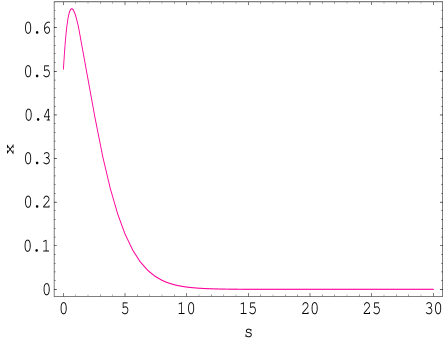
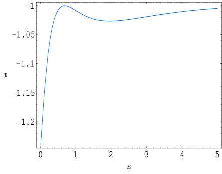
Figure 1: The evolution of the field $\phi$ with respect to $s$ when the phantom is dominant

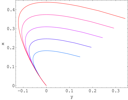
Figure 2: The evolution of the equation of state of the phantom $w$ with respect to $s$ when the phantom is dominant

Figure 3: The attractor property of the system in the phase plane when the phantom is dominant

4. Evolution of phantom at the presence of matter and radiation

In former section, we study the evolution of the phantom when it dominates over all other energy density. Now, we consider the radiation and matter density and investigate the evolution of the phantom field. The presence of radiation and matter will alter the Eq.(4) as

$$H^{2}=\frac{\kappa}{3}\left(\rho_{\phi}+\rho_{M}+\rho_{r}\right)$$ (19)

where $\rho_{M}$ and $\rho_{r}$ denote the non-relativistic and relativistic components (or matter and radiation) energy density respectively. Eq.(19) could be rewritten as

$$H^{2}=H_{i}^{2}\left(\frac{\rho_{\phi}}{\rho_{c,i}}+\Omega_{M,i}\left(\frac{a_{i}}{a}\right)^{3}+\Omega_{r,i}\left(\frac{a_{i}}{a}\right)^{4}\right)$$ (20)

where the subscript $i$ denotes the quantity at the initial time $t_{i}$. $\rho_{c,i}$ is the critical density of the universe at the initial $i$, which is defined as $\rho_{c,i}=\frac{3H_{i}^{2}}{\kappa}$. $\Omega_{M,i}$ and $\Omega_{r,i}$ are the cosmic density parameters for matter and radiation at $t_{i}$. We introduce the new dimensionless variables

$$x =\frac{\phi}{\phi_{0}}$$

$$y =\frac{d\phi}{dt}$$

$$N =\ln a$$ (21)

Then the Eq.(6) will reduce to the following equation systems

$$\frac{dx}{dN} =\frac{y}{H_{i}\phi_{0}}\xi$$

$$\frac{dy}{dN} =-3y(1+y^{2})+\frac{(1+y^{2})V^{\prime}}{H_{i}V}\xi$$ (22)

where the prime denote the differentiation with respect to $x$ and $\xi$ is defined as

$$\xi=\left[\frac{\kappa V}{3H_{i}^{2}\sqrt{1+y^{2}}}+\Omega_{M,i}\left(\frac{a_{i}}{a}\right)^{3}+\Omega_{r,i}\left(\frac{a_{i}}{a}\right)^{4}\right]^{-1/2}$$ (23)

If we specify the initial scale factor $a_{i}=1$ then we can express $\xi$ as a function of $N$

$$\xi(N)=\left[\frac{\kappa V}{3H_{i}^{2}\sqrt{1+y^{2}}}+\Omega_{M,i}e^{-3N}+\Omega_{r,i}e^{-4N}\right]^{-1/2}$$ (24)

Before we carry out the numerical study, we would like to analyze the system of equations qualitatively. When N goes to be very large, or at late time, the contribution to $H$ from matter and radiation will become negligible. Therefore, the Eq.(Phantom with Born-Infeld type Lagrangian) will reduce to

$$\frac{dx}{dN} =\sqrt{\frac{3}{\kappa}}\frac{y}{\phi_{0}}\left[\frac{\sqrt{1+y^{2}}}{V(x)}\right]^{1/2}\noindent$$ (25)

$$\frac{dx}{dN} =-3y(1+y^{2})+\sqrt{\frac{3}{\kappa}}\frac{V^{\prime}(x)}{V(x)}\left[\frac{\sqrt{1+y^{2}}}{V(x)}\right]^{1/2}(1+y^{2})$$ (26)

Note that these equations are re-expressions of the Eq.(12) in term of $N$ instead of $s$. These two different expression are essentially the same and therefore the condition for the existence of attractor solution $V^{\prime\prime}(x_{c})<0$ still hold true. Thus, from the above qualitative analysis, we can conclude that for the tachyon potential Eq.(17), there is still a late time attractor solution even if at the presence of matter and radiation.

Next, we will numerically study the system at the presence of matter and radiation in the potential(17) and obtain the results that will confirm our qualitative analysis. Substitute Eq.(17) into Eq.(Phantom with Born-Infeld type Lagrangian) we have

$$\frac{dx}{dN} =\frac{y}{H_{i}\phi_{0}}\xi^{\prime}(N)\noindent$$ (27)

$$\frac{dy}{dN} =-3y(1+y^{2})-\frac{(1+y^{2})x}{H_{i}\phi_{0}(1+x)}\xi^{\prime}(N)$$ (28)

where $\xi^{\prime}(N)$ is

$$\xi^{\prime}(N)=\left[\frac{\kappa V_{0}(1+x)e^{-x}}{3H_{i}^{2}\sqrt{1+y^{2}}}+\Omega_{M,i}e^{-3N}+\Omega_{r,i}e^{-4N}\right]^{-1/2}$$ (29)

Solving these equations will give us some insights into the evolution of the field and the quantities of interest. We specify our starting point as the equipartition epoch, at which the $\Omega_{M}=\Omega_{r}=0.5$. The results are shown in Fig.4, Fig.5, and Fig.6 (The plots are done by choosing the dimensionless parameter $\frac{\kappa V_{0}}{3H_{i}^{2}}=0.00000033$). From these results, we can conclude that the current energy density composition is not an final evolution stage in this specific model. In stead, the universe will evolve to a de Sitter like attractor regime in the future and the energy density of dark energy will become completely dominant over the non-relativistic matter ($\Omega_{\phi}\rightarrow 1$) and behave as a cosmological constant.

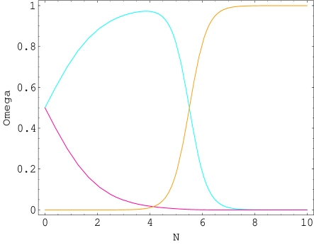
Figure 4: The evolution of the equation of state of phantom with respect to $N$ at the presence of matter and radiation. Plot begins from the equipartition epoch

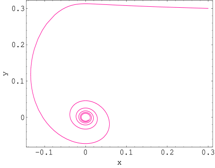
Figure 5: The evolution of $\Omega_{M}$(blue curve), $\Omega_{r}$ (red curve)and $\Omega_{\phi}$(orange curve) with respect to $N$. The plot begins from the equipartition epoch ($\Omega_{M}=\Omega_{r}$).

Figure 6: The attractor property of the phantom at the presence of matter and radiation. Plot begins from the equipartition epoch.

5. Discussion

In this paper, we study the cosmological implication of a Born-Infeld type Lagrangian with negative kinetic energy term. One may also consider this as a new realization of k-essence with an equation of state $w\leq-1$. Analysis to the dynamical evolution of the phantom model indicates that it admits a late time attractor solution, at which the field behaves as a cosmological constant. Before the field evolves to its attractor regime, the equation of state of the field is less than $-1$. In the k-essence model, the speed of sound is

$$c_{s}^{2}=\frac{p_{,X}}{\rho_{,X}}=\frac{L_{\phi,X}}{L_{\phi,X}+2XL_{\phi,XX}}$$ (30)

where $p=L_{\phi}(\phi,X)$ and $\rho=2XL_{\phi,X}-L_{\phi}(\phi,X)$ with $X=\frac{1}{2}(\partial_{\mu}\phi)^{2}$. So, the speed of sound of the phantom with B-I Lagrangian is $1+\dot{\phi}^{2}$, which means that the perturbations of the background field can travel faster than light as measured in the preferred frame where the background field is homogeneous. For a time dependent background field, this is not a Lorentz invariant state. However, it does not violate causality because the underlying theory is manifestly Lorentz invariant and it is not possible to transmit information faster than light along arbitrary space-like directions or create closed time-like curveserickson .

Up to now, the observation data do not tell us what should be the nature of dark energy. But the future observation will be helpful to determine whether the dark energy is phantom, quintessence, or cosmological constant. If the equation of state $w<-1$ is completely confirmed by observation, then its implication to fundamental physics would be astounding, since it cannot be achieved with substance with canonical Lagrangian. Phantom with B-I Lagrangian could be an interesting candidate for dark energy with an equation of state $w<-1$.

ACKNOWLEDGEMENT: We thank Alessandro Melchiorri for helpful comments. This work was partially supported by National Nature Science Foundation of China under Grant No. 19875016, and Foundation of Shanghai Development for Science and Technology under Grant No.01JC14035.

References

- (1) P. de Bernardis et al. Nature 404 955(2000); S. Hanany et al. Astrophys. J. 545 1 (2000); N. Bahcall, J. P. Ostriker, S. Perlmutter and P. J. Steinhardt Science 284 1481(1999); S. Perlmutter et al. Astrophys. J. 517 565(1999 ); A. G. Riess et al., Astron. J. 116 1009(1998)
- (2) B. Ratra and P. J. Peebles, Phys. Rev. D37 3406(1988); R. R. Caldwell, R. Dave and P. J. Steinhardt, Phys. Rev. Lett. 80 1582(1998); P. J. Steinhardt, L . Wang and I . Zlatev, Phys. Rev. D59 123504(1999); I. Zlatev, L. Wang and P. J. Steinhardt, Phys. Rev. Lett. 82 896(1999); K. Coble, S. Dodelson, J. Frieman, Phys. Rev. D55 1851(1997); X. Z. Li, J. G. Hao, D. J. Liu, Class.Quant.Grav. 19 6049(2002)
- (3) A. Melchiorri, L. Mersini, C. J. Odmann and M. Trodden, Astro-ph/0211522
- (4) J. L. Tonry et al., astro-ph/0305008
- (5) R.R. Caldwell, Phys.Lett. B545 23(2002).
- (6) V. Sahni and A. A. Starobinsky, Int. J. Mod. Phys. D9 373(2002)
- (7) L. Parker and A. Raval, Phys. Rev. D60 063512(1999)
- (8) T. Chiba, T. Okabe and M. Yamaguchi, Phys. Rev. D62 023511(2000)
- (9) B. Boisseau, G. Esposito-Farese, D. Polarski and A. A. Starobinsky, Phys. Rev. Lett.85 2236, (2000)
- (10) A. E. Schulz, Martin White, Phys.Rev. D64 043514(2001)
- (11) V. Faraoni, Int. J. Mod. Phys. D64 043514 (2002)
- (12) I. Maor, R. Brustein, J. Mcmahon and P. J. Steinhardt, Phys. Rev. D65 123003(2002)
- (13) V. K. Onemli and R. P. Woodard, Class. Quant. Grav. 19 4607(2002)
- (14) D. F. Torres, Phys. Rev. D66 043522 (2002)
- (15) S. M. Carroll, M. Hoffman, M. Trodden, astro-ph/0301273
- (16) P. H. Frampton, Stability Issues for Dark Energy, hep-th/0302007
- (17) J. G. Hao and X. Z. Li, gr-qc/0302100, to be published in Phys. Rev. D; X. Z. Li and J. G. Hao, hep-th/0303093.
- (18) R. R Caldwell, M. Kamionkowski and N. N. Weinberg, astro-ph/0302506
- (19) G. W. Gibbons, hep-th/0302199
- (20) A. Feinstein and S. Jhingan, hep-th/0304069; L. P. Chimento and A. Feinstein, astro-ph/0305007; P. Singh, M. Sami and N. Dadhich, hep-th/0305110
- (21) A. Sen, JHEP 0204, 048 (2002); A. Sen, JHEP 0207, 065(2002); G.W.Gibbons, Phys. Lett. B537, 1 (2002); M. Fairbairn and M. H. G. Tytgat, Phys.Lett.B546, 1 (2002); A. Sen J. Math. Phys. 42, 2844(2001); G. W. Gibbons, K. Hori and P. Yi, Nucl. Phys. B596, 136 (2001); A. Sen, hep-th/0303057; J. G. Hao and X. Z. Li, Phys. Rev. D66, 087301(2002); X. Z. Li and X. H. Zhai, Phys. Rev.D67, 067501(2003); A. Frolov, L. Kofman and A. Starobinsky, hep-th/0204187; S. Mukohyama, Phys. Rev. D66, 024009(2002); T. Padmanabhan, Phys. Rev. D66, 021301 (2002); M. Sami and T. Padmanabhan, Phys. Rev. D67, 083509(2003); G. Shiu and I. Wasserman, Phys. Lett. B541, 6(2002); L. Kofman and A. Linde, hep-th/020512; H. B. Benaoum, hep-th/0205140; A. Ishida and S. Uehara, hep-th/0206102; T. Chiba, astro-ph/0206298; T, Mehen and B. Wecht, hep-th/0206212; A. Sen, hep-th/0207105; N. Moeller and B. Zwiebach,JHEP 0210, 034(2002); J. M. Cline, H. Firouzjahi and P. Martineau, hep-th/0207156; S. Mukohyama, hep-th/0208094; P. Mukhopadhyay and A. Sen, hep-th/020814; T. Okuda and S. Sugimoto, hep-th/0208196; G. Gibbons , K. Hashimoto and P. Yi, hep-th/0209034; M. R. Garousi, hep-th/0209068; A. Sen, hep-th/0209122; B. Chen , M. Li and F. Lin, hep-th/0209222; J. Luson, hep-th/0209255; C. Kim, H. B. Kim, Y. Kim and O. K. Kwon, hep-th/0301142; X.Z. Li, D.J.Liu and J.G.Hao, hep-th/0207146; J.M.Cline, H. Firouzjahi and P. Martineau, hep-th/0207156; G. Felder, L. Kofman and A. Starobinsky, JHEP 0209, 026(2002); S. Mukohyama, arXiv:hep-th/0208094; G.A. Diamandis, B.C. Georgalas , N.E. Mavromatos, E. Papantonopoulos, hep-th/0203241; G.A. Diamandis, B.C. Georgalas , N.E. Mavromatos, E. Papantonopoulos, I. Pappa, hep-th/0107124; M. C. Bento, O. Bertolami and A. A. Sen,hep-th/020812; M.C. Bento, O. Bertolami., A. A. Sen, Phys.Rev. D67, 023504,2003; C. Kim , H. B. Kim and Y. Kim, hep-th/0210101; C. Kim, Y. Kim, O. K. Kwon, C. Oh Lee, hep-th/0305092 ; H. Lee, W. S. l’Yi, hep-th/0210221; J.S.Bagla, H.K.Jassal, T.Padmanabhan, astro-ph/0212198; M. Sami, P Chingangbam and T Qureshi, hep-th/0301140; M. Sami, P Chingangbam and T Qureshi, Phys.Rev. D66 043530(2002); M. Sami, Mod.Phys.Lett. A18 691(2003); F. Leblond and A. W. Peet, hep-th/0303035; F. Leblond, A. W. Peet, hep-th/0305059; T. Matsuda, hep-ph/0302035; T. Matsuda, hep-ph/0302078; A. Das and A. DeBenedictis, gr-qc/0304017; M. Majumdar, A. Davis,hep-th/0304226; X. Z. Li, J. G. Hao and D. J. Liu, Chin.Phys.Lett. 19, 1584(2002); G.W. Gibbons, hep-th/0301117
- (22) X. Z. Li, J. G. Hao and D. J. Liu, Chin.Phys.Lett. 19,(2002)1584;
- (23) G.W. Gibbons, Thoughts on tachyon cosmology, hep-th/0301117
- (24) D. Kutasov, M. Marino and G. W. Moore, JHEP 045, 0010(2000)
- (25) J. K. Erickson et al, Phys.Rev.Lett. 88,121301(2002)