Imperial/TP/2-03 /21

On the consistency of the $\mathcal{N}$=1 SYM spectra from wrapped five-branes

Lluís Ametller^a, Josep M. Pons^b,c and Pere Talavera^a

^aDepartament de Física i Enginyeria Nuclear, Universitat Politècnica de Catalunya,
Jordi Girona 1–3, E-08034 Barcelona, Spain.
^bDepartament d’Estructura i Constituents de la Matèria, Universitat de Barcelona,
Diagonal 647, E-08028 Barcelona, Spain.
^cTheoretical Physics Group, Blackett Laboratory, Imperial College London, SW7 2BZ, U.K.

Abstract

We discuss the existence of glueball states for $\mathcal{N}$=1 SYM within the Maldacena-Núñez model. We find that for this model the existence of an area law in the Wilson loop operator does not imply the existence of a discrete glueball spectrum. We suggest that implementing the model with an upper hard cut-off can amend the lack of spectrum. As a result the model can be only interpreted in the infra-red region. A direct comparison with the lattice data allows us to fix the scale up to where the model is sensible to describe low-energy observables. Nevertheless, taking for granted the lattice results, the resulting spectrum does not follow the general trends found in other supergravity backgrounds. We further discuss the decoupling of the non-singlet Kaluza–Klein states by analysing the associated supergravity equation of motion. The inclusion of non-commutative effects is also analysed and we find that leads to an enhancement on the value of the masses.  E-mail: lluis.ametller@upc.es, pons@ecm.ub.es, pere.talavera@upc.es

1 Motivation

The success of the gauge/string correspondence is best understood in simple backgrounds that are typically both supersymmetric and conformally invariant [1]. The precise gauge/string relation determines the dimension of the conformal field operators in terms of the masses of particles in the string theory [2, 3]. Aiming to a dual description of non-perturbative QCD, it is reasonable to extend the correspondence to models in which both symmetries are partially reduced or eventually eliminated, thereby obtaining properties of non-supersymmetric gauge theories in the large-$N$ limit. According to [4] the supergravity duals of non-supersymmetric gauge theories are non-supersymmetric background solutions in type–IIB theory. For instance, one can easily extend the duality to discuss the large-$N$ behaviour of QCD in 3 and 4 dimensions [5] by compactifying one of the (Euclidean) space-time directions of AdS on a circle, in which case supersymmetry is broken by the choice of antiperiodic boundary conditions of the circle for the fermions.

With the help of this and similar models some QCD-like aspects have been addressed: confinement, monopole condensation, glueball spectra and baryons [6, 7, 8]. The resulting strong coupling behaviour of the gauge theories is consistent with qualitative expectations. As further evidence for the validity of the gauge/string duality the glueball masses in the supergravity approximation have been computed [9, 10, 11] with a fairly good quantitative agreement with lattice data [12]. However, there still remain some drawbacks to be clarified, like the presence of Kaluza–Klein (KK) particles with masses of the order of the glueballs [13]. These states should be absent in the Yang–Mills theory but the supergravity description includes them. To overcome this problem, other models for large-$N$ QCD, generalising [5] with the use of extra parameters, have been proposed [14] and investigated [15, 16, 17]. It turns out that although it is possible to decouple the KK states associated with the $S^{1}$ direction, other unwanted KK states remain coupled.

Models with less than maximal supersymmetry have also been constructed. Let us simply mention for ${\cal N}=1$ the Klebanov–Strassler (KS) model [18], relying on previous work in [19] and [20], and that of Maldacena–Núñez (MN) [21], based on a supergravity solution found in [22]. Both models have similarities, lead to confinement, include chiral symmetry breaking, and are supposed to describe the same SYM theory in the IR. In [23, 24] the glueball spectra for the KS model has been partially studied although, as far as we know, the KK states and the issue of their possible decoupling has not been addressed. With regard to these models, in this paper we shall focus our attention on the second, of which we shall compute glueball masses as well as discuss the decoupling of KK states. This is not by far a straightforward affair: the reason why problems are to be expected is that the metric is no longer asymptotically AdS-like, and the conformal symmetry of the theory is explicitly lost. This is reflected in the running of the dilaton field that spoils the supergravity approximation at the ultraviolet (UV) limit. At high energies the theory does not remain a proper local 4-dimensional QFT, but flows to a little string theory that will not allow to define sensible two-point functions.

The computation of glueball and KK spectrum in the supergravity side is closely linked to the existence of confinement. This last feature is exhibited by an area law behaviour of the Wilson loop operator and constitutes part of the tests that the supergravity approximation must fulfil in order to provide us with a reliable dual description of a confining Yang–Mills theory. In order to compute the correlation function for the QCD operator using the gauge/string duality we shall need to consider the dynamics of the small fluctuations of the supergravity fields [2]: for any string mode, $\varphi$, there must exist its corresponding gauge invariant operator in the field theory, ${\cal O}$, to which it couples at the boundary with a Schwinger term $W[\varphi]\equiv\int\,d^{4}x\varphi(x){\cal O}(x)$

$$\Big{\langle}e^{-\int\,d^{4}x\varphi_{0}(x){\cal O}(x)}\Big{\rangle}=e^{-S_{\rm SG}[\varphi_{0}(x)]}\,,$$ (1.1)

with $S_{\rm SG}$ the supergravity action and $\varphi_{0}$ the value of the field at the boundary $\varphi_{0}(x)=\underset{\rho\rightarrow\infty}{\lim}\varphi(x,\rho)\,.$ More precisely we are interested in scalar operators of QCD: we shall compute correlation functions in the r.h.s. of (1.1) at large-N and large ’t Hooft coupling constant $g^{2}N$, where the supergravity approximation is valid, and look for particle poles. Following [5], [8] we shall assume that the dilaton field couples to the operator ${\cal O}_{4}\propto{\rm Tr}F^{2}$ in the l.h.s of (1.1), although there can be a certain mixing with other scalars like the axion field. Expanding (1.1) and in the absence of fluctuations for the gravitational, RR and/or NS–NS fields in type–IIB string the equation of motion (e.o.m.) of the scalar fluctuations $\tilde{\Phi}$, is given in the string frame by the Laplace operator

$$\partial_{\mu}\left(\sqrt{g}e^{-2\Phi}g^{\mu\nu}\partial_{\nu}\tilde{\Phi}\right)=0\,.$$ (1.2)

This expression constitutes the simplified basis of our findings.

As mentioned the calculations that we shall perform in this work are expected to be valid for SU($N$) gauge theories in the large-$N$ limit and for large ’t Hooft coupling constant $g^{2}N$. In this special limit it is known that supergravity is a valid approximation. Surprisingly enough, our results for QCD₃ would lie within present-day lattice data that are taken just in the opposite corner, at small ’t Hooft coupling constant.

The content of this paper concentrates on two backgrounds and their respective non-commutative extensions. The inclusion of non-commutative effects does not change the pattern of decoupling of the KK states. In full generality, the non-commutative parameter $\theta$ acts as the electric potential, $V_{\rm e}(x)=-{\cal E}x$, in the cool emission of electrons from a metal. Within a metal the electrons are bounded and when the metal is in its lowest energy state all the energy levels are filled up to the Fermi level, $E_{F}$. The minimum energy to remove an electron from the metal is the work function, $W$: the difference between the top of the well, $V_{0}$, and the Fermi energy. In switching on the electric field (at zero temperature) the binding potential changes accordingly to $V(x)=V_{0}-{\cal E}x$ and the transmission coefficient is given by the Fowler–Nordheim expression

$$T=exp\left(-\frac{4}{3}\frac{(2qm)^{1/2}W^{3/2}}{{\cal E}}\right)\,.$$

In increasing ${\cal E}$ the transmission coefficient grows up to 1: more and more less energetic electrons can escape from the metal and the number of energy levels decreases.

In section 2 we shall introduce our notation. For this purpose we study the non-commutative version of the model presented in [5] for QCD₃ [25]. We shall discuss our findings, glueball masses and $S^{5}$ KK states in terms of the WKB approximation. Section 3 introduces the basics of the MN model followed by a discussion on the supergravity spectra. The calculation of the glueball spectra is by far nontrivial in this case: we first disentangle the main problem, the running away of the dilaton. Introducing a hard cut-off, we obtain the glueball spectra. We then turn to the discussion of the $1^{--}$ states. The role of the non-singlet KK states is discussed in the last subsection 3.6. Our conclusions and findings are collected in the Summary. Finally some comments concerning the WKB methods are gathered in the appendices.

2 Setting up Notation: non-commutative QCD₃

To begin with we consider a non-supersymmetric model of QCD in $3$-dimensions [5]. Our aim is twofold: firstly, to settle the notation and the main lines of argumentation we shall follow; and secondly, the model will constitute the playground for the next and more involved model to be analysed, where we shall see that much of the basic patterns concerning non-commutativity are common to the QCD₃ model. In order to exemplify the techniques we restrict our attention to the non-commutative version of [5] as described in [25]. The spectra of the commutative case has been already scrutinised carefully in several places [9, 10, 13, 16]. In principle non-commutative effects seem to be associated with high-energy processes and one should wonder of their relevance at the infrared scale, for instance the impact in the glueball spectra. There are essentially two main reasons to keep track of the effects of non-commutativity. The first one is given by the fact that as mentioned in [25] the effects are unexpectedly of large range in this precise model. And secondly, as is well-known the commutative version of the model has no mass gap in the spectra between the singlet states and their corresponding Kaluza–Klein [13]. Many efforts have been made to circumvent this last drawback, at the expenses of increasing the number of parameters in the model [14], but all have been so far unsuccessful [17]. That is why we find still worthy to search for any other sources that can lead to the desired property of decoupling between the singlet states and the non-singlet KK ones.

The model we shall consider is constructed by compactifying the Euclidean time direction of a non-extremal D3-brane geometry that in the sequel should play the role of an internal coordinate. Afterwards, in order to obtain the “field-theory” limit, one has to rescale the transverse coordinate by sending $\alpha^{\prime}\rightarrow 0$.

The non-commutative version of the metric requires in addition some further steps. These are, roughly speaking: ${\it i})$ a chain of T-dualities, in our concrete case, on the $x_{2}$ and $x_{3}$ directions. These operations delocalise the brane along the $(x^{2},x^{3})$ plane. ${\it ii})$ Then we turn on a constant $B_{23}$-field, still keeping the equations of motion satisfied. And finally, ${\it iii})$ T-dualising back on the $x_{2}$ and $x_{3}$ directions. This last step mixes the RR-field with the non-commutative parameter $\theta$ in a nontrivial manner. The solution in the string metric is given, after a Wick rotation to Euclidean signature, by [25]

$$ds^{2}_{\rm str}=R^{2}\left[h(u)d\tau^{2}+u^{2}dx_{1}^{2}+\frac{u^{2}}{1+\theta^{4}u^{4}}(dx_{2}^{2}+dx_{3}^{2})+h(u)^{-1}du^{2}+d\Omega_{5}^{2}\right]\,,$$ (2.1)

with

$$R^{4}=4\pi N\,,\quad h(u)=u^{2}-\frac{u_{H}^{4}}{u^{2}}\,.$$ (2.2)

Besides the obvious changes in the warp function that affect the non-commutative directions there are changes in the supergravity fields. The only one relevant for us is the dilaton, which reads

$$e^{2\Phi}=\left(1+\theta^{4}u^{4}\right)^{-1}\,.$$ (2.3)

If we set to zero the non-commutative parameter we recover smoothly the usual background metric and dilaton.

In order to solve (1.2) and calculate the spectrum of masses we chose a static plane wave ansatz along the $\mathbb{R}^{3}$ directions, $\tilde{\Phi}(u,x_{i})=\phi(u)e^{ik\cdot x}$. Using (2.1) the e.o.m. for the massless dilaton boils down to

$$\partial_{u}\left(u^{3}h(u)\partial_{u}\phi\right)+u\left(M^{2}-\theta^{4}k_{\perp}^{2}u^{4}\right)\phi=0\,,\quad k_{\perp}^{2}\equiv k_{2}^{2}+k_{3}^{2}\,,$$ (2.4)

where we have defined, after going from Euclidean to Minkowskian in $x_{1}$, $M^{2}\equiv k_{1}^{2}-k_{2}^{2}-k_{3}^{2}$. Notice that the asymptotic behaviour of (2.4) differs from the commutative parallel case [5]. Now the asymptotic behaviour for large $u$ is of the type $\phi\sim e^{-\sqrt{\theta^{4}k_{\perp}^{2}}u}$. Paraphrasing the language of quantum mechanics, this indicates that the presence of the non-commutativity parameter $\theta$ makes the large $u$ region classically inaccessible, thus signaling the existence of an upper finite turning point —separating the classically accessible region from the inaccessible one— when equation (2.4) is written in a Schrödinger-like form, as we shall do below.

As in [5], the existence of normalisable solutions for (2.4) at the horizon and at the deep UV should pin down a discrete set of values of $M^{2}$ that will constitute the glueball spectra. The regularity of the wave function at the horizon imposes the constraint

$$\frac{d\phi}{du}\Big{|}_{u=u_{H}}=0\,,$$

which in turn implies in this particular case $\phi(u_{H})=0\,.$

To obtain the spectrum we shall use the WKB approximation, which is known to give rather accurate results in the commutative case [26]. We write (2.4) in the more generic form

$$\partial_{u}\left(f(u)\partial_{u}\phi\right)+\left(M^{2}q(u)+p(u)\right)\phi=0\,.$$ (2.5)

Notice that (2.5) can be read from the point of view of field theory as the starting point for a momentum dependent renormalisation [25]. One can cast (2.5) as a Schrödinger-type equation with zero energy

$$\partial_{u}^{2}\psi(u)-V(u)\psi(u)=0$$ (2.6)

after having performed the functional change

$$\psi(u)=f(u)^{1/2}\phi(u)\,.$$ (2.7)

This leads to the potential

$$V(u)=\frac{1}{2}f(u)^{-\frac{1}{2}}\,\partial_{u}\left(f(u)^{-\frac{1}{2}}\partial_{u}f(u)\right)-\left(q(u)M^{2}+p(u)\right)f(u)^{-1}\,.$$ (2.8)

It is often convenient to perform an additional change of variables. Denoting it in full generality as $u=F(\omega)$, the new potential entering the Schrödinger equation written in terms of $\omega$ is worked out in the Appendix and reads

$$\tilde{V}(\omega)=V\left(F(\omega)\right)(\partial_{\omega}F)^{2}-\frac{1}{2}Q_{F}(\omega)\,.$$ (2.9)

Indeed it acts as the usual coordinate change, with a factor due to the Jacobian, plus a term with the Schwarzian derivative of $F$, $Q_{F}(\omega)$.

In order to solve eq.(2.4), we have found convenient to define the variable [26] $\omega=\log\left(u^{2}-u_{H}^{2}\right)$, that is, $u=(u_{H}^{2}+e^{\omega})^{\frac{1}{2}}$, and working in units $u_{H}=1$ the potential becomes, in our case of interest,

$$\tilde{V}(\omega)=-M^{2}\frac{x}{4(1+x)(2+x)}+\frac{x\left(12+25x+18x^{2}+4x^{3}\right)}{4(1+x)^{2}(2+x)^{2}}+\alpha\frac{x(1+x)}{4(2+x)}\,,\quad x\equiv e^{\omega}\,,$$ (2.10)

where we have defined $\alpha\equiv\theta^{4}k_{\perp}^{2}$.

Figure 1: The potential $\tilde{V}(\omega)$, (2.10), as function of $\omega$ for two values of the non-commutative parameter $\alpha$. The solid line corresponds to $\alpha=4$ while the dashed to $\alpha=0$. For illustrative purposes we have set $M=5$.

Before analysing the states given by (2.10), it is worth looking at the qualitative effects of the non-commutative parameter. We have displayed in fig. 1 two different curves corresponding to two well-separated values of $\alpha$. The dashed curve corresponds to $\alpha=0$ whilst the full one corresponds to the case $\alpha=4$. The effect of including non-commutativity is the shrinking of the area defined by the negative values of the potential. Therefore, one can intuitively infer from fig. 1 that the mass of the ground state is “pulled up” due to the presence of $\alpha\neq 0$. As a matter of fact the ground state mass acquires its minimum value for $\alpha=0$. One can understand the behaviour of the ground state by just comparing with a 1-dimensional square-well potential. In this case the number of states, N, is given by $(N-1)\frac{\pi}{2}<\gamma\leq N\frac{\pi}{2}$ with $\gamma$ being the strength of the potential, which in turn is defined, for a square-well potential of length $2a$ and depth $|V_{0}|$, as $\gamma\propto\left(V_{0}a^{2}\right)^{2}$. Therefore if $|V_{0}|$ decreases, as is the case in fig. 1 when increasing $\alpha$, so does the number of the bound states.

To substantiate this claim concerning the behaviour of the ground state mass in relation to the non-commutativity parameter, we shall calculate the mass spectrum within the semi-classical WKB approximation

$$I(n)\equiv\left(n+\frac{1}{2}\right)\pi=\int_{\omega_{1}(M,\alpha)}^{\omega_{2}(M,\alpha)}d\omega\sqrt{-\tilde{V}(\omega)}\,,\quad n=0,\,1,\,2,\,\dots\,.$$ (2.11)

The points $\omega_{1}$ and $\omega_{2}$ are the turning points where $\tilde{V}(\omega)=0$. Notice that after the coordinate transformation $u\rightarrow\omega$ the horizon $u_{H}=1$ is located at $\omega_{1}\rightarrow-\infty$.

In order to keep track analytically of the contributions to (2.11) we need an extra approximation to resolve it. For sufficiently large masses $M$ we can expand (2.11) in inverse powers of $M$. This extra assumption treats the $\alpha$ term as a small parameter correction and we shall indeed cross-check at the end the validity of the assumption. The r.h.s of (2.11) becomes

$$I(n)\approx\int_{-\infty}^{\omega_{2}(M,\alpha)}d\omega\left\{M\sqrt{A(\omega)}\left(1+\frac{1}{2M^{2}A(\omega)}(B(\omega)+\alpha C(\omega))\right)\right\}\,,$$ (2.12)

where the functions $A,B$ and $C$ can be read directly from (2.10), $\tilde{V}(\omega)=-M^{2}A(\omega)+B(\omega)+\alpha\,C(\omega)$. Let us start by evaluating the leading term in (2.12). Using $x=e^{\omega}$,

$$\int_{-\infty}^{\omega_{2}(M,\alpha)}d\omega\sqrt{\frac{e^{\omega}}{(1+e^{\omega})(2+e^{\omega})}}\approx\int_{0}^{\infty}\frac{dx}{\sqrt{x(1+x)(2+x)}}-\int_{x_{2}(M,\alpha)}^{\infty}\frac{dx}{x^{3/2}}\,,$$ (2.13)

where in the second term of the r.h.s we have used the asymptotic expansion of the $A$ function. Both integrals can be performed analytically in terms of the elliptic functions of the first kind, $F$, with the result in terms of the leading mass, $\overset{\circ}{M}$,

$$(n+\frac{1}{2})\pi=\overset{\circ}{M}\left(F(1|2)-\frac{1}{\sqrt{x_{2}(\overset{\circ}{M},\alpha)}}\right)\,.$$ (2.14)

Notice that as $\overset{\circ}{M}$ has to be positive defined it is mandatory that $F(1|2)(x_{2}(\overset{\circ}{M},\alpha))^{1/2}\geq 1$, establishing a lower bound for $\overset{\circ}{M}$.

The sub-leading term in (2.12) can also be treated analytically in terms of the elliptic integrals of 1st and 2nd kind, $F$ and $E$ respectively. The final result is given by

$$(n+\frac{1}{2})\pi = M\left(F(1|2)-\frac{1}{\sqrt{x_{2}(M,\alpha)}}\right)+\frac{1}{4\overset{\circ}{M}}\left\{\frac{\sqrt{\overset{\circ}{x}_{2}}\left(60+149\overset{\circ}{x}_{2}+114\overset{\circ}{x}_{2}^{2}+27\overset{\circ}{x}_{2}^{3}\right)}{3\left[(1+\overset{\circ}{x}_{2})(2+\overset{\circ}{x}_{2})\right]^{3/2}}\right.$$ (2.15)

$$+9\sqrt{2}\left[-E\left(\arcsin(\sqrt{2})|\frac{1}{2}\right)+E\left(\arcsin(\sqrt{2+\overset{\circ}{x}_{2}})|\frac{1}{2}\right)\right]$$

$$\left.+16\left[F\left(\arcsin(\sqrt{-1-\overset{\circ}{x}_{2}})|-1\right)-F\left(i\,{\rm arcsinh}(1)|-1\right)\right]\frac{}{}\right\}\,,$$

with $\overset{\circ}{x}_{2}\equiv x_{2}(\overset{\circ}{M},\alpha)$. Despite its apparency (2.15) defines a real function. Notice that in order to solve (2.15) we have used two different values of the masses $M$: the first term, r.h.s., defines the total glueball mass including all the corrections, while up to the order we are working it will suffice to use the leading correction as defined in (2.14) in the second term of the r.h.s. In that way we consider the latter as a small correction to the former. This is indeed verified by the numerical results.

In order to proceed further all we need to know is the upper turning point $x_{2}(M,\alpha)$. For that purpose one solves (2.10) $\tilde{V}(x)=0$. Certainly we can find analytically the roots of this equation, but then it will be impossible to invert (2.14), or equivalently the first term r.h.s. of (2.15). In turn the point can be approximated by just keeping up to the sub-sub-leading corrections in (2.10)

$$x_{\rm turning}=-\frac{1}{2\alpha}\left(4+\alpha-\sqrt{\alpha^{2}+4\alpha(M^{2}-16)+16}\right)\,.$$ (2.16)

	Lattice, $N=3$ [12]	Lattice, $N\rightarrow\infty$ [12]	$\mathcal{N}$=1 WKB
$0^{++}$	$4.329\pm 0.041$	$4.065\pm 0.055$	$4.065$
$0^{++*}$	$6.52\pm 0.09$	$6.18\pm 0.13$	$6.6$
$0^{++**}$	$8.23\pm 0.17$	$7.99\pm 0.22$	$9.3$

Table 1: Comparison of the lowest lying glueball masses between lattice results and the prediction based on the QCD₃ supergravity inspired model of [5]. The ground state has been normalised to the $N\rightarrow\infty$ lattice result.

Our main result is collected in fig. 2 where we have plotted the ratio $\frac{M_{0^{++}}(\alpha=0)}{M_{0^{++}}(\alpha)}$ as a function of $\alpha$ (solid line). Due to the approximations in (2.13), (2.16) and the treatment of the mass in (2.15) we should interpret it only qualitatively, but the result agrees extremely well with the exact one for highly excited states. A more complete numerical analysis of (2.11) using (2.10) confirms fully the spectra for any principal quantum number with quite high accuracy. Furthermore, in order to ascertain the correctness of our results, we have verified that for $\alpha=0$ we recover the same spectrum found in [9]. For the sake of completeness we depict it in table 1. As it is evident from fig. 2, the ground state mass increases with $\alpha$ thus confirming our previous qualitative expectations derived from the change in the shape of fig. 1. From the interplay between fig. 2 and table 1 we notice that the difference between the lattice results [12] and the supergravity ones increases with $\alpha$, because the corrections to the latter go in the opposite direction. Provided the lattice results are considered robust, this fact suggest that the allowed room for a value $\alpha\neq 0$ is quite constrained.

Figure 2: The ratios $\frac{M_{0^{++}}(\alpha=0,l=0)}{M_{0^{++}}(\alpha,l=0)}$ and $\frac{M_{0^{++}}(\alpha=0,l=0)}{M_{0^{++}}(\alpha,l=1)}$ (solid and dashed lines respectively) vs. $\alpha$.

2.1 Kaluza–Klein modes of $S^{5}$

We concluded in the previous section that the inclusion of a $B$-field in the supergravity picture, accounting for the non-commutativity in the field theory side, makes heavier the lowest lying states of QCD₃. One should wonder whether this fact opens the possibility of a decoupling between the singlet states and the non-singlet ones. As has been already mentioned the present non-decoupling constitutes one of main drawbacks of the model. In order to calculate the non-singlet KK masses we do not project onto the s-wave as before but keep the harmonic spherics of $S^{5}$. This slightly changes the previous plane wave ansatz to $\tilde{\Phi}(u,x_{i})=\phi(u)e^{ik\cdot x}Y_{l}(\Omega_{5})$. This will accordingly modify (2.4) to

$$\partial_{u}\left(u^{3}h(u)\partial_{u}\phi\right)+u\left(M^{2}-\alpha u^{4}-l(l+4)u^{2}\right)\phi=0\,.$$ (2.17)

This expression already shows that the role played by the angular momentum of the $S^{5}$ and the $\alpha$ parameter is rather similar. Both have an opposite sign with respect to $M^{2}$ and hence any increase in the values of $l$ or in $\alpha$ should lead to similar qualitative results. Obviously, there are some major differences between both terms; albeit, while the angular momentum can affect considerably the infrared behaviour the non-commutative parameter is dominant in the ultraviolet. A second difference is on the nature itself of the parameters: the angular momentum terms only take integer values and then there is a jump between the singlet state and the first non-singlet KK with $l=1$ while the variation of the eigenvalues, or masses, with $\alpha$ is a continuous and smooth function. This suggest that our results are not expected to deviate significantly from the conclusions derived in [13] concerning the decoupling of the non-singlet KK states provided the range of the $\alpha$ parameter can not be extended too much, otherwise non-commutative effects will start to affect the infrared region, which is not a rather plausible scenario if the lattice results should be taken for granted.

To substantiate this claim quantitatively we proceed as in the previous section, obtaining the potential of (2.10) plus an additional term depending on $l$. It explicitly reads

$$\tilde{V}(\omega,l)={\rm eq.}~{}(\ref{potqcd3})+\frac{xl(l+4)}{4(2+x)}\,.$$ (2.18)

Masses are computed in a similar way using the WKB approximation. The result is displayed in fig. 2 where the ratio $\frac{M_{0^{++}}(\alpha=0,l=0)}{M_{0^{++}}(\alpha,l=1)}$ is shown in dashed line. Even if, as expected, the combined result of the $\alpha$ and $l$ terms increase the difference between the singlet and the lowest non-singlet KK states, for reasonable small values of $\alpha$ it is insufficient to decouple them.

3 SYM $\mathcal{N}$=1: Maldacena–Núñez model

Now we would like to apply similar methods as the above presented in the previous section to obtain the spectrum of glueballs, and also of non-singlet KK states, for the Maldacena-Núñez supergravity background, whose IR regime is dual to a ${\cal N}=1$ SYM theory.

The background is that given by a stack of D5-branes wrapping an $S^{2}$ within a Calabi–Yau three-fold. In the string frame the relevant fields for the Maldacena-Núñez background are given by the metric

$$ds^{2}_{10}=e^{\Phi_{D}}\left[dx^{2}_{0,3}+N\left(d\rho^{2}+e^{2g(\rho)}d\Omega_{2}^{2}+\frac{1}{4}\sum_{a=1}^{3}(\omega^{a}-A^{a})^{2}\right)\right]\,,$$ (3.1)

the dilaton field

$$e^{2\Phi_{D}(\rho)}=e^{2\Phi_{D,0}}\frac{\sinh 2\rho}{2e^{g(\rho)}}\,,$$ (3.2)

and the Ramond-Ramond three-form

$$F_{[3]}=dC_{[2]}=\frac{Ng_{s}}{4}\left[-(w^{1}-A^{1})\wedge(w^{2}-A^{2})\wedge(w^{3}-A^{3})+\sum_{a=1}^{3}F^{a}\wedge(w^{a}-A^{a})\right]\,.$$ (3.3)

We shall also introduce the $SU(2)_{L}$ modified gauge fields [27]

$$A^{\prime 1} =\frac{1}{2}(a(\rho)-1)\left(-\cos\varphi d\theta+\cos\theta\sin\theta\sin\varphi d\varphi\right)\,,$$

$$A^{\prime 2} =\frac{1}{2}(a(\rho)-1)\left(\sin\varphi d\theta+\cos\theta\sin\theta\cos\varphi d\varphi\right)\,,$$

$$A^{\prime 3} =\frac{1}{2}(a(\rho)-1)\sin^{2}\theta d\varphi\,,$$ (3.4)

related to the ones originally used in [21] by a gauge transformation

$$A\rightarrow A^{\prime}=g^{-1}Ag+ig^{-1}dg\,,$$ (3.5)

with $g$ being an element of the SU(2) group chosen to be

$$g(\theta,\varphi)=e^{-\frac{i}{2}\theta\sigma_{1}}e^{-\frac{i}{2}\varphi\sigma_{3}}\,.$$ (3.6)

With this choice of the expression for the $SU(2)$ gauge potential, there is a simple identification of the 2-cycle wrapped by the D5-brane, in such a way that the 2-cycle no longer mixes with the 3-cycle. The three-sphere is parameterised by the left-invariant one-forms $w^{i}$.

In addition we have the following definitions

$$e^{2g(\rho)}\equiv\rho\coth 2\rho-\frac{\rho^{2}}{\sinh^{2}2\rho}-\frac{1}{4}\,,\quad a(\rho)\equiv\frac{2\rho}{\sinh 2\rho}\,.$$ (3.7)

Notice that (3.1) is only strictly valid in the infrared region where the dilaton field remains bounded and hence supergravity is valid. If one wishes to push the theory to the ultraviolet one has to perform an S-duality obtaining the metric

$$ds^{2}_{10}=dx^{2}_{0,3}+N\left(d\rho^{2}+e^{2g(\rho)}d\Omega_{2}^{2}+\frac{1}{4}\sum_{a=1}^{3}(\omega^{a}-A^{a})^{2}\right)\,,$$ (3.8)

and the dilaton

$$e^{2\Phi(\rho)}=e^{2\Phi_{NS,0}}\frac{2e^{g(\rho)}}{\sinh 2\rho}\,.$$ (3.9)

3.1 SUGRA spectra: preliminaries

To obtain the spectra of the theory in full generality, instead of the duality argument that lead to the use of (1.2), one should consider the linearised e.o.m. of the bosonic sector in type-IIB string theory in a given background [28]. The variation of the e.o.m. for the dilaton and the RR 3-form considering only linear fluctuations give [29]

$$D^{\hat{\mu}}\partial_{\hat{\mu}}\tilde{\Phi}=\frac{\kappa_{10}^{2}}{24}\dot{g}_{\hat{\rho}\hat{\sigma}\hat{\tau}}g^{\hat{\rho}\hat{\sigma}\hat{\tau}}\,,\quad D^{\hat{\mu}}g_{\hat{\mu}\hat{\rho}\hat{\sigma}}=-\frac{2i\kappa_{10}^{2}}{3}F_{\hat{\rho}\hat{\sigma}\hat{\tau}\hat{\lambda}\hat{\nu}}\dot{g}^{\hat{\tau}\hat{\lambda}\hat{\nu}}+\partial^{\hat{\mu}}\tilde{\Phi}\dot{g}_{\hat{\mu}\hat{\rho}\hat{\sigma}}\,,$$ (3.10)

where we have closely followed the notation of [30] . In principle one has to project each of the bosonic fields on the CY₃ manifold by the proper spherical harmonic and hence reduce the fields to the non-compact space in 4-d. In practise this is cumbersome and some simplification is needed. The Calabi–Yau three-fold contains the product $S^{2}\times S^{3}$. The roles of both $S^{d}$ are very different, while the $S^{2}$ shrinks to zero in the IR the $S^{3}$ still remains with a nonzero radii at $\rho=0$. This indicates that low-energy dynamics should be ridden by the effects of the $S^{2}$, while the effects of the $S^{3}$ are of higher energy and thus can be decoupled in this region. As a consequence the solutions for the fluctuations can be expanded in spherical harmonics on the $S^{3}$ instead of the harmonics of the exact background. Following [30] we decompose the fluctuations of the scalar field (3.2) and those of the complex two-form (formed as a combination of the RR and NS–NS potentials) by projecting on $\mathbb{R}^{4}\times\mathbb{R}\times S^{2}$ with the help of hyper-spherical harmonics on $S^{3}$.

3.2 Glueball masses: boundary conditions

To begin with we are interested in the lowest physical state: i.e. the scalar state or glueball mass. Matching the $S^{3}$ spherical harmonics of both sides of the first expression of (3.10) one recovers (1.2) for the s-wave mode. As previously we shall assume a static mode solution, $x_{i}\in\mathbb{R}^{4}\times\mathbb{R}\times S^{2}$,

$$\Phi(x_{i},\rho,\Omega^{2})=\tilde{\Phi}(\rho)e^{ik\cdot x}Y^{m}_{l}(\Omega^{2})\,,$$ (3.11)

Setting $l=m\equiv 0$ and replacing the metric by (3.1), the equation for the fluctuations of the massless dilaton (1.2) takes the form

$$\partial_{\rho}(e^{2\Phi_{D}(\rho)}e^{2g(\rho)}\partial_{\rho}\tilde{\Phi})+NM^{2}e^{2\Phi_{D}(\rho)}e^{2g(\rho)}\tilde{\Phi}=0\,.$$ (3.12)

Notice that the dilaton e.o.m. for the S-dual metric (3.8) is exactly the same expression (3.12). The reason for this coincidence is that both equations correspond to the Laplacian equation in the Einstein frame, and the metric in the Einstein frame is invariant under S-duality.

Let us mention that the gauge fields $A^{a}$, present in the metric (3.1) do not contribute to the determinant of the metric. As before $M^{2}=k_{0}^{2}-|\vec{k}|^{2}$, but without need of performing any Wick rotation. Since at the end the value of $M$ should be normalised to the ground state one, in the following we shall rename the coefficient $NM^{2}$ as just $M^{2}$. Before proceeding by writing (3.12) as a Schrödinger-like equation let us inspect it carefully. In ordinary quantum mechanics an expression similar to (3.12) does not describe a discrete set of bound states unless some requirements are satisfied. First, the fact of being a discrete spectra relies entirely on the boundary conditions (BC): the solutions of (3.12) should properly match one BC condition at the origin of the radial coordinate and another at the boundary. These pin down the precisely allowed values of $M^{2}$. And second, in order to describe a bound state system, at least one of the solutions of (3.12) should be normalisable with some measure

$$\int_{0}^{\infty}d\rho\sqrt{g}\,|\tilde{\Phi}|^{2}\,,$$ (3.13)

being $g\equiv g_{\rm IR},g_{\rm UV}$ the determinant of the metric (3.1) and (3.8) respectively. To deal with the normalisation of the wave function we shall bear in mind the phase structure of the theory. At low-energy, where the model is meant to be dual to ${\cal N}=1$ SYM field theory, the relevant fields are (3.1) and (3.2). In increasing the energy (assumed to be given by the radial coordinate) the scalar curvature becomes bigger and the sugra approximation breaks down, hence one has to deal with the S-dual metric (3.8) and the dilaton (3.9). Then the normalisation of the wave function (3.13) should be replaced by the expression

$$\int_{0}^{\infty}d\rho\sqrt{g}\,|\tilde{\Phi}|^{2}\rightarrow\int_{0}^{\Lambda}d\rho\sqrt{g_{{\rm IR}}}\,|\tilde{\Phi}|^{2}+\int_{\Lambda}^{\infty}d\rho\sqrt{g_{{\rm UV}}}\,|\tilde{\Phi}|^{2}=1\,,$$ (3.14)

with $\Lambda$ a hard cut-off scale denoting the range of applicability of both descriptions (see below). For simplicity we have discarded an intermediate region where neither (3.1) nor (3.8) are applicable, see fig. 3. At the level of the dilaton e.o.m. (3.14) has to be interpreted in the following way: in principle one has to solve two differential equations (corresponding each one to one of the two terms in r.h.s. (3.14) ) that in our precise case reduce to a single one. In the IR expression one has to demand a BC at $\rho=0$ while at the opposite edge one has to deal with the second differential equation and the BC at $\rho\rightarrow\infty$. One has to pin down those solutions to the previous system that match smoothly in the intermediate region, around $\rho\sim\Lambda$. As we shall see this is unnecessary in our case.

Figure 3: The phase structure in the MN model. Only the IR region is dual to a field theory. In the intermediate region neither (3.1) nor its S-dual (3.8) apply.

We analyse first the IR behaviour of (3.12) where the dilaton field is given by (3.2). At the origin of the radial coordinate, $\rho=0$, the wave function is no longer a smooth function unless we require some extra condition. In fact choosing a 10-d static-like ansatz as (3.11) formally constrains the form of the wave function. For a fixed point with coordinates $(x^{\mu},\rho)$ on $\mathbb{R}^{4}\times\mathbb{R}$, $\tilde{\Phi}$ moves on the $S^{2}$ and $S^{3}$ sphere with a constant value and hence the wave function is stationary at $\rho=0$,

$$\frac{d\tilde{\Phi}(\rho)}{d\rho}\Big{|}_{\rho=0}=0\,.$$ (3.15)

This can also be seen by direct computation, obtaining the solution of (3.12) near the origin, similarly as was done in [10]. This leads to an even function, $\tilde{\Phi}(\rho)=\sum a_{2n}\rho^{2n}\,,\quad a_{2n}\propto a_{0}$, that fulfils (3.15).

A second boundary condition is still lacking. This is settled at the boundary of the radial coordinate $\rho\rightarrow\infty$, where (3.1) is no longer valid and has to be changed by its S-dual version (3.8). At large $\rho$ the behaviour of (3.12) becomes (keeping leading and sub-leading terms only)

$$\partial^{2}_{\rho}\tilde{\Phi}(\rho)+\left(2+\frac{1}{2\rho}\right)\partial_{\rho}\tilde{\Phi}(\rho)+M^{2}\tilde{\Phi}(\rho)=0\,,$$ (3.16)

whose solution can be cast in terms of the confluent hypergeometric functions ${}_{1}F_{1}$ and $U$

$$\tilde{\Phi}(\rho) \sim e^{-\left(1+\sqrt{1-M^{2}}\right)\rho}\sqrt{\rho}\,\left[A(1)\,\,_{1}F_{1}(\frac{3}{4}+\frac{1}{4\sqrt{1-M^{2}}},\frac{3}{2};2\sqrt{1-M^{2}}\rho)\right.$$ (3.17)

$$\left.+A(2)\,\,U(\frac{3}{4}+\frac{1}{4\sqrt{1-M^{2}}},\frac{3}{2},2\sqrt{1-M^{2}}\rho)\right]\,.$$

Both solutions are physically acceptable because they are normalisable according to (3.14). At this point, and following the arguments given in [5] we can conclude that there is no discrete spectrum (we will give complementary arguments in the next subsection). Nevertheless, notice that in moving to the S-dual sugra solution for the UV region, we are no longer describing a SYM gauge field theory, but a little string theory. The description of the SYM theory is restricted to the IR region, with a sugra solution describing D5-branes wrapping an $S^{2}$. In view of these considerations, an alternative way to proceed is then to implement a hard cut-off at some scale $\rho\sim\Lambda$ that will essentially delimit the IR region. With such an approach, the normalisability condition will become

$$\int_{0}^{\infty}d\rho\sqrt{g}\,|\tilde{\Phi}|^{2}\rightarrow\int_{0}^{\Lambda}d\rho\sqrt{g}\,|\tilde{\Phi}|^{2}\approx 1\,,$$ (3.18)

which in turn implies (in addition to the BC (3.15)) to take from $\Lambda$ up to the deep UV a zero value for the dilaton wave function

$$\tilde{\Phi}(\rho)|_{\rho\geq\Lambda}=0\,.$$ (3.19)

Notice that this implies a non-analytic behaviour for the wave function at $\rho=\Lambda$. This is a simple way of getting rid of the unwanted UV contribution in (3.14). This can be seen a quite unnatural and ad hoc procedure. However, we should say that it is perhaps the simplest way of giving some interpretation to the lack of glueball states in the model as it stands. In this new approach, the metric field (3.1) is interpreted only as an effective low-energy field; as one increases the energy the supergravity approximation breaks down, the dilaton field is unbounded and (3.1) has to be substituted by its S-dual metric [21]. This implies that only a restricted region in the variable $\rho$ can be under perturbative control and therefore it is doubtful that one can obtain sensible results from the UV region unless some regularisation is implemented. This reasoning is implicitly used in the computation of the Wilson loop [31, 32], which we briefly review: given a 4-d spacetime $M$ we can take a closed oriented curve $C\in M$ (the Wilson loop) as the boundary of a compact oriented surface $D$ that, in minimising its area, will experience the geometry in the bulk of a 10-d space defined by (3.1). The area of $D$ is infinite but can be regularised by a counter-term proportional to $C$ giving $\alpha(D)$. The expectation value of the Wilson loop is proportional to $e^{-\alpha(D)}$, with $D$ minimising the functional $\alpha(D)$. Precisely the area of $D$ is regularised by subtracting “some UV contribution”, a counter-term, hence keeping only some finite low-energy information. For the original formulation of [32] the actual procedure is sketched in fig. 4: the curve (b), representing the intersection of $D$ with the equal-time surface, has a divergent length and needs the subtraction of the “bare quark masses”, configuration (a). To cancel properly the divergence it was shown in [33] that configuration (b) should approach asymptotically (a) and both should hit orthogonally the brane at $\rho\rightarrow\infty$. The point addressed in the previous discussion is concerning on the exact point the cancellation should start to occur. We firmly believe that to make sense of the model this should start to happen at quite low $\rho$ (see fig. 4 and below) this is so because, contrary to the Wilson loop calculation, we have not implemented any procedure of regularisation in (3.12).

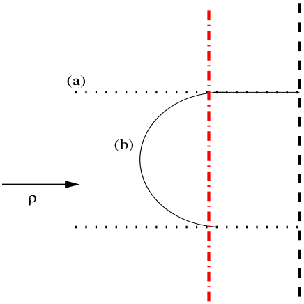
$\rho=\Lambda_{{\cal N}=1}$       $\rho=\infty$

Figure 4: Different configurations for the open string world-sheet in the evaluation of the Wilson loop. (a) corresponds to the subtraction of “two bare quarks”. (b) is the only allowed configuration (fine tuned) that leads to finite results after renormalisation, for both the potential and the quarks distance. Notice that configuration (b) hits the brane at right angles and, therefore, tends asymptotically to (a) for large $\rho$.

Before proceeding let us comment on the possible choices of this scale and its role. Admittedly, any choice seems to be arbitrary to some extent and one should wonder on a reliable value of $\Lambda$ that delimits the IR region. This in turn will have a direct impact on the uncertainty of the results. To be more definite let us remind the structure of the phases in the theory flowing from the UV to the IR region, fig. 3: in the UV region the theory is R-symmetric and the dynamics is ridden by the fields (3.8) and (3.9). In decreasing the energy the value of $\Lambda_{{\cal N}=1}$ is settled by the point $\rho^{*}$ where the gaugino starts to condensate, i.e. the R-symmetry is broken. Correspondingly the order parameter in the supergravity side is the function $a(\rho)$ in (3.1) [34] and $\Lambda_{{\cal N}=1}$ is given by the point where $a(\rho^{*})$ is sensibly different from zero. The shape of the function $a(\rho)$ is rather steep, decreasing rapidly from $a(0)=1$ to the zero value when $\rho$ increases. Indeed for $\rho\approx 5$, $a(5)\approx 10^{-3}$. Albeit we neither claim that this is the precise point nor that it has something special, we can safely say that we are already leaving the IR region and that the R-symmetry is in process of being restored. Hence $\mathcal{N}$=1 has an intrinsic scale and we shall discuss the two possible choices of the $\Lambda$ scale used in (3.14) with respect to it:

i) $\Lambda>\Lambda_{{\cal N}=1}$. This implies that the original model describes at least two different phases in the theory. This could be signaled by a discontinuity in some quantity as the Wilson loop. So far this has not been observed [21, 33].

ii) $\Lambda<\Lambda_{{\cal N}=1}$. The full theory remains in a single phase. It is known from effective field theory that in the intermediate energy range $\Lambda<E<\Lambda_{{\cal N}=1}$ there is no new threshold for massless states [35] whilst massive modes have been integrated in our case.

Therefore without any loss of generality we can identify $\Lambda\approx\Lambda_{{\cal N}=1}$ in the remainder. One should wonder of the different treatment of (3.14) in [23] and the absence of the intrinsic scale $\Lambda_{{\cal N}=1}$ in their argument. Essentially the two supergravity models are expected to be identical in the IR region, thus the difference should come from the treatment of the UV contribution. In [23] (3.14) is not splitted into two pieces. This is just as a consequence of the warp factor appearing in the conifold metric which decays extremely fast, hence catching all its contribution from the IR region. And none of the fields present in that model grows unbounded. In other words the second term in the r.h.s. of (3.14) has, if any, almost a negligible contribution. This is not the case if one insists in using only the IR metric (3.1) in the full range of $\rho$ for MN.

3.3 Glueball masses for $\mathcal{N}$=1?

As we have just discussed, albeit we can find a normalised solution for the dilaton wave function there is at least some problem in choosing the correct UV behaviour. To substantiate this point we can proceed analogously as in the QCD₃ case and obtain the associated potential. Starting from (3.12) and following the notation of (2.5) we identify the functions

$$f(\rho) = e^{2\Phi_{D}(\rho)}e^{2g(\rho)}=\frac{e^{2\Phi_{D,0}}}{2}({\rho\coth(2\rho)-\frac{\rho^{2}}{\sinh^{2}(2\rho)}-\frac{1}{4}})^{\frac{1}{2}}\sinh(2\rho)\,,$$ (3.20)

$$q(\rho) = M^{2}f(\rho)\,,\quad p(\rho)\equiv 0\,,$$

which allow to write a Schrödinger-like equation (2.6) for $\Psi=f^{1/2}\tilde{\Phi}$, with the potential (2.8) given by

Figure 5: The potential $V(\rho,M)$ for the MN model in its original variable $\rho$ (full curve) and the KS potential (dashed curve), for a value $M=\frac{4}{3}$.

$$V(\rho,M) \equiv-M^{2}+\tilde{V}(\rho)\,,$$

$$\tilde{V}(\rho) =-\frac{2\,\left(-1-20\,\rho^{2}+\left(1-4\,\rho^{2}\right)\,\cosh(4\,\rho)+32\,\rho^{3}\,\coth(2\,\rho)\right)\,{{{\rm csch}^{2}}(2\,\rho)}}{{\left(1-4\,\rho\,\coth(2\,\rho)+4\,\rho^{2}\,{{{\rm csch}^{2}}(2\,\rho)}\right)}^{2}}\,.$$

Notice that this expression is valid in the IR or in the UV region. The form of the $V(\rho,M)$ potential is rather peculiar and allows us to rewrite (2.6) in terms of the reduced potential $\tilde{V}(\rho)$ ($M$ independent) as

$$-\partial^{2}_{\rho}\Psi(\rho)+\tilde{V}(\rho)\Psi(\rho)=M^{2}\Psi(\rho)\,,$$ (3.22)

which can be interpreted as a Schrödinger equation with “energy” $M^{2}$, contrary to the QCD₃ case where the analogous equation is an eigenvalue problem only with a vanishing energy. Despite its analytic appearance, (3.3) exhibits the simple form depicted in fig. 5. (Together with it we have also displayed the potential corresponding to the KS model [18].) The potential resembles a smooth 1-dimensional step-potential in quantum mechanics, where it is well known that there are no bound states, the solutions with $E>\tilde{V}(\rho\rightarrow\infty)$ are oscillatory at infinity. The non-normalisability of the wave function solutions is reflected in the asymptotics of the potential $\tilde{V}(\rho)$, (see also fig. 5),

$$\lim_{\rho\rightarrow\infty}\tilde{V}(\rho)=1\quad{\rm and}\quad\lim_{\rho\rightarrow 0}\tilde{V}(\rho)=\frac{4}{3}\,.$$ (3.23)

It is worth noticing at this point the striking difference of shapes in fig. 5 between the Schrödinger-like potentials for the MN model and the KS model. In sharp contrast with the former, the latter can –and eventually will– exhibit a discrete spectrum of normalisable wave functions.

As we have advanced in the previous subsection, one possible way of obtaining a discrete glueball spectra is by imposing the BC (3.15) and (3.19) for the $\tilde{\Phi}$ function which correspond to

$$\Psi(0)=\Psi(\Lambda_{{\cal N}=1})=0\,,$$ (3.24)

for the $\Psi$ function . After this the potential (3.3) is supplemented with two infinite walls at $\rho=0\,,\,\Lambda_{{\cal N}=1}$. It resembles a one-dimensional infinite square well problem of width $\Lambda_{{\cal N}=1}$ and whose bottom is slightly distorted with a mean value given by the average value of (3.3), i.e., $V_{\rm{well}}=\langle\tilde{V}(\rho)\rangle$. Notice that this approach assumes that whatever sufficient smooth potential in the region $0<\rho<\Lambda_{{\cal N}=1}$ will provide similar results. In this simplified approximation, the energy levels (which correspond to the allowed values of masses squared) are given by

$$M^{2}_{n}=\left(\frac{\pi}{\Lambda_{{\cal N}=1}}\right)^{2}n^{2}+V_{\rm{well}}\,,\quad(n=1,2,\ldots)\,.$$ (3.25)

They only depend on the well width and on $V_{\rm{well}}$. Notice that for the special case of $V_{\rm{well}}=0$, the masses, normalised to the lightest one, are in the fixed ratios

$$\frac{M_{n}}{M_{1}}\approx n\,,\quad(n=1,2,\ldots)\,.$$ (3.26)

In our case $V_{\rm{well}}=\langle\tilde{V}(\rho)\rangle\simeq 1$ (see fig. 5 and (3.23)), and the mass ratios will depend on the actual value of the cut-off $\Lambda_{{\cal N}=1}$ (see below).

n	State	Lattice [12]	$\mathcal{N}$=0 [9]	$\mathcal{N}$=1 KS [23, 24]	$\mathcal{N}$=1∗ [36]
$1$	$0^{++}$	$1$	$1$	$1$	$1$
$2$	$0^{++*}$	$1.75$	$1.4$	$1.5$	$1.5$
$3$	$0^{++**}$	–	$1.9$	$2$	$1.9$
$4$	$0^{++***}$	–	$2.3$	$2.5$	–

Table 2: Glueball mass predictions of several supergravity models and the lattice computation. The ground state has been normalised to $1$ in all the cases. The lattice results are subject to errors.

It is instructive, even at this early stage, to compare these crude estimates with predictions from other models. The models considered and their corresponding results are shown in table 2, where we have normalised all masses to the lightest, corresponding to the ground state. A common feature to the models displayed in table 2 is that the glueball spectra follows approximately the relation

$$\frac{M_{n}}{M_{1}}\approx\frac{n+1}{2}\,\,(n=1,2,\ldots)\,.$$ (3.27)

The similitude between the models depicted in table 2 is not surprising. Previous calculations suggest that the ball park value of the glueball masses is almost independent of the supergravity model [16] used to calculate them. This can be understood on the basis of the WKB approximation from which it follows that the main contribution to the masses is identified by the leading contribution (the first term, r.h.s. in (2.15) in the QCD₃ case) giving already a result on the ball park of the lattice one [17] whilst the sub-leading terms in the WKB approximation (the rest of terms in r.h.s. of (2.15)) is responsible for the tiny difference between them.

The relation (3.27) is not satisfied by the infinite square well approximation with $V_{well}=0$ (3.26), indicating that the absolute normalisation of the potential and its width might play a crucial physical role. If this were not the case, our regularised MN model would not only differ in the UV region, but as a novelty also in the deep IR.

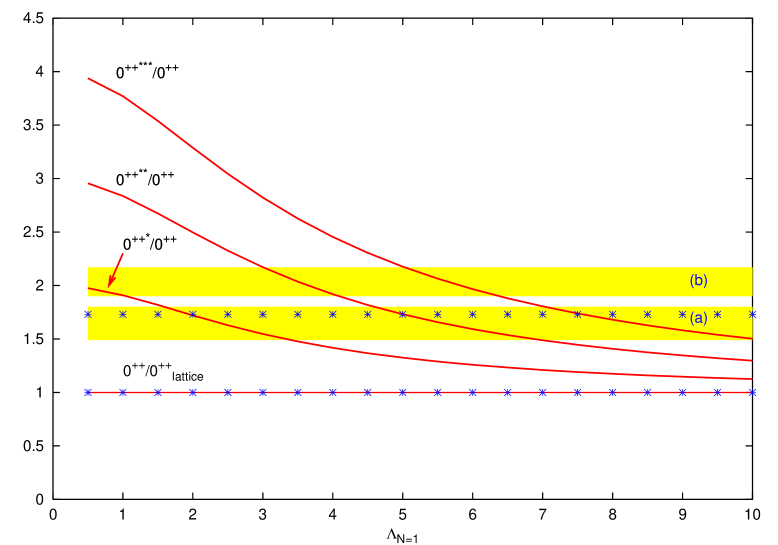
Figure 6: Predictions of glueball masses as a function of $\Lambda_{{\cal N}=1}$ (solid lines). Bands (a) and (b) correspond to edge values of $M_{0^{++*}}/M_{0^{++}}$ and $M_{0^{++**}}/M_{0^{++}}$, respectively, for the models quoted in table 2. Dots correspond to the ground and first state lattice data. The ground state has been normalised to $1$ in all the cases. The numerical uncertainties are estimated to be of the order of $2\%$.

In what follows we shall investigate further the consistency of these findings. And in order to estimate roughly the range of applicability of the model we shall compare the obtained glueball masses as a function of the $\Lambda_{{\cal N}=1}$ cut-off with the lattice predictions.

3.4 Numerology

Our numerical results have been obtained by discretising the Schrödinger equation (3.22) for the (3.3) potential with the (3.24) BC and solving for the eigenvalues using standard techniques. We collect in fig. 6 the glueball spectra (in arbitrary units) as a function of the cut-off, $\Lambda_{{\cal N}=1}$, for the first excited states. For comparison we have also depicted in the horizontal bands the range covered between the different results for the rest of the models while dots are the lattice data. As is clear, from the figure, once we push the cut-off to higher and higher-energy all the glueball masses become degenerate and tend to vanish, $M_{n}\sim n/\Lambda_{{\cal N}=1}$, thus recovering our earlier expectations of the absence of glueballs in the original model . These considerations are complementary to the arguments cited in the preceding subsection regarding the absence of discrete spectrum for solutions of the dilaton equation (3.12) covering the full range of values from $\rho=0$ to $\rho\rightarrow\infty$. Notice that the sensitivity of the glueball masses with respect to the cut-off is rather large: to use a modified cut-off accounting for the change from $\rho\approx 0.5$ to $\rho\approx 5$ drives the glueball mass of the first two excited states down by roughly $50\%$.

At this point, we are concerned that there is some degree of arbitrariness on how to fix the value of the upper bound for $\rho$, $\Lambda_{{\cal N}=1}$. Nevertheless we have just seen that for a value approximately of $\rho\approx 5$ we can safely consider that the R-symmetry has been restored and hence the theory has changed the phase. An eyeball estimate from the first excited state of fig. 6 sets, comparing to the lattice results and restoring units, $\Lambda_{{\cal N}=1}\approx 2\,l_{s}$, as the scale of the effective theory that the MN model describes. Setting this scale one obtains the following spectra normalised to $1$

$$M_{1}=1\,,\quad M_{2}\approx 1.7\,,\quad M_{3}\approx 2.5\,,\quad M_{4}\approx 3.3\,,\ldots\,,$$ (3.28)

to be compared with table 2 and with the crude estimate (3.25) using $V_{\rm well}\simeq 1$, (3.26),

$$M_{1}=1\,,\quad M_{2}\approx 1.8\,,\quad M_{3}\approx 2.6\,,\quad M_{4}\approx 3.4\,,\ldots\,.$$ (3.29)

From the same figure, obtained with the exact potential, the approximated pattern of the rest of supergravity models can be recovered for the first few states taking $\Lambda_{{\cal N}=1}\approx 3.5l_{s}$,

$$M_{1}=1\,,\quad M_{2}\approx 1.5\,,\quad M_{3}\approx 2.0\,,\quad M_{4}\approx 2.6\,,\ldots\,.$$ (3.30)

As in the QCD₃ case we can apply the WKB approximation to control the numerics. Although the approximation is valid for excited states, there is already good agreement with the exact results even for the first lowest ones differing with those by less than $5\%$.

As a last point we comment on the inclusion of non-commutative effects [33]. These are identical to the ones described in sec. 2: non-commutative effects increase the masses of the bound states. However, in this precise case the total number of glueballs remains unlimited due to the presence of the infinite walls.

We have interpreted the lack of glueball masses in the MN as an explicit way of obtaining by hand an estimate of the range of its applicability. We shall explore in the next two sections further implications of this frame.

3.5 $1^{--}$ states

We consider in what follows the linear fluctuations of the RR 2-form potential $C_{2}$. We work in the string frame and use the notation of [28] for the type–IIB supergravity. It turns out that, due to the fact that in the MN background the potentials $B_{2}$, $C_{0}$ and $C_{4}$ vanish, we can get a solution for the linearised fluctuations in this background where only the fluctuation $\tilde{C}$ of the $C_{2}$ potential is turned on. The equation of motion is

$$\partial_{\mu}\left(\sqrt{g}g^{\mu\alpha}g^{\nu\beta}g^{\rho\gamma}\partial_{[\alpha}{\tilde{C}}_{\beta\gamma]}\right)=0\,.$$ (3.31)

Assuming the simplest ansatz we take only one component (in the space directions) of the fluctuation, say $\tilde{C}_{12}$, to be different from zero. Furthermore we consider the dependencies

$$\tilde{C}_{12}=f_{12}(\rho)e^{ik\cdot x}$$ (3.32)

where $x^{\mu}$ runs over the 4-dimensional directions, $\mu=0,\dots,3\,,$ which we take Euclidean. Then we obtain

$$\frac{1}{Ng_{s}}\partial_{\rho}(e^{2\Phi_{D}(\rho)}e^{2g(\rho)}\partial_{\rho}\tilde{C}_{12})+\partial_{\mu}(e^{2\Phi_{D}(\rho)}e^{2g(\rho)}\partial_{\mu}\tilde{C}_{12})$$

$$-\partial_{1}(e^{2\Phi_{D}(\rho)}e^{2g(\rho)}\partial_{1}\tilde{C}_{12})-\partial_{2}(e^{2\Phi_{D}(\rho)}e^{2g(\rho)}\partial_{2}\tilde{C}_{12})=0\,,$$ (3.33)

together with

$$\partial_{1}\partial_{0}\tilde{C}_{12}=\partial_{1}\partial_{3}\tilde{C}_{12}=\partial_{1}\partial_{\rho}\tilde{C}_{12}=\partial_{2}\partial_{0}\tilde{C}_{12}=\partial_{2}\partial_{3}\tilde{C}_{12}=\partial_{2}\partial_{\rho}\tilde{C}_{12}=0\,.$$ (3.34)

Requiring, according to the central idea in the ansatz (3.32), that $\tilde{C}_{12}$ has a sensible $\rho$ dependence, we are led to the result $k_{1}=k_{2}=0$. Finally, we end up with

$$\partial_{\rho}\left(e^{2\Phi_{D}(\rho)}e^{2g(\rho)}\partial_{\rho}f^{\mu\nu}(\rho)\right)+M^{2}e^{2\Phi_{D}(\rho)}e^{2g(\rho)}f^{\mu\nu}(\rho)=0\,,$$ (3.35)

where $M^{2}=-(k_{0})^{2}-(k_{3})^{2}$ (with Euclidean time). This result exactly coincides with the analogous equation for the singlet dilaton fluctuations. Therefore the same conclusions obtained there hold in this case; in particular, there is no discrete spectrum of normalisable states if we look for solutions covering the full range of the transversal variable. The same way to fix this problem as in the case of the dilaton can be used here, and so we end up with a degenerate spectrum for the dilaton fluctuations and the RR 2-form fluctuations.

3.6 Kaluza–Klein modes of $S^{2}$

The scenario presented in [21] possesses many of the desired features one would like to find in QCD-like theories as chiral symmetry breaking and the correct $\beta$-function that matches precisely the one obtained from $\mathcal{N}$=1 SYM field theory. In addition, in order to deal with a well-defined low-energy effective theory, it is also desirable that the theory contains a mass gap between the singlet (physical) and non-singlet states, being the latter heavier enough to decouple. By themselves, their spectrum can be either continuum or discrete. It is also well known that qualitative arguments indicate some contamination from spurious non-singlet states obtained after the reduction of the $S^{2}$ that should properly have decoupled in the IR

$$M^{2}_{\rm{glueballs}}\sim M^{2}_{\rm{KK}}\sim\frac{1}{Ng_{s}\alpha^{\prime}}\,,$$

and as a consequence they do not decouple in the limit of the validity of the supergravity description, that requires $Ng_{s}\gg 1$. Nevertheless, there is evidence [37] that going beyond the supergravity approximation (in the sense of introducing string solitons), the analogue stringy KK modes on the $S^{2}$ sphere indeed decouple for large values of the R-charge. We shall in the remainder analyse the fate of the supergravity (point-like) KK modes in more detail and check whether the decoupling observed for the stringy KK modes still holds.

We use the complete ansatz (3.11) for the fluctuations of the dilaton with modes on the $S^{2}$. As a matter of fact, one does not need to consider modes on the $S^{3}$ because the 3-cycle appears when we uplift our solution of 7-dimensional supergravity to 10 dimensions. Taking into account the truncation from type–IIB to the 7-dimensional supergravity, this means that we can have solutions for the fluctuations starting from the 7-dimensional solution and then uplifting it: no fluctuation modes will be turned on the $S^{3}$ if we do not perform further transformations on the solutions.

The inclusion in the present ansatz of dependencies on the variables of the $S^{2}$ makes it necessary to compute the components $g^{\theta\theta}$ and $g^{\varphi\varphi}$ of the metric. It turns out that these components are not affected by the presence of the gauge fields $A^{a}$ in (3.1). The equation of motion for the non-singlet states reads

$$\partial_{\rho}(e^{2\Phi_{D}(\rho)}e^{2g(\rho)}\partial_{\rho}\tilde{\Phi})+\left(e^{2\Phi_{D}(\rho)}e^{2g(\rho)}N\alpha^{\prime}g_{s}M^{2}-l(l+1)e^{2\Phi_{D}(\rho)}\right)\tilde{\Phi}=0\,,$$ (3.36)

and one can already observe that the sign of the angular momentum contribution is opposite to the $M^{2}$ one, in a similar way as in section (2.1). The potential obtained from (3.36) has a centrifugal barrier similar as in 3-dimensional central potentials,

$$V(\rho,M,l)={\rm eq}.~{}(\ref{MNpot-original})+8l(l+1)\frac{\sinh^{2}(2\rho)}{1-8\rho^{2}-\cosh(4\rho)+4\rho\sinh(4\rho)}\,.$$

The term with the angular momentum dependence behaves as $\sim 1/\rho^{2}$ for $\rho\rightarrow 0$ and tends to zero for large $\rho$. It is again obvious that the shape of this potential, steadily falling from infinity at $\rho=0$ to the asymptotic value $1-M^{2}$ at $\rho\rightarrow\infty$, will prevent the model from exhibiting a discrete spectrum of normalisable wave functions. We can still adopt the same drastic procedure of imposing a hard cut-off, as we did for the glueballs. Since the potential is sensitive to the singularity only very close to the origin, one expects that the mass spectrum for the first excited states being of the same order of magnitude as for the glueballs spectrum. We have verified this claim numerically. Indeed, the KK masses for $l=1$, using $\Lambda_{{\cal N}=1}=2$ and normalising to the singlet $0^{++}$ ground state, are

$$M_{1}\approx 2.4\,,\quad M_{2}\approx 3.7\,,\quad M_{3}\approx 5.1\,,\quad M_{4}\approx 6.5\,,\ldots\,.$$ (3.37)

We conclude that, within this interpretation of the model, which allows for the introduction of the hard cut-off at the scale of the R-symmetry breaking, there is no decoupling of the KK supergravity modes.

4 Summary and discussion

Extending the AdS/CFT correspondence to non-supersymmetric and/or non-maximally supersymmetric theories we have computed the glueball spectrum for the non-commutative QCD₃ and for $\mathcal{N}$=1 SYM Maldacena–Núñez model. We have assumed that the same relation as in AdS/CFT holds in these cases, and thus we have identified the glueball spectrum with the one coming from the dilaton in type–IIB strings.

In the case of QCD₃ the inclusion of a non-commutative parameter, $\theta$, does not improve the lack of decoupling of the non-singlets KK states with respect to the singlet ones. As a general feature of this model we see that the potential reaches its minimum at $\theta=0$. For $\theta\neq 0$ the parameter plays the same role as the strength of the electric potential in a cool emission of electrons from a metal: in increasing $\theta$ the number of bound states decreases. It exists a critical value of $\theta$ where there is no longer any bound state in the system, see fig. 1.

The most relevant findings are concerning the glueball spectra of the MN model. To obtain the spectra we looked at the poles of massless dilaton two-point function: in order to get any n-point Green function one shall simply take n-functional derivatives on the generating functional defined in (1.1) considering the fields $\phi$ as external sources for the operators ${\cal O}$. For the two-point Green-function in momentum-space case this gives

$$\big{\langle}{\cal O}_{4}(l){\cal O}_{4}(m)\big{\rangle}=\frac{\partial^{2}S[\phi]}{\partial\phi_{l}\partial\phi_{m}}\,.$$ (4.1)

Taking the minimal massless action for the fluctuations of the scalar field in the IR region of the MN background (in the string frame)

$$S=\frac{1}{4\kappa_{10}^{2}}\int d^{10}\,x\,e^{3\Phi_{D}(\rho)}e^{2g(\rho)}g^{\mu\nu}\partial_{\mu}\phi\partial_{\nu}\phi$$ (4.2)

with all the rest of fields set to zero and integrating by parts, one can identify easily the dilaton e.o.m. (3.12) with $M=0$. If we further set to zero all the boundary terms coming from the $\mathbb{R}^{4}$ integration the action takes the form

$$S=\frac{1}{16\kappa_{10}^{2}}\left(\frac{N}{4}\right)^{3/2}\int_{S^{3}}d\Omega_{3}^{2}\int_{S^{2}}d\Omega_{2}^{2}\int_{0}^{\Lambda_{{\cal N}=1}}d^{4}\,x\left({\cal F}(x^{\mu},\rho)-{\cal F}(x^{\mu},0)\right)\,,$$ (4.3)

where we have defined the flux factor ${\cal F}(x^{\mu},\rho)\equiv e^{3\Phi_{D}(\rho)}e^{2g(\rho)}\phi(x^{\mu},\rho)\,\partial_{\rho}\phi(x^{\mu},\rho)$. Notice that even at this earlier stage one can realise that the previous flux factor can not be extended to the full range of $\rho$ if its value has to be bounded, signaling that we have to change to the S-dual version of the metric.

In order to find a discrete spectrum for normalisable glueball states we have first considered the problem of the runaway of the dilaton. Since this causes the supergravity approximation to lose its validity, we are led to move at some moment to the S-dual solution. This means that we shall use (3.1) in the IR region together with the BC $\Psi(0)=0$ and (3.8) with the BC $\Psi(\rho\rightarrow\infty)=0$ at the UV. Notice that there is an intermediate region where both descriptions fail to give a reliable description, shadow area in fig. 3. The equation for the fluctuations for the dilaton remains the same in both regions and the only change is in the definition of the norm of our wave function. It turns out that all solutions become normalisable and consequently there is no discrete spectrum. This conclusion is in flat disagreement with the findings through the Wilson loop [21]. To disentangle this puzzle we noticed that: i) the expectation that the existence of an area law in the Wilson loop, as defined by [31, 32], does not necessary implies the existence of the glueball spectra in our case. This is probably not only due to the non-conformal nature of the model but as a consequence of the dilaton blowing up at the UV region. ii) One can amend the model by setting by hand a hard cut-off identified with the R-symmetry scale, $\Lambda_{{\cal N}=1}$. Above the cut-off the model makes no sense whilst below can be interpreted as an effective description of $\mathcal{N}$=1 SYM. In doing so we enforce the existence of the spectra with a distribution rather similar to the one of a square-well potential in quantum mechanics. This can be justified to a considerable extent, on the basis of the R-symmetry breaking of the underlying field theory. Within this regularisation and relying on the lattice values of the two lightest $0^{++}$ states, we have set the scale of applicability of the model, $\Lambda_{{\cal N}=1}\approx 2\,l_{s}$. The lack of lattice results for higher excitations prevents us from checking the consistency of these results. As a consequence of this choice, notice that the MN model does not only differ from similar models (KS, $\mathcal{N}$=1^∗) in the UV region as mentioned earlier in the literature but also in the IR. We should point out that, while the glueball spectra in the rest of supergravity models are in reasonable agreement among themselves, the MN one clearly does not follow this general trend. Otherwise, we can recover a pattern similar to the rest of supergravity models discarding the previous value of $\Lambda_{{\cal N}=1}$. In this case a value $\Lambda_{{\cal N}=1}\approx 3.5\,l_{s},$ is favoured.

Using the same approach, and to test further its implications, we have computed the $1^{--}$ states spectra. It turns out that it reduces to the RR 2-form $C_{2}$ and is degenerate with $0^{++}$.

We have also studied the KK modes appearing on the $S^{2}$. Like in the previous two cases there is need for regularisation. After this, it is unlikely that the model presents decoupling.

All in all, we point out that the MN model does not display a discrete glueball spectra by itself. With a rude regularisation we interpret it as a low-energy effective theory and estimate its range of validity, that turns out to be quite limited. Even though we do not claim that the amended model is ruled out, it is hard to believe that it gives any sensible results, unless one finds a precise determination, coming from the model alone –or some improvement of it–, of the value of the cut-off $\Lambda_{{\cal N}=1}$.

Acknowledgements

We are grateful to Rafael Hernández and Carlos Núñez for useful discussions and comments. This work is partially supported by MCYT FPA, 2001-3598, CIRIT, GC 2001SGR-00065, and HPRN-CT-2000-00131. J.M.P. acknowledges the Spanish ministry of education for a grant.

Appendix A Schwarzian derivative and reparameterisation

Aiming at the determination of the spectrum of masses $M$, it is convenient to write the equation as a zero-energy one-dimensional quantum mechanical problem,

$$\frac{d^{2}\psi}{du^{2}}-V(u)\psi=0\,,$$ (A.1)

where the potential $V(u)$ already carries the parameter $M$ whose spectrum we are looking for.

To bring a general equation of the type,

$$\partial_{u}(f(u)\partial_{u}\phi)+g(u)\phi=0\,,$$ (A.2)

to the form (A.1) we use a multiplicative factor for $\phi$ to define a new function $\psi:=(f(u))^{\frac{1}{2}}\phi$. The potential obtained has already been written in (2.8), with $g(u)=M^{2}h(u)+p(u)$.

Notice that we still have to our avail the freedom of reparameterisation, that is, of changing the coordinate system, $u\rightarrow\omega,\,u=F(\omega)$. This change will bring an equation of the type (A.1) again to the general form (A.2), but a new multiplicative factor will transform the equation into the Schrödinger form, with a new potential $\tilde{V}(\omega)$. A simple computation shows that the new potential is related to the old one by

$$\tilde{V}(\omega)=V(F(\omega))(\partial_{\omega}F)^{2}-\frac{1}{2}Q_{F}(\omega)\,,$$ (A.3)

where

$$Q_{F}(\omega):=\left(\frac{F^{\prime\prime}}{F^{\prime}}\right)^{\prime}-\frac{1}{2}\left(\frac{F^{\prime\prime}}{F^{\prime}}\right)^{2}$$ (A.4)

is the Schwarzian derivative of $F$ ($F^{\prime}$ stands for $\partial_{w}F$).

The reason for the appearance of the Schwarzian derivative becomes clear when one takes into account that composition of two reparameterisations is a closed operation resulting in a third one and that, under such a composition, the Schwarzian derivative satisfies the key property

$$Q_{F\circ G}(\omega)=Q_{F}(G(\omega))\,(G^{\prime}(\omega))^{2}+Q_{G}(\omega)\,.$$ (A.5)

Indeed, under an infinitesimal coordinate transformation $u\rightarrow u-\epsilon(u)$, the potential transforms as

$$\delta V=\epsilon V^{\prime}+2\epsilon^{\prime}V-\frac{1}{2}\epsilon^{\prime\prime\prime}\,,$$ (A.6)

which is the standard transformation rule for a weight 2 scalar density under reparameterisations with an additional “anomalous” term $\epsilon^{\prime\prime\prime}$, which is compatible with the algebra of reparameterisations. Notice that the coefficient in front of this term can be arbitrarily varied by just redefining $V$ in (A.6) with a numerical factor. With $\frac{c}{12}$ instead of $-\frac{1}{2}$, (A.6) matches the transformation rule for the energy-momentum tensor of two-dimensional quantum conformal field theories, where $c$ is the conformal anomaly.

The result (A.3) provides us therefore with an indirect method to integrate the infinitesimal transformation (A.6). A direct method, which essentially exponentiates the function $\epsilon$, can be found in [38].

Appendix B On the WKB method and reparameterisation

Let us make a comment on the WKB method, when applied to the determination of the energy spectrum of bound states. Suppose we are given a Schrödinger equation with a potential ${\cal V}$ suitable for the application of the method, with two turning points, $x_{1},\,x_{2}$, for the equation $E-{\cal V}(x)=0$ in a certain interval of values of the energy $E$. The WKB formula for the spectrum of energies is

$$I(n)\equiv\left(n+\frac{1}{2}\right)\pi=\int_{x_{1}}^{x_{2}}dx\sqrt{E-{\cal V}(x)}\,,\quad n=0,\,1,\,2,\,\dots\,.$$ (B.7)

Now let us introduce an infinitesimal reparameterisation , $x\rightarrow x+\epsilon(x)$. One can compute, to first order in $\epsilon$, the new potential for the new Schrödinger-like equation. Since the transformation is infinitesimal, it is still an eigenvalue problem, the new potential being ${\cal\tilde{V}}={\cal V}+\delta{\cal V}$, with $\delta{\cal V}$ as in (A.6). Accordingly, the turning points undergo a change,

$$x_{0,1}\rightarrow{\tilde{x}}_{i}=x_{i}-\epsilon(x_{i})+\frac{1}{2}\frac{\epsilon^{\prime\prime\prime}(x_{i})}{{\cal V}^{\prime}}\,,$$ (B.8)

whereas the new expression for (B.7) becomes

$$I(n)\equiv\left(n+\frac{1}{2}\right)\pi = \int_{{\tilde{x}}_{1}}^{{\tilde{x}}_{2}}dx\sqrt{E-{\cal\tilde{V}}(x)}$$

$$= \int_{x_{1}}^{x_{2}}dx\sqrt{E-{\cal V}(x)}+\frac{1}{4}\int_{x_{1}}^{x_{2}}dx\frac{\epsilon^{\prime\prime\prime}(x)}{\sqrt{E-{\cal V}(x)}}\,,\quad n=0,\,1,\,2,\,\dots\,.$$

We have the previous expression but with a new contribution to the r.h.s. Here we see in this last term an unwanted correction to the WKB formula, originated from the Schwarzian derivative term. Should the WKB formula be an exact one no matter the coordinate system, this last term would not exist. But this correction is unavoidable for general reparameterisations and in a certain sense reflects the fact that the WKB formula is only approximate. For instance, in the particular case where it gives the exact result for the spectrum when using, say, the $x$ coordinates, the spectrum will no longer be the exact one when using the new coordinates ${\tilde{x}}$. At first sight this might seem strange, even dangerous, as a paradox built in the WKB method, but it is just an outcome of its approximate nature. Notice, however, the important point one can deduce from (B): for energies $E$ sufficiently large, this correction term becomes negligible. This valuable result is in the line of the usual assertion that for large quantum numbers the errors given by the WKB method are small. We think that this argument can be extended, by iterations of the infinitesimal transformation, to general reparameterisations that yield potentials still suitable for the application of the WKB method, and that the correction term to the WKB formula due to the Schwarzian derivative will always be sub-leading with respect to the main term.

Appendix C Normalisation for the Schödinger wave function

In our procedure to deal with equation (2.6) through WKB methods, we have reformulated and converted it into a Schrödinger-like equation. It is therefore necessary to discuss the normalisation of the corresponding wave function. To this end we must first write down the normalisation associated with (1.2). The requirement of hermiticity of the Laplace operator induces the natural normalisation, in the Einstein frame,

$$\int d\rho\sqrt{g}|\Phi|^{2}\,.$$ (C.10)

Now consider the steps taken to bring equation(2.5) to a Schrödinger-like form, with $f=\sqrt{g}g^{\rho\rho}$ and $\Psi=f^{1/2}\Phi$ ,

$$\int d\rho\,\sqrt{g}|\Phi|^{2}=\int d\rho\,\sqrt{g}f^{-1}|\Psi|^{2}=\int d\rho\,g_{\rho\rho}|\Psi|^{2}\,.$$ (C.11)

This last expression is the normalisation we were seeking for. Under the reparameterisation $\rho=F(\omega)$, and with $\tilde{A}$ representing the transformed of a generic object $A$, the only component $g_{\rho\rho}$ of the one-dimensional metric $g_{\rho\rho}d\rho^{2}$ behaves as a weight=2 scalar density, $\tilde{g}_{\omega\omega}=g_{\rho\rho}(F^{\prime})^{2}$, whereas the wave function $\Psi$ behaves as a weight=(-1/2) scalar density, $\tilde{\Psi}=\Psi(F^{\prime})^{-1/2}$, thus producing the invariance

$$\int d\rho\,g_{\rho\rho}|\Psi|^{2}=\int d\omega\,\tilde{g}_{\omega\omega}|\tilde{\Psi}|^{2}\,.$$ (C.12)

We conclude that our one-dimensional Schrödinger problem includes two pieces of information, the Schrödinger-like equation itself, (A.1), and a one-dimensional metric, $g_{\rho\rho}d\rho^{2}$, originated in (1.2) that plays a role in the definition of the wave function normalisation.

References

- [1] J. M. Maldacena, “The large limit of superconformal field theories and supergravity,” Adv. Theor. Math. Phys. 2 (1998) 231 [Int. J. Theor. Phys. 38 (1999) 1113] [arXiv:hep-th/9711200];
- [2] S. S. Gubser, I. R. Klebanov and A. M. Polyakov, “Gauge theory correlators from non-critical string theory,” Phys. Lett. B 428 (1998) 105 [arXiv:hep-th/9802109];
- [3] E. Witten, “Anti-de Sitter space and holography,” Adv. Theor. Math. Phys. 2 (1998) 253 [arXiv:hep-th/9802150].
- [4] A. Kehagias and K. Sfetsos, “On running couplings in gauge theories from type-IIB supergravity,” Phys. Lett. B 454 (1999) 270 [arXiv:hep-th/9902125].
- [5] E. Witten, “Anti-de Sitter space, thermal phase transition, and confinement in gauge theories,” Adv. Theor. Math. Phys. 2 (1998) 505 [arXiv:hep-th/9803131].
- [6] G. T. Horowitz and H. Ooguri, “Spectrum of large N gauge theory from supergravity,” Phys. Rev. Lett. 80 (1998) 4116 [arXiv:hep-th/9802116].
- [7] D. J. Gross and H. Ooguri, “Aspects of large N gauge theory dynamics as seen by string theory,” Phys. Rev. D 58 (1998) 106002 [arXiv:hep-th/9805129].
- [8] A. Hashimoto and Y. Oz, “Aspects of QCD dynamics from string theory,” Nucl. Phys. B 548 (1999) 167 [arXiv:hep-th/9809106].
- [9] C. Csaki, H. Ooguri, Y. Oz and J. Terning, “Glueball mass spectrum from supergravity,” JHEP 9901 (1999) 017 [arXiv:hep-th/9806021].
- [10] R. de Mello Koch, A. Jevicki, M. Mihailescu and J. P. Nunes, “Evaluation of glueball masses from supergravity,” Phys. Rev. D 58 (1998) 105009 [arXiv:hep-th/9806125].
- [11] M. Zyskin, “A note on the glueball mass spectrum,” Phys. Lett. B 439 (1998) 373 [arXiv:hep-th/9806128].
- [12] C. J. Morningstar and M. J. Peardon, “Efficient glueball simulations on anisotropic lattices,” Phys. Rev. D 56 (1997) 4043 [arXiv:hep-lat/9704011]; C. J. Morningstar and M. J. Peardon, “The glueball spectrum from an anisotropic lattice study,” Phys. Rev. D 60 (1999) 034509 [arXiv:hep-lat/9901004].
- [13] H. Ooguri, H. Robins and J. Tannenhauser, “Glueballs and their Kaluza-Klein cousins,” Phys. Lett. B 437 (1998) 77 [arXiv:hep-th/9806171].
- [14] J. G. Russo, “New compactifications of supergravities and large N QCD,” Nucl. Phys. B 543 (1999) 183 [arXiv:hep-th/9808117].
- [15] C. Csaki, Y. Oz, J. Russo and J. Terning, “Large N QCD from rotating branes,” Phys. Rev. D 59 (1999) 065012 [arXiv:hep-th/9810186].
- [16] J. A. Minahan, “Glueball mass spectra and other issues for supergravity duals of QCD models,” JHEP 9901 (1999) 020 [arXiv:hep-th/9811156].
- [17] C. Csaki, J. Russo, K. Sfetsos and J. Terning, “Supergravity models for 3+1 dimensional QCD,” Phys. Rev. D 60 (1999) 044001 [arXiv:hep-th/9902067].
- [18] I. R. Klebanov and M. J. Strassler, “Supergravity and a confining gauge theory: Duality cascades and chiSB-resolution of naked singularities,” JHEP 0008 (2000) 052 [arXiv:hep-th/0007191].
- [19] I. R. Klebanov and E. Witten, “Superconformal field theory on threebranes at a Calabi–Yau singularity,” Nucl. Phys. B 536 (1998) 199 [arXiv:hep-th/9807080].
- [20] I. R. Klebanov and A. A. Tseytlin, “Gravity duals of supersymmetric SU(N) x SU(N+M) gauge theories,” Nucl. Phys. B 578 (2000) 123 [arXiv:hep-th/0002159].
- [21] J. M. Maldacena and C. Nunez, “Towards the large N limit of pure N = 1 super Yang Mills,” Phys. Rev. Lett. 86 (2001) 588 [arXiv:hep-th/0008001].
- [22] A. H. Chamseddine and M. S. Volkov, “Non-Abelian BPS monopoles in N = 4 gauged supergravity,” Phys. Rev. Lett. 79 (1997) 3343 [arXiv:hep-th/9707176].
- [23] E. Caceres and R. Hernandez, “Glueball masses for the deformed conifold theory,” Phys. Lett. B 504 (2001) 64 [arXiv:hep-th/0011204].
- [24] M. Krasnitz, “A two point function in a cascading N = 1 gauge theory from supergravity,” arXiv:hep-th/0011179.
- [25] J. M. Maldacena and J. G. Russo, “Large N limit of non-commutative gauge theories,” JHEP 9909 (1999) 025 [arXiv:hep-th/9908134].
- [26] J. G. Russo and K. Sfetsos, “Rotating D3 branes and QCD in three dimensions,” Adv. Theor. Math. Phys. 3 (1999) 131 [arXiv:hep-th/9901056].
- [27] M. Bertolini and P. Merlatti, “A note on the dual of N = 1 super Yang-Mills theory,” Phys. Lett. B 556 (2003) 80 [arXiv:hep-th/0211142].
- [28] J. Polchinski, “String Theory. Vol. 2: Superstring Theory And Beyond,” Cambridge University Press (2000).
- [29] J. H. Schwarz, “Covariant Field Equations Of Chiral N=2 D = 10 Supergravity,” Nucl. Phys. B 226 (1983) 269.
- [30] H. J. Kim, L. J. Romans and P. van Nieuwenhuizen, “The Mass Spectrum Of Chiral N=2 D = 10 Supergravity On S**5,” Phys. Rev. D 32 (1985) 389.
- [31] S. J. Rey and J. Yee, “Macroscopic strings as heavy quarks in large N gauge theory and anti-de Sitter supergravity,” Eur. Phys. J. C 22 (2001) 379 [arXiv:hep-th/9803001].
- [32] J. M. Maldacena, “Wilson loops in large N field theories,” Phys. Rev. Lett. 80 (1998) 4859 [arXiv:hep-th/9803002].
- [33] T. Mateos, J. M. Pons and P. Talavera, “Supergravity dual of noncommutative N = 1 SYM,” Nucl. Phys. B 651 (2003) 291 [arXiv:hep-th/0209150].
- [34] R. Apreda, F. Bigazzi, A. L. Cotrone, M. Petrini and A. Zaffaroni, “Some comments on N = 1 gauge theories from wrapped branes,” Phys. Lett. B 536 (2002) 161 [arXiv:hep-th/0112236].
- [35] T. Appelquist and J. Terning, “On the limits of chiral perturbation theory,” Phys. Rev. D 47 (1993) 3075 [arXiv:hep-ph/9211223].
- [36] D. E. Crooks and N. Evans, “The Yang Mills* Gravity Dual,” arXiv:hep-th/0302098.
- [37] J. M. Pons and P. Talavera, “Semi-classical string solutions for N = 1 SYM,” arXiv:hep-th/0301178.
- [38] X. Gracia, J. M. Pons and J. Roca, “Closure of reparametrization algebras and flow dependence of finite reparametrizations,” Int. J. Mod. Phys. A 9 (1994) 5001.
- [39] S. C. Miller and R. J. Good, “A WKB-Type Approximation to the Schrödinger Equation,” Phys. Rev. 91 (1953) 174.