Branes, Calibrations and Supergravity

Abstract.

These notes are based on lectures given at the Clay School on Geometry and String Theory, Isaac Newton Institute, Cambridge, 25 March - 19 April 2002. They attempt to provide an elementary and somewhat self contained discussion of the construction of supergravity solutions describing branes wrapping calibrated cycles, emphasising the geometrical aspects and focusing on D=11 supergravity. Following a discussion of the role of special holonomy backgrounds in D=11 supergravity, the basic membrane and fivebrane solutions are reviewed and the connection with the AdS/CFT correspondence is made. The world-volume description of branes is introduced and used to argue that branes wrapping calibrated cycles in special holonomy manifolds preserve supersymmetry. The corresponding supergravity solutions are constructed first in an auxiliary gauged supergravity theory which is obtained via Kaluza-Klein reduction.

1. Introduction

Supergravity theories in D=10 and D=11 spacetime dimensions play an important role in string/M-theory since they describe the low-energy dynamics. There are five different string theories all in D=10. At low energies the type IIA and type IIB string theories give rise to type IIA and type IIB supergravity, respectively, while the type I, and the two heterotic string theories all give rise to type I supergravities. The five string theories are all related to each other, possibly after compactification, by various dualities. There are also dualities which relate string theory to M-theory, which resides in D=11. M-theory is much less understood than string theory, but one of the most important things that is known about it, is that its low-energy effective action is given by D=11 supergravity.

Solutions to the supergravity equations of motion, particularly those that preserve some supersymmetry, are of interest for many reasons. One reason is that they are useful in studying compactifications from D=10 or 11 down to a lower dimensional spacetime. By compactifying down to four spacetime dimensions, for example, one might hope to make contact with particle physics phenomenology. In addition to strings, it is known that string theory has a rich spectrum of other extended objects or “branes”. Indeed supergravity solutions can be constructed describing the geometries around such branes, and these provide a very important description of the branes. Similarly, there are membrane and fivebrane solutions of D=11 supergravity, which will be reviewed later, which implies that M-theory contains such branes. An important application of brane and more general intersecting brane solutions is that they can be used to effectively study the quantum properties of black holes.

Supergravity solutions also provide powerful tools to study quantum field theories. The most significant example is Maldacena’s celebrated AdS/CFT correspondence [108] which conjectures that string/M-theory on certain supergravity geometries that include anti-de-Sitter (AdS) space factors, is equivalent to certain conformally invariant quantum field theories (CFTs). The supergravity approximation to string/M-theory allows one to calculate highly non-trivial information about the conformal field theories.

The AdS/CFT correspondence is truly remarkable. On the one hand it states that certain quantum field theories, that a priori have nothing to do with gravity, are actually described by theories of quantum gravity (string/M-theory). Similarly, and equally surprising, it also states that quantum gravity on certain geometries, is actually quantum field theory. As a consequence much effort has been devoted to further understanding and generalising the correspondence.

The basic AdS/CFT examples arise from studying the supergravity solutions describing planar branes in flat space, in the “near horizon limit”. Roughly speaking, this is the limit close to the location of the brane. Here we shall discuss more general supergravity solutions that describe branes that are partially wrapped on various calibrated cycles within special holonomy manifolds. We will construct explicit solutions in the near horizon limit, which is sufficient for applications to the AdS/CFT correspondence.

To keep the presentation simple, we will mostly restrict our discussion to D=11 supergravity. In an attempt to make the lectures accessible to both maths and physics students we will emphasise the geometrical aspects and de-emphasise the quantum field theory aspects. To make the discussion somewhat self contained, we begin with some basic material; it is hoped that the discussion is not too pedestrian for the physics student and not too vague for the maths student!

We start with an introduction to D=11 supergravity, defining the notion of a bosonic solution of D=11 supergravity that preserves supersymmetry. We then describe why manifolds with covariantly constant spinors, and hence with special holonomy, are important. Following this we present the geometries describing planar membranes and fivebranes. These geometries have horizons, and in the near horizon limit we obtain geometries that are products of $AdS$ spaces with spheres, which leads to a discussion of the basic AdS/CFT examples.

To motivate the search for new AdS/CFT examples we first introduce the world-volume description of branes. Essentially, this is an approximation that treats the branes as “probes” propagating in a fixed background geometry. We define calibrations and calibrated cycles, and explain why such probe-branes wrapping calibrated cycles in special holonomy manifolds preserve supersymmetry. The aim is then to construct supergravity solutions describing such wrapped branes after including the back-reaction of the branes on the special holonomy geometry.

The construction of these supergravity solutions is a little subtle. In particular, the solutions are first constructed in an auxiliary gauged supergravity theory. We will focus, for illustration, on the geometries corresponding to wrapped fivebranes. For this case the solutions are first found in $SO(5)$ gauged supergravity in D=7. This theory arises from the consistent truncation of the dimensional reduction of D=11 supergravity on a four-sphere, as we shall discuss. This means that any solution of the D=7 supergravity theory automatically gives a solution of D=11 supergravity. We will present several details of the construction of the solutions describing fivebranes wrapping SLAG 3-cycles, and summarise more briefly the other cases. We also comment on some aspects of the construction of the solutions for wrapped membranes and D3-branes of type IIB supergravity.

We conclude with a discussion section that outlines some open problems as well as a brief discussion of other related work on the construction of wrapped NS-fivebranes of type IIB supergravity.

2. D=11 supergravity

The bosonic field content of D=11 supergravity [36] consists of a metric, $g$, and a three-form $C$ with four-form field strength $G=dC$ which live on a D=11 manifold which we take to be spin. The signature is taken to be mostly plus, $(-,+,\dots,+)$. In addition the theory has a fermionic gravitino, $\psi_{\mu}$. The action with $\psi_{\mu}=0$ is given by

(2.1) $$S=\frac{1}{2\kappa^{2}}\int d^{11}x{\sqrt{-g}}R-\frac{1}{2}G\wedge*G-\frac{1}{6}C\wedge G\wedge G~{},$$

and thus the bosonic equations of motion, including the Bianchi identity for the four-form, are

$$R_{\mu\nu} = \frac{1}{12}(G^{2}_{\mu\nu}-\frac{1}{12}g_{\mu\nu}G^{2})$$

$$d*G+\frac{1}{2}G\wedge G = 0$$

(2.2) $$dG = 0~{},$$

where $G^{2}_{\mu\nu}=G_{\mu\sigma_{1}\sigma_{2}\sigma_{3}}G{{}_{\nu}}{{}^{\sigma_{1}\sigma_{2}\sigma_{3}}}$ and $G^{2}=G_{\sigma_{1}\sigma_{2}\sigma_{3}\sigma_{4}}G^{\sigma_{1}\sigma_{2}\sigma_{3}\sigma_{4}}$, with $\mu,\nu,\sigma=0,1,\dots,10$. The theory is invariant under supersymmetry transformations whose infinitesimal form is given schematically by

$$\delta g \sim \epsilon\psi$$

$$\delta C \sim \epsilon\psi$$

(2.3) $$\delta\psi \sim \hat{\nabla}\epsilon+\epsilon\psi\psi~{},$$

where the spinor $\epsilon$ parametrises the variation and the connection $\hat{\nabla}$ will be given shortly.

Of primary interest are bosonic solutions to the equations of motion that preserve at least one supersymmetry. These are solutions to the equations of motion with $\psi=0$ which are left inert under a supersymmetry variation. From (2) we see that $\delta g=\delta C=0$ trivially, and hence we seek solutions to the equations of motion that admit non-trivial solutions to the equation $\hat{\nabla}\epsilon=0$.

As somewhat of an aside we mention a potentially confusing point. For the theory to be supersymmetric, it is necessary that all of the fermions are Grasssmann odd (anti-commuting) spinors. However, since the only place that fermions enter into bosonic supersymmetric solutions is via $\hat{\nabla}\epsilon=0$ and since this is linear in $\epsilon$ we can, and will, take $\epsilon$ to be a commuting (i.e. ordinary) spinor from now on. The Grassmann odd character of the fermions is certainly important in the quantum theory, but this will not concern us here.

To be more precise about the connection $\hat{\nabla}$ let us introduce some further notation. We will use the convention that $\mu,\nu,\dots$ are co-ordinate indices and $\alpha,\beta,\dots$ are tangent space indices, i.e., indices with respect to an orthonormal frame. The D=11 Clifford algebra, $Cliff(10,1)$, is generated by gamma-matrices $\Gamma^{\alpha}$ satisfying the algebra

(2.4) $$\Gamma^{\alpha}\Gamma^{\beta}+\Gamma^{\alpha}\Gamma^{\beta}=2\eta^{\alpha\beta}~{},$$

with $\eta=diag(-1,1,\dots,1)$. We will work in a representation where the gamma-matrices are real $32\times 32$ matrices acting on real 32 component spinors, with $\Gamma_{0}\Gamma_{1}\dots\Gamma_{10}=+1$. Recall that $Spin(10,1)$ is generated by

(2.5) $$\frac{1}{4}\Gamma^{\alpha\beta}\equiv\frac{1}{8}\left(\Gamma^{\alpha}\Gamma^{\beta}-\Gamma^{\alpha}\Gamma^{\beta}\right)~{},$$

and here we have introduced the notation that $\Gamma^{\alpha_{1}\dots\alpha_{p}}$ is an anti-symmetrised product of $p$ gamma-matrices. The charge conjugation matrix is defined to be $\Gamma_{0}$ and $\bar{\epsilon}\equiv\epsilon^{\mathrm{T}}\Gamma_{0}$.

We can now write the condition for a bosonic configuration to preserve supersymmetry as

(2.6) $$\hat{\nabla}_{\mu}\epsilon\equiv\nabla_{\mu}\epsilon+\frac{1}{288}[\Gamma{{}_{\mu}}{{}^{\nu_{1}\nu_{2}\nu_{3}\nu_{4}}}-8\delta{{}_{\mu}^{\nu_{1}}}\Gamma^{\nu_{2}\nu_{3}\nu_{4}}]G_{\nu_{1}\nu_{2}\nu_{3}\nu_{4}}\epsilon=0~{},$$

where $\nabla_{\mu}\epsilon$ is the usual covariant derivative on the spin bundle

(2.7) $$\nabla_{\mu}\epsilon=(\partial_{\mu}+\frac{1}{4}\omega_{\mu\alpha\beta}\Gamma^{\alpha\beta})\epsilon~{}.$$

Observe that the terms involving the four-form in (2.6) imply that $\hat{\nabla}$ takes values in the Clifford algebra and not just the Spin subalgebra. This is the typical situation in supergravity theories but there are exceptions, such as type I supergravity, where the connection takes values in the spin subalgebra and has totally anti-symmetric torsion [135].

Non-trivial solutions to (2.6) are called Killing spinors. The nomenclature is appropriate since if $\epsilon^{i}$, $\epsilon^{j}$ are Killing spinors then $K^{ij\mu}\equiv\bar{\epsilon}^{i}\Gamma^{\mu}\epsilon^{j}$ are Killing vectors. To see this, first define $\Omega^{ij}_{\mu\nu}=\bar{\epsilon}^{i}\Gamma_{\mu\nu}\epsilon^{j}$ and $\Sigma^{ij}_{\mu_{1}\dots\mu_{5}}=\bar{\epsilon}^{i}\Gamma_{\mu_{1}\dots\mu_{5}}\epsilon^{j}$. Then use (2.6) to show that [76]

(2.8) $$\nabla_{\mu}K^{ij}_{\nu}=\frac{1}{6}\Omega^{ij}{{}^{\sigma_{1}\sigma_{2}}}G_{\sigma_{1}\sigma_{2}\mu\nu}+\frac{1}{6!}\Sigma^{ij}{{}^{\sigma_{1}\sigma_{2}\sigma_{3}\sigma_{4}\sigma_{5}}}*G_{\sigma_{1}\sigma_{2}\sigma_{3}\sigma_{4}\sigma_{5}\mu\nu}~{},$$

and hence in particular $\nabla_{(\mu}K^{ij}_{\nu)}=0$. It can also be shown that the “diagonal” Killing vectors $K^{ii}$, for each Killing spinor $\epsilon^{i}$, are either time-like or null [27]. The zeroth component of these vectors in an orthonormal frame are given by $(\epsilon^{i})^{\mathrm{T}}\epsilon^{i}$, and are clearly non-vanishing if and only if $\epsilon^{i}$ is, and hence so is $K$ itself.

It is useful to know under what conditions a geometry admitting a Killing spinor will also solve the equations of motion. In the case when there is a time-like Killing spinor, i.e. a Killing spinor whose corresponding Killing vector is time-like, it was proved in [76] that the geometry will solve all of the equations of motion providing that $G$ satisfies the Bianchi identity $dG=0$ and the four-form equation of motion $d*G+1/2G\wedge G=0$. If all of the Killing spinors are null, it is necessary, in addition, to demand that just one component of the Einstein equations are satisfied [76].

Note that given the value of a Killing spinor at a point, the connection defines a Killing spinor everywhere, via parallel transport. Also, as the Killing spinor equation is linear, the Killing spinors form a vector space whose dimension $n$ can, in principle, be from $1,\dots,32$. The fraction of preserved supersymmetry is then $n/32$. Although solutions are known preserving many fractions of supersymmetry, it is not yet known if all fractions can occur (for some recent speculations on this issue see [51]). A general characterisation of the most general supersymmetric geometries preserving one time-like Killing spinor is presented in [76]. It was shown that the geometry is mostly determined by a ten dimensional manifold orthogonal to the orbits of the Killing vector that admits an $SU(5)$-structure with rather weakly constrained intrinsic torsion. The analogous analysis for null Killing spinors has not yet been carried out. A complete classification of maximally supersymmetric solutions preserving all 32 supersymmetries is presented in [58].

Most of our considerations will be in the context of D=11 supergravity, but it is worth commenting on some features of M-theory that embellish D=11 supergravity. Firstly, the flux $G$, which is unconstrained in D=11 supergravity, satisfies a quantisation condition in M-theory. Introducing the Planck length $l_{p}$, via

(2.9) $$2\kappa^{2}\equiv(2\pi)^{8}l_{p}^{9}~{},$$

for M-theory on a D=11 spin manifold $Y$ we have [138]

(2.10) $$\frac{1}{(2\pi l_{p})^{3}}G-\frac{\lambda}{2}\in H^{4}(Y,\mathbb{Z})~{},$$

where $\lambda(Y)=p_{1}(Y)/2$ with $p_{1}(Y)$ the first Pontryagin class of $Y$, given below. Note that since $Y$ is a spin manifold, $p_{1}(Y)$ is divisible by two. Actually, more generally it is possible to consider M-theory on unorientable manifolds admitting pinors and some discussion can be found in [138].

A second point is that the low-energy effective action of M-theory is given by D=11 supergravity supplemented by an infinite number of higher order corrections. It is not yet known how to determine almost all of these corrections, but there is one important exception. Based on anomaly considerations it has been shown that the equation of motion for the four-form $G$ is modified, at next order, by [137, 52]

(2.11) $$d*G+\frac{1}{2}G\wedge G=-\frac{(2\pi l_{p})^{6}}{192}\left(p_{1}^{2}-4p_{2}\right)~{},$$

where the first and second Pontryagin forms are given by

(2.12) $$p_{1}=-\frac{1}{8\pi^{2}}trR^{2}~{},\qquad p_{2}=-\frac{1}{64\pi^{4}}trR^{4}+\frac{1}{128\pi^{4}}(trR^{2})^{2}~{}.$$

At the same order there are other corrections to the equations of motion and also to the supersymmetry variations, but these have not yet been determined. Thus it is not yet known how to fully incorporate this correction consistently with supersymmetry but nevertheless it does have important consequences (see e.g. [132]). As this correction will not play a role in subsequent discussion, we will ignore it.

In the next sub-sections we will review two basic classes of supersymmetric solutions to D=11 supergravity. The first class are special holonomy manifolds and the second class are the membrane and fivebrane solutions.

2.1. Special Holonomy

First consider supersymmetric solutions that have vanishing four-form flux $G$, where things simplify considerably. The equations of motion and the Killing spinor equation then become

$$R_{\mu\nu} = 0$$

(2.13) $$\nabla_{\mu}\epsilon = 0~{}.$$

That is, Ricci-flat manifolds with covariantly constant spinors. The second condition implies that the manifolds have special holonomy. To see this, observe that it implies the integrability condition

(2.14) $$[\nabla_{\mu},\nabla_{\nu}]\epsilon=\frac{1}{4}R_{\mu\nu\alpha\beta}\Gamma^{\alpha\beta}\epsilon=0~{}.$$

The subgroup of $Spin(10,1)$ generated by $R_{\mu\nu\alpha\beta}\Gamma^{\alpha\beta}$ gives the restricted holonomy group $H$. Thus (2.14) implies that a Killing spinor must be invariant under $H$. i.e. it must be a singlet under the decomposition of the $\mathbf{32}$ spinor representation of $Spin(10,1)$ into $H$ representations, and this constrains the possible holonomy groups $H$ that can arise.

Of most interest to us here are geometries $\mathbb{R}^{1,10-d}\times M_{d}$, which are the direct product of $(11-d)$-dimensional Minkowski space, $\mathbb{R}^{1,10-d}$, with a $d$-dimensional Riemannian Manifold $M_{d}$, which we mostly take to be simply connected. (For a discussion of supersymmetric solutions with Lorentzian special holonomy, see [27, 57]). The possible holonomy groups of the Levi-Civita connection on manifolds $M_{d}$ admitting covariantly constant spinors is well known, and we now briefly summarise the different cases.

$Spin(7)$-Holonomy: In $d=8$ there are Riemannian manifolds with $Spin(7)$ holonomy. These have a no-where vanishing self-dual Cayley four-form $\Psi$ whose components in an orthonormal frame can be taken as

(2.15) $$\begin{split}\Psi&=e^{1234}+e^{1256}+e^{1278}+e^{3456}+e^{3478}+e^{5678}\\ &\qquad+e^{1357}-e^{1368}-e^{1458}-e^{1467}-e^{2358}-e^{2367}-e^{2457}+e^{2468}~{},\end{split}$$

where e.g. $e^{1234}=e^{1}\wedge e^{2}\wedge e^{3}\wedge e^{4}$. The Cayley four-form is covariantly constant for $Spin(7)$ manifolds and this is equivalent to $\Psi$ being closed:

(2.16) $$d\Psi=0~{}.$$

$Spin(7)$ holonomy manifolds have a single covariantly constant chiral $Spin(8)$ spinor, which we denote by $\rho$. Moreover, the Cayley four-form can be constructed as a bi-linear in $\rho$:

(2.17) $$\Psi_{mnpq}=-\bar{\rho}\gamma_{mnpq}\rho~{},$$

where here $m,n,p,q=1,\dots,8$. For more discussion on the spinor conventions for this case and those below, see appendix B of [75].

$G_{2}$-Holonomy: In $d=7$ there are Riemannian manifolds with $G_{2}$ holonomy. These have a no-where vanishing associative three-form $\phi$ whose components in an orthonormal frame can be taken as

(2.18) $$\phi=e^{246}-e^{235}-e^{145}-e^{136}+e^{127}+e^{347}+e^{567}~{}.$$

The three-form is covariantly constant and this is in fact equivalent to the conditions

(2.19) $$d\phi=d*\phi=0~{}.$$

These geometries possess a single covariantly constant minimal $d=7$ spinor $\rho$. The associative three-form can be constructed from $\rho$ via

(2.20) $$\phi_{mnp}=-\mathrm{i}\bar{\rho}\gamma_{mnp}\rho~{}.$$

$SU(n)$-Holonomy: In $d=2n$ there are Calabi-Yau $n$-folds ($CY_{n}$) with $SU(n)$ holonomy. The cases relevant for D=11 supergravity have $n=2,3,4,5$. Calabi-Yau manifolds are complex manifolds, with complex structure $J$, and admit a no-where vanishing holomorphic $(n,0)$-form $\Omega$. The Kähler form, which we also denote by $J$, is obtained by lowering an index on the complex structure. In an orthonormal frame we can take

$$J = e^{12}+e^{34}+\dots+e^{(2n-1)(2n)}$$

(2.21) $$\Omega = (e^{1}+ie^{2})(e^{3}+ie^{4})\dots(e^{2n-1}+ie^{2n})~{}.$$

Both $J$ and $\Omega$ are covariantly constant and this is equivalent to the vanishing of the exterior derivative of the Kähler-form and the holomorphic $(n,0)$-form:

(2.22) $$dJ=d\Omega=0~{}.$$

These manifolds have a covariantly constant complex chiral spinor $\rho$. The complex conjugate of this spinor is also covariantly constant. For $n=2,4$ the conjugate spinor has the same chirality, while for $n=3,5$ it has the opposite chirality. $J$ and $\Omega$ can be written in terms of the spinor $\rho$ as

$$J_{mn} = \mathrm{i}\rho^{\dagger}\gamma_{mn}\rho$$

(2.23) $$\Omega_{m_{1}\dots m_{2n}} = \rho^{\mathrm{T}}\gamma_{m_{1}\dots m_{2n}}\rho~{}.$$

$Sp(n)$-Holonomy: In $d=4n$ there are hyper-Kähler $n$-manifolds ($HK_{n}$) with $Sp(n)$ holonomy. The cases relevant for D=11 supergravity have $n=1,2$. These admit three covariantly constant complex structures $J^{a}$ satisfying the algebra of the imaginary quaternions

(2.24) $$J^{a}\cdot J^{b}=-\delta^{ab}+\epsilon^{abc}J^{c}~{}.$$

If we lower an index on the $J^{a}$ we obtain three Kähler-forms and the condition for $Sp(n)$-holonomy is equivalent to their closure:

(2.25) $$dJ^{a}=0~{}.$$

Note that when $n=1$, since $Sp(1)\cong SU(2)$, four dimensional hyper-Kähler manifolds are equivalent to Calabi-Yau two-folds. From the $CY_{2}$ side, the extra two complex structures are obtained from the holomorphic two-form via $\Omega=J^{2}+iJ^{1}$. The remaining case of interest for D=11 supergravity is eight-dimensional hyper-Kähler manifolds when $n=2$. In this case, in an orthonormal frame we can take the three Kähler forms to be given by

(2.26) $$J^{1} =e^{12}+e^{34}+e^{56}+e^{78}$$

$$J^{2} =e^{14}+e^{23}+e^{58}+e^{67}$$

$$J^{3} =e^{13}+e^{42}+e^{57}+e^{86}~{}.$$

Each complex structure $J^{a}$ has a corresponding holomorphic $(4,0)$ form given by

(2.27) $$\Omega^{1} =\tfrac{1}{2}J^{3}\wedge J^{3}-\tfrac{1}{2}J^{2}\wedge J^{2}+\mathrm{i}J^{2}\wedge J^{3}$$

$$\Omega^{2} =\tfrac{1}{2}J^{1}\wedge J^{1}-\tfrac{1}{2}J^{3}\wedge J^{3}+\mathrm{i}J^{3}\wedge J^{1}$$

$$\Omega^{3} =\tfrac{1}{2}J^{2}\wedge J^{2}-\tfrac{1}{2}J^{1}\wedge J^{1}+\mathrm{i}J^{1}\wedge J^{2}~{}.$$

These manifolds have three covariantly constant $Spin(8)$ spinors of the same chirality $\rho_{a}$, $a=1,2,3$. The three Kähler forms can be constructed as

(2.28) $$J^{1}_{mn} =-\bar{\rho}_{2}\gamma_{mn}\rho_{3}$$

$$J^{2}_{mn} =-\bar{\rho}_{3}\gamma_{mn}\rho_{1}$$

$$J^{3}_{mn} =-\bar{\rho}_{1}\gamma_{mn}\rho_{2}~{}.$$

In addition to these basic irreducible examples we can also consider $M_{d}$ to be the direct product of two manifolds. A rather trivial possibility is to consider the product of one of the above manifolds with a number of flat directions. Two non-trivial possibilities are to consider the product $CY_{3}\times CY_{2}$ with $SU(3)\times SU(2)$ holonomy, or the product $CY_{2}\times CY_{2}^{\prime}$ with $SU(2)\times SU(2)$ holonomy.

We have summarised the possibilities in table 1. We have also recorded the amount of D=11 supersymmetry preserved by geometries of the form $\mathbb{R}^{1,10-d}\times M_{d}$. As we noted this corresponds to the total number of singlets in the decomposition of $\mathbf{32}$ of $Spin(10,1)$ into representations of $H$. Let us illustrate the counting for the $d=8$ cases. The spinor representation $\mathbf{32}$ of $Spin(10,1)$ decomposes into $Spin(2,1)\times Spin(8)$ representations as

(2.29) $$\mathbf{32}\to(\mathbf{2},\mathbf{8_{+}})+(\mathbf{2},\mathbf{8}_{-})~{},$$

where the subscripts refer to the chirality of the two spinor representations of $Spin(8)$. When $M_{8}$ is a $Spin(7)$-manifold we have the further decomposition under $Spin(7)\subset Spin(8)$

(2.30) $$\mathbf{8}_{+}\to\mathbf{7}+\mathbf{1},\qquad\mathbf{8}_{-}\to\mathbf{8}~{}.$$

The singlet corresponds to the single covariantly constant, $Spin(7)$ invariant, spinor on the $Spin(7)$-manifold discussed above. From (2.29) we see that this gives rise to two preserved supersymmetries and that they transform as a minimal two real component spinor of $Spin(2,1)$. This is also described as preserving $N=1$ supersymmetry in D=3 spacetime dimensions corresponding to the $\mathbb{R}^{1,2}$ factor. When $M_{8}$ is Calabi-Yau under $SU(4)\subset Spin(8)$ we have

(2.31) $$\mathbf{8}_{+}\to\mathbf{6}+\mathbf{1}+\mathbf{1},\qquad\mathbf{8}_{-}\to\mathbf{4}+\mathbf{\bar{4}}~{}.$$

The two singlets combine to form the complex covariantly constant spinor on $CY_{4}$ mentioned above. In this case four supersymmetries are preserved, transforming as two minimal spinors of $Spin(2,1)$, or $N=2$ supersymmetry in D=3. When $M_{8}$ is hyper-Kähler, under $Sp(2)\subset Spin(8)$ we have

(2.32) $$\mathbf{8}_{+}\to\mathbf{5}+\mathbf{1}+\mathbf{1}+\mathbf{1},\qquad\mathbf{8}_{-}\to\mathbf{4}+\mathbf{4}~{},$$

and six supersymmetries are preserved, or $N=3$ in D=3. Similarly, when $M_{8}$ is the product of two Calabi-Yau two-folds eight supersymmetries are preserved, or $N=4$ in D=3. If we also allow tori, then when $M_{8}$ is the product of a Calabi-Yau two-fold with $T^{4}$, sixteen supersymmetries are preserved, or $N=8$ in D=3, while the simple case of $T^{8}$ preserves all thirty two supersymmetries or $N=16$ in D=3.

dim($M$)	Holonomy	Supersymmetry
10	$SU(5)$	2
10	$SU(3)\times SU(2)$	4
8	$Spin(7)$	2
8	$SU(4)$	4
8	$Sp(2)$	6
8	$SU(2)\times SU(2)$	8
7	$G_{2}$	4
6	$SU(3)$	8
4	$SU(2)$	16

Table 1. Manifolds of special holonomy and the corresponding amount of preserved supersymmetry.

An important way to make contact with four-dimensional physics is to consider geometries of the form $\mathbb{R}^{1,3}\times M_{7}$ with $M_{7}$ compact. If we choose $M_{7}$ to be $T^{7}$ then it preserves all 32 supersymmetries or $N=8$ supersymmetry in D=4 spacetime dimensions. $T^{3}\times CY_{2}$ preserves 16 supersymmetries or $N=4$ in D=4, $S^{1}\times CY_{3}$ preserves 8 supersymmetries or $N=2$ in D=4 and $G_{2}$ preserves four supersymmetries or $N=1$ in D=4.

$N=1$ supersymmetry in four spacetime dimensions has many attractive phenomenological features and this is the key reason for the recent interest in manifolds with $G_{2}$ holonomy. As discussed in Acharya’s lectures at this school, it is important to emphasise that the most interesting examples from the physics point of view are not complete. In addition one can use non-compact $G_{2}$ holonomy manifolds very effectively to study various quantum field theories in four spacetime dimensions (see e.g. [9]).

Another important class of examples is to consider $d=7$ manifolds of the form $S^{1}/Z_{2}\times CY_{3}$ where the $Z_{2}$ action has two fixed planes. It can be shown that the orbifold breaks a further one half of the supersymmetries and one is again left with four supersymmetries in four spacetime dimensions. These configurations are related to the the strongly coupled limit of heterotic string theory compactified on $CY_{3}$ [93, 92].

In summary, when $G=0$, geometries of the form $\mathbb{R}^{1,10-d}\times M_{d}$ preserve supersymmetry when $M_{d}$ admits covariantly constant spinors and hence has special holonomy. For physical applications, $M_{d}$ need not be compact nor complete. In the next section we will consider the basic solutions with $G\neq 0$, the fivebrane and the membrane solutions.

2.2. Membranes and Fivebranes

The simplest, and arguably the most important supersymmetric solutions with non-vanishing four-form are the membrane and fivebrane solutions. Further discussion can be found in e.g. [134].

The fivebrane geometry is given by

$$ds^{2} = H^{-1/3}\left[d\xi^{i}d\xi^{j}\eta_{ij}\right]+H^{2/3}\left[dx^{I}dx^{I}\right]$$

(2.33) $$G_{I_{1}I_{2}I_{3}I_{4}} = -c\epsilon_{I_{1}I_{2}I_{3}I_{4}J}\partial_{J}H~{},\qquad c=\pm 1~{},$$

where $i,j=0,1,\dots 5$, $I=1,\dots,5$ and $H=H(x^{I})$. This geometry preserves 1/2 of the supersymmetry. In the obvious orthonormal frame $\{H^{-1/6}d\xi^{i},H^{1/3}dx^{I}\}$, the 16 Killing spinors are given by

(2.34) $$\epsilon=H^{-1/12}\epsilon_{0}~{},$$

where $\epsilon_{0}$ is a constant spinor, and satisfy

(2.35) $$\Gamma^{012345}\epsilon=c\epsilon~{}.$$

Since $\Gamma^{012345}$ squares to unity and is traceless, we conclude that the geometry admits 16 independent Killing spinors.

This geometry satisfies the equations of motion providing that we impose the Bianchi identity for $G$ which implies that $H$ is harmonic. If we take $H$ to have a single centre

(2.36) $$H=1+\frac{\alpha_{5}N}{r^{3}},\qquad r^{2}=x^{I}x^{I}~{},$$

with $N$ positive and $\alpha_{5}=\pi l_{p}^{3}$, then the solution carries $cN$ units of quantised magnetic four-form flux

(2.37) $$\frac{1}{(2\pi l_{p})^{3}}\int_{S^{4}}G=cN~{},$$

with $N$ a positive integer, consistent with (2.10). When $c=+1$ the solution describes $N$ coincident fivebranes, that are oriented along the $d\xi^{0}\wedge d\xi^{1}\wedge\dots d\xi^{5}$ plane. When $c=-1$ the solution describes $N$ coincident anti-fivebranes. Roughly speaking, the fivebranes can be thought of as being located at $r=0$, where the solution appears singular. However, this is in fact a regular horizon and moreover, it is possible to analytically continue to obtain a completely non-singular geometry [78]. Thus it is not possible to say exactly where the fivebranes are located.

In the directions transverse to the fivebrane the metric becomes asymptotically flat. We can thus calculate the ADM mass per unit volume, or tension, and we find

(2.38) $$Tension=NT_{5}~{},\qquad T_{5}=\frac{1}{(2\pi)^{5}l_{p}^{6}}~{},$$

where $T_{5}$ is the tension of a single fivebrane (for a careful discussion of numerical co-efficients appearing in $T_{5}$ and the membrane tension $T_{2}$ below, see [46]). It is possible to show that the supersymmetry algebra actually implies that the tension of the fivebranes is fixed by the magnetic charge. This “BPS” condition is equivalent to the geometry preserving 1/2 of the supersymmetry. Note also that if $H$ is taken to be a multi-centred harmonic function then we obtain a solution with the $N$ co-incident fivebranes separated.

It is interesting to examine the near horizon limit of the geometry of $N$ coincident fivebranes, when $r\approx 0$. By dropping the one from the harmonic function in (2.36) we get

(2.39) $$ds^{2} = \frac{r}{(\alpha_{5}N)^{1/3}}\left[d\xi^{i}d\xi^{j}\eta_{ij}\right]+\frac{(\alpha_{5}N)^{2/3}}{r^{2}}\left[dr^{2}+r^{2}d\Omega_{4}\right]~{}.$$

where $d\Omega_{4}$ is the metric on the round four-sphere. After a co-ordinate transformation we can rewrite this as

(2.40) $$ds^{2} = R^{2}\left[\frac{d\xi^{i}d\xi^{j}\eta_{ij}+d\rho^{2}}{\rho^{2}}\right]+\frac{R^{2}}{4}d\Omega_{4}~{},$$

which is just $AdS_{7}\times S^{4}$, in Poincaré co-ordinates, with the radius of the $AdS_{7}$ given by

(2.41) $$R=2(\pi N)^{1/3}l_{p}~{}.$$

There are still $N$ units of flux on the four-sphere. This geometry is in fact a solution to the equations of motion that preserves all 32 supersymmetries. A closely related fact is that the Lorentz symmetry $SO(5,1)$ of the fivebrane solution has been enhanced to the conformal group $SO(6,2)$. The interpretation of this fact and the $SO(5)$ isometries of the four-sphere will be discussed in the next section. Before doing so, we introduce the membrane solution.

The membrane geometry is given by

$$ds^{2} = H^{-2/3}\left[d\xi^{i}d\xi^{j}\eta_{ij}\right]+H^{1/3}\left[dx^{I}dx^{I}\right]$$

(2.42) $$C = cH^{-1}d\xi^{0}\wedge d\xi^{1}\wedge d\xi^{3},\qquad c=\pm 1~{},$$

with, here, $i,j=0,1,2$, $I=1,\dots 8$ and $H=H(x^{I})$. This geometry preserves one half of the supersymmetry. Using the orthonormal frame $\{H^{-1/3}d\xi^{i},H^{1/6}dx^{I}\}$ we find that the Killing spinors are given by

(2.43) $$\epsilon=H^{-1/6}\epsilon_{0}~{},$$

where $\epsilon_{0}$ is a constant spinor, and satisfy the constraint

(2.44) $$\Gamma^{012}\epsilon=c\epsilon~{}.$$

Since $\Gamma^{012}$ squares to unity and is traceless, we conclude that the geometry admits 16 independent Killing spinors.

This geometry solves all of the equations of motion providing that we impose the four-form equation of motion. This implies that the function $H$ is harmonic. Now take $H$ to be

(2.45) $$H=1+\frac{\alpha_{2}N}{r^{6}},\qquad r^{2}=x^{I}x^{I}~{},$$

with $N$ a positive integer and $\alpha_{2}=32\pi^{2}l_{p}^{6}$. The solution carries $cN$-units of quantised electric four-form charge:

(2.46) $$\frac{1}{(2\pi l_{p})^{6}}\int_{S^{7}}*G=cN~{}.$$

When $c=\pm 1$, the solution describes $N$ coincident (anti-)membranes oriented along the $d\xi^{0}\wedge d\xi^{1}\wedge d\xi^{3}$ plane. Transverse to the membrane the solution tends to flat space, and we can thus determine the ADM tension of the membranes. We again find that it is related to the charge as dictated by supersymmetry

(2.47) $$Tension=NT_{2}~{},\qquad T_{2}=\frac{1}{(2\pi)^{2}l_{p}^{3}}~{},$$

where $T_{2}$ is the tension of a single membrane. If the harmonic function is replaced with a multi-centre harmonic function we obtain a solution with the membranes separated.

The solution describing $N$ co-incident membanes appears singular at $r\approx 0$, but one can in fact show that this is a horizon. The solution can be extended across the horizon and one finds a timelike singularity inside the horizon (see e.g. [134]), which can be mapped onto a membrane source with tension $T_{2}$. To obtain the near horizon geometry, $r\approx 0$, we drop the one in the harmonic function (2.45), to find, after a co-ordinate transformation,

(2.48) $$ds^{2}=R^{2}\left[\frac{d\xi^{i}d\xi^{j}\eta_{ij}+d\rho^{2}}{\rho^{2}}\right]+4R^{2}d\Omega_{7}~{},$$

which is simply the direct product $AdS_{4}\times S^{7}$ with the radius of $AdS_{4}$ given by

(2.49) $$R=\left(\frac{N\pi^{2}}{2}\right)^{1/6}l_{p}~{}.$$

There are still $N$-units of flux on the seven-sphere. This configuration is itself a supersymmetric solution preserving all 32 supersymmetries. The $SO(2,1)$ Lorentz symmetry of the membrane solution has been enhanced to the conformal group $SO(3,2)$ and the seven sphere admits an $SO(8)$ group of isometries.

This concludes our brief review of the basic planar membrane and fivebrane solutions. There is a whole range of more general solutions describing the intersection of planar membranes and fivebranes, and we refer to the reviews [64, 133] for further details.

3. AdS/CFT Correspondence

In the last section we saw that D=11 supergravity admits supersymmetric solutions corresponding to $N$ co-incident membranes or co-incident fivebranes, and that in the near horizon limit the metrics become $AdS_{4}\times S^{7}$ or $AdS_{7}\times S^{4}$, respectively. The famous conjecture of Maldacena [108] states that M-theory on these backgrounds is equivalent to certain conformal field theories in three or six spacetime dimensions, respectively. For a comprehensive review of this topic, we refer to [6], but we would like to make a few comments in order to motivate the construction of the supersymmetric solutions of D=11 supergravity presented in later sections.

The best understood example of the AdS/CFT correspondence actually arises in type IIB string theory, so we first pause to introduce it. The low-energy limit of type IIB string theory is the chiral type IIB supergravity [131, 97]. The bosonic field content of the supergravity theory consists of a metric, a complex scalar, a complex three-form field strength and a self-dual five-form field strength. The theory admits a 1/2 supersymmetric three-brane, called a D3-brane. The metric of the corresponding supergravity solution is given by

(3.1) $$ds^{2}=H^{-1}\left[d\xi^{i}d\xi^{j}\eta_{ij}\right]+H\left[dx^{I}dx^{I}\right]~{},$$

where $i,j=0,1,2,3$, $I,J=1,\dots 6$ and $H=H(x^{I})$ is a harmonic function. If we choose

(3.2) $$H=1+\frac{\alpha_{3}N}{r^{2}}~{},$$

with $N$ a positive integer, and $\alpha_{3}$ some constant with dimensions of length squared, then the solution corresponds to $N$ co-incident D3-branes. The only other non-vanishing field is the self-dual five-form and the solution, for suitably chosen $\alpha_{3}$, carries $N$ units of flux when integrated around a five-sphere surrounding the D3-branes. In the near horizon limit, $r\approx 0$, we get $AdS_{5}\times S^{5}$, with equal radii.

The boundary of $AdS_{5}$ is the conformal compactification of four-dimensional Minkowski space, $M_{4}$. The AdS/CFT conjecture states that type IIB string theory on $AdS_{5}\times S^{5}$ is equivalent (dual) to ${\mathcal{N}}=4$ supersymmetric Yang-Mills theory with gauge group $SU(N)$ on $M_{4}$. This quantum field theory is very special as it has the maximal amount of supersymmetry that a quantum field theory can have¿ Moreover, it is a conformal field theory (CFT), i.e. invariant under the conformal group. The AdS/CFT correspondence relates parameters in the field theory with those of the string theory on $AdS_{5}\times S^{5}$. It turns out that perturbative Yang-Mills theory can be a good description only when the radius $R$ of the $AdS_{5}$ is small, while supergravity is a good approximation only when $R$ is large and $N$ is large. The fact that these different regimes don’t overlap is a key reason why such seemingly different theories could be equivalent at all.

The natural objects to consider in a conformal field theory are correlation functions of operators. A precise dictionary between operators in the conformal field theory and fields (string modes) propagating in $AdS_{5}$ is given in [84, 139]. Moreover, in the supergravity approximation, correlation functions of the operators are determined by the dependence of the supergravity action on asymptotic behaviour of the fields on the boundary. For example, the conformal dimensions of the operators is determined by the mass of the fields.

It remains very unclear how to prove the AdS/CFT conjecture. Nevertheless, it has now passed an enormous number of tests. Amongst the simplest is to compare the symmetries on the two sides. ${\mathcal{N}}=4$ super Yang-Mills theory has an internal $SO(6)$ “R-symmetry” and is invariant under the conformal group in four-dimensions, $SO(4,2)$. But $SO(4,2)\times SO(6)$ are precisely the isometries of $AdS_{5}\times S^{5}$. Moreover, after including the supersymmetry, we find that both sides are invariant under the action of the supergroup $SU(2,2|4)$ whose bosonic subgroup is $SO(4,2)\times SO(6)$.

Let us now return to the near horizon geometries of the membrane and fivebrane. For the membrane, it is conjectured that M-theory on $AdS_{4}\times S^{7}$ with $N$ units of flux on the seven-sphere is equivalent to a maximally supersymmetric conformal field theory on the conformal compactification of three-dimensional Minkowski space, the boundary of $AdS_{4}$. More precisely this conformal field theory is the infra-red (low-energy) limit of $N=8$ super-Yang-Mills theory with gauge group $SU(N)$ in three dimensions. It is known that this theory has an $SO(8)$ R-symmetry. For this case, the $SO(3,2)\times SO(8)$ isometries of $AdS_{4}\times S^{7}$ correspond to the conformal invariance and the R-symmetry of the conformal field theory. After including supersymmetry we find that both sides are invariant under the supergroup $OSp(8|4)$.

For the fivebrane, it is conjectured that M-theory on $AdS_{7}\times S^{4}$ with $N$ units of flux on the four-sphere is equivalent to a maximally supersymmetric chiral conformal field theory on the conformal compactification of six-dimensional Minkowski space, the boundary of $AdS_{7}$. This conformal field theory is still rather mysterious and the AdS/CFT correspondence actually provides a lot of useful information about it (assuming the correspondence is valid!). The $SO(6,2)\times SO(5)$ isometries of $AdS_{7}\times S^{4}$ correspond to the conformal invariance and the $SO(5)$ R-symmetry of the field theory. After including supersymmetry we find that both sides are invariant under the supergroup $OSp(6,2|4)$. For the membrane and fivebrane examples, when $N$ is large, the radius the $AdS$ spaces are large and M-theory is well approximated by D=11 supergravity.

Much effort has been devoted to further understanding and generalising the AdS/CFT correspondence. Let us briefly discuss some of the generalisations that have been pursued, partly to put the solutions we will construct later into some kind of context, and partly as a rough guide to some of the vast literature on the subject.

The three basic examples of the AdS/CFT correspondence relate string/M-theory on $AdS_{d+1}\times sphere$ geometries to conformally invariant quantum field theories in d=3,4 and 6 with maximal supersymmetry. One direction is to find new supersymmetric solutions of supergravity theories that are the products, possibly warped, of $AdS_{d+1}$ with other compact spaces, preserving less than maximal supersymmetry. Since the isometry group of $AdS_{d+1}$ is the conformal group, this indicates that these would be dual to new superconformal field theories in $d$ spacetime dimensions. Non-supersymmetric solutions with $AdS$ factors are also of interest, as they could be dual to non-supersymmetric CFTs. However, one has to check whether the solutions are stable at both the perturbative and non-perturbative level, which is very difficult in general. By contrast, in the supersymmetric case, stability is guaranteed from the supersymmetry algebra. The focus has thus been on supersymmetric geometries with $AdS$ factors.

One class of examples, discussed in [103, 2, 114], is to start with the fivebrane, membrane or D3-brane geometry (2.2), (2.2) or (3.1), respectively, and observe that if the flat space transverse to the brane is replaced by a manifold with special holonomy as in table 1, and the associated flux left unchanged, then the resulting solution will still preserve supersymmetry but will preserve, in general, a reduced amount. Now let the special holonomy manifold be a cone over a base $X$, i.e. let the metric of the transverse space be

(3.3) $$dr^{2}+r^{2}ds^{2}(X)~{},$$

$X$ must be Einstein and have additional well known properties to ensure that the metric has special holonomy. For example a five dimensional $X$ should be Einstein-Sasaki in order that the six-dimensional cone is Calabi-Yau. Apart from the special case when $X$ is the round sphere these spaces have a conical singularity at $r=0$. To illustrate this construction explicitly for the membrane, one replaces the eight-dimensional flat space transverse to the membrane in (2.2) with an eight-dimensional cone with special holonomy:

(3.4) $$ds^{2}=H^{-2/3}\left[d\xi^{i}d\xi^{j}\eta_{ij}\right]+H^{1/3}\left[dr^{2}+r^{2}ds^{2}(X)\right]~{},$$

where $H=1+\alpha_{2}N/r^{6}$, as before. Clearly this can be interpreted as $N$ co-incident membranes sitting at the conical singularity. By considering the near horizon limit of (3.4), $r\approx 0$, one finds that it is now the direct product $AdS_{4}\times X$ and this provides a rich class of new AdS/CFT examples.

Another generalisation is to exploit the fact that the maximally supersymmetric conformal field theories can be perturbed by certain operators. In some cases, under renormalisation group flow, these quantum theories will flow in the infra-red (low-energies) to new super-conformal field theories, with less supersymmetry. It is remarkable that corresponding dual supergravity solutions can be found. Given the dictionary between operators in the conformal field theory in $d$ dimensions and fields in $AdS_{d+1}$ mentioned above, the perturbation of the conformal field theory should correspond to dual supergravity solutions that asymptotically tend to $AdS_{d+1}$ in a prescribed way. Now on rather general grounds it can be argued that this $AdS_{d+1}$ boundary corresponds to the ultra-violet (UV) of the dual perturbed conformal field theory and that going away from the boundary into the interior, corresponds to going to the infra-red (IR) in the dual quantum field theory [136]. This can be seen, for example, by studying the action of the conformal group on $AdS_{d+1}$ and on the correlation functions in the $d$-dimensional conformal field theory. Thus if the perturbed conformal field theory is flowing to another conformal field theory in the IR, we expect that there should be supergravity solutions that interpolate from the perturbed $AdS$ boundary to another $AdS$ region in the interior. Indeed such solutions can be found (see for example [102, 59, 126]).

The above examples concern gravity duals of superconformal field theories or flows between superconformal field theories. Another way to generalise the correspondence is to find supergravity solutions that are dual to non-conformal field theories. For example, one might study perturbed superconformal field theories that flow in the infra-red to non-conformal phases, such as Coulomb, Higgs and confining phases. The corresponding dual supergravity solutions should still have an asymptotic $AdS_{d+1}$ boundary, describing the perturbed conformal field theory, but they will no longer interpolate to another $AdS_{d+1}$ region but to different kinds of geometry dual to the different phases. For an example of these kinds of solutions see [125]. Often the geometries found in the IR are singular and further analysis is required to determine the physical interpretation.

The generalisation we will discuss in the rest of the lectures was initiated by Maldacena and Nunez [110]. The idea is to construct supergravity solutions describing branes wrapping calibrated cycles in manifolds of special holonomy, in the near horizon limit. The next section will explain the background for attempting this, and in particular why such configurations preserve supersymmetry. The subsequent section will describe the construction of the solutions using the technical tool of gauged supergravity. The D=11 solutions describing wrapped membranes and fivebranes and the D=10 solutions describing wrapped D3-branes provide a large class of solutions with dual field theory interpretations. The simplest, and perhaps most important, solutions are warped products of $AdS$ spaces, cycles with Einstein metrics and spheres. The presence of the $AdS$ factor for these solutions implies that they provide a large class of new AdS/CFT examples. In addition, as we shall discuss, there are more complicated solutions that describe flows from a perturbed $AdS$ boundary, describing the UV, to both conformal and non-conformal behaviour in the IR.

Type IIB string theory also contains NS fivebranes. In the discussion section we will briefly discuss how supergravity solutions describing NS fivebranes wrapped on calibrated cycles can be used to study non-conformal field theories. A particularly interesting solution [111] (see also [33]) gives rise to a dual quantum field theory that has many features of ${\mathcal{N}}=1$ supersymmetric Yang-Mills theory in four dimensions. This is a very interesting theory as it has many features that are similar to QCD. Two other interesting ways of studying ${\mathcal{N}}=1$ supersymmetric Yang-Mills theory in four dimensions can be found in [104] and [128]. Related constructions with ${\mathcal{N}}=2$ supersymmetry can be found in [69, 22, 20, 127] (for reviews see [5, 19, 21]). The explicit regular solutions found in [104] are examples of a more general construction discussed in [42] (see [40] for a review).

4. Brane worldvolumes and calibrations

The supergravity brane solutions that were presented in section 2 describe static planar branes of finite tension and infinite extent. Physical intuition suggests that these branes should become dynamical objects if they are perturbed. Moreover, we also expect that branes with different topologies should exist. On the other hand it is extremely difficult to study these aspects of branes purely from the supergravity point of view. Luckily, there are alternative descriptions of branes which can be used. In this section we will describe the low-energy world-volume description of branes. Essentially, this is a probe-approximation in which the branes are taken to be very light and hence propagate in a fixed background geometry with no back reaction. We will use this description to argue that branes can wrap calibrated cycles in manifolds of special holonomy while preserving supersymmetry [12, 13, 73, 79]. This then provides the motivation to seek D=11 supergravity solutions that describe a large number of such wrapped branes, when the back reaction on the geometry will be very significant. We will construct the solutions in the next section in the near horizon limit, which is the limit relevant for AdS/CFT applications.

It will be useful to first review some background material concerning calibrations on manifolds of special holonomy, before turning to the brane world-volume theories.

4.1. Calibrations

A calibration [90] on a Riemannian manifold $M$ is a $p$-form $\varphi$ satisfying two conditions:

$$d\varphi = 0$$

(4.1) $$\varphi|_{\xi^{p}} \leq Vol|_{\xi^{p}},\qquad\forall\xi^{p}~{},$$

where $\xi_{p}$ is any tangent $p$-plane, and $Vol$ is the volume form on the cycle induced from the metric on $M$. A $p$-cycle $\Sigma_{p}$ is calibrated by $\varphi$ if it satisfies

(4.2) $$\varphi|_{\Sigma_{p}}=Vol|_{\Sigma_{p}}~{}.$$

A key feature of calibrated cycles is that they are minimal surfaces in their homology class. The proof is very simple. Consider another cycle $\Sigma^{\prime}$ such that $\Sigma-\Sigma^{\prime}$ is the boundary of a $p+1$-dimensional manifold $\Xi$. We then have

(4.3) $$Vol(\Sigma)=\int_{\Sigma}\varphi=\int_{\Xi}d\varphi+\int_{\Sigma^{\prime}}\varphi=\int_{\Sigma^{\prime}}\varphi\leq Vol(\Sigma^{\prime})~{}.$$

The first equality is due to $\Sigma$ being calibrated. The second equality uses Stoke’s theorem. The remaining steps use the closure of $\varphi$ and the second part of the definition of a calibration.

We will only be interested in calibrations that can be constructed as bi-linears of spinors, for reasons that will become clear soon. The general procedure for such a construction was first discussed in [44, 89]. In fact all of the special holonomy manifolds that we discussed earlier have such calibrations. We now summarise the various cases, noting that the the spinorial construction and the closure of the calibrations was already presented in section 2. That the calibrations also satisfy the second condition in (4.1) was shown, for almost all cases, in [90]; it is also straightforward to establish using the spinorial construction.

On $Spin(7)$-holonomy manifolds the Cayley four-form $\Psi$ is a calibration and the 4-cycles calibrated by $\Psi$ are called Cayley 4-cycles.

$G_{2}$-holonomy manifolds have two types of calibrations, $\phi$ and $*\phi$. The former calibrates associative 3-cycles, while the latter calibrates co-associative 4-cycles.

Calabi-Yau $n$-folds generically have two classes of calibrations. The first class is the Kähler calibrations given by $\frac{1}{n!}J^{n}$ where the wedge product is used. These calibrate even $2n$-dimensional cycles and this is equivalent to the cycles being holomorphic. The second type of calibration is the special Lagrangian (SLAG) calibration given by the real part of the holomorphic $n$-form $e^{i\theta}\Omega$, where the constant $\theta\in S^{1}$, and these calibrate special Lagrangian $n$-cycles. Recall that for our purposes $n=2,3,4,5$. When $n=2$, there is no real distinction between SLAG and Kähler 2-cycles since the cycles that are Kähler with respect to one complex structure are SLAG with respect to another (recall that $CY_{2}=HK_{1}$). When $n=4$ there are also 4-cycles that are calibrated by $\frac{1}{2}J^{2}+Re(e^{i\theta}\Omega)$ – these are in fact Cayley 4-cycles if we view the Calabi-Yau four-fold as a special example of a $Spin(7)$-manifold.

Hyper-Kähler manifolds in eight dimensions are special cases of Calabi-Yau four-folds. They thus admit Kähler and special Lagrangian calibrations with respect to each complex structure. They also admit Cayley calibrations as just described. In addition there are quaternionic calibrations [45] that calibrate quaternionic 4-cycles which are Kähler with respect to all three complex structures: $Vol=\frac{1}{2}(J^{1})^{2}=\frac{1}{2}(J^{2})^{2}=\frac{1}{2}(J^{3})^{2}$, when restricted to the cycle. For example, with respect to the hyper-Kähler structure (2.26), we see that $e^{1234}$ is a quaternionic 4-cycle. Of more interest to us will be the complex-Lagrangian ($\mathbb{C}$-Lag) calibrations [45] which calibrate 4-cycles that are Kähler with respect to one complex structure and special Lagrangian with respect to the other two: for example, $Vol=\frac{1}{2}(J^{1})^{2}=Re(\Omega^{2})=-Re(\Omega^{3})$ when restricted to the cycle. Referring to (2.26) and (2.27) we see that $e^{1256}$ is an example of such a $\mathbb{C}$-Lag 4-cycle.

In constructing supergravity solutions describing branes wrapping calibrated cycles in the next section, it will be very important to understand the structure of the normal bundle of calibrated cycles Let us summarise some results of Mclean [113]. The tangent bundle of the special holonomy manifold restricted to the cycle, splits into the tangent bundle of the cycle plus the normal bundle

(4.4) $$T(M)|_{\Sigma}=T(\Sigma)\oplus N(\Sigma)~{}.$$

In some, but not all cases, the normal bundle, $N(\Sigma)$, is intrinsic to $\Sigma$. Given a calibrated cycle, one can also ask which normal deformation, if any, is a normal deformation through a family of calibrated cycles.

A simple case to describe are the special Lagrangian cycles, where $N(\Sigma)$ is intrinsic to $\Sigma$. It is not difficult to show that on a special Lagrangian cycle, the Kähler form, $J$, restricted to $\Sigma$ vanishes. Thus, for any vector field $V$ on $\Sigma$ we have that $J_{ij}V^{j}$ are the components of a one-form on $\Sigma$ which is orthogonal to all vectors on $\Sigma$. In other words, $J^{i}{}_{j}V^{j}$ defines a normal vector field. Hence $N(\Sigma)$ is isomorphic to $T(\Sigma)$.

In addition, the normal deformation described by the vector $V$ is a normal deformation through the space of special Lagrangian submanifolds if and only if the one form with components $J_{ij}V^{j}$ is harmonic. Thus if $\Sigma$ is compact, the dimension of the moduli space of special Lagrangian manifolds near $\Sigma$, is given by the first Betti number, $\beta^{1}(\Sigma)=dim[H^{1}(\Sigma,\mathbb{R})]$. In particular if $\beta^{1}=0$, then $\Sigma$ has no harmonic one-forms and hence it is rigid as a special Lagrangian submanifold.

Next consider co-associative 4-cycles in manifolds of $G_{2}$ holonomy, for which $N(\Sigma)$ is also intrinsic to $\Sigma$. In fact $N(\Sigma)$ is isomorphic to the bundle of anti-self-dual two-forms on $\Sigma$. A normal vector field is a deformation through a family of co-associative 4-cycles if and only if the corresponding anti-self-dual two-form is closed and hence harmonic. Thus if $\Sigma$ is compact the dimension of the moduli space of co-associative 4-cycles near $\Sigma$, is given by the Betti number, $\beta^{2}_{-}(\Sigma)=dim[H^{2}_{-}(\Sigma,\mathbb{R})]$. In particular if $\beta^{2}_{-}=0$, then $\Sigma$ is rigid as a co-associative submanifold.

The normal bundle of associative 3-cycles in manifolds of $G_{2}$ holonomy are not intrinsic to $\Sigma$ in general. The normal bundle is given by $S\otimes V$ where $S$ is the spin bundle of $\Sigma$ (oriented three-manifolds are always spin) and $V$ is a rank two $SU(2)$ bundle. In other words the normal directions are specified by two-dimensional spinors on $\Sigma$ that carry an additional $SU(2)$ index. A normal vector field gives a deformation through a family of associative 3-cycles if and only if the corresponding twisted spinor is harmonic i.e. in the kernel of the twisted Dirac operator. In the special case that the bundle $V$ is trivial, the spinor must be harmonic. For example, if $\Sigma$ is an associative three-sphere and $V$ is trivial, as in the $G_{2}$ manifold constructed in [28], then it is rigid.

The deformation theory of Cayley 4-cycles in manifolds of $Spin(7)$ holonomy has a similar flavour to the associative 3-cycles. The normal bundle is given by $S_{-}\otimes V$ where $S_{-}$ is the bundle of spinors of negative chirality on $\Sigma$ and $V$ is a rank two $SU(2)$ bundle. Although not all 4-cycles admit a spin structure, all Cayley 4-cycles admit such twisted spinors. A normal vector field gives a deformation through a family of Cayley-cycles if and only if the corresponding twisted spinor is harmonic i.e. in the kernel of the twisted Dirac operator. In the special case that the bundle $V$ is trivial the spinor must be harmonic. For example, if $\Sigma$ is a Cayley four-sphere and $V$ is trivial, as in the $Spin(7)$ manifold constructed in [28], then it is rigid.

Finally, let us make some comments concerning the Kähler cycles. These cycles reside in Calabi-Yau manifolds $M$ which have vanishing first Chern-Class, $c_{1}[T(M)]=0$. Since $c_{1}[T(M)|_{\Sigma}]=c_{1}[T(\Sigma)]+c_{1}[N(\Sigma)]$ we conclude that in general

(4.5) $$c_{1}[N(\Sigma)]=-c_{1}[T(\Sigma)]~{}.$$

If one considers the special case that $\Sigma$ is a divisor i.e. a complex hypersurface (i.e. real co-dimension two), then $N(\Sigma)$ is intrinsic to $\Sigma$. Indeed one can show that $N(\Sigma)\cong K(\Sigma)$ where $K(\Sigma)$ is the canonical bundle of $\Sigma$.

4.2. Membrane world-volume theory

Let us now turn to the world-volume theory of branes beginning with membranes [15, 16]. We will consider the membranes to be propagating in a fixed D=11 geometry which is taken to be a bosonic solution to the equations of motion of D=11 supergravity, with metric $g$ and three-form $C$. The bosonic dynamical fields are maps $x^{\mu}(\sigma)$ from the world-volume of the membrane, $W$, to the D=11 target space geometry. If we let $\sigma^{i}$ be coordinates on $W$ with $i=0,1,2$, and $x^{\mu}$ be co-ordinates on the D=11 target geometry with $\mu=0,1,\dots,10$, the reparametrisation invariant action is given by

(4.6) $$S=T_{2}\int_{W}d^{3}\sigma\left[-det\partial_{i}x^{\mu}\partial_{j}x^{\nu}g_{\mu\nu}(x)\right]^{1/2}+\frac{1}{3!}\epsilon^{ijk}\partial_{i}x^{\mu_{1}}\partial_{j}x^{\mu_{2}}\partial_{k}x^{\mu_{3}}C_{\mu_{1}\mu_{2}\mu_{3}}~{}.$$

The first term is just the volume element of the pull back of the metric to the world-volume and is called the Nambu-Goto action. The second term arises because the membrane carries electric four-form charge; it generalises the coupling of an electrically charged particle to a vector potential. The full action also includes fermions and is invariant under supersymmetry when the D=11 target admits Killing spinors. The supersymmetry of brane-world volume theories is actually quite intricate, but luckily we will not need many of the details. The reason is similar to the reason that we didn’t need to discuss such details for D=11 supergravity. Once again, our interest is bosonic solutions to the equations of motion that preserve some supersymmetry. For such configurations, the supersymmetry variation of the bosonic fields automatically vanishes, and hence one only needs to know the supersymmetry variation of the fermions, and this will be mentioned later.

To get some further insight, consider static bosonic D=11 backgrounds with vanishing three-form, $C=0$,and write the metric as

(4.7) $$ds^{2}=-dt^{2}+g_{MN}dx^{M}dx^{N}~{},$$

where $M,N=1,2,\dots,10$. If we substitute this into (4.6) and partially fix the reparametrisation invariance by choosing $\sigma^{0}=t$ the membrane action gives rise to the energy functional

(4.8) $$E=T_{2}\int_{W^{\prime}}d^{2}\sigma\left[m_{ab}\right]^{1/2}~{},$$

where $a,b=1,2$, $W^{\prime}$ is the spatial part of the world-volume, and $m_{ab}$ is the spatial part of the induced world-volume metric given by

(4.9) $$m_{ab}=\partial_{a}x^{M}\partial_{b}x^{N}g_{MN}~{}.$$

In other words, the energy is just given by the tension of the membrane times the spatial area of the membrane. Now, static solutions to the equations of motion minimise the energy functional. Thus static configurations minimise the area of the membrane, which implies that the spatial part of the membrane is a minimal surface. This is entirely in accord with expectations: the tension of the membrane tends to make it shrink. It should be noted that the minimal surfaces can be of infinite extent: the simplest example being an infinite flat membrane in D=11 Minkowski space. Of most interest to us will be membranes wrapping compact minimal surfaces.

Let us further restrict to background geometries of the form $\mathbb{R}^{1,10-d}\times M_{d}$ with vanishing three-form that preserve supersymmetry. In other words $M_{d}$ has special holonomy as discussed in section 2. The membrane world-volume theory is supersymmetric with the number of supersymmetries determined by the number of Killing spinors. Static membrane configurations that preserve supersymmetry wrap cycles called supersymmetric cycles. We now argue that supersymmetric cycles are equivalent to calibrated cycles with the associated calibration being constructed from the Killing spinors.

In order that a bosonic world-volume configuration be supersymmetric the supersymmetry variation of the fermions must vanish. Given the explicit supersymmetry variations, it is simple to show this implies that [12]

(4.10) $$(1-\Gamma)\epsilon=0~{},$$

where $\epsilon$ is a D=11 Killing spinor and the matrix $\Gamma$ is given by

$$\Gamma = \frac{1}{\sqrt{\det m}}\Gamma^{0}\gamma$$

(4.11) $$\gamma = \left(\frac{1}{2!}\epsilon^{ab}\partial_{a}x^{M}\partial_{b}x^{N}\Gamma_{MN}\right)~{},$$

where $[\Gamma_{M},\Gamma_{N}]_{+}=2g_{MN}$. The matrix $\Gamma$ satisfies $\Gamma^{2}=1$ and is hermitian $\Gamma^{\dagger}=\Gamma$. We now calculate

(4.12) $$\epsilon^{\dagger}\frac{(1-\Gamma)}{2}\epsilon=\epsilon^{\dagger}\frac{(1-\Gamma)}{2}\frac{(1-\Gamma)}{2}\epsilon=||\frac{(1-\Gamma)}{2}\epsilon||^{2}\geq 0~{}.$$

We thus conclude that $\epsilon^{\dagger}\epsilon\geq\epsilon^{\dagger}\Gamma\epsilon$ with equality if and only $(1-\Gamma)\epsilon=0$ which is equivalent to the configuration being supersymmetric. The inequality can be rewritten

(4.13) $$\sqrt{\det m}\geq\epsilon^{\dagger}\Gamma^{0}\gamma\epsilon=-\bar{\epsilon}\gamma\epsilon~{}.$$

Thus the two-form defined by

(4.14) $$\varphi=-\frac{1}{2!}\bar{\epsilon}\Gamma_{MN}\epsilon dx^{M}\wedge dx^{N}~{},$$

satisfies the second condition in (4.1) required for a calibration. One can argue that the supersymmetry algebra [88] implies that it is closed and hence is in fact a calibration (we will verify this directly in a moment). Moreover, the inequality is saturated if and only if the membrane is wrapping a supersymmetric cycle, and we see that this is equivalent to the cycle being calibrated by (4.14).

The only two-form calibrations on special holonomy backgrounds are Kähler calibrations, and indeed $\varphi$ is in fact equal to a Kähler two-form on the background. To see this very explicitly and to see how much supersymmetry is preserved when a membrane wraps a Kähler 2-cycle, first consider the D=11 background to be $\mathbb{R}\times CY_{5}$. We noted earlier that this background preserves two D=11 supersymmetries: in a suitable orthonormal frame, the two covariantly constant D=11 spinors can be taken to satisfy the projections (see, for example, the discussion in appendix B of [75]):

(4.15) $$\Gamma^{1234}\epsilon=\Gamma^{3456}\epsilon=\Gamma^{5678}\epsilon=-\Gamma^{78910}\epsilon=-\epsilon~{}.$$

Note that these imply that $\Gamma^{012}\epsilon=\epsilon$. Substituting either of these spinors into (4.14) we find that $\varphi$ is precisely the Kähler calibration on $CY_{5}$:

(4.16) $$\varphi=J=e^{12}+e^{34}+e^{56}+e^{78}-e^{910}~{}.$$

Consider now a membrane wrapping a Kähler 2-cycle in $CY_{5}$, i.e. it’s worldvolume is $\mathbb{R}\times\Sigma$ with $\Sigma\subset CY_{5}$. To be concrete, consider $Vol(\Sigma)=e^{12}|_{\Sigma}$. We then find that the supersymmetry condition (4.10) implies that $\Gamma^{012}\epsilon=\epsilon$, which is precisely the projection on the spinors that we saw in the supergravity solution for the membrane (2.44). For this case we see that this projection does not constrain the two supersymmetries satisfying (4.15) further and thus a membrane can wrap a Kähler 2-cycle in a $CY_{5}$ “for free”. Clearly if we wrapped an anti-membrane, satisfying $\Gamma^{012}\epsilon=-\epsilon$, there would be no surviving supersymmetry. Let us now consider the background to be $\mathbb{R}\times CY_{4}\times\mathbb{R}^{2}$. This preserves four supersymmetries satisfying projections which we can take to be

(4.17) $$\Gamma^{1234}\epsilon=\Gamma^{3456}\epsilon=\Gamma^{5678}\epsilon=\mp\Gamma^{78910}\epsilon=-\epsilon~{}.$$

Two of these satisfy $\Gamma^{012}\epsilon=\epsilon$ and two satisfy $\Gamma^{012}\epsilon=-\epsilon$. After substituting into (4.14) they give rise to two Kähler forms on $CY_{4}\times\mathbb{R}^{2}$:

(4.18) $$\varphi=J=e^{12}+e^{34}+e^{56}+e^{78}\mp e^{910}~{}.$$

If we now wrap the membrane on a Kähler 2-cycle with $Vol(\Sigma)=e^{12}|_{\Sigma}$, then we see that the supersymmetry condition (4.10), $\Gamma^{012}\epsilon=\epsilon$, preserves two of the supersymmetries. Similarly, if we wrapped an anti-membrane satisfying $\Gamma^{012}\epsilon=-\epsilon$ it would also preserve two supersymmetries.

The amount of supersymmetry preserved by any brane wrapping a calibrated cycle in a special holonomy background can be worked out in a similar way: one considers a convenient set of projections for the background geometry and then supplements them with those of the wrapped brane (or anti-brane). In almost all cases, wrapping the brane breaks 1/2 of the supersymmetries preserved by the special holonomy background. We have summarised the possibilities for the membrane in table 2.

Calibration	World-Volume	Supersymmetry
Kähler	$\mathbb{R}\times(\Sigma_{2}\subset CY_{2})$	8
	$\mathbb{R}\times(\Sigma_{2}\subset CY_{3})$	4
	$\mathbb{R}\times(\Sigma_{2}\subset CY_{4})$	2
	$\mathbb{R}\times(\Sigma_{2}\subset CY_{5})$	2

Table 2. The different ways in which membranes can wrap calibrated cycles and the amount of supersymmetry preserved.

The action (4.6) describes the dynamics of a membrane propagating in a fixed D=11 supergravity background. Such a membrane is often called a “probe membrane”. Of course, the dynamics of the membrane will back react on the geometry, and so one should really supplement the D=11 supergravity action with the world-volume action:

(4.19) $$S=S_{D=11}+S_{WV}~{}.$$

If there are many coincident membranes then this back reaction could be large.

We have been emphasising the geometric aspects of the membrane world-volume theory. The world-volume theory is also a quantum field theory. To gain some insight into this aspect, let us restrict the target geometry to be D=11 Minkowski space and the world-volume to be $\mathbb{R}^{1,2}$. Now fix the reparametrisation invariance completely by setting $\sigma^{0}=t,\sigma^{1}=x^{1},\sigma^{2}=x^{2}$. We can then expand the determinant to get

(4.20) $$S=T_{2}\int d^{3}\sigma(-\frac{1}{2}\partial_{a}x^{I}\partial^{a}x^{I}+fermions+\dots)~{},$$

where we have dropped an infinite constant and the dots refer to higher derivative terms. The eight scalar fields describe the eight transverse fluctuations of the membrane. After quantisation, this action gives a three-dimensional quantum field theory, with eight scalar fields plus fermions, that preserves 16 supersymmetries or $N=8$ supersymmetry in three dimensions. This quantum field theory is interacting with gravity, via (4.19), but if we take the limit, $l_{p}\to 0$, it decouples from gravity. In other words, in this decoupling limit we get a three-dimensional quantum field theory living on the world-volume of the membrane. When there are $N$ coincident branes, the quantum field theory is much more complicated. There is a piece describing the centre of mass dynamics of the branes given by (4.20) with $T_{2}\to NT_{2}$ and there is another piece describing the interactions between the membranes. This latter theory is known to be a superconformal field theory that arises as the IR limit of $N=8$ supersymmetric Yang-Mills theory in three dimensions. Recall that this is precisely the superconformal field theory that is conjectured to be dual to M-theory on $AdS_{4}\times S^{7}$.

The important message here is that the supergravity solution describing the membranes in the near horizon limit, $AdS_{4}\times S^{7}$, is conjectured to be equivalent to the quantum field theory arising on the membrane world-volume theory, in a limit which decouples gravity.

Now consider a more complicated example. Take the D=11 background to be of the form $\mathbb{R}^{1,6}\times CY_{2}$ with a probe membrane wrapping a Kähler 2-cycle $\Sigma\subset CY_{2}$. i.e. the world-volume of the membrane is $\mathbb{R}\times(\Sigma\subset CY_{2})$. There is again a quantum field theory living on the brane interacting with gravity. In the decoupling limit, $l_{p}\to 0$ and keeping the volume of $\Sigma$ fixed, we get a supersymmetric quantum field theory on $\mathbb{R}\times\Sigma$. If $\Sigma$ is compact, the low-energy infra-red (IR) limit of this quantum field theory, corresponds to length scales much larger than the size of $\Sigma$. In this IR limit the quantum field theory on $\mathbb{R}\times\Sigma$ behaves like a quantum field theory on the time direction $\mathbb{R}$, which is just a quantum mechanical model.

If we could construct a supergravity solution describing membranes wrapping such Kähler 2-cycles, in the near horizon limit, we would have an excellent candidate for an M-theory dual for this quantum field theory on $\mathbb{R}\times\Sigma$. Moreover, if the supergravity solution has an $AdS_{2}$ factor, it would strongly indicate that the corresponding dual quantum mechanics, arising in the IR limit, is a superconformal quantum mechanics. These kind of supergravity solutions have been found [70] and the construction will be described in the next section.

It is worth making some further comments about the quantum field theory on $\mathbb{R}\times\Sigma$. For a single membrane the physical bosonic degrees of freedom describe the transverse deformations of the membrane. In the case of a membrane with world-volume $\mathbb{R}^{1,2}$ in $\mathbb{R}^{1,10}$ we saw above in (4.20) that there are eight scalar fields describing these deformations. Geometrically, they are sections of the normal bundle, which is trivial in this case. Now consider, for example, a membrane with world-volume $\mathbb{R}\times(\Sigma\subset CY_{2})$. There are six directions transverse to the membrane that are also transverse to the $CY_{2}$ and these lead to six scalar fields. There are also two directions transverse to the membrane that are tangent to the $CY_{2}$: these give rise to a section of the normal bundle. As we discussed earlier the normal deformations of a Kähler 2-cycle $\Sigma\subset CY_{2}$ (which are also SLAG 2-cycles with respect to another complex structure) are specified by one-forms on $\Sigma$.

This “transition” from scalars to one-forms is intimately connected with the way in which the field theory on $\mathbb{R}\times\Sigma$ realises supersymmetry. In particular it arises because the theory is coupled to external R-symmetry gauge-fields. We will discuss this issue again in the context of fivebranes wrapping SLAG 3-cycles, as this is the example we will focus on when we construct the supergravity solutions in the next section.

4.3. D3-brane and fivebrane world-volume theories

Let us now briefly discuss the world-volume theories of the type IIB D3-brane and the M-theory fivebrane. The D3-brane action is given by a Dirac-Born-Infeld type action that includes a coupling to a four-form potential whose field strength is the self-dual five-form (see Myers’ lectures for further discussion). If we consider, for simplicity, a bosonic type IIB background with all fields vanishing except for the metric, the world-volume action for a single D3-brane, with fermions set to zero, is given by

(4.21) $$S=T_{3}\int_{W}d^{4}\sigma\left[-det(\partial_{i}x^{\mu}\partial_{j}x^{\nu}g_{\mu\nu}(x)+F_{ij})\right]^{1/2}~{}.$$

The main new feature is that, in addition to the world-volume fields $x^{\mu}$, there is now a $U(1)$ gauge-field with field strength $F$.

If we set $F=0$, the action (4.21) reduces to the Nambu-Goto action. Following a similar analysis to that of membrane, we again find in static supersymmetric backgrounds of the form $\mathbb{R}^{1,10-d}\times M_{d}$ that supersymmetric cycles with $F=0$ are calibrated cycles. As the D3-brane has three spatial world-volume directions, there are now more possibilities. A D3-brane can either wrap a calibrated 3-cycle in $M_{d}$, with world-volume $\mathbb{R}\times(\Sigma_{3}\subset M_{d})$ or a Kähler 2-cycle in $CY_{n}$ with world-volume $\mathbb{R}^{1,1}\times(\Sigma_{2}\subset CY_{n})$. The possibilities with the amount of supersymmetry preserved are presented in table 3. For the Kähler cases, the world-volume has an $\mathbb{R}^{1,1}$ factor and we have also denoted by $(n_{+},n_{-})$ the amount $d=2$ supersymmetry preserved on the $\mathbb{R}^{1,1}$ factor, where $n_{+}$ is the number of chiral supersymmetries and $n_{-}$ the number of anti-chiral supersymmetries.

Calibration	World-Volume	Supersymmetry
Kähler	$\mathbb{R}^{1,1}\times(\Sigma_{2}\subset CY_{2})$	8, (4,4) d=2
	$\mathbb{R}^{1,1}\times(\Sigma_{2}\subset CY_{3})$	4, (2,2) d=2
	$\mathbb{R}^{1,1}\times(\Sigma_{2}\subset CY_{4})$	2, (1,1) d=2
SLAG	$\mathbb{R}\times(\Sigma_{3}\subset CY_{3})$	4
Associative	$\mathbb{R}\times(\Sigma_{3}\subset G_{2})$	2

Table 3. The different ways in which D3-branes can wrap calibrated cycles and the amount of supersymmetry preserved.

In order to get some insight into the field theory living on D3-branes, consider the target to be D=10 Minkowski space-time, the world-volume to be $\mathbb{R}^{1,3}$ and fix the reparametrisation invariance by setting $\sigma^{0}=t,\sigma^{1}=x^{1},\sigma^{2}=x^{2},\sigma^{3}=x^{3}$. After expanding the determinant and dropping a constant term, we get

(4.22) $$S=T_{3}\int d^{4}\sigma(-\frac{1}{2}\partial_{i}x^{I}\partial^{i}x^{I}-\frac{1}{4}F_{ij}F^{ij}+fermions+\dots)~{}.$$

In addition to $F$ there are six scalar fields that describe the transverse displacement of the D3-brane. This action is simply $N=4$ super-Yang-Mills theory with gauge group $U(1)$. When there are $N$ D3-branes, it is known that the DBI action should be replaced by a non-abelian generalisation but its precise form is not yet known. However, it is known that after decoupling gravity, the leading terms give $U(N)$ ${\mathcal{N}}=4$ super-Yang-Mills theory. After dropping the $U(1)$ centre of mass piece, we find ${\mathcal{N}}=4$ $SU(N)$ Yang-Mills theory. Recall that this is the theory that is conjectured to be dual to type IIB string theory on $AdS_{5}\times S^{5}$, which is the near horizon limit of the type IIB supergravity solution describing a planar D3-brane. Once again, the near horizon limit of the supergravity solution is dual to the field theory arising on the brane, and the same should apply to the near horizon limits of the supergravity solutions describing the wrapped D3-branes in table 3.

The world-volume theory of M-theory fivebranes is arguably the most intricate of all branes [95, 96, 122, 10, 17]. The bosonic dynamical fields are maps $x^{\mu}(\sigma)$ along with a three-form field strength $H_{ijk}$ that satisfies a non-linear self-duality condition. If we set $H=0$ the dynamics is described by the Nambu-Goto action and we again find in a static supersymmetric background of the form $\mathbb{R}^{1,10-d}\times M_{d}$ that supersymmetric cycles with $H=0$ are calibrated cycles. As the fivebrane has five spatial world-volume directions, there are many possibilities which are summarised in table 4. We have included the amount of supersymmetry preserved including the number of supersymmetries counted with respect to the flat part of the world-volume $\mathbb{R}^{1,q}$ when $q\geq 1$.

Calibration	World-Volume	Supersymmetry
SLAG	$\mathbb{R}^{1,3}\times(\Sigma_{2}\subset CY_{2})$	8, ${\mathcal{N}}$=2 d=4
	$\mathbb{R}^{1,2}\times(\Sigma_{3}\subset CY_{3})$	4, ${\mathcal{N}}$=2 d=3
	$\mathbb{R}^{1,1}\times(\Sigma_{4}\subset CY_{4})$	2, (1,1) d=2
	$\mathbb{R}\times(\Sigma_{5}\subset CY_{5})$	1
	$\mathbb{R}^{1,1}\times(\Sigma_{2}\subset CY_{2})\times(\Sigma_{2}^{\prime}\subset CY_{2}^{\prime})$	4,  (2,2) d=2
	$\mathbb{R}\times(\Sigma_{2}\subset CY_{2})\times(\Sigma_{3}\subset CY_{3})$	2
Kähler	$\mathbb{R}^{1,3}\times(\Sigma_{2}\subset CY_{3})$	4, ${\mathcal{N}}$=1 d=4
	$\mathbb{R}^{1,1}\times(\Sigma_{4}\subset CY_{3})$	4, (4,0) d=2
	$\mathbb{R}^{1,1}\times(\Sigma_{4}\subset CY_{4})$	2, (2,0) d=2
$\mathbb{C}$-Lag	$\mathbb{R}^{1,1}\times(\Sigma_{4}\subset HK_{2})$	3, (2,1) d=2
Associative	$\mathbb{R}^{1,2}\times(\Sigma_{3}\subset G_{2})$	2, ${\mathcal{N}}$=1 d=3
Co-associative	$\mathbb{R}^{1,1}\times(\Sigma_{4}\subset G_{2})$	2, (2,0) d=2
Cayley	$\mathbb{R}^{1,1}\times(\Sigma_{4}\subset Spin(7))$	1, (1,0) d=2

Table 4. The different ways in which fivebranes can wrap calibrated cycles and the amount of supersymmetry preserved.

The six-dimensional field theory living on a single planar fivebrane has five scalar fields, describing the transverse fluctuations, the three-form $H$ and fermions, and has a chiral $(2,0)$ supersymmetry. The field theory when there are $N$ coincident fivebranes is not yet well understood. The AdS/CFT conjecture states that it is dual to M-theory propagating on $AdS_{7}\times S^{4}$. Recall that the field theory has an $SO(5)$ R-symmetry.

In oder to construct supergravity solutions describing wrapped branes, it is very helpful to understand how supersymmetry is realised in the field theory living on a probe-brane world-volume. The details depend on which calibrated cycle is being wrapped and it is intimately connected to the structure of the normal bundle of the calibrated cycle. Let us concentrate on the case of fivebranes wrapping SLAG 3-cycles, as this will be the focus of the next section. The field theory on the probe fivebrane world-volume lives on $\mathbb{R}^{1,2}\times\Sigma_{3}$. In order for this field theory to be supersymmetric it is necessary that there is some notion of a constant spinor on $\Sigma_{3}$. It is not immediately clear what this notion is, since, in general, $\Sigma_{3}$ will not have a covariantly constant spinor. However, the field theory living on the fivebrane with world-volume $\mathbb{R}^{1,5}\subset\mathbb{R}^{1,10}$ has an internal $SO(5)$ R-symmetry, coming from the five flat transverse directions, under which the fermions transform. The covariant derivative of the spinors is schematically of the form

(4.23) $$(\partial_{\mu}+\omega_{\mu}-A_{\mu})\epsilon~{},$$

where $\omega$ is the spin connection and $A$ is the $SO(5)$ gauge connection. Now consider the fivebrane theory on $\mathbb{R}^{1,2}\times\Sigma_{3}$. If we decompose $SO(5)\to SO(3)\times SO(2)$ and choose the $SO(3)$ gauge-fields to be given by the $SO(3)$ spin connection on $\Sigma_{3}$, $A=\omega$, then clearly we can have constant spinors on $\Sigma_{3}$ that could parametrise the supersymmetry. This is exactly the way supersymmetry is realised for wrapped branes [18]. It is sometimes said that the field theory is “twisted” because of the similarities with the construction of topological field theories.

Geometrically, the identification of the $SO(3)\subset SO(5)$ gauge fields with the spin connection on $\Sigma_{3}$ corresponds to the structure of normal bundle of a SLAG 3-cycle. The five directions transverse to the fivebrane wrapping the SLAG 3-cycle consist of three directions that are tangent to the $CY_{3}$ and two flat directions that are normal to the $CY_{3}$. This is responsible for breaking the $SO(5)$ symmetry of the flat fivebrane down to $SO(3)\times SO(2)$. We expect an $SO(2)$ R-symmetry to survive corresponding to the two flat directions, and thus the $SO(2)$ gauge fields are zero in the vacuum state. In section 4.1 we argued that for SLAG 3-cycles $N(\Sigma_{3})\cong T(\Sigma_{3})$ and this is responsible for the fact that there are non-zero $SO(3)$ gauge-fields in the vacuum state and moreover, $A=\omega$.

We can determine which external $SO(5)$ gauge-fields are excited for fivebranes wrapping different supersymmetric cycles from our previous discussion of the normal bundles of calibrated cycles. We shall mention this again in the next section in the context of constructing the corresponding supergravity solutions.

4.4. Generalised Calibrations

As somewhat of an aside, we comment that there are more general supersymmetric cycles than those we have discussed above.

Firstly, we only considered background geometries when the background fluxes (e.g. the four-form field strength $G$ for D=11 supergravity) are all set to zero. By analysing supersymmetric brane configurations when the fluxes are non-zero, one is naturally lead to the notion of “generalised calibrations” [87, 88] (see also [11]). The key new feature is that the exterior derivative of the generalised calibration is now longer zero and is related to the flux. It is interesting to note that generalised calibrations play an important role in characterising the most general classes of supersymmetric supergravity solutions [67, 74, 76, 75]. They have also been discussed in [86].

A second generalisation, is to determine the conditions for supersymmetric branes when non-trivial world-volume fluxes ($F$ for D3-branes and $H$ for the fivebranes) are switched on. This is related to the possibility of branes ending on branes and is discussed in [14, 72, 65, 112].

5. Supergravity solutions for fivebranes wrapping calibrated cycles

At this point, we have established that D=11 supergravity has supersymmetric membrane and fivebrane solutions. By considering the world-volume approximation to the dynamics of these branes we concluded that supersymmetric solutions of D=11 supergravity describing branes wrapping calibrated cycles in special holonomy manifolds should also exist. In this section we will explain the explicit construction of such solutions, in the near horizon limit, focusing on the richest case of fivebranes.

At first sight it is not at all clear how to construct these solutions. One might imagine that one should start with an explicit special holonomy metric, which are rather rare, and then “switch on the brane”. In fact the procedure we adopt [110] is more indirect and subtle. A key point is that we aim to find the solutions in the near horizon limit, i.e. near to the brane wrapping the cycle, and this simplifies things in two important ways. Firstly, we expect that only the local geometry of the calibrated cycle in the special holonomy manifold, including the structure of its normal bundle, to enter into the construction. Secondly, we will be able to employ a very useful technical procedure of first finding the solutions in D=7 $SO(5)$ gauged supergravity. This theory arises from the consistent truncation of the Kaluza-Klein reduction on a four-sphere of D=11 supergravity, as we shall describe. In particular any supersymmetric solution of the D=7 theory gives rise to a supersymmetric solution of D=11 supergravity. Although, the converse is certainly not true, the D=7 gauged supergravity does include many interesting solutions corresponding to the near horizon limit of wrapped fivebrane geometries.

We first discuss Kaluza-Klein reduction starting with the simplest case of reduction on a circle. We then describe the reduction on a four-sphere leading to D=7 gauged supergravity. Following this we will describe the construction of fivebranes wrapping calibrated cycles. We focus on the case of fivebranes wrapping SLAG 3-cycles to illustrate some details and then summarise some aspects of the other cases.

5.1. Consistency of Kaluza-Klein reduction

The basic example of Kaluza-Klein dimensional reduction is to start with pure gravity in five spacetime dimensions and then reduce on a circle to get a theory of gravity in four spacetime dimensions coupled to a $U(1)$ gauge field and a scalar field. The procedure is to first expand the five-dimensional metric in harmonics on the circle. One obtains an infinite tower of modes whose four-dimensional mass is proportional to the inverse of the radius of the circle, as well as some massless modes consisting of the four dimensional metric, gauge field and scalar field just mentioned. Finally one truncates the theory to the massless mode sector.

This truncation is said to be “consistent” in the sense that any solution of the four-dimensional theory is automatically a solution to the five-dimensional theory. The reason for this consistency is simply that the massless modes being kept are independent of the coordinate on the circle, while the massive modes, which have non-trivial dependence on the coordinate on the circle, are all set to zero. Note that this is an exact statement that does not rely on the radius of the circle being small, where one might argue that the massive modes are decoupling because they are all getting very heavy. Similarly, as we shall shortly illustrate in more detail, one can consistently truncate the reduction of theories with additional matter fields on a circle, and more generally on tori.

The D=7 gauged supergravity that we shall be interested in arises from the dimensional reduction of D=11 supergravity on a four-sphere. In general there are no consistent truncations of the dimensional reductions of gravity theories on spheres with dimension greater than one. The reason is that all of the harmonics on the sphere, including those associated with the lowest mass modes, typically depend on the coordinates of the sphere. Indeed, generically, if one reduces a theory of gravity on a sphere and attempts to truncate to the lowest mass modes, one will find that it is not consistent. That is, solutions of the truncated theory will not correspond to exact solutions of the higher dimensional theory. Of course if the radius of the sphere were taken to be very small the truncated solutions could provide very good approximations to solutions of the higher dimensional theory. However, in some special cases, including the reduction of D=11 supergravity on a four-sphere, it has been shown that there is in fact a consistent truncation. We will exploit this fact to construct exact solutions of D=11 supergravity by “uplifting” solutions that we first find in the D=7 gauged supergravity.

Before we present the Kaluza-Klein reduction formula for D=7 gauged supergravity, which are rather involved, let us first present them in the much simpler setting of type IIA supergravity.

5.2. Reduction on $S^{1}$ to type IIA supergravity

Type IIA supergravity in ten dimensions can be obtained from the Kaluza-Klein reduction of D=11 supergravity on $S^{1}$ [77, 30, 100]. To see this, we construct an ansatz for the D=11 supergravity fields that just maintains the lowest massless modes. For the bosonic fields we let

$$ds^{2} = e^{-2\Phi/3}ds^{2}_{10}+e^{4\Phi/3}(dy+C^{(1)})^{2}$$

(5.1) $$C = C^{(3)}+B\wedge dy~{}.$$

Here the ten dimensional line element $ds^{2}_{10}$, the scalar dilaton $\Phi$, the “Ramond-Ramond” one-form $C^{(1)}$ and three-form $C^{(3)}$, and the the Neveu-Schwarz two-from $B$ are all independent of $y$. The field strengths of the forms will be denoted $F^{(2)}=dC^{(1)}$, $F^{(4)}=dC^{(3)}$ and $H=dB$. If we substitute this ansatz into the D=11 equations of motion we find equations of motion for the ten-dimensional fields which are derivable from the action

(5.2) $$S=\int d^{10}x{\sqrt{-}g}\left(e^{-2\Phi}[R+4\partial\Phi^{2}-\frac{1}{12}H^{2}]-\frac{1}{48}F_{(4)}^{2}-\frac{1}{4}F_{(2)}^{2}\right)-\frac{1}{2}B\wedge F_{4}\wedge F_{4}~{}.$$

This is precisely the bosonic part of the action of type IIA supergravity. After similarly including the fermions we find the full supersymmetric type IIA action, which preserves 32 supersymmetries (two D=10 Majorana-Weyl spinors of opposite chirality). Note that the isometries of $S^{1}$ give rise to the $U(1)$ gauge field with field strength $F_{(2)}$.

The key point to emphasise is that, by construction, any solution of type II supergravity automatically can be uplifted to give a solution of D=11 supergravity that admits a $U(1)$ isometry using the formulae in (5.2). Moreover, the D=11 supergravity solution will preserve at least the same amount of supersymmetry as the type IIA solution.

To illustrate with a simple example, consider the following supersymmetric solution of type IIA supergravity:

$$ds^{2} = H^{-1}(d\xi^{i}d\xi^{j}\eta_{ij})+(dx^{I}dx^{I})$$

$$B = H^{-1}d\xi^{0}\wedge d\xi^{1}$$

(5.3) $$e^{2\Phi} = H^{-1}~{},$$

with $i,j=0,1$ and $I,J=1,\dots,8$. This is a solution to IIA supergravity providing that $H$ is harmonic in the transverse space. Choosing the simple single centre solution $H=1+\alpha_{2}N/r^{6}$ we find that this solution carries $N$ units of quantised electric $H$-flux. In fact this solution describes the fields around $N$ co-incident fundamental IIA strings of infinite extent. It preserves one-half of the supersymmetry. If we now uplift this solution to get a solution of D=11 supergravity using (5.2) we obtain the planar membrane solution (2.2).

5.3. Reduction on $S^{4}$ to D=7 $SO(5)$ gauged supergravity

The dimensional reduction of D=11 supergravity on a four-sphere can be consistently truncated to give D=7 $SO(5)$ gauged supergravity [116, 117]. The origin of the $SO(5)$ gauge symmetry is the $SO(5)$ isometries of the four-sphere.

The explicit formulae for the D=11 bosonic fields is given by

$$ds^{2} = \Delta^{-2/5}ds^{2}_{7}+\frac{\Delta^{4/5}}{m^{2}}DY^{A}(T^{-1})^{AB}DY^{B}$$

(5.4) $$8G = \epsilon_{A_{1}...A_{5}}\left[-\frac{1}{3m^{3}}DY^{A_{1}}DY^{A_{2}}DY^{A_{3}}DY^{A_{4}}\frac{(T\cdot Y)^{A_{5}}}{Y\cdot T\cdot Y}\right.$$

$$\left.+\frac{4}{3m^{3}}DY^{A_{1}}DY^{A_{2}}DY^{A_{3}}D\left(\frac{(T\cdot Y)^{A_{4}}}{Y\cdot T\cdot Y}\right)Y^{A_{5}}\right.$$

$$\left.+\frac{2}{m^{2}}F^{A_{1}A_{2}}DY^{A_{3}}DY^{A_{4}}\frac{(T\cdot Y)^{A_{5}}}{Y\cdot T\cdot Y}+\frac{1}{m}F^{A_{1}A_{2}}F^{A_{3}A_{4}}Y^{A_{5}}\right]$$

$$+d(S_{B}Y^{B})~{},$$

and the wedge product of forms is to be understood in the expression for $G$. Here $Y^{A}$, $A,B=1,\dots,5$, are constrained co-ordinates parametrising a four-sphere, satisfying $Y^{A}Y^{A}=1$. In this section $x^{\mu}$, $\mu,\nu=0,1,\dots,6$ are D=7 co-ordinates and $ds^{2}_{7}$ is the D=7 line element associated with the D=7 metric $g_{7}(x)$. The $SO(5)$ isometries of the round four-sphere lead to the introduction of $SO(5)$ gauge-fields $B^{A}{}_{B}(x)$, with field strength $F^{A}{}_{B}(x)$, that appear in the covariant derivative $DY^{A}$:

(5.5) $$DY^{A}=dY^{A}+2mB^{A}{}_{B}Y^{B}~{}.$$

The matrix $T$ is defined by

(5.6) $$T^{AB}(x)=(\Pi^{-1})_{i}{}^{A}(x)(\Pi^{-1})_{j}{}^{B}(x)\delta^{ij}~{},$$

where $i,j=1,\dots,5$ and $\Pi_{A}{}^{i}(x)$ is 14 scalar fields that parametrise the coset $SL(5,R)/SO(5)$. The warp factor $\Delta$ is defined via

(5.7) $$\Delta^{-6/5}=Y^{A}T^{AB}(x)Y^{B}$$

and $S_{A}(x)$ are five three-forms.

If we substitute this into the D=11 supergravity equations of motion we get equations of motion for $g_{7}(x),B(x),\Pi(x)$ and $S(x)$. The resulting equations of motion can be derived from the D=7 action:

(5.8) $$S =\int d^{7}x\sqrt{-g}\bigg{[}R+\frac{1}{2}m^{2}\left(T^{2}-2T_{ij}T^{ij}\right)-P_{\mu ij}P^{\mu ij}-\frac{1}{2}\left({\Pi_{A}}^{i}{\Pi_{B}}^{j}F_{\mu\nu}^{AB}\right)^{2}$$

$$\qquad\qquad\qquad\qquad-m^{2}\left({{\Pi^{-1}}_{i}}^{A}S_{\mu\nu\rho,A}\right)^{2}\bigg{]}-6mS_{A}\wedge F_{A}$$

$$\qquad\qquad+\sqrt{3}\epsilon_{ABCDE}\delta^{AG}S_{G}\wedge F^{BC}\wedge F^{DE}+\frac{1}{8m}\left(2\Omega_{5}[B]-\Omega_{3}[B]\right)~{},$$

where have dropped the 7 subscript on $g_{7}$ here and below, for clarity. This is precisely the bosonic part of the action of D=7 $SO(5)$ gauged supergravity [123]. In particular, the kinetic energy terms for the scalar fields are determined by $P_{\mu ij}$ which is defined to be the part symmetric in $i$ and $j$ of

(5.9) $${(\Pi^{-1})_{i}}^{A}\left({\delta_{A}}^{B}\partial_{\mu}+2mB_{\mu\,A}{}^{B}\right){\Pi_{B}}^{k}\delta_{kj}~{}.$$

The potential terms for the scalar fields are defined in terms of

(5.10) $$T_{ij}=(\Pi^{-1})_{i}{}^{A}(\Pi^{-1})_{j}{}^{A},\qquad T=T_{ii}~{}.$$

Finally, $\Omega_{3}[B]$ and $\Omega_{5}[B]$ are Chern-Simons forms for the gauge-fields, whose explicit form will not be needed.

It is also possible to explicitly construct an ansatz for the D=11 fermions to recover the fermions and supersymmetry of the D=7 gauged supergravity. In particular the construction implies that any bosonic (supersymmetric) solution of D=7 $SO(5)$ gauged supergravity will uplift via (5.3) to a bosonic (supersymmetric) solution of D=11 supergravity.

In order to find bosonic supersymmetric solutions of the D=7 gauged supergravity, we need the supersymmetry variations of the fermions. The fermions consist of gravitini $\psi_{\mu}$ and dilatini $\lambda$ and, in a bosonic background, their supersymmetry variations are given by

$$\delta\psi_{\mu} = \nabla_{\mu}\epsilon-\frac{1}{40}(\gamma_{\mu}\;^{\nu\rho}-8\delta_{\mu}^{\nu}\gamma^{\rho})\Gamma_{ij}\epsilon\,{\Pi_{A}}^{i}{\Pi_{B}}^{j}F_{\nu\rho}^{AB}$$

$$+\frac{1}{20}mT\gamma_{\mu}\epsilon+\frac{m}{10\sqrt{3}}(\gamma_{\mu}\;^{\nu\rho\sigma}-\frac{9}{2}\delta_{\mu}\;^{\nu}\gamma^{\rho\sigma})\Gamma^{i}\epsilon\,{{\Pi^{-1}}_{i}}^{A}S_{\nu\rho\sigma,A}$$

(5.11) $$\delta\lambda_{i} = \frac{1}{2}\gamma^{\mu}\Gamma^{j}\epsilon\,P_{\mu ij}+\frac{1}{16}\gamma^{\mu\nu}(\Gamma_{kl}\Gamma_{i}-\frac{1}{5}\Gamma_{i}\Gamma_{kl})\epsilon\,{\Pi_{A}}^{k}{\Pi_{B}}^{l}F_{\mu\nu}^{AB}$$

$$+\frac{1}{2}m(T_{ij}-\frac{1}{5}T\delta_{ij})\Gamma^{j}\epsilon+\frac{m}{20\sqrt{3}}\gamma^{\mu\nu\rho}(\Gamma_{i}\;^{j}-4\delta_{i}^{j})\epsilon\,{{\Pi^{-1}}_{j}}^{A}S_{\mu\nu\rho,A}~{}.$$

Here $\gamma^{\mu}$ are the D=7 gamma matrices of $Cliff(6,1)$, while $\Gamma^{i}$ are those of $Cliff(5)$, and these act on $\epsilon$ which is a spinor with respect to both $Spin(6,1)$ and $Spin(5)$. Note that $\gamma^{\mu}$ and $\Gamma^{i}$ commute. The covariant derivative appearing in the supersymmetry variation for the gravitini is given by

(5.12) $$\nabla_{\mu}\epsilon=\left(\partial_{\mu}+\frac{1}{4}\omega_{\mu}^{ab}\gamma_{ab}+\frac{1}{4}Q_{\mu ij}\Gamma^{ij}\right)\epsilon~{},$$

where $Q_{\mu ij}$ is the part of (5.9) anti-symmetric in $i$ and $j$. To obtain supersymmetric configurations we set $\delta\psi=\delta\lambda^{i}=0$ and let $\epsilon$ be a commuting spinor. Note that setting the variations of the dilatini to zero leads to algebraic constraints on $\epsilon$.

Although still very complicated, D=7 gauged supergravity is a simpler theory than D=11 supergravity as many degrees of freedom have been truncated. It is clear from (5.3) that the “breathing mode”, corresponding to uniformly scaling the round four-sphere, is one of the modes that has been truncated. This means that there are no solutions of the D=7 gauged supergravity which give rise to the full fivebrane solution of D=11 supergravity (2.2) with (2.36). However, the near horizon limit of the fivebrane solution, $AdS_{7}\times S^{4}$, is easily found. Indeed it arises as the simplest “vacuum” solution of the theory where the gauge fields, the three-forms and the scalars are all set to zero: $B=S=0$, $\Pi=\delta$. In this case the equations of motion reduce to solving

(5.13) $$R_{\mu\nu}=-\frac{3}{2}m^{2}g_{\mu\nu}~{},$$

and the unique solution preserving all supersymmetry is $AdS_{7}$ which we can write in Poincaré co-ordinates as

(5.14) $$ds^{2}=\frac{4}{m^{2}}\left[\frac{d\xi^{i}d\xi^{j}\eta_{ij}+d\rho^{2}}{\rho^{2}}\right]~{}.$$

If we uplift this solution to D=11 using (5.3) we recover the $AdS_{7}\times S^{4}$ solution (2.40), with the radius of the $AdS_{7}$ given by $2/m$. Note, in these co-ordinates, the D=7 metric clearly displays the flat planar world-volume of the fivebrane.

5.4. Fivebranes wrapping SLAG 3-cycles

Supergravity solutions describing fivebranes wrapping different calibrated cycles have been constructed in D=7 gauged supergravity and then uplifted to D=11 in [110, 3, 71, 68]. We will illustrate in some detail the construction of fivebranes wrapping SLAG 3-cycles [71] and then comment more briefly on the other cases.

Consider the D=11 supersymmetric geometry $\mathbb{R}^{1,2}\times CY_{3}\times\mathbb{R}^{2}$ and $G=0$, with a probe fivebrane wrapping a SLAG 3-cycle inside the Calabi-Yau three-fold. i.e. the world-volume of the fivebrane is $\mathbb{R}^{1,2}\times\Sigma_{3}$ with $\Sigma_{3}\subset CY_{3}$. The five directions transverse to the fivebrane world-volume consist of three that are tangent to the $CY_{3}$ and two flat directions that are normal to the $CY_{3}$. If we wrap many fivebranes, the back reaction on the geometry will be significant and we aim to find the corresponding supergravity solutions with $G\neq 0$.

To construct these solutions, we seek a good ansatz for D=7 gauged supergravity. By analogy with the flat planar fivebrane solution, we think of the D=7 co-ordinates as being those of the world-volume of the fivebrane plus an additional radial direction which, when the solution is uplifted to D=11, should correspond to a kind of radial distance away from the fivebrane in the five transverse directions. Thus an obvious ansatz for the D=7 metric is

(5.15) $$ds^{2}=e^{2f}[ds^{2}(\mathbb{R}^{1,2})+dr^{2}]+e^{2g}d\bar{s}^{2}(\Sigma_{3})~{},$$

where $f,g$ are functions of $r$ only and $d\bar{s}^{2}(\Sigma_{3})$ is some metric on the 3-cycle. Now before the back reaction is taken into account, three of the directions transverse to the fivebrane were tangent to $CY_{3}$ and two were flat. We thus decompose the $SO(5)$-symmetry of the D=7 theory into $SO(3)\times SO(2)$ and only switch on $SO(3)$ gauge-fields. In order to preserve supersymmetry, as we shall elaborate on shortly, the $SO(3)$ gauge-fields are chosen to be proportional to the spin connection of $\Sigma_{3}$:

(5.16) $$2mB^{a}{}_{b}=\bar{\omega}^{a}{}_{b}~{},$$

for $a,b=1,2,3$. This is a key part of the ansatz and it precisely corresponds to the fact that the normal bundle of SLAG-cycles is isomorphic to the tangent bundle of the cycle, as we discussed in section 4.1 and also at the end of section 4.3. An ansatz for the scalar fields respecting $SO(3)\times SO(2)$ symmetry is given by

(5.17) $$\Pi_{A}{}^{i}=diag(e^{2\lambda},e^{2\lambda},e^{2\lambda},e^{-3\lambda},e^{-3\lambda})~{},$$

where $\lambda$ is a third function of $r$. It is consistent with the equations of motion to set the three-forms $S$ to zero, which we do to complete the ansatz.

For the configuration to preserve supersymmetry, we require that there exist spinors $\epsilon$ such that the supersymmetry variations (5.3) vanish. Given the above ansatz, the composite gauge fields $Q$ appearing in (5.12) are given by the $SO(3)$ gauge fields $Q^{ab}=2mB^{ab}$. As a consequence, in demanding the vanishing of the variation of the gravitini in the directions along $\Sigma_{3}$, we find that

(5.18) $$(\partial+\frac{1}{4}{\bar{\omega}}^{ab}\gamma_{ab}+\frac{m}{2}{B}^{ab}\Gamma_{ab})\epsilon=0~{},$$

where $\bar{\omega}$ is the $SO(3)$ spin connection on $\Sigma_{3}$. We now begin to see significance of the assumption (5.16). In particular, in the obvious orthonormal frame, (5.18) can be satisfied by spinors independent of the coordinates along $\Sigma_{3}$, if we impose the following projections on $\epsilon$:

(5.19) $$\gamma^{ab}\epsilon=-\Gamma^{ab}\epsilon~{}.$$

Note that this precisely parallels our discussion on the preservation of supersymmetry in the context of the world-volume of the probe fivebrane at the end of section 4.3. To ensure that the variation of all components of the gravitini and dilatini vanish we also need to impose

(5.20) $$\gamma^{r}\epsilon=\epsilon$$

and we find that the the only dependence of the Killing spinors on the co-ordinates is radial: $\epsilon=e^{f/2}\epsilon_{0}$ where $\epsilon_{0}$ is a constant spinor. Note that only two of the conditions (5.19) are independent and they break 1/4 of the supersymmetry. When combined with (5.20) we see that 1/8 of the supersymmetry is preserved in agreement with table 4. Actually, if one follows through these preserved supersymmetries to D=11 one finds that they are precisely those that one expects when a fivebrane wraps a SLAG 3-cycle: there are two projections corresponding to the $CY_{3}$ and another for the fivebrane.

A more detailed analysis of the conditions for supersymmetry implies that the metric on $\Sigma_{3}$ must in fact be Einstein. Given the factor $e^{2g}$, we can always normalise so that Ricci tensor and the metric on $\Sigma_{3}$ are related by

(5.21) $$\bar{R}ic(\Sigma_{3})=l\bar{g}(\Sigma_{3})~{},$$

with $l=0\pm 1$. In three dimensions the Riemann curvature tensor is determined by the Ricci tensor. When $l=0$ (5.21) implies that $\Sigma_{3}$ is flat: the resulting D=11 solution, after uplifting, corresponds to a fivebrane with a flat planar world-volume and is thus not of primary interest. Indeed the solution turns out to be just a special case of the fivebrane solution presented in (2.2) with a special harmonic function with $SO(3)\times SO(2)$ symmetry.

The cases of most interest are thus when $l=\pm 1$. When $l=1$ the Einstein condition (5.21) implies that $\Sigma_{3}$ is the three-sphere, $S^{3}$, or a quotient by a discrete subgroup of isometries of the isometry group $SO(4)$, while for $l=-1$ it is hyperbolic three-space, $H^{3}$, or a quotient by a discrete subgroup of $SO(3,1)$. Note in particular that when $l=-1$ it is possible that the resulting geometry is compact. We mentioned above that the Killing spinors are independent of the coordinates on the cycle, and hence the quotients $S^{3}/\Gamma$ and $H^{3}/\Gamma$ are also supersymmetric.

Finally, in addition, supersymmetry implies the following first order BPS equations on the three radial functions:

$$e^{-f}f^{\prime} = -\frac{m}{10}\left[3e^{-4\lambda}+2e^{6\lambda}\right]+\frac{3l}{20m}{e^{4\lambda-2g}}$$

$$e^{-f}{g^{\prime}} = -\frac{m}{10}\left[3e^{-4\lambda}+2e^{6\lambda}\right]-\frac{7l}{20m}{e^{4\lambda-2g}}$$

(5.22) $$e^{-f}\lambda^{\prime} = \frac{m}{5}\left[e^{6\lambda}-e^{-4\lambda}\right]+\frac{l}{10m}{e^{4\lambda-2g}}~{}.$$

If these equations are satisfied then all of the D=7 equations of motion are satisfied and we have found a supersymmetric solution.

Using (5.3) we can now uplift any solution of these BPS equations to obtain supersymmetric solutions of D=11 supergravity. The metric is given by

(5.23) $$ds^{2}_{11}=\Delta^{-{2}/{5}}ds^{2}_{7}+\frac{1}{m^{2}}\Delta^{{4}/{5}}\left[e^{4\lambda}DY^{a}DY^{a}+e^{-6\lambda}dY^{\alpha}dY^{\alpha}\right]~{},$$

where

$$DY^{a} = dY^{a}+\bar{\omega}^{a}{}_{b}Y^{b}$$

(5.24) $$\Delta^{-{6}/{5}} = e^{-4\lambda}Y^{a}Y^{a}+e^{6\lambda}Y^{\alpha}Y^{\alpha}~{},$$

with $a,b=1,2,3$, $\alpha=4,5$ and $(Y^{a},Y^{\alpha})$ are constrained coordinates on $S^{4}$ satisfying $Y^{a}Y^{a}+Y^{\alpha}Y^{\alpha}=1$. The expression for the four-form is given by substituting into (5.3). Clearly, the four sphere is no longer round and it is non-trivially fibred over the three-dimensional Einstein space $\Sigma_{3}$.

It is illuminating to change coordinates from the constrained co-ordinates $(r,Y^{A})$ to unconstrained co-ordinates $(\rho^{a},\rho^{\alpha})$ via

$$\rho^{a} = -\frac{1}{m}e^{f+g+2\lambda}Y^{a}$$

(5.25) $$\rho^{\alpha} = -\frac{1}{m}e^{2f-3\lambda}Y^{\alpha}~{}.$$

The metric then takes the form:

$$ds^{2}=(\Delta^{-2/5}e^{2f})\left[ds^{2}(\mathbb{R}^{1,2})+e^{2g-2f}d\bar{s}^{2}(\Sigma_{3})\right]$$

(5.26) $$\qquad\qquad+(\Delta^{4/5}e^{-4f})\left[e^{2f-2g}(d\rho^{a}+\bar{\omega}^{a}{}_{b}\rho^{b})^{2}+d\rho^{\alpha}d\rho^{\alpha}\right]~{}.$$

In these coordinates the warp factors have a similar form to the simple planar fivebrane solution (2.2); in particular this form confirms the interpretation of the solutions as describing fivebranes with world-volumes given by $\mathbb{R}^{1,2}\times\Sigma_{3}$. In addition the metric clearly displays the $SO(2)$ symmetry corresponding to rotations in the $\rho^{4},\rho^{5}$ plane.

Of course to find explicit solutions we need to solve the BPS equations. When $l=-1$ it is easy to check that there is an exact solution given by

$$e^{10\lambda} = 2$$

$$e^{2g} = \frac{e^{8\lambda}}{2m^{2}}$$

(5.27) $$e^{2f} = \frac{e^{8\lambda}}{m^{2}r^{2}}~{}.$$

The D=7 metric is then the direct product $AdS_{4}\times(H^{3}/\Gamma)$ (this D=7 solution was first found in [124]). The uplifted D=11 solution is a warped product of $AdS_{4}\times(H^{3}/\Gamma)$ with a four-sphere which is non-trivially fibred over $(H^{3}/\Gamma)$. The presence of the $AdS_{4}$ factor in the D=11 solution indicates that M-theory on this background is dual to a superconformal field theory in three spacetime dimensions. We will return to this point after analysing the general BPS solution. Note that when $l=1$ there is no $AdS_{4}\times(S^{3}/\Gamma)$ solution.

It seems plausible that the BPS equations could be solved exactly. However, much of the physical content can be deduced from a simple numerical investigation. If we introduce the new variables

$$a^{2} = e^{2g}e^{-8\lambda}$$

(5.28) $$e^{h} = e^{f-4\lambda}~{},$$

then the BPS equations are given by

$$e^{-h}h^{\prime} = -\frac{m}{2}\left[2e^{10\lambda}-1\right]-\frac{l}{4ma^{2}}$$

$$e^{-h}\frac{a^{\prime}}{a} = -\frac{m}{2}\left[2e^{10\lambda}-1\right]-\frac{3l}{4ma^{2}}$$

(5.29) $$e^{-h}\lambda^{\prime} = \frac{m}{5}\left[e^{10\lambda}-1\right]+\frac{l}{8ma^{2}}~{}.$$

We next define $x=a^{2}$ and $F=xe^{10\lambda}$ to obtain the ODE

(5.30) $$\frac{dF}{dx}=\frac{F[m^{2}x-5\alpha+2\beta]}{x[m^{2}(2F-x)+2\beta]}~{}.$$

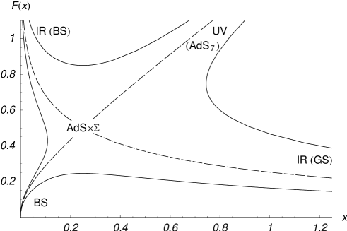
Figure 1. Behaviour of the orbits for five-branes wrapping SLAG 3-cycles with $l=-1$. Note the flow from the $AdS_{7}$-type region when $F,x$ are large to the IR fixed point and the flows to the good and bad singularities in the IR, IR(GS) and IR(BS), respectively.

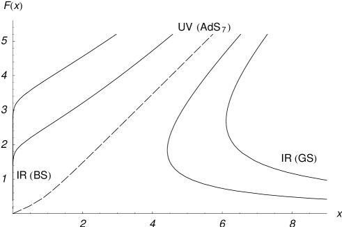
Figure 2. Behaviour of the orbits for fivebranes wrapping SLAG 3-cycles with $l=1$.

The typical behaviour of $F(x)$ is illustrated in figure 1 for $l=-1$ and figure 2 for $l=1$. The region where both $x$ and $F$ are large is interesting. There we have $F\approx x-l/m^{2}$ and using $a$ as a radial variable we obtain the asymptotic behaviour of the metric:

$$ds^{2}\approx\frac{4}{m^{2}a^{2}}da^{2}+a^{2}[ds^{2}(\mathbb{R}^{1,2})+d\bar{s}^{2}(\Sigma_{3})]\\ ~{}.$$

This looks very similar to $AdS_{7}$ in Poincare co-ordinates except that the sections with constant $a$ are not $\mathbb{R}^{1,5}$ but $\mathbb{R}^{1,2}\times\Sigma_{3}$.

This clearly corresponds to the near horizon limit of the fivebrane wrapped on the SLAG 3-cycle. By the general discussion on the AdS/CFT correspondence earlier, this should be dual to the six dimensional quantum field theory living on the wrapped fivebrane worldvolume $\mathbb{R}^{1,2}\times\Sigma_{3}$, after decoupling gravity. More precisely, the asymptotic behaviour of the solution (5.4), when lifted to D=11, is dual to the UV behaviour of the quantum field theory. Following the flow of the solution as in figures 1 and 2 correspond to flowing to the IR of the field theory. In the present context, the IR corresponds to length scales large compared to the size of the cycle $\Sigma_{3}$ on which the fivebrane is wrapped. In other words, going to the IR corresponds to taking $\Sigma_{3}$ to be very small (assuming it is compact) and the six dimensional quantum field theory on $\mathbb{R}^{1,2}\times\Sigma_{3}$ behaves more and more like a three-dimensional quantum field theory on $\mathbb{R}^{1,2}$.

Perhaps the most interesting solutions occur for $l=-1$. There is a solution indicated by one of the dashed lines in figure 1 that flows from the UV $AdS_{7}$ type region to the $AdS_{4}\times(H^{3}/\Gamma)$ fixed point that was given in (5.4). This is a supergravity solution that describes a kind of renormalisation group flow from a theory on $\mathbb{R}^{1,2}\times(H^{3}/\Gamma)$ to a superconformal field theory on $\mathbb{R}^{1,2}$. In particular, we see that the natural interpretation of the $AdS_{4}\times(H^{3}/\Gamma)$ solution is that, when it is lifted to D=11, it is dual to a superconformal field theory on $\mathbb{R}^{1,2}$ that arises as the IR limit of the fivebrane field theory on living on $\mathbb{R}^{1,2}\times(H^{3}/\Gamma)$. The interpretation for non-compact $H^{3}/\Gamma$ is less clear.

The absence of an $AdS_{4}\times(S^{3}/\Gamma)$ solution for $l=1$ possibly indicates that the quantum field theories arising on fivebranes wrapping SLAG 3-cycles with positive curvature are not superconformal in the infra-red. Alternatively, it could be that there are more elaborate solutions lying outside of our ansatz that have $AdS_{4}$ factors.

All other flows in figures 1 and 2 starting from the $AdS_{7}$ type region, flow to singular solutions. Being singular does not exclude the possibility that they might be interesting physically. Indeed, a criteria for time-like singularities in static geometries to be “good singularities”, i.e. dual to some quantum field theory behaviour, was presented in [110]. In particular, a good singularity is defined to be one in which the norm of the time-like Killing vector with respect to the D=11 supergravity metric does not increase as one goes to the singularity (one can also consider the weaker criteria that the norm is just bounded from above). It is not difficult to determine whether the singularities that arise in the different asymptotic limits are good or bad by this criteria and this has been presented in figures 1 and 2. It is likely that the good singularities describe some kind of Higgs branches of the quantum field theory corresponding to the possibility of moving the co-incident wrapped fivebranes apart.

In summary, using D=7 gauged supergravity, we have been able to construct D=11 supergravity solutions that describe fivebranes wrapping SLAG 3-cycles. The cycle is Einstein and is either $S^{3}/\Gamma$ or $H^{3}/\Gamma$ where $\Gamma$ is a discrete group of isometries. Probably the most important solutions that have been found are the $AdS_{4}\times(H^{3}/\Gamma)$ solutions which are dual to new superconformal field theories, after being uplifted to D=11. More general flow solutions were also constructed numerically.

5.5. Fivebranes wrapping other cycles

The construction of supersymmetric solutions corresponding to fivebranes wrapping other supersymmetric cycles runs along similar lines. The ansatz for the D=7 metric is given by

(5.31) $$ds^{2}=e^{2f}[ds^{2}(\mathbb{R}^{1,5-d})+dr^{2}]+e^{2g}d\bar{s}^{2}(\Sigma_{d})~{},$$

where $d\bar{s}^{2}_{d}$ is the metric on the supersymmetric $d$-cycle, $\Sigma_{d}$, and the functions $f$ and $g$ depend on the radial coordinate $r$ only.

The $SO(5)$-gauge fields are specified by the spin connection of the metric on $\Sigma_{d}$ in a way determined by the structure of the normal bundle of the calibrated cycle being wrapped. In general, we decompose the $SO(5)$ symmetry into $SO(p)\times SO(q)$ with $p+q=5$, and only excite the gauge fields in the $SO(p)$ subgroup. We will denote these directions by $a,b=1,\dots,p$. If we consider a probe fivebrane wrapping the cycle inside a manifold of special holonomy $M$, this decomposition corresponds to dividing the directions transverse to the brane into $p$ directions within $M$ and $q$ directions perpendicular to $M$. The precise ansatz for the $SO(p)$ gauge-fields is determined by some part of the spin connection on the cycle and will be discussed shortly.

In keeping with this decomposition, the solutions that we consider have a single scalar field excited. More precisely we take

(5.32) $${\Pi_{A}}^{i}=diag(e^{q\lambda},\dots,e^{q\lambda},e^{-p\lambda},\dots,e^{-p\lambda})~{},$$

where we have $p$ followed by $q$ entries. Once again this implies that the composite gauge-field $Q$ is then determined by the gauge-fields via $Q^{ab}=2mB^{ab}$.

It turns out that for the SLAG 5-cycle and most of the 4-cycle cases it is necessary to have non-vanishing three-forms $S_{A}$. The $S$-equation of motion is

(5.33) $$m^{2}\delta_{AC}{{\Pi^{-1}}_{i}}^{C}{{\Pi^{-1}}_{i}}^{B}S_{B}=-m*F_{A}+\frac{1}{4\sqrt{3}}\epsilon_{ABCDE}*(F^{BC}\wedge F^{DE})~{}.$$

The solutions have vanishing four-form field strength $F_{A}$ and hence $S_{A}$ are determined by the gauge fields.

Demanding that the configuration preserves supersymmetry, as for the SLAG 3-cycle case, we find that along the cycle directions:

(5.34) $$(\partial+\frac{1}{4}{\bar{\omega}}^{bc}\gamma_{bc}+\frac{m}{2}{B}^{ab}\Gamma_{ab})\epsilon=0~{},$$

where ${\bar{\omega}}^{bc}$ is the spin connection one-form of the cycle. For each case the specific gauge-fields, determined by the type of cycle being wrapped, go hand in hand with a set of projections which allow (5.34) to be satisfied for spinors independent of the coordinates along $\Sigma_{d}$. We can easily guess the appropriate ansatz for the gauge fields from our discussion of the structure of the normal bundles of calibrated cycles in section 4.1, and they are summarised below. The corresponding projections are then easily determined and are given explicitly in [110, 3, 71, 68]. In the uplifted D=11 solutions, these projections translate into a set of projections corresponding to those of the special holonomy manifold and an additional projection corresponding to the wrapped fivebrane.

By analysing the conditions for supersymmetry in more detail, one finds that the metric on the cycle is necessarily Einstein, and we again normalise so that

(5.35) $$\bar{R}_{ab}=l\bar{g}_{ab}~{},$$

with $l=0,\pm 1$. When $d=2,3$ the Einstein condition implies that the cycles have constant curvature and hence are either spheres, for $l=1$ or hyperbolic spaces for $l=1$, or quotients of these spaces by a discrete group of isometries. When $d>3$ the Einstein condition implies that the Riemann tensor can be written

(5.36) $$\bar{R}_{abcd}=\bar{W}_{abcd}+\frac{2l}{d-1}\bar{g}_{a[c}\bar{g}_{d]b}~{},$$

where ${\bar{W}}$ is the Weyl tensor, and there are more possibilities. By analysing the D=7 Einstein equations one finds that for $d=4,5$ the part of the spin connection that is identified with the gauge fields must have constant curvature.

We now summarise the ansatz for the $SO(5)$ gauge fields for each case and discuss the types of cycle that arise for $=4,5$. We can always take a quotient of the cycles listed by a discrete group of isometries.

SLAG $n$-cycles: Consider a probe fivebrane wrapping a SLAG $n$-cycle in a $CY_{n}$. The five directions transverse to the fivebrane consist of $n$ directions tangent to the $CY_{n}$ and $5-n$ normal to it. Thus, for the supergravity solution we decompose $SO(5)\to SO(n)\times SO(5-n)$, and let the only non-vanishing gauge fields lie in the $SO(n)$ factor. Up to a factor of $2m$ these $SO(n)$ gauge-fields are identified with $SO(n)$ spin connection on $\Sigma_{n}$, as in (5.16). This identification corresponds to the fact that $N(\Sigma_{n})\cong T(\Sigma_{n})$ for SLAG $n$-cycles. Since all of the spin connection is identified with the gauge-fields, the metric on $\Sigma_{n}$ must have constant curvature ($W=0$ for $d=4,5$) and hence $\Sigma_{n}$ is $S^{n}$ for $l=1$ and $H^{n}$ for $l=-1$.

Kähler 2-cycles: Kähler 2-cycles in $CY_{2}$ are SLAG 2-cycles and have just been discussed. For probe fivebranes wrapping Kähler 2-cycles in $CY_{3}$ the five directions transverse to the fivebrane consist of four directions tangent to the $CY_{3}$ and one flat direction normal to the $CY_{3}$. The normal bundle of the Kähler 2-cycle has structure group $U(2)\cong U(1)\times SU(2)$ and recall now (4.5). Thus, for the supergravity solution in D=7, we decompose $SO(5)\to SO(4)\to U(2)\cong U(1)\times SU(2)$ and identify the $U(1)$ spin connection of the cycle with the gauge-fields in the $U(1)$ factor. We also set the $SU(2)$ gauge-fields to zero, which corresponds to considering fivebranes wrapping Kähler 2-cycles with non-generic normal bundle. An example of such a cycle is the two-sphere in the resolved conifold. It would be interesting to find more general solutions with non-vanishing $SU(2)$ gauge-fields, preserving the same amount of supersymmetry.

Kähler-4-cycles: We assume that $\Sigma_{4}$ in the D=7 supergravity solution has a Kähler metric with a $U(2)\cong U(1)\times SU(2)$ spin connection. When probe fivebranes wrap Kähler 4-cycles in $CY_{3}$ the five transverse directions consist of two directions tangent to the $CY_{3}$ and three flat directions normal to the $CY_{3}$. Thus we decompose $SO(5)\to SO(2)\times SO(3)$, set the $SO(3)$ gauge-fields to zero and identify the $SO(2)\cong U(1)$ gauge fields with the $U(1)$ part of the $U(1)\times SU(2)$ spin connection on the 4-cycle. When probe fivebranes wrap Kähler 4-cycles in $CY_{4}$ the five transverse directions consist of four directions tangent to the $CY_{4}$ and one flat direction normal to the $CY_{4}$. Thus we now decompose $SO(5)\to SO(4)\to U(2)\cong U(1)\times SU(2)$ and we set the $SU(2)$ gauge-fields to zero, which again corresponds to considering non-generic normal bundles. We identify the $U(1)$ gauge-fields with the $U(1)$ part of the spin connection as dictated by (4.5). In both cases, the identification of the gauge fields with part of the spin connection doesn’t place any further constraints on $\Sigma_{4}$ other than it is Kähler-Einstein. An example when $l=1$ is $CP^{2}$.

$\mathbb{C}$-Lag 4-cycles: We again assume that $\Sigma_{4}$ in the D=7 solution has a Kähler metric with a $U(2)\cong U(1)\times SU(2)$ spin connection. We again decompose $SO(5)\to SO(4)\to U(2)\cong U(1)\times SU(2)$ but now we do not set the $SU(2)$ gauge-fields to zero. Indeed, since the cycle is both SLAG and Kähler, with respect to different complex structures, we must identify all of the $U(2)$ gauge-fields with the $U(2)$ spin connection. Einstein’s equations then imply that $\Sigma_{4}$ must have constant holomorphic sectional curvature. This means that for $l=1$ it is $CP^{2}$ while for $l=-1$ it is the open disc in $\mathbb{C}^{2}$ with the Bergman metric. Note that the solutions corresponding to fivebranes wrapping $\mathbb{C}$-Lag $CP^{2}$ are different from the solutions corresponding to fivebranes wrapping Kähler $CP^{2}$, since they have more gauge-fields excited and preserve different amounts of supersymmetry.

Associative 3-cycles: When probe fivebranes wrap associative 3-cycles in $G_{2}$ manifolds, there are four transverse directions that are tangent to the $G_{2}$ manifold and one flat direction normal to the $G_{2}$ manifold. We thus decompose $SO(5)\to SO(4)\cong SU(2)^{+}\times SU(2)^{-}$, where the superscripts indicate the self-dual and anti-self-dual parts. Recall that the normal bundle of associative 3-cycles is given by $S\otimes V$ where $S$ was the $SU(2)$ spin bundle on $\Sigma_{3}$ and $V$ is a rank $SU(2)$ bundle. In the non-generic case when $V$ is trivial, for example for the $G_{2}$ manifold in [28], then the identification of the gauge-fields is clear: we should identify the $SO(3)\cong SU(2)$ spin connection on $\Sigma_{3}$ with $SU(2)^{+}$ gauge-fields and set the $SU(2)^{-}$ gauge-fields to zero.

Co-associative 4-cycles: When probe fivebranes wrap co-associative 4-cycles in $G_{2}$ manifolds, there are three transverse directions that are tangent to the $G_{2}$ manifold and two flat directions normal to the $G_{2}$ manifold. We thus decompose $SO(5)\to SO(3)\times SO(2)$ and set the $SO(2)$ gauge-fields to zero. Recall that the normal bundle of co-associative 4-cycles is isomorphic to the bundle of anti-self-dual two-forms on the 4-cycle. This indicates that we should identify the $SO(3)\cong SU(2)$ gauge-fields with the anti-self-dual part, $SU(2)^{-}$, of the $SO(4)\cong SU(2)^{+}\times SU(2)^{-}$ spin connection on $\Sigma_{4}$. For the co-associative 4-cycles, Einstein’s equations imply that the anti-self-dual part of the spin connection has constant curvature, or in other words, the Weyl tensor is self-dual $W^{-}=0$. These manifolds are sometimes called conformally half-flat. If $l=1$ the only compact examples are $CP^{2}$ and $S^{4}$.

Cayley 4-cycles: When probe fivebranes wrap Cayley 4-cycles in $Spin(7)$ manifolds the five normal directions consist of four directions tangent to the $Spin(7)$ manifold and one flat direction normal to the $Spin(7)$ manifold. We thus again decompose $SO(5)\to SO(4)\cong SU(2)^{+}\times SU(2)^{-}$, where the superscripts indicate the self-dual and anti-self-dual parts. Recall that the normal bundle of Cayley 4-cycles is given by $S_{-}\otimes V$ where $S_{-}$ was the $SU(2)$ bundle of negative chirality spinors on $\Sigma_{3}$ and $V$ is a rank $SU(2)$ bundle. In the non-generic case when $V$ is trivial, for example for the $Spin(7)$ manifolds in [28], then the identification of the gauge-fields is clear: if $SU(2)^{\pm}$ are the self-dual and anti-self-dual parts of the $SO(4)$ spin connection on $\Sigma_{4}$ then we should identify the $SU(2)^{-}$ part of the spin connection with $SU(2)^{-}$ gauge fields and set the $SU(2)^{+}$ gauge-fields to zero. As for the co-associative 4-cycles, Einstein’s equations imply that the Weyl tensor is self-dual $W^{-}=0$.

With this data the BPS equations can easily be derived and we refer to [110, 3, 71, 68] for the explicit equations. They have a similar appearance to those of the SLAG 3-cycle case, with the addition of an extra term coming from the three-forms $S$ for most of the 4-cycle cases and the SLAG 5-cycles. When the curvature of the cycle is negative, $l=-1$, in all cases except for Kähler 4-cycles in $CY_{3}$, we obtain an $AdS_{7-d}\times\Sigma_{d}$ fixed point. When $l=1$, only for SLAG 5-cycles do we find such a fixed point. This is summarised in table 5.

We note that using exactly the same ansatz for the D=7 supergravity fields, some additional non-supersymmetric solutions of the form $AdS_{7-d}\times\Sigma_{d}$ were found [62]. In addition, by considering the possibility of extra scalar fields being excited, one more $AdS_{3}$ solution was found. Such solutions could be dual to non-supersymmetric conformal field theories, that are related to wrapped fivebranes with supersymmetry broken. To develop this interpretation it is necessary that the solutions are stable, which is difficult to determine. A preliminary perturbative investigation revealed that some of these solutions are unstable. We have also summarised these solutions in table 5.

spacetime	embedding	cycle $\Sigma_{n}$	supersymmetry
$AdS_{5}\times\Sigma_{2}$	Kähler 2-cycle in $CY_{2}$	$H^{2}$	yes
		$S^{2}$	no∗
	Kähler 2-cycle in $CY_{3}$	$H^{2}$	yes
		$H^{2}$	no
$AdS_{4}\times\Sigma_{3}$	SLAG 3-cycle in $CY_{3}$	$H^{3}$	yes
		$H^{3}$	no
	Associative 3-cycle	$H^{3}$	yes
		$H^{3}$	no
$AdS_{3}\times\Sigma_{4}$	Coassociative 4-cycle	$C_{-}^{4}$	yes
	SLAG 4-cycle in $CY_{4}$	$H^{4}$	yes
		$H^{4}$	no
		$S^{4}$	no
	Kähler 4-cycle in $CY_{4}$	$K_{-}^{4}$	yes
		$K_{+}^{4}$	no
	Cayley 4-cycle	$C_{-}^{4}$	yes
		$C_{-}^{4}$	no
		$CP^{2},S^{4}$	no
	CLAG 4-cycle in $HK_{8}$	$B$	yes
		$B$	no
		$CP^{2}$	no
	SLAG 4-cycle in $CY_{2}\times CY_{2}$	$H^{2}\times H^{2}$	yes
		$H^{2}\times H^{2}$	no∗
		$S^{2}\times S^{2}$	no∗
		$S^{2}\times H^{2}$	no∗
$AdS_{2}\times\Sigma_{5}$	SLAG 5-cycle in $CY_{5}$	$H^{5}$	yes
		$S^{5}$	yes
	SLAG 5-cycle in $CY_{2}\times CY_{3}$	$H^{3}\times H^{2}$	yes
		$S^{2}\times H^{3}$	no
		$S^{2}\times H^{3}$	no

Table 5. $AdS$ fixed point solutions for wrapped fivebranes: $C_{-}$ and $K_{\pm}$ are conformally half-flat and Kähler–Einstein metrics with the subscript denoting positive or negative scalar curvature and $B$ is the Bergmann metric. Note that we can also take quotients of all cycles by discrete groups of isometries and this preserves supersymmetry. ^∗ denotes a solution shown to be unstable.

5.6. Wrapped Membranes and D3-branes

D=11 supergravity solutions describing membranes wrapping Kähler 2-cycles can be found in an analogous manner [70]. The appropriate gauged supergravity for this case is maximal $SO(8)$ gauged supergravity in D=4 [47, 48] which can be obtained from a consistent truncation of the dimensional reduction of D=11 supergravity on a seven sphere [50, 49]. The vacuum solution of this theory is $AdS_{4}$ and this uplifts to $AdS_{4}\times S^{7}$, which is the near horizon limit of the planar membrane solution. More general solutions can be found that uplift to solutions describing the near horizon limit of wrapped membranes.

Actually, the general formulae for obtaining $SO(8)$ gauged supergravity from the dimensional reduction of D=11 supergravity on the seven sphere are rather implicit and not in a form that is useful for uplifting general solutions. Luckily, there is a further consistent truncation of the $SO(8)$ gauged supergravity theory to a $U(1)^{4}$ gauged supergravity where the formulae are known explicitly (in the special case that the axion fields are zero) [39] and this is sufficient for the construction of D=11 wrapped membrane solutions.

To see why, let us describe the ansatz for the gauge-fields for the D=4 solutions. If we consider a probe membrane wrapping a Kähler 2-cycle in a $CY_{n}$ then the eight directions transverse to the membrane consist of $2n-2$ directions that are tangent to the $CY_{n}$ and $10-2n$ flat directions that are normal to the $CY_{n}$. In addition the normal bundle of the Kähler 2-cycle in $CY_{n}$ has structure group $U(n-1)\cong U(1)\times SU(n-1)$ and recall (4.5). Thus, in the D=4 supergravity, we should first decompose $SO(8)\to SO(2n-2)\times SO(10-2n)$ and only have non-vanishing gauge fields in $U(n-1)\subset SO(2n-2)$. The gauge-fields in the $U(1)$ factor of $U(n-1)\cong U(1)\times SU(n-1)$ are then identified with the $U(1)$ spin connection on the 2-cycle, corresponding to (4.5). In the solutions that have been constructed, the remaining $SU(n-1)$ gauge-fields are set to zero, which corresponds to the normal bundle of the Kähler 2-cycle being non-generic when $n\geq 3$. Thus, the ansatz for the gauge fields are such that they always lie within the maximal cartan subalgebra $U(1)^{4}$ of $SO(8)$ and hence the truncation formulae of [39] can be used.

Once again the metric on the 2-cycle is Einstein and hence is either $S^{2}/\Gamma$ for $l=1$ or $H^{2}/\Gamma$ for $l=-1$. In particular, the cycle can be an arbitrary Riemann surface. General BPS equations have been found and analysed numerically. Interestingly, $AdS_{2}\times\Sigma_{2}$ fixed points are found only for $l=-1$ and only for the cases of $CY_{4}$ and $CY_{5}$. When uplifted to D=11 these solutions become a warped product with a non-round seven sphere that is non-trivially fibred over the cycle. The $AdS_{2}$ fixed point solutions should be dual to superconformal quantum mechanics living on the wrapped membranes.

The appropriate gauged supergravity theory for finding D=10 type IIB solutions describing D3-branes wrapping various calibrated cycles, is the maximally supersymmetric $SO(6)$ gauged supergravity in D=5 [85]. This can be obtained from the consistent truncation of the dimensional reduction of the type IIB supergravity on a five-sphere. In particular, the vacuum solution is $AdS_{5}$ and this uplifts to $AdS_{5}\times S^{5}$ which is the near horizon limit of the planar D3-brane. Actually the general formulae for this reduction are not yet known and one has to exploit further consistent truncations that are known [129, 39, 107, 43].

All cases in table 3 have been investigated, and BPS equations have been found and analysed. Once again, in the solutions, the 2- and 3-cycles that the D3-branes wrap have Einstein metrics and hence have constant curvature. D3-branes wrapping Kähler 2-cycles in $CY_{2}$ and $CY_{3}$ were studied in [110] while the $CY_{4}$ case was analysed in [115]. $AdS_{3}\times H^{2}/\Gamma$ fixed points were found for the $CY_{3}$ and $CY_{4}$ cases. D3-branes wrapping associative 3-cycles were analysed in [118] and an $AdS_{2}\times H^{3}/\Gamma$ fixed point was found. Finally, D3-branes wrapping SLAG 3-cycles were studied in [115] and no $AdS_{2}$ fixed point was found. Note that non-supersymmetric $AdS$ solutions were sought in [115] for both wrapped membranes and D3-branes, generalising the fivebrane solutions in [62], but none were found.

5.7. Other wrapped brane solutions

Let us briefly mention some other supergravity solutions describing wrapped branes that have been constructed.

D6-branes of type IIA string theory carry charge under the $U(1)$ gauge-field arising from the Kaluza-Klein reduction of D=11 supergravity on an $S^{1}$ (the field $C^{(1)}$ in (5.2)). The planar D6-brane uplifts to pure geometry: $\mathbb{R}^{1,6}\times M_{4}$ where $M_{4}$ is Taub-NUT space with $SU(2)$ holonomy. Similarly, when D6-branes wrap calibrated cycles they uplift to other special holonomy manifolds in D=11 and this has been studied in e.g. [1, 8, 80, 53, 91, 82]. Other solutions related to wrapped D6-branes that are dual to non-commutative field theories have been studied in [25, 26].

There are solutions of massive type IIA supergravity with $AdS_{6}$ factors which are dual to the five-dimensional conformal field theory arising on the D4-D8-brane system [56, 23]. Supersymmetric and non-supersymmetric solutions describing the D4-D8 system wrapped on various calibrated cycles were found in [119, 115].

For some other supergravity solutions with possible applications to AdS/CFT, that are somewhat related to those described here, see [7, 41, 54, 55, 24, 32, 105, 31, 106].

6. Discussion

We have explained in some detail the construction of supergravity solutions describing branes wrapping calibrated cycles. There are a number of issues that are worth further investigation.

It seems plausible that the BPS equations can be solved exactly. To date this has only been achieved in a few cases. They were solved for the case of membranes wrapping Kähler 2-cycles in $CY_{5}$ [70], but this case is special in that all scalar fields in the gauged supergravity are set to zero. When there is a non-vanishing scalar field, the BPS equations were solved exactly for some cases in [110] and they have been partially integrated for other cases. Of particular interest are the exact solutions corresponding to the flows from an $AdS_{D}$ region to an $AdS_{D-d}\times\Sigma_{d}$ fixed point (for example, one of the dashed lines in figure 1) as they are completely regular solutions.

For the case of membranes wrapping Kähler 2-cycles in $CY_{5}$, the general flow solution can be viewed as the “topological” $AdS_{4}$ black holes discussed in [29]. When $l=-1$, there is a supersymmetric rotating generalisation of this black hole [29]: when it uplifted to D=11, it corresponds to waves on the wrapped membrane [70]. The rotating solution is completely regular provided that the angular momentum is bounded. It would be interesting to understand this bound from the point of view of the dual field theory. In addition, the existence of this rotating solution suggests that for all of the regular flow solutions of wrapped branes starting from an $AdS_{D}$ region and flowing to an $AdS_{D-d}\times\Sigma_{d}$ region, there should be rotating generalisations that are waiting to be found.

In all of the supergravity solutions describing wrapped branes that have been constructed, the cycle has an Einstein metric on it. It would be interesting if a more general ansatz could be found in which this condition is relaxed. While this seems possible, it may not be possible to find explicit solutions. In some cases, such as fivebranes wrapping Kähler 2-cycles in $CY_{3}$, we noted that the solutions constructed correspond to fivebranes wrapping cycles with non-generic normal bundles. This was because certain gauge-fields were set to zero. We expect that more general solutions can be found corresponding to generic normal bundles. Note that such a solution, with an AdS factor, was found for D3-branes wrapping Kähler 2-cycles in $CY_{3}$ [110].

It would also be interesting to construct more general solutions that describe the wrapped branes beyond the near horizon limit. Such solutions would asymptote to a special holonomy manifold, which would necessarily be non-compact in order that the solution can carry non-zero flux (a no-go theorem for D=11 supergravity solutions with flux is presented in [76]). It seems likely that solutions can be found that asymptote to the known co-homogeneity-one special holonomy manifolds. For example, the deformed conifold is a co-homogeneity-one $CY_{3}$ that is a regular deformation of the conifold. It has a SLAG three-sphere and topologically the manifold is the co-tangent bundle of the three-sphere, $T^{*}(S^{3})$. It should be possible to generalise the solutions describing fivebranes wrapping SLAG three-spheres in the near horizon limit, to solutions that include an asymptotic region far from the branes that approaches the conifold metric. Of course, these solutions will still be singular in the near horizon limit. It will be particularly interesting to construct similar solutions for the $l=-1$ case. $T^{*}(H^{3})$ admits a $CY_{3}$ metric, with a SLAG $H^{3}$ but there is a singularity at some finite distance from the SLAG 3-cycle. There may be a solution with non-zero flux that interpolates from this singular behaviour down to the regular near horizon solutions that we constructed. Alternatively, it may be that the flux somehow “pushes off” the singularity to infinity and the entire solution is regular. The construction of these more general solutions, when the four-sphere transverse to the fivebrane is allowed to get large, will necessarily require new techniques, as they cannot be found in the gauged supergravity.

The construction of the wrapped brane solutions using gauged supergravity is rather indirect and it is desirable to characterise the D=11 geometries more directly. For example, this may lead to new methods to generalise the solutions along the lines mentioned above. One approach, is to guess general ansatzë for D=11 supergravity configurations that might describe wrapped brane solutions and then impose the conditions to have supersymmetry. This approach has its origins in the construction of the intersecting brane solutions, reviewed in [64, 133], and was further extended in e.g. [54, 35, 98, 99]. Recently, it has been appreciated that it is possible to systematically characterise supersymmetric solutions of supergravity theories with non-zero fluxes using the notion of $G$-structures [67, 60, 101, 74, 76, 75] (see also [66, 63]). In particular, it was emphasised in some of these works that generalised calibrations play a central role and this is intimately connected with the fact that supergravity solutions with non-vanishing fluxes arise when branes wrap calibrated cycles. It should be noted that while these techniques provide powerful ways of characterising the D=11 geometries it is often difficult to obtain explicit examples: indeed even recovering the known explicit solutions found via gauged supergravity can be non-trivial (see e.g. [74]).

The supergravity solutions can be used to learn a lot about the dual conformal field theory, assuming the AdS/CFT correspondence is valid. For example, the $AdS$ fixed points can be used to determine the spectrum and correlation functions of the operators in the dual field theory. For the case of wrapped D3-branes, since the dual field theory is related to ${\mathcal{N}}=4$ super Yang-Mills theory, some detailed comparisons can be made [110]. For the fivebrane case it will be more difficult to do this since the conformal field theory living on the fivebrane is still poorly understood. Perhaps some detailed comparisons can be made for the wrapped membranes.

Recently some new supersymmetric solutions with AdS factors were constructed in [38, 37]. It will be interesting to determine their dual CFT interpretation and to see if they are related to wrapped branes. The non-supersymmetric solutions containing AdS factors found in [62] might be dual to non-supersymmetric conformal field theories. A necessary requirement is that the solutions are stable: it would be useful to complete the preliminary analysis of the perturbative stability undertaken in [62].

Supergravity solutions that are dual to supersymmetric quantum field theories that are not conformally invariant can be constructed using wrapped $NS$ 5-branes of type IIB string theory. The near horizon limit of the planar $NS$ 5-brane is dual to what is known as “little string theory” in six dimensions (for a review see [4]). These still mysterious theories are not local quantum field theories but at low-energies they give rise to supersymmetric Yang-Mills (SYM) theory in six dimensions. As a consequence, the geometries describing $NS$ 5-branes wrapped on various calibrated cycles encode information about various SYM theories in lower-dimensions. The geometries describing $NS$ 5-branes wrapped on Kähler 2-cycles in $CY_{3}$ were constructed in [34, 111] and are dual to ${\mathcal{N}}=1$ SYM theory in four dimensions. If the 5-branes are wrapped on Kähler 2-cycles in $CY_{2}$ the geometries are dual to ${\mathcal{N}}=2$ SYM theory in four dimensions [69, 22] (see also [94]). By wrapping on associative 3-cycles one finds geometries that encode information about ${\mathcal{N}}=1$ SYM in D=3 [3, 34, 130, 109, 81], while wrapping on SLAG 3-cycles one finds ${\mathcal{N}}=2$ SYM in D=3 [67, 83]. For the latter case, the solutions presented in [67, 83] are singular and correspond to vanishing Chern-Simons form in the dual SYM theory. There are strong physical arguments that suggest there are more general regular solutions that are dual to SYM with non-vanishing Chern-Simons form, and it would be very interesting to construct them. Note that supergravity solutions describing $NS$ 5-branes wrapping various 4-cycles were found in [115]. The D=10 geometry for wrapped $NS$ 5-branes has been analysed in some detail in [61, 67, 60, 101, 74, 75].

We hope to have given the impression that while much is now known about supergravity solutions describing branes wrapped on calibrated cycles, there is still much to be understood.

References

- [1] B.S. Acharya, On realising N = 1 super Yang-Mills in M theory, hep-th/0011089.
- [2] B.S. Acharya, J.M. Figueroa-O’Farrill, C.M. Hull, and B. Spence, Branes at conical singularities and holography, Adv. Theor. Math. Phys. 2 (1999), 1249–1286.
- [3] B.S. Acharya, J.P. Gauntlett, and N. Kim, Fivebranes wrapped on associative three-cycles, Phys. Rev. D63 (2001), 106003.
- [4] O. Aharony, A brief review of ’little string theories’, Class. Quant. Grav. 17 (2000), 929–938.
- [5] by same author, The non-AdS/non-CFT correspondence, or three different paths to QCD, hep-th/0212193.
- [6] O. Aharony, S.S. Gubser, J.M. Maldacena, H. Ooguri, and Y. Oz, Large N field theories, string theory and gravity, Phys. Rept. 323 (2000), 183–386.
- [7] M. Alishahiha and Y. Oz, AdS/CFT and BPS strings in four dimensions, Phys. Lett. B465 (1999), 136–141.
- [8] M. Atiyah, J.M. Maldacena, and C. Vafa, An M-theory flop as a large N duality, J. Math. Phys. 42 (2001), 3209–3220.
- [9] M. Atiyah and E. Witten, M-theory dynamics on a manifold of G(2) holonomy, Adv. Theor. Math. Phys. 6 (2003), 1–106.
- [10] I. Bandos, K. Lechner, A. Nurmagambetov, P. Pasti, D.P. Sorokin, and M. Tonin, Covariant action for the super-five-brane of M-theory, Phys. Rev. Lett. 78 (1997), 4332–4334.
- [11] O. Barwald, N.D. Lambert, and P.C. West, A calibration bound for the M-theory fivebrane, Phys. Lett. B463 (1999), 33–40.
- [12] K. Becker, M. Becker, and A. Strominger, Five-branes, membranes and nonperturbative string theory, Nucl. Phys. B456 (1995), 130–152.
- [13] Katrin Becker, M. Becker, D.R. Morrison, H. Ooguri, Y. Oz, and Z. Yin, Supersymmetric cycles in exceptional holonomy manifolds and Calabi-Yau 4-folds, Nucl. Phys. B480 (1996), 225–238.
- [14] E. Bergshoeff, R. Kallosh, T. Ortin, and G. Papadopoulos, kappa-symmetry, supersymmetry and intersecting branes, Nucl. Phys. B502 (1997), 149–169.
- [15] E. Bergshoeff, E. Sezgin, and P.K. Townsend, Supermembranes and eleven-dimensional supergravity, Phys. Lett. B189 (1987), 75–78.
- [16] by same author, Properties of the eleven-dimensional super membrane theory, Ann. Phys. 185 (1988), 330.
- [17] E. Bergshoeff, D.P. Sorokin, and P.K. Townsend, The M5-brane hamiltonian, Nucl. Phys. B533 (1998), 303–316.
- [18] M. Bershadsky, C. Vafa, and V. Sadov, D-branes and topological field theories, Nucl. Phys. B463 (1996), 420–434.
- [19] M. Bertolini, Four lectures on the gauge-gravity correspondence, hep-th/0303160.
- [20] M. Bertolini, P. Di Vecchia, M. Frau, A. Lerda, R. Marotta, and I. Pesando, Fractional D-branes and their gauge duals, JHEP 02 (2001), 014.
- [21] F. Bigazzi, A.L. Cotrone, M. Petrini, and A. Zaffaroni, Supergravity duals of supersymmetric four dimensional gauge theories, hep-th/0303191.
- [22] F. Bigazzi, A.L. Cotrone, and A. Zaffaroni, N = 2 gauge theories from wrapped five-branes, Phys. Lett. B519 (2001), 269–276.
- [23] A. Brandhuber and Y. Oz, The D4-D8 brane system and five dimensional fixed points, Phys. Lett. B460 (1999), 307–312.
- [24] B. Brinne, A. Fayyazuddin, S. Mukhopadhyay, and D.J. Smith, Supergravity M5-branes wrapped on Riemann surfaces and their QFT duals, JHEP 12 (2000), 013.
- [25] J. Brugues, J. Gomis, T. Mateos, and T. Ramirez, Commutative and noncommutative N = 2 SYM in 2+1 from wrapped D6-branes, hep-th/0212179.
- [26] by same author, Supergravity duals of noncommutative wrapped D6 branes and supersymmetry without supersymmetry, JHEP 10 (2002), 016.
- [27] R.L. Bryant, Pseudo-Riemannian metrics with parallel spinor fields and vanishing Ricci tensor, Global analysis and harmonic analysis (Marseille-Luminy, 1999), Sémin. Congr., vol. 4, Soc. Math. France, Paris, 2000, pp. 53–94.
- [28] R.L. Bryant and S.M. Salamon, On the construction of some complete metrics with exceptional holonomy, Duke Math. J. 58 (1989), no. 3, 829–850.
- [29] M.M. Caldarelli and D. Klemm, Supersymmetry of anti-de sitter black holes, Nucl. Phys. B545 (1999), 434–460.
- [30] I.C.G. Campbell and P.C. West, N=2 D = 10 nonchiral supergravity and its spontaneous compactification, Nucl. Phys. B243 (1984), 112.
- [31] A.H. Chamseddine and W.A. Sabra, Magnetic and dyonic black holes in D = 4 gauged supergravity, Phys. Lett. B485 (2000), 301–307.
- [32] by same author, Magnetic strings in five dimensional gauged supergravity theories, Phys. Lett. B477 (2000), 329–334.
- [33] A.H. Chamseddine and M.S. Volkov, Non-abelian solitons in N = 4 gauged supergravity and leading order string theory, Phys. Rev. D57 (1998), 6242–6254.
- [34] by same author, Non-abelian vacua in d = 5, N = 4 gauged supergravity, JHEP 04 (2001), 023.
- [35] H. Cho, M. Emam, D. Kastor and J. Traschen, Calibrations and Fayyazuddin-Smith spacetimes, Phys. Rev. D 63 (2001) 064003.
- [36] E. Cremmer, B. Julia, and J. Scherk, Supergravity theory in 11 dimensions, Phys. Lett. B76 (1978), 409–412.
- [37] S. Cucu, H. Lu, and J.F. Vazquez-Poritz, Interpolating from AdSD-2 S2 to AdSD, hep-th/0304022.
- [38] by same author, A supersymmetric and smooth compactification of M-theory to AdS5, hep-th/0303211.
- [39] M. Cvetic, M.J. Duff, P. Hoxha, J.T. Liu, H. Lu, J.X. Lu, R. Martinez-Acosta, C.N. Pope, H. Sati, and T.A. Tran, Embedding AdS black holes in ten and eleven dimensions, Nucl. Phys. B558 (1999), 96–126.
- [40] M. Cvetic, G.W. Gibbons, H. Lu, and C.N. Pope, Special holonomy spaces and M-theory, hep-th/0206154.
- [41] M. Cvetic, H. Lu, C. N. Pope, and J. F. Vazquez-Poritz, AdS in warped spacetimes, Phys. Rev. D62 (2000), 122003.
- [42] M. Cvetic, H. Lu, and C.N. Pope, Brane resolution through transgression, Nucl. Phys. B600 (2001), 103–132.
- [43] M. Cvetic, H. Lu, C.N. Pope, A. Sadrzadeh, and T.A. Tran, Consistent SO(6) reduction of type IIB supergravity on S5, Nucl. Phys. B586 (2000), 275–286.
- [44] J. Dadok and R. Harvey, Calibrations and spinors, Acta Math. 170 (1993), no. 1, 83–120.
- [45] J. Dadok, R. Harvey, and F. Morgan, Calibrations on , Trans. Amer. Math. Soc. 307 (1988), no. 1, 1–40.
- [46] S.P. de Alwis, A note on brane tension and M-theory, Phys. Lett. B388 (1996), 291–295.
- [47] B. de Wit and H. Nicolai, N=8 supergravity, Nucl. Phys. B208 (1982), 323.
- [48] by same author, N=8 supergravity with local SO(8)SU(8) invariance, Phys. Lett. B108 (1982), 285.
- [49] by same author, The consistency of the truncation in d = 11 supergravity, Nucl. Phys. B281 (1987), 211.
- [50] B. de Wit, H. Nicolai, and N.P. Warner, The embedding of gauged N=8 supergravity into d = 11 supergravity, Nucl. Phys. B255 (1985), 29.
- [51] M.J. Duff and J.T. Liu, Hidden spacetime symmetries and generalized holonomy in M- theory, hep-th/0303140.
- [52] M.J. Duff, J.T. Liu, and R. Minasian, Eleven-dimensional origin of string / string duality: A one-loop test, Nucl. Phys. B452 (1995), 261–282.
- [53] J.D. Edelstein and C. Nunez, D6 branes and M-theory geometrical transitions from gauged supergravity, JHEP 04 (2001), 028.
- [54] A. Fayyazuddin and D.J. Smith, Localized intersections of M5-branes and four-dimensional superconformal field theories, JHEP 04 (1999), 030.
- [55] by same author, Warped AdS near-horizon geometry of completely localized intersections of M5-branes, JHEP 10 (2000), 023.
- [56] S. Ferrara, A. Kehagias, H. Partouche, and A. Zaffaroni, AdS6 interpretation of 5D superconformal field theories, Phys. Lett. B431 (1998), 57–62.
- [57] J.M. Figueroa-O’Farrill, Breaking the M-waves, Class. Quant. Grav. 17 (2000), 2925–2948.
- [58] J.M. Figueroa-O’Farrill and G. Papadopoulos, Maximally supersymmetric solutions of ten-dimensional and eleven-dimensional supergravities, hep-th/0211089.
- [59] D.Z. Freedman, S.S. Gubser, K. Pilch, and N.P. Warner, Renormalization group flows from holography supersymmetry and a c-theorem, Adv. Theor. Math. Phys. 3 (1999), 363–417.
- [60] T. Friedrich and S. Ivanov, Killing spinor equations in dimension 7 and geometry of integrable -manifolds, math.dg/0112201.
- [61] by same author, Parallel spinors and connections with skew-symmetric torsion in string theory, Asian J. Math. 6 (2001), no. 2, 303–335.
- [62] J. P. Gauntlett, N. Kim, S. Pakis, and D. Waldram, M-theory solutions with AdS factors, Class. Quant. Grav. 19 (2002), 3927–3946.
- [63] J.P. Gauntlett and J.B. Gutowski, All supersymmetric solutions of minimal gauged supergravity in five dimensions, hep-th/0304064.
- [64] J.P. Gauntlett, Intersecting branes, hep-th/9705011.
- [65] by same author, Membranes on fivebranes, Adv. Theor. Math. Phys. 3 (1999), 775–790.
- [66] J.P. Gauntlett, J.B. Gutowski, C.M. Hull, Stathis Pakis, and H.S. Reall, All supersymmetric solutions of minimal supergravity in five dimensions, hep-th/0209114.
- [67] J.P. Gauntlett, Kim, D. N., Martelli, and D. Waldram, Fivebranes wrapped on SLAG three-cycles and related geometry, JHEP 11 (2001), 018.
- [68] J.P. Gauntlett and N. Kim, M-fivebranes wrapped on supersymmetric cycles II, Phys. Rev. D65 (2002), 086003.
- [69] J.P. Gauntlett, N. Kim, D. Martelli, and D. Waldram, Wrapped fivebranes and N = 2 super Yang-Mills theory, Phys. Rev. D64 (2001), 106008.
- [70] J.P. Gauntlett, N. Kim, S. Pakis, and D. Waldram, Membranes wrapped on holomorphic curves, Phys. Rev. D65 (2002), 026003.
- [71] J.P. Gauntlett, N. Kim, and D. Waldram, M-fivebranes wrapped on supersymmetric cycles, Phys. Rev. D63 (2001), 126001.
- [72] J.P. Gauntlett, N.D. Lambert, and P. C. West, Supersymmetric fivebrane solitons, Adv. Theor. Math. Phys. 3 (1999), 91–118.
- [73] J.P. Gauntlett, N.D. Lambert, and P.C. West, Branes and calibrated geometries, Commun. Math. Phys. 202 (1999), 571–592.
- [74] J.P. Gauntlett, D. Martelli, S. Pakis, and D. Waldram, G-structures and wrapped NS5-branes, hep-th/0205050.
- [75] J.P. Gauntlett, D. Martelli, and D. Waldram, Superstrings with intrinsic torsion, hep-th/0302158.
- [76] J.P. Gauntlett and S. Pakis, The geometry of D= 11 Killing spinors, JHEP 0304 (2003) 039.
- [77] F. Giani and M. Pernici, N=2 supergravity in ten-dimensions, Phys. Rev. D30 (1984), 325–333.
- [78] G.W. Gibbons, G.T. Horowitz, and P.K. Townsend, Higher dimensional resolution of dilatonic black hole singularities, Class. Quant. Grav. 12 (1995), 297–318.
- [79] G.W. Gibbons and G. Papadopoulos, Calibrations and intersecting branes, Commun. Math. Phys. 202 (1999), 593–619.
- [80] J. Gomis, D-branes, holonomy and M-theory, Nucl. Phys. B606 (2001), 3–17.
- [81] by same author, On SUSY breaking and SB from string duals, Nucl. Phys. B624 (2002), 181–199.
- [82] J. Gomis and T. Mateos, D6 branes wrapping Kaehler four-cycles, Phys. Lett. B524 (2002), 170–176.
- [83] J. Gomis and J.G. Russo, D = 2+1 N = 2 Yang-Mills theory from wrapped branes, JHEP 10 (2001), 028.
- [84] S. S. Gubser, I. R. Klebanov and A. M. Polyakov, Gauge theory correlators from non-critical string theory, Phys. Lett. B 428 (1998), 105-114.
- [85] M. Gunaydin, L.J. Romans, and N.P. Warner, Compact and noncompact gauged supergravity theories in five-dimensions, Nucl. Phys. B272 (1986), 598.
- [86] J. Gutowski, S. Ivanov, and G. Papadopoulos, Deformations of generalized calibrations and compact non-Kahler manifolds with vanishing first Chern class, (2002).
- [87] J. Gutowski and G. Papadopoulos, AdS calibrations, Phys. Lett. B462 (1999), 81–88.
- [88] J. Gutowski, G. Papadopoulos, and P.K. Townsend, Supersymmetry and generalized calibrations, Phys. Rev. D60 (1999), 106006.
- [89] R. Harvey, Spinors and calibrations, Perspectives in Mathematics, vol. 9, Academic Press Inc., Boston, MA, 1990.
- [90] R. Harvey and H.B. Lawson, Jr., Calibrated geometries, Acta Math. 148 (1982), 47–157.
- [91] R. Hernandez, Branes wrapped on coassociative cycles, Phys. Lett. B521 (2001), 371–375.
- [92] P. Horava and E. Witten, Eleven-dimensional supergravity on a manifold with boundary, Nucl. Phys. B475 (1996), 94–114.
- [93] by same author, Heterotic and type I string dynamics from eleven dimensions, Nucl. Phys. B460 (1996), 506–524.
- [94] K. Hori and A. Kapustin, Worldsheet descriptions of wrapped NS five-branes, JHEP 11 (2002), 038.
- [95] P.S. Howe and E. Sezgin, D = 11, p = 5, Phys. Lett. B394 (1997), 62–66.
- [96] P.S. Howe, E. Sezgin, and P.C. West, Covariant field equations of the M-theory five-brane, Phys. Lett. B399 (1997), 49–59.
- [97] P.S. Howe and P.C. West, The complete N=2, d = 10 supergravity, Nucl. Phys. B238 (1984), 181.
- [98] T. Z. Husain, M2-branes wrapped on holomorphic curves, hep-th/0211030.
- [99] by same author, That’s a wrap!, hep-th/0302071.
- [100] M. Huq and M.A. Namazie, Kaluza-Klein supergravity in ten-dimensions, Class. Quant. Grav. 2 (1985), 293.
- [101] S. Ivanov, Connection with torsion, parallel spinors and geometry of Spin(7) manifolds, math.dg/0111216.
- [102] A. Khavaev, K. Pilch, and N.P. Warner, New vacua of gauged N = 8 supergravity in five dimensions, Phys. Lett. B487 (2000), 14–21.
- [103] I. R. Klebanov and E. Witten, Superconformal field theory on threebranes at a calabi-yau singularity, Nucl. Phys. B536 (1998), 199–218.
- [104] I.R. Klebanov and M.J. Strassler, Supergravity and a confining gauge theory: Duality cascades and SB-resolution of naked singularities, JHEP 08 (2000), 052.
- [105] D. Klemm and W.A. Sabra, Supersymmetry of black strings in D = 5 gauged supergravities, Phys. Rev. D62 (2000), 024003.
- [106] by same author, Charged rotating black holes in 5d Einstein-Maxwell-(A)dS gravity, Phys. Lett. B503 (2001), 147–153.
- [107] H. Lu, C.N. Pope, and T.A. Tran, Five-dimensional N = 4, SU(2) U(1) gauged supergravity from type IIB, Phys. Lett. B475 (2000), 261–268.
- [108] J.M. Maldacena, The large N limit of superconformal field theories and supergravity, Adv. Theor. Math. Phys. 2 (1998), 231–252.
- [109] J.M. Maldacena and H. Nastase, The supergravity dual of a theory with dynamical supersymmetry breaking, JHEP 09 (2001), 024.
- [110] J.M. Maldacena and C. Nunez, Supergravity description of field theories on curved manifolds and a no go theorem, Int. J. Mod. Phys. A16 (2001), 822–855.
- [111] by same author, Towards the large N limit of pure N = 1 super Yang Mills, Phys. Rev. Lett. 86 (2001), 588–591.
- [112] M. Marino, R. Minasian, G.W. Moore, and A. Strominger, Nonlinear instantons from supersymmetric p-branes, JHEP 01 (2000), 005.
- [113] R.C. McLean, Deformations of calibrated submanifolds, Comm. Anal. Geom. 6 (1998), no. 4, 705–747.
- [114] David R. Morrison and M. Ronen Plesser, Non-spherical horizons. I, Adv. Theor. Math. Phys. 3 (1999), 1–81.
- [115] M. Naka, Various wrapped branes from gauged supergravities, hep-th/0206141.
- [116] H. Nastase, D. Vaman, and P. van Nieuwenhuizen, Consistent nonlinear KK reduction of 11d supergravity on AdS7 S4 and self-duality in odd dimensions, Phys. Lett. B469 (1999), 96–102.
- [117] by same author, Consistency of the AdS7 S4 reduction and the origin of self-duality in odd dimensions, Nucl. Phys. B581 (2000), 179–239.
- [118] H. Nieder and Y. Oz, Supergravity and D-branes wrapping special lagrangian cycles, JHEP 03 (2001), 008.
- [119] C. Nunez, I.Y. Park, M. Schvellinger, and T.A. Tran, Supergravity duals of gauge theories from F(4) gauged supergravity in six dimensions, JHEP 04 (2001), 025.
- [120] G. Papadopoulos and A. Teschendorff, Multi-angle five-brane intersections, Phys. Lett. B443 (1998), 159–166.
- [121] by same author, Grassmannians, calibrations and five-brane intersections, Class. Quant. Grav. 17 (2000), 2641–2662.
- [122] P. Pasti, D.P. Sorokin, and M. Tonin, Covariant action for a D = 11 five-brane with the chiral field, Phys. Lett. B398 (1997), 41–46.
- [123] M. Pernici, K. Pilch, and P. van Nieuwenhuizen, Gauged maximally extended supergravity in seven-dimensions, Phys. Lett. B143 (1984), 103.
- [124] M. Pernici and E. Sezgin, Spontaneous compactification of seven-dimensional supergravity theories, Class. Quant. Grav. 2 (1985), 673.
- [125] K. Pilch and N.P. Warner, N = 2 supersymmetric RG flows and the IIB dilaton, Nucl. Phys. B594 (2001), 209–228.
- [126] by same author, N = 1 supersymmetric renormalization group flows from IIB supergravity, Adv. Theor. Math. Phys. 4 (2002), 627–677.
- [127] J. Polchinski, N = 2 gauge-gravity duals, Int. J. Mod. Phys. A16 (2001), 707–718.
- [128] J. Polchinski and M.J. Strassler, The string dual of a confining four-dimensional gauge theory, hep-th/0003136.
- [129] L.J. Romans, Gauged N=4 supergravities in five-dimensions and their magnetovac backgrounds, Nucl. Phys. B267 (1986), 433.
- [130] M. Schvellinger and T.A. Tran, Supergravity duals of gauge field theories from SU(2) U(1) gauged supergravity in five dimensions, JHEP 06 (2001), 025.
- [131] J.H. Schwarz, Covariant field equations of chiral N=2 D = 10 supergravity, Nucl. Phys. B226 (1983), 269.
- [132] S. Sethi, C. Vafa, and E. Witten, Constraints on low-dimensional string compactifications, Nucl. Phys. B480 (1996), 213–224.
- [133] D.J. Smith, Intersecting brane solutions in string and M-theory, Class. Quant. Grav. 20 (2003), R233.
- [134] K.S. Stelle, BPS branes in supergravity, hep-th/9803116.
- [135] A. Strominger, Superstrings with torsion, Nucl. Phys. B274 (1986), 253.
- [136] L. Susskind and E. Witten, The holographic bound in anti-de sitter space, hep-th/9805114.
- [137] C. Vafa and E. Witten, A one loop test of string duality, Nucl. Phys. B447 (1995), 261–270.
- [138] E. Witten, On flux quantization in M-theory and the effective action, J. Geom. Phys. 22 (1997), 1–13.
- [139] by same author, Anti-de sitter space and holography, Adv. Theor. Math. Phys. 2 (1998), 253–291.