hep-th/0305050 UT-03-14

Branches of ${\cal N}=1$ Vacua and Argyres-Douglas Points

Tohru Eguchi and Yuji Sugawara
eguchi@hep-th.phys.s.u-tokyo.ac.jp ,  sugawara@hep-th.phys.s.u-tokyo.ac.jp

Department of Physics, Faculty of Science,
University of Tokyo
Hongo 7-3-1, Bunkyo-ku, Tokyo 113-0033, Japan

We study the ${\cal N}=1$ version of Argyres-Douglas (AD) points by making use of the recent developments in understanding the dynamics of the chiral sector of ${\cal N}=1$ gauge theories. We shall consider ${\cal N}=1$ $U(N)$ gauge theories with an adjoint matter and look for the tree-level superpotential $W(x)$ which reproduces the ${\cal N}=2$ AD points via the factorization equation relating the ${\cal N}=1$ and ${\cal N}=2$ curves. We find that the following superpotentials generate the ${\cal N}=2$ AD points:
(1) $W^{\prime}(x)=x^{N}\pm 2\Lambda^{N}$,     (2) $W^{\prime}(x)=x^{n},\hskip 8.53581ptN-1\geq n\geq N/2+1$.
In case (1) the physics is essentially the same as the ${\cal N}=2$ theory even in the presence of the superpotential. There seems to be an underlying structure of $N$-reduced KP hierarchy in the system.

Case (2) occurs at the intersection of a number of ${\cal N}=1$ vacua with massless monopoles. This branch of vacua is characterized by having $s_{+}=0$ or $s_{-}=0$ where $s_{\pm}$ denotes the number of double roots in $P_{N}(x)\pm 2\Lambda^{N}$. It is possible to show that the mass gap in fact vanishes at this AD point. We conjecture that it represents a new class of ${\cal N}=1$ superconformal field theory.

1 Introduction

Recently, there has been remarkable progress in understanding the quantum dynamics of a wide class of ${\cal N}=1$ supersymmetric QCD’s, which share the same field contents as ${\cal N}=2$ SQCD’s. A series of papers by Dijkgraaf and Vafa [1, 2, 3] has revealed a beautiful correspondence between the effective superpotentials in ${\cal N}=1$ SQCD’s and the free energies of certain matrix models. This correspondence has been explained based on the arguments of geometric transition and topological string theories [4, 5, 6], which is the B-model version of the duality studied in [7, 8, 9]. More recently, the correspondence has been proved by means only of field theory analysis without the help from string theory [10, 11]. Especially, the technology developed by Cachazo, Douglas, Seiberg and Witten (CDSW) [11, 12, 13, 14], based on the anomalous Ward identity of a generalized Konishi anomaly [15], provides a powerful machinery for the non-perturbative analysis on the F-term dynamics of ${\cal N}=1$ SQCD. There are a number of subsequent works studying models with various gauge groups and matter contents. A partial list for them is [16, 17, 18, 19, 20, 21, 22, 23, 24].

In these analyses a crucial role is played by the so-called factorization equation which relates the ${\cal N}=2$ Seiberg-Witten curve [25] with the reduced ${\cal N}=1$ curve in the presence of massless monopoles. Let us consider the ${\cal N}=1$ $U(N)$ gauge theory with an adjoint matter field $\Phi$ with a tree-level superpotential

$$\mbox{Tr}\,W(\Phi)\equiv\sum_{m=0}^{n}\,\Lambda^{n-m}\frac{g_{m}}{m+1}\mbox{Tr}\,\Phi^{m+1}~{},~{}~{}(g_{n}=1)~{},$$ (1.1)

where $\Lambda$ is the dynamical scale parameter. The factorization equation for the Seiberg-Witten (SW) curve is given by

$$\Sigma_{N=2}:\hskip 8.53581pty_{N=2}^{2}=P_{N}(x)^{2}-4\Lambda^{2N}=H_{N-n}(x)^{2}\Big{(}W^{\prime}(x)^{2}+f_{n-1}(x)\Big{)},$$ (1.2)

and the ${\cal N}=1$ curve is defined by [5, 6]

$$\Sigma_{N=1}:\hskip 8.53581pty_{N=1}^{2}=W^{\prime}(x)^{2}+f_{n-1}(x).$$ (1.3)

Here $P_{N}(x)$ denotes the standard characteristic polynomial

$$P_{N}(x)=\mbox{Det}\big{(}x\cdot I-\Phi(x)\big{)}=x^{N}+\sum_{i=0}^{N-1}s_{i}x^{i}$$ (1.4)

and $H_{N-n}(x),\,f_{n-1}(x)$ are polynomials of degree $N-n$ and $n-1$, respectively.

In the ${\cal N}=1$ theory the eigenvalues of the adjoint field $\Phi$ are distributed at the zeroes of the superpotential $W^{\prime}(x)$ with multiplicities $N_{i},\,(i=1,\dots,n)$ and the $U(N)$ symmetry is classically broken to $\prod_{i=1}^{n}U(N_{i})$. $N-n$ double zeroes of (1.2) implies the existence of $N-n$ massless monopoles in the system and the condensation of monopoles generates the mass gap and confines the gauge theories $U(N_{i}),(i=1,\dots,n)$. Due to confinement one is left with $U(1)^{n}$ unbroken gauge symmetry.

Given the tree-level superpotential $W^{\prime}(x)$ the factorization equation (1.2),(1.3) completely determines all the parameters of the polynomials $P_{N}(x),H_{N-n}(x)$ and $f_{n-1}(x)$. In fact there are $2N$ equations for $N+(N-n)+n=2N$ unknowns (we are putting the coefficients of the highest order terms of $P_{N},H_{N-n},W^{\prime}$ to 1) and all the unknown parameters are expressed in terms of those of the superpotential $W^{\prime}$.

Thus we have the structure of a vacuum bundle whose base is given by the parameter space of the superpotential and the fiber consists of the solutions of the factorization equation [26, 13]. Solutions of the equation are partially classified by the integers $s_{+}\,,s_{-}$ which describe how the double zeroes of ${H_{N-n}}^{2}$ in (1.2) are shared by the factors $P_{N}\pm 2\Lambda^{N}$. $s_{+}\,,s_{-}$ denote the degrees of double roots of the polynomials $P_{N}+2\Lambda^{N},\,P_{N}-2\Lambda^{N}$, respectively [13]. Obviously $s_{+},s_{-}$ must obey the condition

$$s_{+}+s_{-}=N-n.$$ (1.5)

Let us now recall some properties of the Argyres-Douglas points where the ${\cal N}=2$ gauge theory exhibits the ${\cal N}=2$ superconformal symmetry [27, 28, 29]. It is known that ${\cal N}=2$ AD points fall into the A-D-E classification corresponding to the A-D-E degeneration of ALE space in string compactification over Calabi-Yau manifold which is an ALE space fibered over ${\bf CP}^{1}$ [30, 31, 32]. In the case of $A_{N-1}$ type ($N\geq 3$), AD point is obtained simply by adjusting the moduli parameters of the characteristic polynomial $P_{N}(x)$ as

$$s_{i}=0~{},~{}~{}(i=1,\dots,N-1)~{},~{}~{}~{}s_{0}=\pm 2\Lambda^{N}.$$ (1.6)

Thus

$$P_{N}(x)=x^{N}\pm 2\Lambda^{N}~{},$$ (1.7)

and therefore

$$y_{N=2}^{2}=(P_{N}(x)+2\Lambda^{N})(P_{N}(x)-2\Lambda^{N})=x^{N}(x^{N}\pm 4\Lambda^{N})$$ (1.8)

$$\hskip 28.45274pt\approx x^{N}\hskip 8.53581pt\mbox{at}\hskip 8.53581ptx\approx 0~{}.$$

This describes a genus $N-1$ Riemann surface with a half of its dual $A,\,B$ cycles being degenerate.

In this paper we look for a superpotential $W(x)$ of ${\cal N}=1$ theory which reproduces the ${\cal N}=2$ AD points (1.8) when substituted into the factorization equation (1.2). We find two classes of superpotentials:

$$(1)\hskip 8.53581ptW^{\prime}(x)=x^{N}\pm 2\Lambda^{N}$$ (1.9)

$$(2)\hskip 8.53581ptW^{\prime}(x)=x^{n},\hskip 8.53581ptN-1\geq n\geq{N\over 2}+1$$ (1.10)

These superpotentials realize the ${\cal N}=1$ analogues of Argyres-Douglas points.

In the case (1) $n=N$ and there are no massless monopoles and the system has no mass gap. Physics is thus essentially the same as the ${\cal N}=2$ theory even in the presence of the superpotential. We find some evidence of an underlying structure of the $N$-reduced KP hierarchy. Since $W(x)=x^{N+1}/(N+1)\pm 2\Lambda^{N}x$, we obtain a generalized Kontsevich model [33] (with the source term proportional to an identity matrix) for the calculation of effective superpotential of the ${\cal N}=1$ theory.

On the other hand, the case (2) occurs at the intersection of ${}_{n}C_{N-n}$ of ${\cal N}=1$ vacua with $N-n$ massless monopoles. This branch of vacua is characterized by having $s_{+}=0$ or $s_{-}=0$. Coalescence of phases of different types of monopoles leads to the existence of mutually non-local ones and the mass gap in fact vanishes at the AD point. We conjecture that this point represents a novel class of ${\cal N}=1$ superconformal field theory.

This paper is organized as follows. In section 2 we treat the case (1) using the CDSW method. We find some evidence for the $N$-reduced KP hierarchy behind this system. Especially, it is found that chiral operators $\langle\mbox{Tr}\,\Phi^{m}\rangle$ vanishes at $m=N\times\mbox{integer}$ and those with $1-N\leq m\leq 0$ are identified as the flat coordinates of the system. In section 3 we focus on monomial superpotentials $W^{\prime}(x)=x^{n}$ and clarify how they realize the ${\cal N}=1$ AD points. We also discuss on the case of gauge theories with matter fields $N_{f}\not=0$. In section 4 we study the scaling behaviors of their chiral ring operators. We present some comments in section 5.

2 AD points with $W^{\prime}(x)=x^{N}\pm 2\Lambda^{N}$

Let us first introduce the machinery of CDSW for the calculation of chiral operators [11]

$$T(x)=\left\langle\mbox{Tr}\,\frac{1}{x-\Phi}\right\rangle~{},$$ (2.1)

$$R(x)=-\frac{1}{32\pi^{2}}\left\langle\mbox{Tr}\,\frac{W_{\alpha}W^{\alpha}}{x-\Phi}\right\rangle.$$ (2.2)

Here $W_{\alpha}$ is the field strength chiral field. The translation dictionary to the variables of Riemann surfaces is given by

$$T(x)={P_{N}(x)^{\prime}\over y_{N=2}(x)}={d\over dx}\log\Big{(}y_{N=2}(x)+P_{N}(x)\Big{)},$$ (2.3)

$$R(x)={1\over 2}\Big{(}W^{\prime}(x)-y_{N=1}(x)\Big{)}.$$ (2.4)

$T(x)dx$ and $R(x)dx$ are both interpreted as meromorphic one-forms and are integrated around suitable cycles on the Riemann surface $\Sigma_{N=1}$. While $T(x)$ is defined in terms of quantities only of the SW curve $\Sigma_{N=2}$, it is well-defined on $\Sigma_{N=1}$ due to the factorization equation (1.2).

In the semi-classical approximation $T(x)\approx P_{N}^{\prime}(x)/P_{N}(x)$ and thus its integral around some cycle

$$\oint_{A_{i}}T(x)dx=N_{i}$$ (2.5)

counts the number of eigenvalues of $\Phi$ inside the integration contour. Since each eigenvalue of $\Phi$ corresponds to the location of a fractional $D3$ brane, the integral of $T(x)$ measures the amount of the RR-flux passing through the integration contour. It is known that the above relation (2.5) holds also at the quantum mechanical level.

Expectation values of chiral fields are given by

$$U_{r}\equiv\left\langle\mbox{Tr}\,\Phi^{r}\right\rangle=\oint x^{r}\,T(x)\,dx$$ (2.6)

where the integration contour is around $\infty$. We similarly define

$$S_{r}\equiv\left\langle\mbox{Tr}\,\Phi^{r}W_{\alpha}W^{\alpha}\right\rangle=\oint x^{r}\,R(x)\,dx$$ (2.7)

Now let us consider the case of the superpotential $W^{\prime}(x)=x^{N}-2\Lambda^{N}$ (for definiteness we will fix the sign of the 2nd term). We find

$$y_{N=1}^{2}=y_{N=2}^{2}=x^{N}(x^{N}-4\Lambda^{N}),\hskip 8.53581ptH_{0}(x)=1,\hskip 8.53581ptf_{N-1}(x)=-4\Lambda^{N}.$$ (2.8)

Thus the ${\cal N}=1$ curve is the same as the ${\cal N}=2$ and the physics of the system is also expected to coincide with that of the ${\cal N}=2$ case. In the following we see evidence that ${\cal N}=1$ SUSY in the presence of superpotential $W^{\prime}(x)=x^{N}-2\Lambda^{N}$ is enhanced to ${\cal N}=2$ SUSY in the IR limit $\Lambda\rightarrow\infty$.

For even $N$, the $N$ zeroes of $x^{N}-4\Lambda^{N}$ may be paired up with cuts, and define $N/2$ “A-cycles” $\tilde{A}_{1},\ldots,\tilde{A}_{N/2}$ on $\Sigma_{N=1}$. We also introduce a small cycle “$C$” encircling the origin $x=0$. In the case of odd $N$ we likewise obtain the $\left[N/2\right]$ A-cycles $\tilde{A}_{1},\ldots,\tilde{A}_{[N/2]}$. The remaining zero creates a cut ending at $x=0$, and we denote the corresponding cycle as $\tilde{A}_{[N/2]+1}$. The cycle $C$ can be also defined in a similar manner, but it must wind around $x=0$ twice, since it passes through the cut associated with the cycle $\tilde{A}_{[N/2]+1}$. In the following we mostly concentrate on the $N$=even case for the ease of presentation.

At the AD point $T(x)$ is given by

$$T(x)=\frac{P_{N}^{\prime}(x)}{y_{N=2}(x)}=\begin{array}[]{ll}\displaystyle\frac{2kx^{k-1}}{\sqrt{x^{2k}-4\Lambda^{2k}}}&~{}~{}(N=2k)\end{array}$$ (2.10)

and we obtain the following “flux distributions”

$$\oint_{\tilde{A}_{i}}T(x)dx=2~{},~{}(i=1,\ldots,N/2)~{},~{}~{}~{}\oint_{C}T(x)dx=0~{}.$$ (2.11)

In the following we consider the IR limit $\Lambda\,\rightarrow\,\infty$, or equivalently, focus on the dynamics at the energy scales much smaller than $\Lambda$. In this limit the cycles $\tilde{A}_{i}$ become large and move out to $\infty$, and do not influence the IR physics. It is hence natural to expect that the quantities relevant for the IR physics are captured by the integrals around the small contour $C$ which stays near the singular point as is discussed in [27]. We consider the expectation values of the chiral fields

$$U_{r}=\oint_{C}x^{r}\,T(x)\,dx,$$ (2.12)

$$S_{r}=\oint_{C}x^{r}\,R(x)\,dx$$ (2.13)

and derive their scaling behaviors. Strictly at the AD point $W^{\prime}(x)=x^{N}-2\Lambda^{N}$ one can show that

$$U_{r}=0~{},~{}~{}~{}S_{r}=0\hskip 14.22636pt\mbox{all }\hskip 8.53581ptr,$$ (2.14)

which is consistent with the scaling invariance.

Now we consider a small perturbation away from the AD point

$$W^{\prime}(x)=P_{N}(x)=x^{N}-2\Lambda^{N}-\sum_{m=0}^{N-1}g_{m}x^{m}\Lambda^{N-m}~{},$$ (2.15)

and compute expectation values of various chiral operators. Scaling dimensions of the coupling constants $\{g_{m}\}$ and chiral fields $\{U_{r},S_{r}\}$ may be easily evaluated in the following manner: One applies a scale transformation

$$x\rightarrow\rho^{\gamma}x,\hskip 11.38109ptg_{m}\rightarrow\rho^{\gamma(N-m)}g_{m},\hskip 8.53581pt(m=0,\dots,N-1)$$ (2.16)

which transforms $(x^{N}-\sum_{m}g_{m}x^{m}\Lambda^{N-m})$ into $\rho^{\gamma N}(x^{N}-\sum_{m}g_{m}x^{m}\Lambda^{N-m}$). Then by using

$$U_{r}\approx\oint_{C}x^{r}{(x^{N}-\sum_{m}g_{m}x^{m}\Lambda^{N-m})^{\prime}\over\sqrt{x^{N}-\sum_{m}g_{m}x^{m}\Lambda^{N-m}}}\,dx$$ (2.17)

we find

$$U_{r}(\{\rho^{\gamma(N-m)}g_{m}\})\approx\rho^{\gamma(r+N/2)}U_{r}(\{g_{m}\})$$ (2.18)

Thus the chiral field $U_{r}$ has the scaling dimension $\Delta=\gamma(r+N/2)$. The value of $\gamma$ is fixed if we assume that the field $\mbox{Tr}\,\Phi$ has no anomalous dimension. This is the case of ${\cal N}=2$ SUSY when the field $\Phi$ belongs to the ${\cal N}=2$ vector multiplet. By imposing $\Delta(U_{1})=1$ we find $\gamma=1/(1+N/2)$. Therefore we find

$$\Delta(g_{m})=\frac{2(N-m)}{N+2},\hskip 8.53581pt\Delta(U_{r})={N+2r\over N+2},\hskip 8.53581pt\Delta(S_{r})={N+2(r+1)\over N+2}.$$ (2.19)

Dimensions of the coupling constants $\{g_{m}\}$ agree with the known results [29]. Note that the dimension of the gaugino condensation $S_{0}=\left\langle\mbox{Tr}\,W_{\alpha}W^{\alpha}\right\rangle$ is equal to 1 and thus $S_{0}$ may be regarded as the scalar component of some chiral field.

Now we would like to make the following observation: it is easy to see

$$\Delta(g_{m})\leq 1~{}\Longleftrightarrow~{}\left\{\begin{array}[]{ll}m\geq\frac{N}{2}-1&~{}~{}(\mbox{for even $N$}),\\ m\geq\left[\frac{N}{2}\right]&~{}~{}(\mbox{for odd $N$}).\end{array}\right.$$ (2.22)

and conversely

$$\Delta(g_{m})>1~{}\Longleftrightarrow~{}\left\{\begin{array}[]{ll}m<\frac{N}{2}-1&~{}~{}(\mbox{for even $N$}),\\ m<\left[\frac{N}{2}\right]&~{}~{}(\mbox{for odd $N$}).\end{array}\right.$$ (2.25)

It is well-known that if $\Delta(g_{m})\leq 1$, $g_{m}$ should correspond to a coupling constant in the ${\cal N}=2$ superconformal field theory in 4-dimensions (${\cal N}=2\,SCFT_{4}$), while if $\Delta(g_{m})>1$, it corresponds to a VEV of dynamical field (or the moduli) (see, for example, [28, 31]). In the context of string theory, $\Delta(g_{m})\leq 1$ is also interpreted as the non-normalizable vertex operators (or the “Seiberg states”) in the Liouville theory, while $\Delta(g_{m})>1$ corresponds to the normalizable vertex operators (or the “anti-Seiberg states”) [32, 34, 35].

General chiral perturbations of an ${\cal N}=2$ $SCFT_{4}$ action should have the form

$$\Delta S=\int d^{4}xd^{2}\theta^{+}d^{2}\theta^{-}\,\sum_{m\,:\,\Delta(g_{m})\leq 1}\,g_{m}{\cal O}_{m}~{},$$ (2.26)

$$\Delta(g_{m})+\Delta({\cal O}_{m})=2~{}.$$

By comparing with (2.19), we may identify the ${\cal N}=2$ chiral operator ${\cal O}_{m}$ as the one whose lowest component is given by

$$\mbox{Tr}\,\Phi^{m+2-N/2},\hskip 8.53581ptm\geq{N\over 2}-1.$$ (2.27)

On the other hand, $g_{m}$ with $\Delta(g_{m})>1$ is identified with the VEV of the operator

$$g_{m}\Longleftrightarrow\,\left\langle\mbox{Tr}\,\Phi^{N/2-m}\right\rangle,\hskip 8.53581ptm\leq{N\over 2}-1.$$ (2.28)

We have thus two equivalent ways of parameterizing the “small phase space” of ${\cal N}=2$ $SCFT_{4}$: by the relevant coupling constants $g_{m}$ ($0<\Delta(g_{m})\leq 1$), or the VEV’s of relevant operators ${\cal O}_{m}$ ($1<\Delta({\cal O}_{m})<2$), which are related by the Legendre transformation.

We note that the superpotential $W(x)={1\over N+1}x^{N}-2\Lambda^{N}x-\sum_{m}{g_{m}\over m+1}x^{m+1}\Lambda^{N-m}$ itself in not quasi-homogeneous and does not have a well-defined scaling behavior. In the IR limit it will be dominated by the linear term $\Lambda^{N}x$ and would not affect the low-energy dynamics in an essential manner. Actually the value

$$\Delta(g_{m})+\Delta(U_{m+1})={3N+2\over N+2}.$$ (2.29)

is not far from 3 expected from the ${\cal N}=1$ superconformal symmetry.

Let us recall the relation (2.11). RR fluxes are carried by the cuts $\tilde{A_{i}}$ which are close to $\infty$ in the IR limit and the small contour $C$ around the origin does not carry any flux. Thus the analysis of the physics near the singularity $x=0$ becomes the same as if there were no RR-fluxes or superpotential in the system and we expect that the original ${\cal N}=2$ supersymmetry is restored in the IR limit.

Let us next specialize to the case of perturbation of the AD point by keeping only $g_{0}\equiv\mu\not=0$ and setting all other couplings $g_{m}$ to zero. Then the singularity at the origin is split into $N$-th roots of unity

$$x^{N}-\mu\Lambda^{N}=0\hskip 8.53581pt\Longrightarrow\hskip 8.53581ptx_{a}=e^{2\pi ia/N}\mu^{1/N}\Lambda,\hskip 5.69054pta=0,\dots,N-1.$$ (2.30)

We may introduce contours $C_{a,b}$ encircling around $x_{a}$ and $x_{b}$ for any pair of $a,b$.

It is then easy to show that

$$\oint x^{r}\,T(x)\,dx=\oint\,dx{x^{r}Nx^{N-1}\over\sqrt{-4\Lambda^{N}(x^{N}-\mu\Lambda^{N})}}=0,\hskip 11.38109pt\mbox{for }r\equiv 0\hskip 5.69054pt\mbox{mod }N.$$ (2.31)

The above formula (2.31) holds for basic contours $C_{a,a+1}$ and thus for any contours obtained by combining them.

Similarly we have

$$\oint x^{r-1}\,R(x)\,dx=0,\hskip 11.38109pt\mbox{for }r\equiv 0\hskip 5.69054pt\mbox{mod }N.$$ (2.32)

These are the first instances where we observe the structure of mod $N$ reduction in our system.

If we compute the effective superpotential for our theory following Dijkgraaf and Vafa [1, 2, 3], we should introduce a matrix action $S_{M}$

$$S_{M}={1\over N+1}\mbox{Tr}\,M^{N+1}-2\Lambda^{N}\mbox{Tr}\,M,\hskip 11.38109ptN\geq 3$$ (2.33)

where $M$ is an $\hat{N}\times\hat{N}$ hermitian matrix. We note that this is exactly the form of a generalized Kontsevich model with its source matrix $J$ being replaced by an identity matrix [33]. It is well-known that the free-energy of the generalized Kontsevich model obeys Virasoro and W constraints and describes the $N$-reduced KP flow.

In our previous work [36] we have studied the string compactification on a singular $CY_{3}$ manifold defined by $X^{N}+z_{1}^{2}+z_{2}^{2}+z_{3}^{2}-\mu\Lambda^{N}=0$ and discussed its relation to the AD points. We described this system by an ${\cal N}=2$ Liouville theory coupled to an ${\cal N}=2$ minimal model (at level $N-2$) following [32]. The parameter $\mu$ corresponds to the coefficient of the Liouville potential (cosmological constant) term. After eliminating variables $z_{i},i=1,2,3$ the holomorphic three-form is reduced to an one-form $\Omega=\sqrt{X^{N}-\mu\Lambda^{N}}dX$. Thus $\Omega$ has exactly the same form as $y_{N=1}=\sqrt{x^{N}-\mu\Lambda^{N}}$ at the AD point. Note that the integral of $1/2\cdot y_{N=1}(x)=R(x)$ (modulo total derivative) gives the gaugino condensation $S_{0}$ in gauge theory (2.13) while the integral of $\Omega$ gives a central charge or mass of some BPS states in string theory.

Let us introduce further deformation parameters of $CY_{3}$ and consider

$$\Omega=\sqrt{X^{N}-\mu\Lambda^{N}-\sum_{m=1}t_{m}X^{m}\Lambda^{n-m}}.$$ (2.34)

and set

$$\left.\Omega_{m}\equiv{\partial\Omega\over\partial t_{m}}\right|_{t_{m}=0}.$$ (2.35)

We then find the correspondence

$$\oint_{C_{a,b}}\Omega_{m} \Longleftrightarrow \left.{\partial\over\partial g_{m}}\,S_{0}(C_{a,b})\right|_{g_{m}=0}$$ (2.36)

$$= \mbox{const}\times\,\oint_{C_{a,b}}{x^{m}\over\sqrt{x^{N}-\mu\Lambda^{N}}}\,dx,$$ (2.37)

$$= \mbox{const}\times\,U_{m+1-N}(C_{a,b})~{},$$ (2.38)

where we used the notations

$$S_{r}(C_{a,b})\equiv\oint_{C_{a,b}}x^{r}R(x)dx~{},~{}~{}~{}U_{r}(C_{a,b})\equiv\oint_{C_{a,b}}x^{r}T(x)dx~{}.$$ (2.39)

In [36] we have interpreted this quantity as the disc amplitude for a boundary state $|C_{a,b}\rangle$ with an insertion of a chiral primary field $\phi_{m}$ of ${\cal N}=2$ minimal model dressed by a Liouville exponential

$$\int_{C_{a,b}}\Omega_{m}=\langle 0|\,\phi_{m}\,e^{p_{m}\phi}\,|C_{a,b}\rangle$$ (2.40)

where $\langle 0|$ denotes the Ramond ground state and $\phi$ is the Liouville field. Liouville momentum $p_{m}$ is proportional to $m/N$ due to the charge integrality condition. Charge integrality allows more general values of the momentum $m/N+s,\,s\in{\bf Z}$ which corresponds to the $s$-th descendant fields.

We notice a mapping between the deformation parameters of $CY_{3}$ and operators in the chiral ring

$$\partial/\partial t_{m}\Longleftrightarrow U_{m+1-N}.$$ (2.41)

Thus the primary couplings (flat coordinates) map to chiral operators with negative exponents or the $-1$ descendants. This is a characteristic feature of integrable systems. (See, for instance, [37, 38].)

3 AD Points with $W^{\prime}(x)=x^{n}$

3.1 Pure Gauge Theory

Let us next discuss the AD points realized by the monomial superpotentials

$$W^{\prime}(x)=x^{n},\hskip 14.22636pt{N\over 2}+1\leq n\leq N-1$$ (3.1)

in $U(N)$ gauge theory with an adjoint matter field. In order to study these theories we first go back to the factorization equation (1.2).

$$P_{N}(x)^{2}-4\Lambda^{2N}=H_{N-n}(x)^{2}\Big{(}W^{\prime}(x)^{2}+f_{n-1}(x)\Big{)},$$ (3.2)

Since $P_{N}(x)+2\Lambda^{N}$ and $P_{N}(x)-2\Lambda^{N}$ cannot share any zeroes, we can classify the solutions of (3.2) according to how the zeroes of $H_{N-n}(x)$ are distributed into these two factors. We denote the number of double zeroes in $P_{N}(x)+2\Lambda^{N}$, $P_{N}(x)-2\Lambda^{N}$ as $s_{+}$ and $s_{-}$, respectively [13]. We have three different cases

(1)

$s_{-}=0:$    All the zeroes of $H_{N-n}(x)$ are those of $P_{N}(x)+2\Lambda^{N}$.

(2)

$s_{+}=0:$     All the zeroes of $H_{N-n}(x)$ are those of $P_{N}(x)-2\Lambda^{N}$.

(3)

$s_{+}s_{-}\not=0:$     The cases other than (i) and (ii).

We will soon find that the cases (1) or (2) are relevant for the ${\cal N}=1$ AD points. Let us first focus on the case (1). Since $P_{N}(x)+2\Lambda^{N}$ must be divisible by $H_{N-n}(x)^{2}$ in this case, we have the structure

$$P_{N}(x)+2\Lambda^{N} = H(x)_{N-n}^{2}F_{2n-N}(x)~{},$$ (3.3)

$$P_{N}(x)-2\Lambda^{N} = H(x)_{N-n}^{2}F_{2n-N}(x)-4\Lambda^{N}~{},$$ (3.4)

where $F_{2n-N}(x)$ is some polynomial with degree $2n-N(>0)$. By comparing (3.3) and (3.4) with (3.2), we immediately find [13]

$$W^{\prime}(x)=H(x)_{N-n}F_{2n-N}(x)~{},~{}~{}~{}f(x)=-4\Lambda^{N}F_{2n-N}(x).$$ (3.5)

Therefore all the zeroes of the superpotential $W^{\prime}(x)$ are shared by the polynomials $H_{N-n}(x)$ and $F_{2n-N}(x)$. In the generic case we have a superpotential with zeroes $\{a_{i};\,i=1,\dots,n\}$ which are all distinct

$$W^{\prime}(x)=x^{n}+\sum_{m=0}^{n-1}g_{m}x^{m}\Lambda^{n-m}=\prod_{i=1}^{n}(x-a_{i})~{},~{}~{}~{}a_{i}\neq a_{j}~{}~{}(i\neq j)~{}$$ (3.6)

$H_{N-n}(x)$ and $F_{2n-N}(x)$ split these zeroes into two groups. Let us use the notation $\{p_{i};\,i=1,\dots,N-n\}$ for the zeroes of $H_{N-n}(x)$ and $\{q_{i};\,i=1,\dots,2n-N\}$ for those of $F_{2n-N}(x)$

$$H_{N-n}(x)=\prod_{i=1}^{N-n}(x-p_{i}),\hskip 11.38109ptF_{2n-N}(x)=\prod_{j=1}^{2n-N}(x-q_{j}).$$ (3.7)

As a set

$$\{p_{1},p_{2},\dots,p_{N-n}\}\cup\{q_{1},q_{2},\dots,q_{2n-N}\}=\{a_{1},a_{2},\dots,a_{n}\}.$$ (3.8)

Therefore in general there are

$$L\equiv{}_{n}C_{N-n}$$ (3.9)

different branches of solutions to the factorization equation. Thus the vacuum bundle of the case (1) has the structure of a $L$-fold branched cover over the coupling constant space ${\cal S}$. Each sheet has a different semi-classical end in the limit $\Lambda\rightarrow 0$. As we see by setting $\Lambda=0$ in (3.3),(3.4), the gauge symmetry is given by $U(2)^{N-n}\times U(1)^{2n-N}$ at generic points in the semi-classical region.

By extremizing the effective superpotential of the system it is possible to show that the magnitude of the monopole condensation at a double point $x=p_{i}$ is given by [39]

$$\left\langle\tilde{M}_{i}M_{i}\right\rangle=\mbox{const}\times y_{N=1}(x=p_{i})~{},\hskip 11.38109pti=1,\dots,N-n~{},$$ (3.10)

where $M_{i},\tilde{M}_{i}$ are the scalar components of the $i$-th monopole hypermultiplet. If we use the relation (1.3) and (3.5), we find

$$\left\langle\tilde{M}_{i}M_{i}\right\rangle=\mbox{const}^{\prime}\times\prod_{j=1}^{2n-N}(p_{i}-q_{j})^{1/2}~{},\hskip 8.53581pti=1,\dots,N-n~{}.$$ (3.11)

At generic points in the parameter space ${\cal S}$, condensates $\left\langle\tilde{M}_{i}M_{i}\right\rangle,\,i=1,\dots,N-n$ are all non-zero and generate the mass gap and confinement in the system.

Let us now consider the special case of monomial superpotentials $W^{\prime}(x)=x^{n}$ ($N/2+1\leq n\leq N-1$). In this case all the zeroes $\{a_{i},p_{j},q_{\ell}\}$ are located at the origin and hence

$$P_{N}(x)^{2}-4\Lambda^{2N}=x^{N}(x^{N}-4\Lambda^{N})~{},$$

$$H_{N-n}(x)=x^{N-n}~{},~{}~{}~{}f_{n-1}(x)=-4\Lambda^{N}x^{2n-N}~{},$$ (3.12)

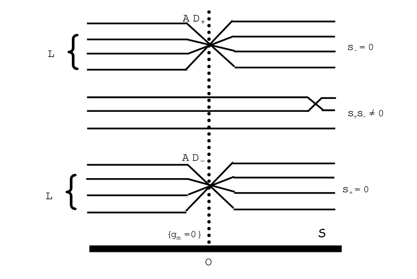
Figure 1: Features of the ${\cal N}=1$ vacuum bundle around the ${\cal N}=1$ $AD$ points:   The thick line at the bottom depicts the coupling constant space ${\cal S}$. The $AD_{+}$, $AD_{-}$ branches are characterized by $s_{-}=0$, $s_{+}=0$ respectively. $AD_{\pm}$ points are on the fiber over (dotted line) the origin $O$ of ${\cal S}$ and are located at the $L$-fold ramification points. The remaining lines depict the branches with $s_{+}s_{-}\neq 0$.

which is exactly the AD point of $U(N)$ theory (with the highest criticality). As we approach the AD point at the origin $O\equiv\{g_{m}=0,\,({}^{\forall}m=0,\ldots,n-1)\}$ of the base space $\cal S$, the monopole condensations (3.11) all vanish and we expect to obtain a scale invariant theory (note that we have $n\geq N/2+1$). As we see in the next section, physical observables exhibit scaling behaviors around this point: thus we conjecture that it represents a new class of ${\cal N}=1$ superconformal field theory. The ${\cal N}=1$ AD singularity in this case is located at the point where $L$ different branches of $s_{-}=0$ vacua collide in the vacuum bundle. Let us call this AD type singularity as the $AD_{+}$ point. See Fig.1.

The analysis of the case (2) is completely parallel. The monomial superpotential (3.1) generates a solution

$$P_{N}(x)^{2}-4\Lambda^{2N}=x^{N}(x^{N}+4\Lambda^{N})~{},$$

$$H(x)_{N-n}=x^{N-n}~{},~{}~{}~{}f_{n-1}(x)=4\Lambda^{N}x^{2n-N}~{},$$ (3.13)

which we call as the $AD_{-}$ point. The vacuum bundle near the $AD_{-}$ point again becomes an $L$-fold branched cover, and it defines a different branch from that of $AD_{+}$.

The case (3), on the other hand, is rather difficult to analyze. Even with a monomial superpotential we may obtain solutions of factorization equation which does not develop any singularities at $x=0$.

As a simple example, we have found the following solution in the case of $N=5$, $n=3$ with $s_{+}=s_{-}=1$ (although it is outside of the range of $n$ in (3.1));

$$P_{5}(x)+2\Lambda^{5}=\left(x+4^{1/5}\Lambda(1+\omega)\right)^{2}\left(x^{3}-4^{1/5}\Lambda x^{2}+4^{2/5}\Lambda^{2}(1+\omega)x-4^{3/5}\Lambda^{3}\omega\right)~{},$$

$$P_{5}(x)-2\Lambda^{5}=\left(x+4^{1/5}\Lambda\omega\right)^{2}\left(x^{3}+4^{1/5}\Lambda x^{2}-4^{2/5}\Lambda^{2}\omega x-4^{3/5}\Lambda^{3}(1+\omega)\right)~{},$$

$$P_{5}(x)^{2}-4\Lambda^{10}=\left(x+4^{1/5}\Lambda(1+\omega)\right)^{2}\left(x+4^{1/5}\Lambda\omega\right)^{2}\left\{W^{\prime}(x)^{2}+f(x)\right\}~{},$$

$$W^{\prime}(x)^{2}+f(x)=x^{6}+2\cdot 4^{4/5}\Lambda^{4}x^{2}+4\Lambda^{5}(-i\sqrt{3})x-4\cdot 4^{1/5}\Lambda^{6}~{},$$ (3.14)

where $\omega$ is the 3rd root of unity $\omega\equiv e^{2\pi i/3}$. Solutions of this kind do not correspond to any IR fixed point. Due to algebraic complexities we have not yet been able to study the case (3) in detail.

It seems, however, what happens is the following: by adjusting parameters it is possible to generate higher order zeros of the function, for instance, $P_{N}(x)+2\Lambda^{N}$ at some point $x=p_{i}$. At this point, however, $P_{N}(x)-2\Lambda^{N}$ can not vanish and thus the system is effectively reduced to the case of $s_{-}=0$ with the rank $N$ replaced by some smaller value. Thus the ${\cal N}=1$ AD points which appear on branches with $s_{+}s_{-}\not=0$ should be of the same type as those of $AD_{\pm}$ with lower rank gauge group.

It is worthwhile to note that when $n=N-1$, the case (3) does not occur and hence all the ${\cal N}=1$ vacua of the $U(N)$ gauge theory with an arbitrary degree-$N$ superpotential $W(x)$ are smoothly connected to the $AD_{\pm}$ points.

3.2 Non-zero Flavor

We next consider the system with non-zero flavors $N_{f}\neq 0$ (i.e. with $N_{f}$ chiral fields $Q_{i},\,\tilde{Q}_{i},\,i=1,\dots,N_{f}$ in the fundamental and anti-fundamental representations). For the sake of simplicity we consider the even flavor case $N_{f}=2\ell$, and discuss the case of degenerate bare masses $\{m_{i}=m,\,i=1,\dots,N_{f}\}$ in order to study higher singular points. It is convenient to make a constant shift of $\mbox{Tr}\,\Phi$, so that we can set $m=0$ without loss of generality. The SW curve is then written as [40]

$$y_{N=2}^{2}=C(x)^{2}-4\Lambda^{2(N-\ell)}x^{2\ell}~{},$$ (3.15)

where $C(x)$ is a degree $N$ polynomial of the form $C(x)=P_{N}(x)+{\cal O}(x^{N_{f}-N})$ ($C(x)=P_{N}(x)$, in the range $N_{f}<N$).

Now the higher singularities are achieved by the following steps:

1. Choose the moduli parameters so that the curve (3.15) possesses the maximal number of massless squarks (“highest non-baryonic branch” [41]). In other words we require the factorization

   $$y_{N=2}^{2}=x^{2\ell}\left(\tilde{C}(x)^{2}-4\Lambda^{2\tilde{N}}\right)~{},$$ (3.16)

   where we have introduced $\tilde{N}=N-\ell$ and $\tilde{C}(x)$ is of degree $\tilde{N}$. Physically this means that the Higgsing by the condensation of massless squarks breaks the gauge symmetry down to $U(\tilde{N})$.

2. We then tune the parameters in $\tilde{C}(x)$ so that the “reduced curve” $\tilde{y}_{N=2}^{2}=\tilde{C}(x)^{2}-4\Lambda^{2\tilde{N}}$ describing the Coulomb branch of $U(\tilde{N})$ theory possesses the higher critical points $\tilde{y}^{2}\approx x^{p}$, which is called the “class 4 model” in [29]. We especially focus on the case of highest criticality $p=\tilde{N}$, which is described by the curve

   $$y_{N=2}^{2}=x^{\tilde{N}+2\ell}\left(x^{\tilde{N}}-4\Lambda^{\tilde{N}}\right)~{}.$$ (3.17)

   $$(\mbox{or}~{}~{}y_{N=2}^{2}=x^{\tilde{N}+2\ell}\left(x^{\tilde{N}}+4\Lambda^{\tilde{N}}\right).)$$

It is obvious that we can work out the similar analysis as in the previous subsection by replacing $N$ with $\tilde{N}$. After turning on the monomial superpotential in the range of $n$

$$\frac{\tilde{N}}{2}+1\leq n\leq\tilde{N}-1~{},$$ (3.18)

we obtain the ${\cal N}=1$ AD points which reproduce the SW curve (3.17). The vacuum bundle around this point is again an $L$-fold branched covering space with $\displaystyle L={}_{n}C_{\tilde{N}-n}$. We can readily confirm that the squark condensation vanishes at this point

$$\left\langle\tilde{Q}_{\tilde{f}}Q^{f}\right\rangle=\mbox{const}\times y_{N=1}(x=-m=0)=0~{},~{}~{}~{}({}^{\forall}f,\tilde{f})~{},$$ (3.19)

using the formulas presented in [12, 14].

4 Scaling Behaviors Around the ${\cal N}=1$ AD Points

For the sake of simplicity we first consider the case of pure Yang-Mills theory. We introduce the monomial superpotential $W^{\prime}(x)=x^{n}$  and focus on the $AD_{+}$ point (3.12). The pair of relevant curves is given by

$$\Sigma_{N=2}:~{}y_{N=2}^{2}=x^{N}(x^{N}-4\Lambda^{N})~{},$$

$$\Sigma_{N=1}:~{}y_{N=1}^{2}=x^{2n-N}(x^{N}-4\Lambda^{N})~{}.$$ (4.1)

Our task is to evaluate the scaling behavior of the observables under the small perturbation

$$W^{\prime}(x)=x^{n}+\sum_{m=0}^{n-1}g_{m}\Lambda^{n-m}x^{m}~{},~{}~{}~{}|g_{m}|\ll 1~{}.$$ (4.2)

We can again apply the same scaling analysis given in section 2 and find

$$U_{r}(\{\rho^{\Delta(g_{m})}g_{m}\})\approx\rho^{\gamma(N+2r)}U_{r}(\{g_{m}\})~{},$$ (4.3)

$$S_{r}(\{\rho^{\Delta(g_{m})}g_{m}\})\approx\rho^{\gamma\left\{2(n+r+1)-N\right\}}S_{r}(\{g_{m}\})~{},$$ (4.4)

where we set the scaling dimensions of the coupling constants as

$$\Delta(g_{m})=2\gamma(n-m)~{},~{}~{}~{}(i=0,\ldots,m-1)~{}.$$ (4.5)

$\gamma$ is a positive real constant to be determined below.

Scaling analysis fixes the ratios of the scaling dimensions of coupling constants and physical observables, but cannot determine the overall normalization constant $\gamma$. To fix it, we demand that the effective superpotential $\displaystyle W_{\mbox{\scriptsize eff}}\equiv\langle\mbox{Tr}\,W(\Phi)\rangle$ should be a marginal operator at the AD point. This requirement amounts to $\Delta(U_{n+1})=3$, which implies $\gamma=3/(N+2n+2)$. In this way we arrive at the following formulas for scaling dimensions

$$\Delta(g_{m})=\frac{6(n-m)}{N+2n+2},\hskip 8.53581pt\Delta(U_{r})=\frac{3(N+2r)}{N+2n+2},\hskip 8.53581pt\Delta(S_{r})=\frac{3\big{(}2n-N+2(r+1)\big{)}}{N+2n+2}.$$ (4.6)

We note that

$$W_{\mbox{\scriptsize eff}}=\sum_{m=0}^{n}g_{m}U_{m+1},\hskip 11.38109pt\Delta(g_{m})+\Delta(U_{m+1})=3,\hskip 14.22636pt(g_{n}=1).$$ (4.7)

A general chiral perturbation to the $SCFT_{4}$ describing the ${\cal N}=1$ AD point is then given by

$$\Delta S=\int d^{4}xd^{2}\theta\,\sum_{m}g_{m}{\cal O}_{m}~{},\hskip 14.22636pt\left\langle{\cal O}_{m}\right\rangle=U_{m+1}$$ (4.8)

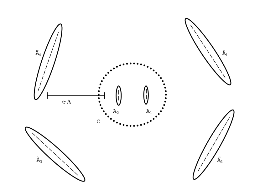
Figure 2: Cycles on the ${\cal N}=1$ curve near the AD point in the case $N=8$, $n=6$:   The broken lines depict the cuts. The “long cycles” $\tilde{A}_{i}$ correspond to the zeros of $H_{N-n}(x)^{2}F_{2n-N}(x)-4\Lambda^{2N}$, while the “short cycles” $A_{i}$ correspond to the zeros of $F_{2n-N}(x)$. Latter cycles are relevant for the IR physics. The dotted circle $C$ defines the chiral operators in the strong coupling ${\cal N}=1$ $SCFT_{4}$ by its contour integral.

The deformation (4.2) resolves the singularity at $x=0$, creating new cuts inside the circle $C$. See Fig.2. These cuts come from the zeroes of $F_{2n-N}(x)$ in the decomposition (3.5) and these are paired up to form $n-N/2$ new “$A$-cycles” on $\Sigma_{N=1}$. We denote them as $A_{i}$ $(i=1,\ldots,n-N/2)$. These cycles together with $\tilde{A}_{j}$ $(j=1,\ldots,N/2)$ compose the totality of $n$ $A$-cycles on $\Sigma_{N=1}$. The cycles $\tilde{A}_{i}$ and $A_{i}$ are separated by the length scale $\Lambda$ and describe the physics of different energy scales. Additional order parameters for the IR dynamics may be given by the integrals of $T(x)$ and $R(x)$ along $A_{i}$ (and corresponding $B$-cycles) as well as $C$ already introduced.

We can show that even with a perturbed superpotential (4.2)

$$\oint_{A_{i}}T(x)dx=0~{},~{}~{}~{}({}^{\forall}i=1,\ldots,n-N/2)~{},$$ (4.9)

thus

$$U_{0}=0.$$ (4.10)

It is easy to generalize our analysis to the non-zero flavor case (3.17) by replacing the color $N$ with $\tilde{N}\equiv N-\ell$. The non-trivial point is the existence of another chiral operator $M(x)^{f}_{\tilde{f}}=\left\langle\tilde{Q}_{\tilde{f}}(x-\Phi)^{-1}Q^{f}\right\rangle$. However, in this case we can readily find that

$$\oint_{C}x^{r}M(x)^{f}_{\tilde{f}}dx=\delta^{f}_{\tilde{f}}\oint_{C}x^{r-1}\left(R(x)-R(0)\right)dx~{},$$ (4.11)

based on the formulas given in [12, 14]. We thus need not introduce new observables describing scaling properties. We also point out the obvious relation

$$T(x)=\tilde{T}(x)+\frac{\ell}{x}~{},$$ (4.12)

where $\tilde{T}(x)$ is the counterpart of $T(x)$ for the pure gauge $U(\tilde{N})$ theory corresponding to the curve $\tilde{y}_{N=2}^{2}=\tilde{C}(x)^{2}-4\Lambda^{2\tilde{N}}$ defined in the factorization relation (3.16). The scaling formulas (4.6) likewise hold with replacing $N$ by $\tilde{N}$.

5 Summary and Comments

In this paper we have proposed a new class of IR fixed points with ${\cal N}=1$ supersymmetry which occur in a theory with a monomial superpotential $W^{\prime}(x)=x^{n},\,N/2+1\leq n\leq N-1$. They are located at the ramification points in the vacuum bundle over the coupling constant space and have been obtained by solving $s_{-}=0$ or $s_{+}=0$ branches of the factorization equation. Turning on small perturbations, we have analyzed the scaling behaviors of chiral ring operators. Our results strongly suggest that these ${\cal N}=1$ AD points define a new universality classes of ${\cal N}=1$ $SCFT_{4}$.

We have also studied the ${\cal N}=2$ AD points of $A_{N-1}$ type and confirmed the consistency with the approach of superstring theory compactified on the singular CY 3-folds and described by an ${\cal N}=2$ minimal model coupled to the ${\cal N}=2$ Liouville theory [32, 36]. In particular we have found that higher power chiral operators in the gauge theory side are identified with the gravitational descendants in the Liouville theory. We have found some evidence of the structure of the underlying $N$-reduced KP hierarchy in this system.

Finally we would like to present several comments:

1. One might suppose that the tree level superpotential $W(x)\approx x^{n+1}$ with higher values of $n$ could not affect the physics of IR region, since the naive power counting tells us that it is an irrelevant operator in the IR. One thus might guess that our ${\cal N}=1$ AD points belongs to the same universality class as the usual ${\cal N}=2$ AD points. However, as emphasized in [43], these superpotentials are the dangerously irrelevant operators in the theory of renormalization group. They behave as irrelevant operators around the UV fixed point (Gaussian fixed point), but do not necessarily around the IR fixed point when they could gain large anomalous dimensions due to the strong quantum effects. They could modify the IR physics and generate a new universality class. Our scaling analysis actually suggests this is indeed the case: The ${\cal N}=1$ AD points belong to the different universality classes from the ${\cal N}=2$ one (note that the dimension of the operator $\mbox{Tr}\,\Phi^{n+1}$ is equal $\frac{N+2(n+1)}{N+2}$ (2.19) at the ${\cal N}=2$ AD point, which is less than 3 when $\frac{N}{2}+1\leq n\leq N-1$, and thus it is a relevant perturbation).

2. We have observed that, when parameters are adjusted near the AD points, fluxes are localized on the large cycles of order $\Lambda$ and hence move out to infinity under the IR limit $\Lambda\,\rightarrow\,\infty$. This fact is essential for the appearance of non-trivial $SCFT_{4}$. Moreover, in the ${\cal N}=2$ case $W^{\prime}(x)=P_{N}(x)$, this phenomenon gives the theoretical justification why we can describe the AD points based on the superstring compactified on the singular $CY_{3}$ without flux.

3. It may be worthwhile to point out the similarity of our analysis to that of the topological Landau-Ginzburg models coupled with two-dimensional gravity [37, 38]. The approaches from the integrable hierarchy [44, 45, 46] is presumably useful in order to uncover the precise relation among these models. It is also interesting to look for the string theory description for the general ${\cal N}=1$ AD points as in the case of ${\cal N}=2$ points.

4. We have defined the ${\cal N}=1$ AD points by requiring that both of the Riemann surfaces $(\Sigma_{N=2},\Sigma_{N=1})$ develop higher isolated singularities at the same point. If the point $x=0$ is a singular point on $\Sigma_{N=2}$, but smooth on $\Sigma_{N=1}$, no interesting IR physics will be obtained. According to the formula (3.10), monopole condensation persists if $y_{N=1}\not=0$ at $x=0$ and we will be led to the confinement and mass gap. As is well-known that for ${\cal N}=2$ AD points one needs $y_{N=2}^{2}\approx x^{p},\,\,p\geq 3$ around the singularity $x=0$. We have imposed in this paper a condition $y_{N=1}^{2}\approx x^{q},\,\,q\geq 2$. In the exceptional case $y_{N=1}^{2}\approx x$ (where $\Sigma_{N=1}$ has no singularity), we still have a gap-less theory. However, it is easily found that all the VEV’s of chiral operators vanish even under the perturbed superpotential (4.2).

Note added : After the completion of this work we became aware of the papers [47, 48, 49], in which ${\cal N}=1$ extensions of Argyres-Douglas superconformal theory have also been discussed. We would like to thank S. Terashima, A. Gorsky and K. Konishi for bringing our attention to these references.

References

- [1] R. Dijkgraaf and C. Vafa, Nucl. Phys. B 644, 3 (2002) [arXiv:hep-th/0206255].
- [2] R. Dijkgraaf and C. Vafa, Nucl. Phys. B 644, 21 (2002) [arXiv:hep-th/0207106].
- [3] R. Dijkgraaf and C. Vafa, arXiv:hep-th/0208048.
- [4] C. Vafa, J. Math. Phys. 42, 2798 (2001) [arXiv:hep-th/0008142].
- [5] F. Cachazo, K. A. Intriligator and C. Vafa, Nucl. Phys. B 603, 3 (2001) [arXiv:hep-th/0103067].
- [6] F. Cachazo and C. Vafa, arXiv:hep-th/0206017.
- [7] R. Gopakumar and C. Vafa, Adv. Theor. Math. Phys. 3, 1415 (1999) [arXiv:hep-th/9811131].
- [8] H. Ooguri and C. Vafa, Nucl. Phys. B 577, 419 (2000) [arXiv:hep-th/9912123].
- [9] H. Ooguri and C. Vafa, Nucl. Phys. B 641, 3 (2002) [arXiv:hep-th/0205297].
- [10] R. Dijkgraaf, M. T. Grisaru, C. S. Lam, C. Vafa and D. Zanon, arXiv:hep-th/0211017.
- [11] F. Cachazo, M. R. Douglas, N. Seiberg and E. Witten, JHEP 0212, 071 (2002) [arXiv:hep-th/0211170].
- [12] N. Seiberg, JHEP 0301, 061 (2003) [arXiv:hep-th/0212225].
- [13] F. Cachazo, N. Seiberg and E. Witten, JHEP 0302, 042 (2003) [arXiv:hep-th/0301006].
- [14] F. Cachazo, N. Seiberg and E. Witten, arXiv:hep-th/0303207.
- [15] K. Konishi, Phys. Lett. B 135, 439 (1984). K. Konishi and K. Shizuya, Nuovo Cim. A 90, 111 (1985).
- [16] B. Feng, arXiv:hep-th/0212274.
- [17] C. Ahn and Y. Ookouchi, JHEP 0303, 010 (2003) [arXiv:hep-th/0302150].
- [18] E. Witten, arXiv:hep-th/0302194.
- [19] A. Brandhuber, H. Ita, H. Nieder, Y. Oz and C. Romelsberger, arXiv:hep-th/0303001.
- [20] V. Balasubramanian, B. Feng, M. x. Huang and A. Naqvi, arXiv:hep-th/0303065.
- [21] S. G. Naculich, H. J. Schnitzer and N. Wyllard, arXiv:hep-th/0303268.
- [22] L. F. Alday and M. Cirafici, arXiv:hep-th/0304119.
- [23] R. Casero and E. Trincherini, arXiv:hep-th/0304123.
- [24] P. Kraus, A. V. Ryzhov and M. Shigemori, arXiv:hep-th/0304138.
- [25] N. Seiberg and E. Witten, Nucl. Phys. B 426, 19 (1994) [Erratum-ibid. B 430, 485 (1994)] [arXiv:hep-th/9407087]; N. Seiberg and E. Witten, Nucl. Phys. B 431, 484 (1994) [arXiv:hep-th/9408099].
- [26] F. Ferrari, Phys. Rev. D 67, 085013 (2003) [arXiv:hep-th/0211069]; Phys. Lett. B 557, 290 (2003) [arXiv:hep-th/0301157].
- [27] P. C. Argyres and M. R. Douglas, Nucl. Phys. B 448, 93 (1995) [arXiv:hep-th/9505062].
- [28] P. C. Argyres, M. Ronen Plesser, N. Seiberg and E. Witten, Nucl. Phys. B 461, 71 (1996) [arXiv:hep-th/9511154].
- [29] T. Eguchi, K. Hori, K. Ito and S. K. Yang, Nucl. Phys. B 471, 430 (1996) [arXiv:hep-th/9603002].
- [30] S. Gukov, C. Vafa and E. Witten, Nucl. Phys. B 584, 69 (2000) [Erratum-ibid. B 608, 477 (2001)] [arXiv:hep-th/9906070].
- [31] A. D. Shapere and C. Vafa, arXiv:hep-th/9910182.
- [32] A. Giveon, D. Kutasov and O. Pelc, JHEP 9910, 035 (1999) [arXiv:hep-th/9907178].
- [33] S. Kharchev, A. Marshakov, A. Mironov, A. Morozov and A. Zabrodin, Phys. Lett. B 275, 311 (1992) [arXiv:hep-th/9111037]; S. Kharchev, A. Marshakov, A. Mironov, A. Morozov and A. Zabrodin, Nucl. Phys. B 380, 181 (1992) [arXiv:hep-th/9201013]; S. Kharchev, A. Marshakov, A. Mironov and A. Morozov, Nucl. Phys. B 397, 339 (1993) [arXiv:hep-th/9203043]; S. Kharchev, A. Marshakov, A. Mironov and A. Morozov, Mod. Phys. Lett. A 8, 1047 (1993) [Theor. Math. Phys. 95, 571 (1993 TMFZA,95,280-292.1993)] [arXiv:hep-th/9208046].
- [34] O. Pelc, JHEP 0003, 012 (2000) [arXiv:hep-th/0001054].
- [35] N. Seiberg, Prog. Theor. Phys. Suppl. 102, 319 (1990). D. Kutasov and N. Seiberg, Nucl. Phys. B 358, 600 (1991).
- [36] T. Eguchi and Y. Sugawara, Nucl. Phys. B 598, 467 (2001) [arXiv:hep-th/0011148].
- [37] A. Losev, Theor. Math. Phys. 95, 595 (1993) [Teor. Mat. Fiz. 95, 307 (1993)] [arXiv:hep-th/9211090].
- [38] T. Eguchi, H. Kanno, Y. Yamada and S. K. Yang, Phys. Lett. B 305, 235 (1993) [arXiv:hep-th/9302048]; T. Eguchi, Y. Yamada and S. K. Yang, Mod. Phys. Lett. A 8, 1627 (1993) [arXiv:hep-th/9304121].
- [39] J. de Boer and Y. Oz, Nucl. Phys. B 511, 155 (1998) [arXiv:hep-th/9708044].
- [40] A. Hanany and Y. Oz, Nucl. Phys. B 452, 283 (1995) [arXiv:hep-th/9505075]; P. C. Argyres, M. R. Plesser and A. D. Shapere, Phys. Rev. Lett. 75, 1699 (1995) [arXiv:hep-th/9505100]; J. A. Minahan and D. Nemeschansky, Nucl. Phys. B 464, 3 (1996) [arXiv:hep-th/9507032]; I. M. Krichever and D. H. Phong, J. Diff. Geom. 45, 349 (1997) [arXiv:hep-th/9604199].
- [41] P. C. Argyres, M. Ronen Plesser and N. Seiberg, Nucl. Phys. B 471, 159 (1996) [arXiv:hep-th/9603042].
- [42] S. G. Naculich, H. J. Schnitzer and N. Wyllard, JHEP 0301, 015 (2003) [arXiv:hep-th/0211254].
- [43] D. Kutasov, A. Schwimmer and N. Seiberg, Nucl. Phys. B 459, 455 (1996) [arXiv:hep-th/9510222].
- [44] L. Chekhov and A. Mironov, Phys. Lett. B 552, 293 (2003) [arXiv:hep-th/0209085].
- [45] L. Chekhov, A. Marshakov, A. Mironov and D. Vasiliev, arXiv:hep-th/0301071.
- [46] H. Itoyama and A. Morozov, Phys. Lett. B 555, 287 (2003) [arXiv:hep-th/0211259]; arXiv:hep-th/0301136.
- [47] S. Terashima and S. K. Yang, Phys. Lett. B 391, 107 (1997) [arXiv:hep-th/9607151]; Nucl. Phys. B 519, 453 (1998) [arXiv:hep-th/9706076].
- [48] A. Gorsky, A. I. Vainshtein and A. Yung, Nucl. Phys. B 584, 197 (2000) [arXiv:hep-th/0004087].
- [49] R. Auzzi, R. Grena and K. Konishi, Nucl. Phys. B 653, 204 (2003) [arXiv:hep-th/0211282].