TAUP-2725-03 hep-th/0305049

Probing Flavored Mesons of Confining Gauge Theories
by Supergravity

Tadakatsu Sakai and Jacob Sonnenschein

Raymond and Beverly Sackler Faculty of Exact Sciences
School of Physics and Astronomy
Tel-Aviv University , Ramat-Aviv 69978, Israel

We incorporate massive flavored fundamental quarks in the supergravity dual of ${\cal N}=1$ SYM by introducing D7 brane probes to the Klebanov Strassler background. We find probe configurations that solve the D7 equations of motion. We compute the quadratic fluctuations of the D7 brane and extract the spectrum of vector and pseudo scalar flavored mesons. The spectra found are discrete and exhibit a mass gap of the order of the glueball mass.

May 2003

1 Introduction

In the search for a supergravity model dual to a “realistic” strong coupling gauge dynamics (for a review see [1]), one should be able to incorporate quarks in the fundamental representation of an $SU(N_{c})$ gauge theory. Most of the known supergravity backgrounds duals of confining four dimensional gauge theories either do not incorporate quarks at all or admit quarks in the adjoint rather than the fundamental representation .

Since the early days of strings it has been understood that fundamental quarks should correspond to open strings. In the modern era of closed string theory this obviously calls for D branes. Certain basic objects of gauge theories like baryons [2], instantons, monopoles, domain walls[3] and others [4] were shown to correspond to wrapped D brane probes. It is thus natural to wonder, whether one can consistently add D brane probes to supergravity backgrounds duals of confining gauge theories, which will play the role of fundamental quarks. In case that $N_{f}$ the number of D brane probes is much smaller than $N_{c}$, one can convincingly argue that the backreaction of the probe on the bulk geometry is negligible.

It is well known that open strings between parallel $N_{f}$ D7 and $N_{c}$ D3 play the role of flavored quarks in the $SU(N_{c})$ gauge theory on the D3 4d world volume gauge theory. Karch and Katz [5] proposed to elevate this brane configuration into a supergravity background by introducing a D7 brane probe into the $AdS_{5}\times S^{5}$ background.

This idea was further explored in [6]. In [7] the spectrum of an ${\cal N}=2$ $SU(N_{c})$ SYM with fundamental hypermultiplet was extracted from the supergravity background of $AdS_{5}\times S^{5}$ with D7 brane probe . It was found that for massive quarks the spectrum was discrete with a mass gap. They also analyzed the semiclassical rotating open strings attached to the D7 brane and discussed meson meson interaction. For a related work, see also [8]

The purpose of this paper is two folded: (i) to find a supergravity dual of a confining gauge theory with flavors and (ii) to compute the mass spectra of the pseudo and vector mesons made of the flavored quarks from the SUGRA background. The first goal was in fact proposed but not explicitly proven in [5] and as for the second goal recall that the computation in [7] involves ${\cal N}=2$ SQCD which is not a confining gauge theory. The main idea behind our work is to introduce D7 brane probes into the Klebanov Strassler (KS) [9] background (this idea was first given in [5]). We will see that this configuration yields an ${\cal N}=1~{}SU(N_{c})$ gauge theory with massive $N_{f}$ flavors. The spectrum of the pseudo scalar and vector mesons can be extracted from the spectrum of scalar and vector fluctuations of the $N_{f}$ D7. It turns out that it is advantageous not to use the formulation of the deformed conifold of [10] but rather the coordinates introduced in [11]. In the latter picture there is a separation of the coordinates of the three manifold and the ${\bf S}^{2}$. It would be quite interesting to compare our results with a field theory analysis. We will leave it as a future problem.

To understand the construction of the probe D7 branes recall that in the type IIA T dual picture the singular locus of the conifold takes the form of a pair of perpendicular NS five branes [12, 13]. Once the conifold is deformed there will be a “diamond” structure at the intersection of the NS5 branes [14]. The fractional D3 branes of the KS model are mapped by the T duality to D4 branes connecting the two NS branes. Now in this type IIA configuration one adds D6 branes on top of the NS5 branes. The strings between the D6 and the D4 branes play the role of flavored fundamental quarks of the $SU(N)$ gauge theory[15]. T dualizing back to IIB the D6 branes get mapped into D7 branes that intersect the singular locus. The D7 branes in our configuration span the world volume coordinates of the D3 branes, the radial direction and wrap the three cycle of the deformed the conifold. The transverse coordinates are the coordinates of the ${\bf S}^{2}$ part of the base. In terms of the transverse coordinates this means having one D7 brane at the north pole and another in the south pole of the ${\bf S}^{2}$. These “two” D7 branes are in fact one D7 brane since they smoothly connect at the origin of the radial direction. By writing down the 8d effective action of the D7 branes which includes the DBI term and the WZ term, we have shown that indeed these D7 brane configurations are solutions of the equations of motion. As a consistency check, the probe configuration satisfies the RR-flux cancellation condition. We will see that the probe configuration admits the isometry $SU(2)\times U(1)$ which is the subgroup of the isometry group of the deformed conifold $SU(2)\times SU(2)$.

We then analyze the fluctuation modes around this classical D7 brane solution. The worldvolume theory of the D7 probe contains $U(N_{f})$ gauge fields as well as (pseudo) scalars in the adjoint of the non-abelian flavor group. Kaluza-Klein(KK) reduction of the fluctuations around the compact three manifold of the 8d scalars yields 5d (pseudo) scalars whereas the vector fields yield vectors as well as pseudo scalars. We then determine the quadratic fluctuations which are solutions of the equations of motion of the 5d effective action. Both type of fluctuations have quantum numbers that are compatible with those of pseudo scalar and vector mesons of ${\cal N}=1$ SQCD, namely they are in the adjoint of $SU(N_{f})$ and carry zero baryon number. To ensure that these modes are trivial under the $SU(2)\times U(1)$ global symmetry, we consider only a massless 5d vector fluctuation and the lowest scalar ones.

A crucial point in the extraction of the mesonic spectra from the corresponding fluctuations is that these are normalizable with an appropriate regularity condition satisfied at the origin of the deformed conifold. As a consequence, we show that the spectrum is discrete with a mass gap for the vector mesons. We also argue that the pseudo scalar meson spectrum exhibits the same behavior. It is shown that the system of mesons is stable (in the quadratic order approximation) since the kinetic term of the scalar fluctuations is positive and since there are no tachyonic masses. The mass scale of the mesons is that of the glueballs, namely, $M_{\rm meson}\sim{\epsilon^{2/3}\over g_{s}N\alpha^{\prime}}$.

The paper is organized as follows. In section 2, the KS background is described in the alternative formulation of [11]. The action of the D7 probe including the DBI part and the WZ is analyzed in section 3. We determine the solutions of the equations of motion that correspond to two D7 brane probes that merge smoothly into each other at the origin. Section 4 is devoted to the determination of the fluctuations around the probe configurations and the extraction of the mesonic spectrum. In subsection 4.1 the quadratic fluctuations are analyzed and then in subsections 4.2 and 4.3 the spectrum of the vector mesons and the scalar mesons is computed. We summarize and discuss some open questions in section 5. Some useful formulae are summarized in the appendix.

2 The KS model and the geometry of a deformed conifold

The KS background is based on adding fractional D3 branes into the deform conifold. The original KS metric [9]

$$ds_{10}^{2}=h^{-1/2}dx_{\mu}^{2}+h^{1/2}dx_{6}^{2},$$ (2.1)

made use of the metric of a deformed conifold given in [10]. It turns out that for our purposes it is more convenient to use the formulation of [11] since it admits a separation between the three cycle and two cycle of the deformed conifold. It is given by

$$\epsilon^{-4/3}ds_{6}^{2} \!=\! {1\over 4}\,K(\tau)\,\cosh(\tau)\,\left(d\tau^{2}+(\omega^{a})^{2}\right)$$ (2.2)

$$+K(\tau)\,\sinh^{2}({\tau\over 2})\;\Bigg{[}\;(d\theta^{2}+\sin^{2}\theta\,d\phi^{2})-(\sin\phi\,\omega^{1}+\cos\phi\,\omega^{2})(d\theta)$$

$$\qquad-\,(\cos\theta\cos\phi\,\omega^{1}-\cos\theta\sin\phi\,\omega^{2}-\sin\theta\,\omega^{3})(\sin\theta\,d\phi)\Bigg{]}$$

$$+{1\over 4}\,K^{\prime}(\tau)\,\sinh(\tau)\Big{[}\;d\tau^{2}\;+\;(\sin\theta\cos\phi\,\omega^{1}+\sin\theta\sin\phi\,\omega^{2}+\cos\theta\,\omega^{3})^{2}\Big{]}.$$

Here

$$K(\tau)={(\sinh(2\tau)-2\tau)^{1/3}\over 2^{1/3}\sinh\tau},~{}~{}h(\tau)=(g_{s}M\alpha^{\prime})^{2}\,2^{2/3}\,\epsilon^{-8/3}I(\tau),$$ (2.3)

$$I(\tau)=\int_{\tau}^{\infty}dx\,{x\coth x-1\over\sinh^{2}\!x}\left(\sinh(2x)-2x\right)^{1/3}.$$ (2.4)

For instance it is easy to verify in this formulation that for $\tau=0$, the 6d metric reduced to $\sum(\omega^{a})^{2}$, giving the ${\bf S}^{3}$ while the ${\bf S}^{2}$ shrinks to zero.

It is useful to rewrite the metric as follows

$$ds_{10}^{2}=R^{2}\left(m^{2}I^{-1/2}dx_{\mu}^{2}+I^{1/2}d\tilde{x}_{6}^{2}\right),$$ (2.5)

where

$$R^{2}=2^{1/3}g_{s}M\alpha^{\prime},~{}~{}m^{2}={\epsilon^{4/3}\over 2^{2/3}(g_{s}M\alpha^{\prime})^{2}},$$ (2.6)

and $\epsilon^{-4/3}ds_{6}^{2}=d\tilde{x}_{6}^{2}$. $m$ is the mass scale of glueballs. For a detail of the glueball spectrum in the KS background, see [16].

The NS B-field is

$$B_{2}={g_{s}M\alpha^{\prime}\over 2}\Big{[}(f+k)\,\widetilde{g}^{3}\wedge\widetilde{g}^{4}+\sqrt{2}k\,\widetilde{g}^{3}\wedge d\theta+\sqrt{2}k\,\widetilde{g}^{4}\wedge\sin\theta d\phi+2k\,\sin\theta d\theta\wedge d\phi\Big{]}.$$ (2.7)

Here

$$f(\tau) \!=\! {\tau\coth\tau-1\over 2\sinh\tau}\,(\cosh\tau-1)\ ,$$

$$k(\tau) \!=\! {\tau\coth\tau-1\over 2\sinh\tau}\,(\cosh\tau+1)\ .$$ (2.8)

For the definition of the one-forms $\widetilde{g}$, see the appendix. The RR 2-form potential reads

$$C_{2}={M\alpha^{\prime}\over 2}\left[{1\over 2}\cos\theta^{\prime}d\psi^{\prime}\wedge d\phi^{\prime}+\sqrt{2}F(\tau)\left(\widetilde{g}^{3}\wedge\sin\theta d\phi-\widetilde{g}^{4}\wedge d\theta\right)\right].$$ (2.9)

Here

$$F(\tau)={\sinh\tau-\tau\over 2\sinh\tau}\ .$$ (2.10)

We will later need the explicit expression for $C_{6}$ the RR six form. The corresponding RR 7-form field strength $F_{7}=dC_{6}$ is defined by

$$dF_{7}=d^{\ast}dC_{2}-F_{5}\wedge dB_{2}\ ,$$ (2.11)

where $F_{5}$ is the self-dual 5-form field strength given by

$$F_{5}={\cal F}_{5}+{}^{\ast}{\cal F}_{5}\ ,$$ (2.12)

with

$${\cal F}_{5} \!=\! B_{2}\wedge dC_{2}={gM^{2}\alpha^{\prime 2}\over 4}\,l(\tau)\,g^{1}\wedge g^{2}\wedge g^{3}\wedge g^{4}\wedge g^{5}\ ,$$

$${}^{\ast}{\cal F}_{5} \!=\! {\alpha\,l(\tau)\over g_{s}\,K^{2}h^{2}\sinh^{2}\!\tau}\,d^{4}x\wedge d\tau\ ,$$ (2.13)

with $\alpha=4(g_{s}M\alpha^{\prime})^{2}\epsilon^{-8/3}$ and

$$l(\tau)=f(1-F)+kF={\tau\coth\tau-1\over 4\sinh^{2}\!\tau}(\sinh 2\tau-2\tau)\ .$$ (2.14)

¿From the equation of motion of $C_{2}$ it follows that $dF_{7}=0$. We thus obtain

$$C_{6} \!=\! {M\alpha^{\prime}\over 4}(f^{\prime}+k^{\prime})h^{-1}d^{4}x\wedge d\tau\left(-\sin\theta\cos\phi\,\omega^{1}+\sin\theta\sin\phi\,\omega^{2}-2\cos\theta\,d\phi\right)$$ (2.15)

$$\!-\! {M\alpha^{\prime}\over 4}\,(k-f)h^{-1}\,d^{4}x\left[\sqrt{2}\left(\widetilde{g}^{3}\,d\theta+\widetilde{g}^{4}\sin\theta d\phi\right)+2\sin\theta d\theta d\phi\right]\ .$$

where ${}^{\prime}=\partial/\partial\tau$. Finally we notice that the RR-4-form gauge potential is defined by

$$F_{5}=dC_{4}+B_{2}\wedge dC_{2}=B_{2}\wedge dC_{2}+{}^{\ast}(B_{2}\wedge dC_{2})\ ,$$ (2.16)

from which we obtain

$$C_{4}={2^{4/3}(mR)^{4}\over g_{s}}\,u(\tau)\,d^{4}x\ .$$ (2.17)

Here $u(\tau)$ is defined by

$$u^{\prime}(\tau)={l(\tau)\over K^{2}I^{2}\sinh^{2}\!\tau}\ .$$ (2.18)

Let us now review briefly some geometrical aspects of the deformed conifold. The deformed conifold is defined by

$$w_{1}w_{2}-w_{3}w_{4}=-{\epsilon^{2}\over 2}\ .$$ (2.19)

For the explicit form of $w_{i}$, see the appendix. This can be regarded as a ${\bf C}^{\ast}$ fibration over a two-dimensional complex plane spanned by $w_{3},w_{4}$. The fibers get degenerate when $w_{1}w_{2}=0$, giving a smooth singular locus in the base which is T-dual to an NS5-brane [12]. It turns out that the condition $w_{1}w_{2}=0$ can be solved as (1) $\theta=0,~{}\theta^{\prime}=\pi$, (2) $\theta=\pi,~{}\theta^{\prime}=\pi$. Each corresponds to a cylinder that intersect with one another at a circle. To see this, note that for the two cases one finds

$$w_{1}=w_{2}=0,$$

$$w_{3}={i\epsilon\over\sqrt{2}}e^{{i\over 2}(\phi^{\prime}-\psi^{\prime})}\left(\pm\sinh{\tau\over 2}-\cosh{\tau\over 2}\right),$$

$$w_{4}={i\epsilon\over\sqrt{2}}e^{-{i\over 2}(\phi^{\prime}-\psi^{\prime})}\left(\pm\sinh{\tau\over 2}+\cosh{\tau\over 2}\right).$$ (2.20)

These denote two cylinders spanned by $\tau,\phi^{\prime}-\psi^{\prime}$ that intersect with each other at a circle at $\tau=0$. Recall that the circle is embedded in the ${\bf S}^{3}$ and has a radius proportional to $\epsilon$. This circle corresponds to a diamond [14]. In the limit $\epsilon\rightarrow 0$ where the deformed conifold reduces to a conifold, the radius goes to zero so that the smooth locus is split into two separate cones that intersect with each other at the tips of the cones. The T-dual of the conifold [13] gives us the IIA brane configuration that consists of two perpendicular NS5 branes, one at $w_{1}=0$ and the other at $w_{2}=0$.

3 The D7 brane probes in the KS background

Now let us consider D7 probes in the KS background that yield massive flavors, which were first discussed in [5]. For that purpose, it is useful to start from the T-dualized picture of the conifold limit $\epsilon\rightarrow 0$. The fractional D3-branes get mapped to D4-branes extending to the cycle. In this setup, one can add D6-branes on top of either of the two perpendicular NS5-branes to get ${\cal N}=1$ SQCD with massless flavors [17], because the D4-branes divide the D6-branes into two pieces, each of which is responsible for chiral flavor groups. Upon T-dualizing the IIA brane configuration back, each type of D6-branes gets mapped to different D7-branes [18]: one is D7-branes which intersect with the singular locus $w_{1}=0$ and the other D7-branes intersect with $w_{2}=0$.

Now turn on $\epsilon\neq 0$ to have the deformed conifold. As seen before, the singular loci become a single smooth cylinder. Correspondingly, the two kinds of D7-branes intersecting the singular loci become a smooth component of D7-branes that intersects with the smooth locus. More precisely, let us define D7₍₁₎-branes staying at $\theta=0$, the north pole of the ${\bf S}^{2}$ and D7₍₂₎-branes staying at $\theta=\pi$, the south pole of the ${\bf S}^{2}$. See figure 1.

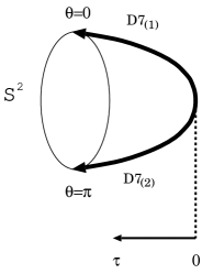
Figure 1: Configuration of 7-branes on 2-sphere

We show that these two seven branes intersect with each other at the ${\bf S}^{3}$ at $\tau=0$ and form a smooth D7-brane: we first notice that the world volumes of the D7₍₁₎ and D7₍₂₎ are charactorized by

$$w_{1,2}^{(1)} \!=\! {\epsilon\over\sqrt{2}}\,\cos{\theta^{\prime}\over 2}\,e^{\pm{i\over 2}(\phi^{\prime}+\psi^{\prime})}\left(\sinh{\tau\over 2}\pm\cosh{\tau\over 2}\right)\ ,$$

$$w_{3,4}^{(1)} \!=\! {i\epsilon\over\sqrt{2}}\,\sin{\theta^{\prime}\over 2}\,e^{\pm{i\over 2}(\phi^{\prime}-\psi^{\prime})}\left(\sinh{\tau\over 2}\mp\cosh{\tau\over 2}\right)\ ,$$ (3.1)

and

$$w_{1,2}^{(2)} \!=\! {\epsilon\over\sqrt{2}}\,\cos{\theta^{\prime}\over 2}\,e^{\pm{i\over 2}(\phi^{\prime}+\psi^{\prime})}\left(-\sinh{\tau\over 2}\pm\cosh{\tau\over 2}\right)\ ,$$

$$w_{3,4}^{(2)} \!=\! {i\epsilon\over\sqrt{2}}\,\sin{\theta^{\prime}\over 2}\,e^{\pm{i\over 2}(\phi^{\prime}-\psi^{\prime})}\left(-\sinh{\tau\over 2}\mp\cosh{\tau\over 2}\right)\ .$$ (3.2)

It is easy to see that

$$\omega_{i}^{(1)}(\tau=0)=\omega_{i}^{(2)}(\tau=0)\ ,~{}~{}~{}\partial_{\tau}\omega_{i}^{(1)}(\tau=0)=-\partial_{\tau}\omega_{i}^{(2)}(\tau=0)\ .$$ (3.3)

These relations guarantee the smooth connection of the 7-branes at $\tau=0$.

Recall that in the deformed conifold the chiral flavor symmetry is broken to the diagonal subgroup $U(N_{f})$, as we are left with only a single type of D7-branes. This implies that turning on $\epsilon$ amounts to turning on a vev for a Higgs field on the 7-branes that transforms as the bifundamental representation of the chiral flavor group. This vev plays the role of a mass term in the 4d gauge theory on the fractional D3 branes.

Let us now analyze the D7-probe action in the KS background to verify that the configuration solves the equation of motion. The action consists of two parts

$$S=S_{\rm DBI}+S_{\rm WZ}\ ,$$ (3.4)

where

$$S_{\rm DBI} \!=\! -{\mu_{7}\over g_{s}}\int d^{8}\sigma\,\sqrt{-\det\left(\phi^{\ast}g+\phi^{\ast}B_{2}+2\pi\alpha^{\prime}F\right)}\ ,$$ (3.5)

$$S_{\rm WZ} \!=\! -\mu_{7}\int e^{2\pi\alpha^{\prime}F+B}\wedge\sum_{p}C_{p+1}$$ (3.6)

$$\!=\! -\mu_{7}\int\left({1\over 6}(2\pi\alpha^{\prime}F+B)^{3}C_{2}+{1\over 2}(2\pi\alpha^{\prime}F+B)^{2}C_{4}+(2\pi\alpha^{\prime}F+B)C_{6}\right)\ .$$

Here $\phi^{\ast}g,\phi^{\ast}B_{2}$ are the pull-backs of $g,B_{2}$. $F$ is the $U(1)$ field strength on the brane. $\mu_{7}=1/(2\pi)^{7}\alpha^{\prime 4}$. The two transverse coordinates of a probe D7 are taken to be $\theta,\phi$ while upon taking the static gauge the world volume coordinates are given by $X^{\alpha}=(X^{I},\theta^{\prime},\phi^{\prime},\psi^{\prime})$, with $X^{I}=(x^{\mu},\tau)$. What we should show is that the D7₍₁₎ given by $\theta=0,~{}{\rm any}~{}\phi$, and the D7₍₂₎ given by $\theta=\pi,~{}{\rm any}~{}\phi$ solve the equation of motion. In order to check first the D7₍₁₎ brane, we assume $\theta={\rm const},~{}\phi=\phi(X^{\alpha})$ and expand the action around $\theta=0$. It is verified that the coefficients of the linear term in $\theta$ depend linearly on some of the components of $F$. By requiring them to vanish, we find that the $U(1)$ gauge potential on the probe should take the form

$$A=A_{3}(\tau)\omega^{3}\ .$$ (3.7)

It is then not difficult to show that the action becomes

$$S_{\rm DBI} \!=\! -{\mu_{7}R^{8}\over g_{s}}\int d^{8}X\sqrt{-\det(g_{(8)}+R^{-2}B_{2}^{(0)})}$$

$$\quad\times\Bigg{[}\left(1+{4\over I^{1/2}(K\sinh\tau)^{\prime}}\,g^{\tau\tau}\partial_{\tau}\widetilde{A}_{3}\,\partial_{\tau}\widetilde{A}_{3}\right)\left(1-{8x\over I^{1/2}J}\widetilde{A}_{3}+{16\over IJ}\widetilde{A}_{3}^{2}\right)\Bigg{]}^{1/2}\Big{(}1+{\cal O}(\theta^{2})\Big{)}\ ,$$

$$S_{\rm WZ} \!=\! -{\mu_{7}R^{8}m^{4}\over 2^{4}g_{s}}\int d^{4}x\,d\tau\,\omega^{1}\omega^{2}\omega^{3}\,\Big{(}1+{\cal O}(\theta^{2})\Big{)}$$

$$\times\Bigg{[}2^{-2/3}(f+k)(f^{\prime}+k^{\prime})I^{-1}+\Big{(}2^{5/3}(f^{\prime}+k^{\prime})I^{-1}+2^{3}\,\partial_{\tau}((f+k)u)\Big{)}\,\widetilde{A}_{3}-2^{13/3}\,u^{\prime}\,\widetilde{A}_{3}^{2}\Bigg{]}\ .$$

Here $\widetilde{A}_{3}={2\pi\alpha^{\prime}\over R^{2}}A_{3}$ and

$$g_{(8)\alpha\beta}dX^{\alpha}dX^{\beta} \!=\! g_{IJ}dX^{I}dX^{J}+{I^{1/2}\over 4}\Big{(}K\cosh\tau\left((\omega^{1})^{2}+(\omega^{2})^{2}\right)+(K\sinh\tau)^{\prime}(\omega^{3})^{2}\Big{)}\ ,$$ (3.9)

$$R^{-2}B_{2}^{(0)} \!=\! -{f+k\over 2^{7/3}}\,\omega^{1}\wedge\omega^{2}\ ,$$ (3.10)

with

$$g_{IJ}dX^{I}dX^{J}=m^{2}I^{-1/2}dx_{\mu}^{2}+{I^{1/2}\over 4}\,(K\sinh\tau)^{\prime}\,d\tau^{2}\ .$$ (3.11)

Also

$$J=(K\cosh\tau)^{2}+x^{2}\ ,~{}~{}~{}x={f+k\over 2^{4/3}I^{1/2}}\ .$$ (3.12)

Since there appear no linear terms in $\theta$, we find that $\theta=0$ solves the equation of motion of $\theta$. However $A_{3}=0$ is not a solution because $A_{3}$ couples to a non-trivial current. We can easily see that the current is conserved. Recall that the contribution of the current from the DBI action is due to the non-trivial NS B-fields. The equation of motion of $A_{3}$ is so complicated that no explicit form of the solution is found. The solution must be given to evaluate the tension of the probe 7-brane. We leave it as an open problem. However, the D7₍₁₎ probe configuration itself is allowed as the existence of the solution to the equation of motion should be guaranteed. It is interesting that the gauge configuration induces a D3-brane charge on the probe:

$$\int F\wedge F=2\int d\tau\,\omega^{1}\omega^{2}\omega^{3}\,F_{\tau 3}F_{12}\ .$$ (3.13)

Also by expanding the action around $\theta=\pi$ with any $\phi$ and the same form of the $U(1)$ potential, we obtain the same form of the action as above. Hence the D7₍₂₎ probe also solves the equation of motion.

Recall that (3.9) gives the metric of the 8d hypersurface that denotes the embedding of the D7₍₁₎ and D7₍₂₎ probes in KS. We will refer to the compact 3d submanifold as $M_{3}$. $M_{3}$ is topologically ${\bf S}^{3}$ and admits the isometry group $SU(2)\times U(1)$, where $SU(2)$ is the left transformation of $T$ that leaves $\omega^{a}$ invariant and $U(1)$ is the subgroup of the right $SU(2)$ under which $\omega^{1,2}$ transform as a doublet while $\omega^{3}$ is invariant. One finds that the isometry group leaves $B_{2},C_{2},C_{4}$ and $A$ invariant as well.

Here it is crucial to notice that the solution satisfies the consistency condition of the RR-flux cancellation. ¿From the 10d point of view the two D7 branes carry opposite RR charges on ${\bf S}^{2}$ so that the total charge vanishes. See figure 1.

To summarize, the probe D7-brane configuration looks like figure 2.

Figure 2: D7-probe configuration in a deformed conifold. The vectors denote the singular locus where the elliptic fibers get degenerate. The two shadowed surfaces that intersect with each vector are the 7-brane probes.

4 Spectrum of mesons

In this section, we study the fluctuation modes around the D7 probe configuration. Since these belong to the adjoint representation of $U(N_{f})$, so do the dual states in the QCD. We thus expect to find the information about mesons made out of the fundamental quarks. Recall that no state in the adjoint of $U(N_{f})$ is charged under the baryon number $U_{B}(1)$, where $U(N_{f})=SU(N_{f})\times U_{B}(1)$. There exist two kinds of mesons we can learn about in the present context: pseudo-scalar and vector mesons. To see this, let us start with the D7 action defined on the probe configuration. We have two kinds of dynamical fields on it, 8d gauge potentials and 8d scalars that correspond to the fluctuation along the transverse directions. Upon KK reduction around $M_{3}$, we obtain an effective 5d theory that consists of the infinite number of 5d vector and 5d scalar fields. We see that the 5d vectors are dual to vector mesons in the dual QCD, and the 5d scalars dual to pseudo-scalar mesons. Here we consider only the lowest-lying KK modes, namely, a massless 5d vector and two 5d scalar fields, one coming from KK reduction of a 8d scalar by a scalar harmonics and the other from that of a 8d vector by a vector harmonics. The reason why we ignore the other massive modes is that these modes are irrelevant to the physics of QCD: since $M_{3}$ has the isometry $SU(2)\times U(1)$, the nontrivial harmonics carry non-zero spins and $U(1)$ charges. However there is no counterpart of these quantum numbers in the dual QCD.

In this section, we examine quadratic fluctuations of the D7 action with $N_{f}=1$ around the probe configuration and derive the effective 5d theory that involves only the lowest-lying KK modes. As far as our concern is in quadratic fluctuations, we can concentrate on the case $N_{f}=1$, since to this order any non-abelian interaction is irrelevant and consequently a field in the adjoint representation of $U(N_{f})$ reduces to $N_{f}^{2}$ free fields. Based on this, we perform a numerical computation of the spectrum of vector and scalar mesons. In fact these are pseudo scalars rather than scalars as follows from a straightforward parity analysis. Recall that the 8d super Yang-Mills(SYM) theory on a D7 comes from dimensional reduction of 10d SYM. In ten dimensions, the parity transformation for the 10d vector field is defined as

$${\cal P}A(t,\vec{x}_{9}){\cal P}^{-1}=-A(t,-\vec{x}_{9})\ .$$ (4.1)

Upon dimensional reduction to 8d, we find that the 8d scalar and vector fields have parity odd. Since the scalar and vector harmonics on $M_{3}$ have parity even, the 5d scalars and vectors have parity odd.

4.1 Quadratic perturbations around the probe configuration

Here we consider the fluctuation around the D7₍₁₎-branes in some detail. The analysis of the D7₍₂₎-brane is then straightforward. In fact, one ends up with the same results in the two cases.

As mentioned above, we assume

$$\theta=\theta(X^{I}),~{}~{}\phi=\phi(X^{I})\ .$$ (4.2)

The 8d scalars $\theta$ and $\phi$ reduce to the 5d scalars via a constant mode on $M_{3}$. The constant mode is the normalizable zero mode of the scalar harmonics as $M_{3}$ is compact. The 8d vector $A$ yields a 5d massless vector and a 5d scalar field. To see which vector harmonics is to be taken to obtain the 5d scalar, we first recall that the lowest-lying vector harmonics on ${\bf S}^{3}$ transform under the isometry $SU(2)\times SU(2)$ as $({\bf 3},{\bf 1})\oplus({\bf 1},{\bf 3})$. $M_{3}$ at hand is topologically ${\bf S}^{3}$ and admits as the isometry the subgroup $SU(2)\times U(1)$. The lowest-lying vector harmonics then splits into some of the vector harmonics on $M_{3}$ that belong to an irreducible representation of $SU(2)\times U(1)$, one of them being singlet. In fact, it is found that the singlet vector harmonics is given by $\omega^{3}$. We thus find that the the 5d scalar corresponds to the fluctuation of $A_{3}$ in (3.7) around the solution of the system (LABEL:Sprobe). However, since the solution is not known, one can not obtain the explicit form of the action that governs the fluctuation. As we will see below, up to quadratic order this fluctuation mode decouples from the other 5d scalar and vector modes. In this paper, we focus on only the two modes to compute the meson spectrum.

It turns out that up to quadratic terms in the fluctuations, the DBI action takes the form

$$S_{\rm DBI} \!=\! -{\mu_{7}R^{8}m^{4}\over 2^{4}\,g_{s}}\int d^{5}X\,\omega^{1}\omega^{2}\omega^{3}\,(K\sinh\tau)^{\prime}J^{1/2}$$ (4.3)

$$\times\Bigg{[}1+{L\over 2}\,g^{IJ}\partial_{I}\theta\partial_{J}\theta+{1\over 4}\left({2\pi\alpha^{\prime}\over R^{2}}\right)^{2}g^{IJ}g^{KL}F_{IK}F_{JL}$$

$$~{}~{}~{}~{}+\left({2\pi\alpha^{\prime}\over R^{2}}\right)^{2}\left({1\over 2}\,g^{IJ}u^{33}\,\partial_{I}A_{3}\,\partial_{J}A_{3}+{8(K\cosh\tau)^{2}\over IJ^{2}}\,A_{3}^{2}\right)-{2\pi\alpha^{\prime}\over R^{2}}\,{8x\over I^{1/2}J}A_{3}\Bigg{]}\ .$$

Here

$$L={K\cosh\tau\over 4I^{1/2}J}\left[IK^{2}\sinh^{2}\!\tau+{1\over 2^{8/3}}(\tau\coth\tau-1)^{2}\right]\ .$$ (4.4)

$a,b=1,2,3$ are the indices of the orthonormal frame of ${\bf S}^{3}$, see the appendix for detail. $u_{ab}$ is defined by the 3d part of the tensor $g_{(8)}+R^{-2}B_{2}^{(0)}$ and given by

$$u_{ab}={I^{1/2}\over 4}\left(\begin{array}[]{ccc}K\cosh\tau&-x&0\\ +x&K\cosh\tau&0\\ 0&0&(K\sinh\tau)^{\prime}\end{array}\right)\ .$$ (4.8)

On the other hand, we find that the fluctuations from the WZ term up to quadratic order are given by $S_{\rm WZ}$ in (LABEL:Sprobe). This shows that $\theta$ and $A_{I}$ have no mixing terms. As mentioned before, $A_{3}$ can not be diagonalized because one has to expand this around a non-trivial configuration that solves the action (LABEL:Sprobe).

It is interesting to notice that the kinetic term of $\theta$ is always positive. This implies the stability of the probe configuration at hand.

4.2 Vector mesons

Let us first study the 5d vector part to compute the vector meson spectrum. Part of the analysis given here is parallel to [19] that aimed at investigating a localization of a bulk gauge field at a brane world.

The action of the 5d gauge potential is

$$S_{\rm v}\sim m^{4}\int d^{5}X\,(K\sinh\tau)^{\prime}\,\sqrt{J}\,g^{IJ}g^{KL}F_{IK}F_{JL}.$$ (4.9)

Here we neglect the overall numerical factor because this is irrelevant for the purpose of computing the mass spectrum of mesons. The equation of motion reads

$$\partial_{J}\Big{(}(K\sinh\tau)^{\prime}\,\sqrt{J}\,g^{IJ}g^{KL}F_{IK}\Big{)}=0.$$ (4.10)

For the component $L=\tau$, this becomes

$$0=\eta^{\mu\nu}\partial_{\mu}(\partial_{\nu}A_{\tau}-\partial_{\tau}A_{\mu}).$$ (4.11)

It is useful to work in the gauge $A_{\tau}=0$. Then the above equation gives us the Gauss law constraint. We next decompose the rest components of the gauge potential in terms of the complete set of functions $\chi_{n}(\tau)$:

$$A_{\mu}(x,\tau)=\sum_{n}A_{\mu}^{(n)}(x)\chi_{n}(\tau).$$ (4.12)

$\chi$ satisfy a second-order differential equation we will present below. Note that we are interested in only normalizable solutions. Substituting the decomposition into the Gauss law constraint, we obtain

$$0=\sum_{n}\eta^{\mu\nu}\partial_{\mu}A_{\nu}^{(n)}(x)\,\partial_{\tau}\chi_{n}(\tau).$$ (4.13)

As we will see later, the constant mode is not normalizable so that we find

$$\eta^{\mu\nu}\partial_{\mu}A_{\nu}^{(n)}=0.$$ (4.14)

This implies that $A_{\mu}^{(n)}$ are Proca fields. Substituting (4.12) into the action, we obtain

$$S_{\rm v} \!=\! \int d^{4}x\,d\tau\,(K\sinh\tau)^{\prime}\,\sqrt{J}$$

$$\sum_{n,m}\Big{[}I\,\eta^{\mu\nu}\eta^{\rho\sigma}F_{\mu\rho}^{(n)}F_{\nu\sigma}^{(m)}\chi_{n}(\tau)\chi_{m}(\tau)+{8m^{2}\over(K\sinh\tau)^{\prime}}\,\eta^{\mu\nu}A_{\mu}^{(n)}A_{\nu}^{(m)}\,\partial_{\tau}\chi_{n}(\tau)\,\partial_{\tau}\chi_{m}(\tau)\Big{]}\ .$$

Now we define $\chi_{n}$ as the solution of the differential equation

$$-{1\over\sqrt{\gamma}}\,\partial_{\tau}\left({\sqrt{\gamma}\over(K\sinh\tau)^{\prime}\,I(\tau)}\,\partial_{\tau}\chi_{n}\right)=\lambda_{n}\,\chi_{n}(\tau),$$ (4.16)

with the normalization condition given by

$$\int_{0}^{\infty}d\tau\,\sqrt{\gamma}\,\chi_{n}(\tau)\chi_{m}(\tau)=\delta_{n,m}\ .$$ (4.17)

Here

$$\sqrt{\gamma}=(K\sinh\tau)^{\prime}\,I(\tau)\,\sqrt{J(\tau)}\ .$$ (4.18)

It then follows that the action becomes

$$S_{\rm v}=\sum_{n}\int d^{4}x\Big{[}\eta^{\mu\nu}\eta^{\rho\sigma}F_{\mu\rho}^{(n)}F_{\nu\sigma}^{(n)}+8m^{2}\lambda_{n}\eta^{\mu\nu}A_{\mu}^{(n)}A_{\nu}^{(n)}\Big{]}.$$ (4.19)

Thus the Proca fields $A$ satisfy the on-shell condition with the mass square given by

$$M_{n}^{2}=4\lambda_{n}m^{2}.$$ (4.20)

We regard this as the mass square of vector mesons of QCD.

The differential equation (4.16) allows two independent solutions: one is normalizable and the other non-normalizable. We are interested in the normalizable solution here. It turns out that the normalizable solution should behave as

$$\chi(\tau)=e^{-{2\tau\over 3}}f(\tau),$$ (4.21)

with the boundary behavior of $f$

$$f(\tau\rightarrow\infty)={\rm const}.$$ (4.22)

As a check, we notice that the einbein $\sqrt{\gamma}$ behaves as

$$\sqrt{\gamma}\,(\tau\rightarrow\infty)\sim\tau^{3/2}\ .$$ (4.23)

This guarantees the normalization condition (4.17).

It is easy to verify that $f$ obeys the differential equation

$$f^{\prime\prime}(\tau)+A(\tau)f^{\prime}(\tau)+\big{(}B(\tau)+\lambda C(\tau)\big{)}f(\tau)=0,$$ (4.24)

with

$$A \!=\! {1\over 2}\,\partial_{\tau}\log J-{4\over 3}\ ,$$

$$B \!=\! -{1\over 3}\,\partial_{\tau}\log J+{4\over 9}\ ,$$

$$C \!=\! (K\sinh\tau)^{\prime}\,I(\tau)\ .$$ (4.25)

We will solve this differential equation numerically following the procedure discussed in [20] to find the glueball spectrum of QCD. We first find out the asymptotic behavior of the solution at $\tau\gg 1$ for a generic $\lambda$. Using this data as an input, the solution can be found numerically. By imposing a regularity condition at $\tau=0$ to be discussed in a moment, only solutions with appropriate values of $\lambda$ are allowed. In particular, we will see that the spectrum of vector mesons is discrete with a mass gap.

In order to obtain the asymptotic solution, we notice that for large $\tau$

$$A(\tau)=\sum_{n=0,1,\cdots}a_{n}(\tau)e^{-2n\tau},~{}~{}B(\tau)=\sum_{n=0,1,\cdots}b_{n}(\tau)e^{-2n\tau},~{}~{}C(\tau)=e^{-{2\tau\over 3}}\sum_{n=0,1,\cdots}c_{n}(\tau)e^{-2n\tau},$$ (4.26)

where

$$a_{0}=-{2\over 3},~{}~{}a_{1}={50\over 3},~{}~{}a_{2}={8\tau\over 3},~{}\cdots$$

$$b_{0}=0,~{}~{}b_{1}=-{100\over 9},~{}~{}b_{2}=-{16\tau\over 9},~{}\cdots$$

$$c_{0}=\tau,~{}~{}c_{1}={4\tau^{2}\over 3},~{}~{}c_{2}={32\tau^{3}\over 9},~{}\cdots$$ (4.27)

Expanding $f(\tau)$ as follows

$$f(\tau)=\sum_{n=0,1,\cdots}f_{n}(\tau)e^{-{2n\tau\over 3}},$$ (4.28)

it follows from (4.24) that the coefficients $f_{n}$ obey the recursion relation

$$f_{n}^{\prime\prime}-{4n\over 3}f_{n}^{\prime}+{4n^{2}\over 9}f_{n}+\sum_{m=0}^{\left[{n\over 3}\right]}\left[a_{m}\,\left(f_{n-3m}^{\prime}-{2\over 3}\,(n-3m)\,f_{n-3m}\right)+b_{m}f_{n-3m}\right]$$

$$~{}~{}~{}~{}~{}~{}~{}~{}~{}~{}~{}~{}~{}~{}~{}~{}~{}~{}~{}~{}~{}~{}~{}~{}~{}~{}+\lambda\sum_{m=0}^{\left[{n-1\over 3}\right]}c_{m}f_{n-3m-1}=0\ .$$ (4.29)

By setting $f_{0}=1$, the solution is given by

$$f_{0}=1,~{}~{}f_{1}=-{9\lambda\tau\over 8},~{}~{}f_{2}={27\lambda^{2}\tau^{2}\over 64},~{}~{}f_{3}={25\over 12}-{81\lambda^{3}\tau^{3}\over 1024},~{}\cdots$$ (4.30)

Now let us discuss what is the regulatory condition to be imposed at $\tau=0$. As seen before, the probe D7 brane consists of the two pieces, D7₍₁₎ and D7₍₂₎. So far we have examined the 5d massless vector potential only on one of the two 7-branes. The true solution is given by interpolating smoothly between the two solutions each of which solves (4.16). We denote $\chi_{n}^{(1)}(\tau),~{}\chi_{n}^{(2)}(\tau)$ by the solutions on D7₍₁₎ and D7₍₂₎, respectively. Since both obey the same differential equation with the same asymptotic behavior, the two solutions are related as

$$\chi_{n}^{(1)}(\tau)=\pm\chi_{n}^{(2)}(\tau).$$ (4.31)

This shows that the regularity condition is given by

$$\partial_{\tau}\chi_{n}(\tau=0)=0~{}~{}{\rm or}~{}~{}\chi_{n}(\tau=0)=0.$$ (4.32)

It follows from the regularity condition of vanishing of the derivative of $\chi_{n}$ that the allowed values of the eigenvalue $\lambda$ are

$$\lambda=0.50,~{}1.64,~{}3.66,~{}\cdots$$ (4.33)

which give us the mass spectrum of vector mesons

$${M^{2}\over m^{2}}=2.00,~{}6.56,~{}14.6,~{}\cdots.$$ (4.34)

and from the regularity condition of vanishing $\chi_{n}$ that the values of $\lambda$ are

$$\lambda=~{}0.86,~{}2.50,~{}4.98,~{}\cdots$$ (4.35)

which corresponds to vector mesons masses

$${M^{2}\over m^{2}}=~{}3.44,~{}10.0,~{}19.9,~{}\cdots.$$ (4.36)

4.3 Pseudo scalar mesons

In this subsection, we compute the scalar meson spectrum. As discussed in the previous subsection, there exist two scalar modes in the 5d effective action that correspond to the spectrum of scalar mesons that carries no $SU(2)\times U(1)$ quantum numbers: one is $\theta$ in (4.3), and the other is $A_{3}$.

Let us first consider $\theta$. As shown in (4.3), the fluctuation on both of the probe 7-branes is governed by

$$S_{\rm sc}\sim m^{2}\int d^{4}xd\tau(K\sinh\tau)^{\prime}\sqrt{J}\,\,{L\over 2}g^{IJ}\partial_{I}\theta\,\partial_{J}\theta\ .$$ (4.37)

We first decompose $\theta(X^{I})$ in terms of the complete set of appropriate functions $\xi_{n}(\tau)$.

$$\theta(x^{\mu},\tau)=\sum_{n}\theta^{(n)}(x)\,\xi_{n}(\tau),$$ (4.38)

By defining $\xi$ as the solution of

$$-{1\over\sqrt{\rho}}\,\partial_{\tau}\left({\sqrt{\rho}\over(K\sinh\tau)^{\prime}I}\,\partial_{\tau}\xi_{n}\right)=\alpha_{n}\xi_{n}\ ,$$ (4.39)

with the normalization condition given by

$$\int_{0}^{\infty}d\tau\sqrt{\rho}\,\xi_{n}(\tau)\,\xi_{m}(\tau)=\delta_{nm},$$ (4.40)

where

$$\sqrt{\rho}=(K\sinh\tau)^{\prime}\sqrt{IJ}\,L,$$ (4.41)

the action becomes

$$S_{\rm sc}={1\over 2}\int d^{4}x\sum_{n}\Big{[}\eta^{\mu\nu}\partial_{\mu}\theta^{(n)}\partial_{\nu}\theta^{(n)}+4\alpha_{n}m^{2}\theta^{(n)}\theta^{(n)}\Big{]}.$$ (4.42)

Thus we obtain the scalar mesons with the mass square

$$M^{2}_{n}=4\alpha_{n}m^{2}.$$ (4.43)

In order to have the normalizable solutions, we see that that $\xi$ should behave as

$$\xi(\tau)=e^{-{4\tau\over 3}}g(\tau)\ ,$$ (4.44)

with

$$g(\tau\rightarrow\infty)={\rm const}.$$ (4.45)

As a check, we note that the einbein $\sqrt{\rho}$ behaves as

$$\sqrt{\rho}\,(\tau\rightarrow\infty)\sim\tau^{3/2}e^{2\tau/3}\ .$$ (4.46)

We find that $g$ obeys the differential equation

$$g^{\prime\prime}(\tau)+D(\tau)g^{\prime}(\tau)+\big{(}E(\tau)+\alpha C(\tau)\big{)}g(\tau)=0,$$ (4.47)

with

$$D \!=\! \partial_{\tau}\log\left({\sqrt{\rho}\over(K\sinh\tau)^{\prime}\,I}\right)-{8\over 3}\ ,$$

$$E \!=\! -{4\over 3}\,\left(D+{4\over 3}\right)\ .$$ (4.48)

As before, we first solve the asymptotic behavior of $g$ for a generic $\alpha$. For that, we need the asymptotic behavior of the coefficients $D,E$:

$$D=\sum_{n=0,1,\cdots}e^{-2n\tau}d_{n}\ ,~{}~{}E=\sum_{n=0,1,\cdots}e^{-2n\tau}e_{n}\ ,$$ (4.49)

where

$$d_{0}=-{4\over 3}\ ,~{}~{}d_{1}={8\tau\over 3}\ ,~{}~{}d_{2}={32\tau^{2}\over 3}\ ,\cdots$$

$$e_{0}=0\,~{}~{}e_{1}=-{32\tau\over 9}\ ,~{}~{}e_{2}=-{128\tau^{2}\over 9}\ ,\cdots$$ (4.50)

Expanding $g(\tau)$ as

$$g(\tau)=\sum_{n=0,1,\cdots}g_{n}(\tau)e^{-{2n\tau\over 3}},$$ (4.51)

it follows from (4.47) that the coefficients $g_{n}$ obey the recursion relation

$$g_{n}^{\prime\prime}-{4n\over 3}g_{n}^{\prime}+{4n^{2}\over 9}g_{n}+\sum_{m=0}^{\left[{n\over 3}\right]}\left[d_{m}\,\left(g_{n-3m}^{\prime}-{2\over 3}\,(n-3m)\,g_{n-3m}\right)+e_{m}f_{n-3m}\right]$$

$$~{}~{}~{}~{}~{}~{}~{}~{}~{}~{}~{}~{}~{}~{}~{}~{}~{}~{}~{}~{}~{}~{}~{}~{}~{}~{}+\alpha\sum_{m=0}^{\left[{n-1\over 3}\right]}c_{m}g_{n-3m-1}=0\ .$$ (4.52)

By setting $g_{0}=1$, the solution is given by

$$g_{0}=1,~{}~{}g_{1}=-{3\alpha\tau\over 4},~{}~{}g_{2}={27\alpha^{2}\tau^{2}\over 128},~{}~{}g_{3}={8\tau\over 15}-{81\alpha^{3}\tau^{3}\over 2560}\ ,~{}\cdots$$ (4.53)

Using this, we solve (4.47) numerically. As before, we have to impose the regularity condition at $\tau=0$:

$$\xi(\tau=0)=0\ ,~{}~{}{\rm or}~{}~{}\partial_{\tau}\xi(\tau=0)=0\ .$$ (4.54)

We obtain from this

$$\alpha=1.77,~{}3.91,~{}6.90,~{}\cdots$$ (4.55)

which give us the mass spectrum of scalar mesons

$${M^{2}\over m^{2}}=7.08,~{}15.6,~{}27.6,~{}\cdots.$$ (4.56)

Unlike the vector mesons, it turns out that for the pseudo scalar ones the same values of $\alpha$ are found for both types of the regularity condition. This may be related to the fact that around $\tau=0$ due to the shrinking of the ${\bf S}^{2}$ the fluctuations and hence $\xi$ vanish anyhow.

The computation of the meson spectrum associated with $A_{3}$ is left as an open question.

5 Discussion

In this paper, we have discussed adding D7-brane probes to the KS background for the purpose of getting a SUGRA description of ${\cal N}=1$ SQCD with flavors. The point here is that for $N_{f}\ll N_{c}$ the backreaction of the D7-branes to the KS can be suppressed. To find the probe configuration, the geometrical data of the deformed conifold and its T-dual brane picture in IIA were useful. Based on this observation, we discussed the configuration and verified that it solves the equation of motion of the probe action. As a consistency, we argued that the probe configuration satisfies the RR-flux cancellation condition. Using this result, we next computed the scalar and vector meson spectrum by examining the normalizable fluctuations around the probe with an appropriate regularity condition at $\tau=0$. We discussed that the mass spectrum is charactorized by the single mass scale $m$, being equal to the glueball mass, and has a mass gap. An important open problem here is to compute the scalar meson spectrum that comes from $A_{3}$.

There still remain some issues to be explored. One is to check whether the probe configuration preserves ${\cal N}=1$ supersymmetry by examining $\kappa$-symmetry on the probe brane, although that is plausible from the T-dualized IIA brane picture. It would be interesting to generalize the probe configuration such that one is allowed to have one parameter family of the solutions. For instance, D7 and D5 probe configurations in $AdS_{5}\times S^{5}$ were found [5] that depend on one parameter, being identified with the mass of flavors. It is also nice to compute Wilson lines via SUGRA to see how the screening of a pair of heavy quarks in terms of dynamical quarks occurs, as was done for $AdS_{5}\times S^{5}$ with D7-probes [6]. Baryons could be realized as D3 brane probe which is wrapping the $M_{3}$ and is connected with $N$ strings to the D7 brane probe.

In this paper, we have been working in the probe approximation, which is justified for $N_{f}\ll N_{c}$. In order to have a SUGRA configuration for any $N_{f}$, we need to find a fully localized D7-brane configuration in the KS. To achieve this sounds rather difficult, however. In fact, only a few example of fully localized brane solution are known [21]. Instead of working in the KS, it is useful to consider the Penrose limit of the KS [11], where the original KS background gets much simplified and the string spectrum on it is simple enough to work out in light-cone gauge. One may expect to obtain a fully-localized D7-brane solution in the resultant background. It would be interesting to study the string theory on that background.

As we have seen, the D7 probes yield massive flavors whose mass is of order of the glueball mass. Our model is not similar to a realistic QCD, unfortunately. In fact, we are not allowed to take naively the limit $\epsilon\rightarrow 0$ to obtain massless flavors, because this limit gives rise to a singularity in the KS and therefore the SUGRA approximation is not valid any more. It is quite interesting to find a probe configuration in an well-defined SUGRA background that provides us with a more realistic model with light quarks with chiral flavor symmetry.

Appendix A Formulae

Here we summarize some useful relations.

Consider

$$T=e^{{i\over 2}\phi^{\prime}\sigma_{3}}\,e^{{i\over 2}\theta^{\prime}\sigma_{1}}\,e^{{i\over 2}\psi^{\prime}\sigma_{3}},~{}~{}S=e^{{i\over 2}\phi\,\sigma_{3}}\,e^{-{i\over 2}\theta\,\sigma_{1}}.$$ (A.1)

$T$ defines an ${\bf S}^{3}$ as a Hopf fibration over ${\bf S}^{2}$ spanned by $\theta^{\prime},\phi^{\prime}$ and $S$ defines an ${\bf S}^{2}$. $\omega^{a}$ are defined as the left-invariant one-forms of the ${\bf S}^{3}$:

$$T^{\dagger}dT={i\over 2}\,\omega^{a}\sigma_{a}.$$ (A.2)

Explicitly

$$w^{1} \!=\! \cos\psi^{\prime}d\theta^{\prime}+\sin\theta^{\prime}\sin\psi^{\prime}d\phi^{\prime},$$

$$w^{2} \!=\! \sin\psi^{\prime}d\theta^{\prime}-\sin\theta^{\prime}\cos\psi^{\prime}d\phi^{\prime},$$

$$w^{3} \!=\! d\psi^{\prime}+\cos\theta^{\prime}\sin\psi^{\prime}d\phi^{\prime}.$$ (A.3)

The left-invariant one-forms obey

$$d\omega^{a}={1\over 2}\epsilon^{abc}\omega^{b}\omega^{c}\ .$$ (A.4)

The volume form is

$$w^{1}\wedge w^{2}\wedge w^{3}=\sin\theta^{\prime}\,d\phi^{\prime}\wedge d\theta^{\prime}\wedge d\psi^{\prime}\ .$$ (A.5)

The dual vectors are

$$\partial_{1} \!=\! \cos\psi^{\prime}\,{\partial\over\partial\theta^{\prime}}+{\sin\psi^{\prime}\over\sin\theta^{\prime}}\,{\partial\over\partial\phi^{\prime}}-\cot\theta^{\prime}\sin\psi^{\prime}\,{\partial\over\partial\psi^{\prime}}\ ,$$

$$\partial_{2} \!=\! \sin\psi^{\prime}\,{\partial\over\partial\theta^{\prime}}-{\cos\psi^{\prime}\over\sin\theta^{\prime}}\,{\partial\over\partial\phi^{\prime}}+\cot\theta^{\prime}\cos\psi^{\prime}\,{\partial\over\partial\psi^{\prime}}\ ,$$

$$\partial_{3} \!=\! {\partial\over\partial\psi^{\prime}}\ .$$ (A.6)

In order to find the relation between the basis used in [9] and that in the present paper, one first carries out a change of basis for the 1-forms $\omega^{i}$ [11],

$$\sqrt{2}\,\tilde{g}^{3}\,\sigma_{1}-\sqrt{2}\,\tilde{g}^{4}\,\sigma_{2}+\tilde{g}^{5}\,\sigma_{3}\;=\;S^{\dagger}\,\omega^{a}\,\sigma_{a}\,S\ ,$$ (A.7)

which gives

$$\widetilde{g}^{5} = \sin\theta\cos\phi\,\omega^{1}-\sin\theta\sin\phi\,\omega^{2}+\cos\theta\,\omega^{3},$$

$$-\widetilde{g}^{4} = {1\over\sqrt{2}}\,(\sin\phi\,\omega^{1}+\cos\phi\,\omega^{2}),$$ (A.8)

$$\widetilde{g}^{3} = {1\over\sqrt{2}}\,(\cos\theta\cos\phi\,\omega^{1}-\cos\theta\sin\phi\,\omega^{2}-\sin\theta\,\omega^{3}).$$

After a little algebraic work one finds

$$e^{-{i\over 2}\psi}\,(g^{3}+i\,g^{4}) = \widetilde{g}^{3}+i\,\widetilde{g}^{4}$$

$$g^{5} = \widetilde{g}^{5}$$ (A.9)

$$e^{-{i\over 2}\psi}\,(g^{1}+i\,g^{2}) = (\widetilde{g}^{3}-\sqrt{2}\sin\theta\,d\phi)+i\,(\widetilde{g}^{4}+\sqrt{2}\,d\theta)$$

We next denote $w_{i}$ that defines the deformed conifold $w_{1}w_{2}-w_{3}w_{4}=-{\epsilon^{2}\over 2}$ in terms of $S$ and $T$. Define

$$L=TS,~{}~{}R=\sigma_{3}\,S\,\sigma_{3}\ ,$$ (A.10)

from which, we define

$$W=L\,W_{\epsilon}R^{\dagger}=\left(\begin{array}[]{cc}w_{1}&w_{3}\\ w_{4}&w_{2}\end{array}\right),~{}~{}~{}W_{\epsilon}={\epsilon\over\sqrt{2}}\,e^{{\tau\over 2}\sigma_{3}}\sigma_{3}\ .$$ (A.11)

This gives the deformed conifold:

$$\det W=-{\epsilon^{2}\over 2}.$$ (A.12)

One can find that

$$w_{1,2} \!=\! {\epsilon\over\sqrt{2}}\left[\sinh{\tau\over 2}\cos\theta\cos{\theta^{\prime}\over 2}e^{\pm{i\over 2}(\phi^{\prime}+\psi^{\prime})}\mp i\sinh{\tau\over 2}\sin\theta\sin{\theta^{\prime}\over 2}e^{\pm{i\over 2}(2\phi+\phi^{\prime}-\psi^{\prime})}\pm\cosh{\tau\over 2}\cos{\theta^{\prime}\over 2}e^{\pm{i\over 2}(\phi^{\prime}+\psi^{\prime})}\right],$$

$$w_{3,4} \!=\! {i\epsilon\over\sqrt{2}}\left[\sinh{\tau\over 2}\cos\theta\sin{\theta^{\prime}\over 2}e^{\pm{i\over 2}(\phi^{\prime}-\psi^{\prime})}-\sinh{\tau\over 2}\sin\theta\cos{\theta^{\prime}\over 2}e^{\pm{i\over 2}(2\phi+\phi^{\prime}+\psi^{\prime})}\mp\cosh{\tau\over 2}\sin{\theta^{\prime}\over 2}e^{\pm{i\over 2}(\phi^{\prime}-\psi^{\prime})}\right].$$

References

• [1] O. Aharony, “The non-AdS/non-CFT correspondence, or three different paths to QCD,” arXiv:hep-th/0212193; F. Bigazzi, A. L. Cotrone, M. Petrini and A. Zaffaroni, “Supergravity duals of supersymmetric four dimensional gauge theories,” arXiv:hep-th/0303191.
• [2] E. Witten, “Baryons and branes in anti de Sitter space,” JHEP 9807, 006 (1998) [arXiv:hep-th/9805112].
• [3] J. Polchinski and M. J. Strassler, “The string dual of a confining four-dimensional gauge theory,” arXiv:hep-th/0003136.
• [4] A. Loewy and J. Sonnenschein, “On the holographic duals of N = 1 gauge dynamics,” JHEP 0108, 007 (2001) [arXiv:hep-th/0103163].
• [5] A. Karch and E. Katz, “Adding flavor to AdS/CFT,” JHEP 0206, 043 (2002) [arXiv:hep-th/0205236].
• [6] A. Karch, E. Katz and N. Weiner, “Hadron masses and screening from AdS Wilson loops,” arXiv:hep-th/0211107.
• [7] M. Kruczenski, D. Mateos, R. C. Myers and D. J. Winters, “Meson spectroscopy in AdS/CFT with flavour,” arXiv:hep-th/0304032.
• [8] M. Bertolini, P. Di Vecchia, M. Frau, A. Lerda and R. Marotta, “N = 2 gauge theories on systems of fractional D3/D7 branes,” Nucl. Phys. B 621, 157 (2002) [arXiv:hep-th/0107057]; R. Marotta, F. Nicodemi, R. Pettorino, F. Pezzella and F. Sannino, “N = 1 matter from fractional branes,” JHEP 0209, 010 (2002) [arXiv:hep-th/0208153].
• [9] I. R. Klebanov and M. J. Strassler, “Supergravity and a confining gauge theory: Duality cascades and chiSB-resolution of naked singularities,” JHEP 0008, 052 (2000) [arXiv:hep-th/0007191].
• [10] P. Candelas and X. C. de la Ossa, “Comments On Conifolds,” Nucl. Phys. B 342, 246 (1990); R. Minasian and D. Tsimpis, Nucl. Phys. B 572, 499 (2000) [arXiv:hep-th/9911042]; K. Ohta and T. Yokono, “Deformation of conifold and intersecting branes,” JHEP 0002, 023 (2000) [arXiv:hep-th/9912266].
• [11] E. G. Gimon, L. A. Zayas, J. Sonnenschein and M. J. Strassler, “A soluble string theory of hadrons,” arXiv:hep-th/0212061.
• [12] H. Ooguri and C. Vafa, “Two-Dimensional Black Hole and Singularities of CY Manifolds,” Nucl. Phys. B 463, 55 (1996) [arXiv:hep-th/9511164].
• [13] A. M. Uranga, “Brane configurations for branes at conifolds,” JHEP 9901, 022 (1999) [arXiv:hep-th/9811004]; K. Dasgupta and S. Mukhi, “Brane constructions, conifolds and M-theory,” Nucl. Phys. B 551, 204 (1999) [arXiv:hep-th/9811139].
• [14] M. Aganagic, A. Karch, D. Lust and A. Miemiec, “Mirror symmetries for brane configurations and branes at singularities,” Nucl. Phys. B 569, 277 (2000) [arXiv:hep-th/9903093].
• [15] S. Elitzur, A. Giveon and D. Kutasov, Phys. Lett. B 400, 269 (1997) [arXiv:hep-th/9702014].
• [16] M. Krasnitz, “A two point function in a cascading N = 1 gauge theory from supergravity,” arXiv:hep-th/0011179; E. Caceres and R. Hernandez, “Glueball masses for the deformed conifold theory,” Phys. Lett. B 504, 64 (2001) [arXiv:hep-th/0011204].
• [17] J. H. Brodie and A. Hanany, “Type IIA superstrings, chiral symmetry, and N = 1 4D gauge theory dualities,” Nucl. Phys. B 506, 157 (1997) [arXiv:hep-th/9704043].
• [18] J. Park, R. Rabadan and A. M. Uranga, “N = 1 type IIA brane configurations, chirality and T-duality,” Nucl. Phys. B 570, 3 (2000) [arXiv:hep-th/9907074].
• [19] H. Davoudiasl, J. L. Hewett and T. G. Rizzo, “Bulk gauge fields in the Randall-Sundrum model,” Phys. Lett. B 473, 43 (2000) [arXiv:hep-ph/9911262].
• [20] C. Csaki, H. Ooguri, Y. Oz and J. Terning, “Glueball mass spectrum from supergravity,” JHEP 9901, 017 (1999) [arXiv:hep-th/9806021]; R. de Mello Koch, A. Jevicki, M. Mihailescu and J. P. Nunes, Phys. Rev. D 58, 105009 (1998) [arXiv:hep-th/9806125].
• [21] S. A. Cherkis and A. Hashimoto, “Supergravity solution of intersecting branes and AdS/CFT with flavor,” JHEP 0211, 036 (2002) [arXiv:hep-th/0210105].