OU-HET 440

hep-th/0305019

May 2003

Fuzzy BIon

Yoshifumi Hyakutake

Department of Physics, Osaka University, Toyonaka, Osaka 560-0043, Japan

We construct a solution of the BFSS matrix theory, which is a counterpart of the BIon solution representing a fundamental string ending on a bound state of a D2-brane and D0-branes. We call this solution the ‘fuzzy BIon’ and show that this configuration preserves 1/4 supersymmetry of type IIA superstring theory. We also construct an effective action for the fuzzy BIon by analyzing the nonabelian Born-Infeld action for D0-branes. When we take the continuous limit, with some conditions, this action coincides with the effective action for the BIon configuration.

1 Introduction

It is well recognized that a bound state of D$(p+2)$-brane and D$p$-branes has dual descriptions. From the D$(p+2)$-brane picture, the D$p$-brane charge is represented by the magnetic flux on it, and from the D$p$-branes viewpoint, the D$(p+2)$-brane is realized by some fuzzy configuration of D$p$-branes. The latter description has the advantage of dealing with multibody systems. For example it is easy to realize the situation where the D$p$-branes move around the D$(p+2)$-branes.

In type IIA superstring theory there exists the BIon configuration which represents a fundamental string ending on a bound state of a D2-brane and D0-branes[1]. From the viewpoint of the world-volume theory on the D2-brane, which is labeled by the radial direction $\rho$ and the angular direction $\phi$, the fundamental string is expressed as a source of a Coulomb-like electric field and D0-branes are realized as uniform magnetic flux on the $(\rho,\phi)$-plane. One of the transverse scalars, say $z$, on the D2-brane is also excited to be the classical solution of field equations. This configuration preserves 1/4 supersymmetry of type IIA superstring theory.

In this paper we give a dual description of the BIon solution, which is obtained as a classical solution of the BFSS matrix theory. In order to execute this, we employ the matrix representations for the general fuzzy surface with axial symmetry, and explicitly write down the equations of motion of the BFSS matrix theory in terms of their components $\rho_{m+1/2}$, $z_{m}$ and $a_{m}$. These components contain information about the shape of a fuzzy surface. In fact, $\rho_{m+1/2}$ and $z_{m}$ almost correspond to the radial direction $\rho$ and the transverse scalar $z$ respectively, and nontrivial $a_{m}$ give electric flux on the fuzzy surface. We uniquely determine values of $\rho_{m+1/2}$, $z_{m}$ and $a_{m}$ which equip the properties of the BIon solution. We will call this solution the ‘fuzzy BIon’.

The organization of this paper is as follows. In section 2 we briefly review the BIon configuration. In section 3 we solve the equations of motion of BFSS matrix theory and obtain the solution which represents the fuzzy BIon. It will be confirmed that this solution satisfy the discrete version of the differential equation for the BIon solution and preserves 1/4 supersymmetry of type IIA superstring theory. In section 4 the effective action for the fuzzy BIon is constructed by analyzing the nonabelian Born-Infeld action for D0-branes. When we take the continuous limit, with some condition, this action coincides with the effective action for the BIon configuration. Conclusions are given in section 5.

2 Review of the BIon solution

In this section we briefly review the BIon solution which represents a fundamental string ending on a bound state of a D2-brane and D0-branes[1]. This brane configuration preserves $1/4$ supersymmetry of type IIA superstring theory.

Let us choose the line element of the flat space-time as

$$ds^{2}=-dt^{2}+d\rho^{2}+\rho^{2}d\phi^{2}+dz^{2}+\sum_{i=4}^{9}(dx^{i})^{2},$$ (1)

and identify the world-volume coordinates on the D2-brane with $(t,\rho,\phi)$. The D2-brane is embedded into the target space like $x^{i}=0$ and $z=z(\rho)$. In order to obtain the BIon configuration, we also assume that gauge field strengths $F_{t\rho}$ and $F_{\rho\phi}$ are nontrivial. Then the Born-Infeld action for the D2-brane is given by[2]

$$S_{\text{D2}}=-T_{2}\int dtd\rho d\phi\sqrt{\rho^{2}(1+{z^{\prime}}^{2})+\lambda^{2}F_{\rho\phi}^{2}-\rho^{2}\lambda^{2}F_{t\rho}^{2}}.$$ (2)

Here we used the definitions $\lambda=2\pi\ell_{s}^{2}$ and $z^{\prime}=\frac{dz}{d\rho}$. $T_{2}$ is the tension of the D2-brane.

First we consider the world-volume supersymmetry on the D2-brane. In this case the killing spinor equation $(1-\Gamma)\epsilon=0$ is transformed into the form[3, 4]

$$\Big{[}\lambda F_{t\rho}\rho\Gamma_{11}\Gamma_{\hat{\phi}}\Big{(}1+\frac{z^{\prime}}{\lambda F_{t\rho}}\Gamma_{\hat{t}\hat{z}}\Gamma_{11}\Big{)}+\sqrt{X}\Big{(}1-\frac{\rho\Gamma_{\hat{t}\hat{\rho}\hat{\phi}}+\lambda F_{\rho\phi}\Gamma_{\hat{t}}\Gamma_{11}}{\sqrt{X}}\Big{)}\Big{]}\epsilon=0,$$ (3)

and we defined $X$ as

$$X=\rho^{2}(1+{z^{\prime}}^{2})+\lambda^{2}F_{\rho\phi}^{2}-\rho^{2}\lambda^{2}F_{t\rho}^{2}.$$ (4)

The notation $\,\hat{}\;$ for the subscripts of the gamma matrices is used to declare the Lorentz indices. Then the preservation of $1/4$ supersymmetry requires the following gauge field strength:

$$F=\pm\frac{z^{\prime}}{\lambda}dt\wedge d\rho\pm\frac{\rho}{b}d\rho\wedge d\phi.$$ (5)

The first term represents the existence of the constant electric flux along the $z$ direction, and plus or minus sign corresponds to the orientation of the fundamental string. The second term insists that the magnetic flux projected on the $(\rho,\phi)$-plane is uniform, and plus or minus sign corresponds to the sign of the D0-brane charge. By using the flux quantization condition of the magnetic flux, we see that the area per a unit of magnetic flux projected on the $(\rho,\phi)$-plane is $2\pi b$.

Second the Gauss law constraint which is obtained by varying the action with the gauge field $a_{t}$ is written as

$$\frac{d}{d\rho}\Bigg{(}\frac{T_{2}\lambda^{2}F_{t\rho}\rho^{2}}{\sqrt{X}}\Bigg{)} =0.$$ (6)

The conditions (5) simplify the above constraint into the form

$$dz=\frac{Ld\rho^{2}}{2\rho^{2}},$$ (7)

and the solution is written as $z=z_{0}+L\ln\rho$. $L$ and $z_{0}$ are integral constants. From this we see that the first term of (5) represents the Coulomb-like electric field on the $(\rho,\phi)$-plane. The BIon configuration is characterized by equations (5) and (7).

3 The Fuzzy BIon

In the previous section we reviewed the BIon configuration by analyzing the world-volume theory on the D2-brane. Here we construct a counterpart of the BIon from the viewpoint of D0-branes, that is, in the framework of the BFSS matrix theory. We call this solution the ‘fuzzy BIon’.

Let us begin with the action of the BFSS Matrix Theory[5],

$$S_{\text{BFSS}} =T_{0}\int dt\text{Tr}\Big{(}\frac{1}{2}(D_{t}X^{i})^{2}+\frac{1}{4\lambda^{2}}[X^{i},X^{j}]^{2}\Big{)},$$ (8)

where $i,j$ run $1,\cdots,9$. The covariant derivative is defined as $D_{t}X^{i}=\partial_{t}X^{i}+i[A_{t},X^{i}]$, and $T_{0}$ is the mass of a D0-brane. The equations of motion for $X^{i}$ and the Gauss law constraint on $A_{t}$ are written as

$$-D_{t}(D_{t}X^{i})+\frac{1}{\lambda^{2}}[X^{j},[X^{i},X^{j}]]=0,\qquad[X^{i},D_{t}X^{i}]=0.$$ (9)

Now we solve these equations to obtain the fuzzy BIon solution. In order to execute this, we set $X^{4}=\cdots=X^{9}=0$ and choose the matrices $X^{1}$, $X^{2}$, $X^{3}$ and $A_{t}$ like

$$X^{1}_{mn} =\frac{1}{2}\rho_{m+1/2}\delta_{m+1,n}+\frac{1}{2}\rho_{m-1/2}\delta_{m,n+1},$$

$$X^{2}_{mn} =\frac{i}{2}\rho_{m+1/2}\delta_{m+1,n}-\frac{i}{2}\rho_{m-1/2}\delta_{m,n+1},$$ (10)

$$X^{3}_{mn} =z_{m}\delta_{m,n},\qquad A_{t\,mn}=a_{m}\delta_{m,n},$$

where $m,n\in\mathbb{N}$. These matrices represent the fuzzy surface with axial symmetry around the $x^{3}\,(=z)$ direction[6, 7]. Since what we want is a static configuration, each component does not depend on the time $t$. After some calculations, the equations (9) are transformed into the forms,

$$2\lambda^{2}(a_{m+1}-a_{m})^{2}-2(z_{m+1}-z_{m})^{2}+(\rho_{m+3/2}^{2}-2\rho_{m+1/2}^{2}+\rho_{m-1/2}^{2})=0,$$

$$\rho_{m+1/2}^{2}(z_{m+1}-z_{m})-\rho_{m-1/2}^{2}(z_{m}-z_{m-1})=0,$$ (11)

$$\rho_{m+1/2}^{2}(a_{m+1}-a_{m})-\rho_{m-1/2}^{2}(a_{m}-a_{m-1})=0.$$

Here we should set $\rho_{1/2}=0$. Note that when $z_{m}$ and $a_{m}$ are all equal to zero, we obtain nontrivial solutions by choosing $\rho_{m+1/2}$ as

$$\rho^{c}_{m+1/2}=\sqrt{2bm}.$$ (12)

The superscript $c$ is denoted to emphasize that this is a classical solution. These matrices are known to represent the fuzzy plane[5, 7]. (see Fig. 1 (a).) The commutation relation for $X^{1}$ and $X^{2}$ becomes $[X^{1},X^{2}]=-ib$, and $2\pi b$ represents the fuzziness of a D0-brane.

The explicit values of $\rho_{m+1/2}$, $z_{m}$ and $a_{m}$ which represent the fuzzy BIon can be obtained by referring the equation (5) obtained in the previous section. The latter term of (5) insists that the magnetic flux of the BIon configuration is uniform on the projected $(\rho,\phi)$-plane and the area occupied per a unit of magnetic flux is $2\pi b$. If we neglect the electric flux, this means that the BIon configuration can be obtained by pulling the planar D2-brane with uniform magnetic flux on it to the $z$ direction. Of course, the equations of motion determined the form of the function $z(\rho)$ and the preservation of 1/4 supersymmetry required the existence of the electric flux.

Now we trace the same procedure as the above. First we identify $\rho_{m+1/2}$ for the fuzzy BIon configuration with that of the fuzzy plane. Then by substituting $\rho_{m+1/2}=\sqrt{2bm}$ into (11), the equations for $z_{m}$ and $a_{m}$ are obtained like

$$z_{m+1}-z_{m}=\pm\lambda(a_{m+1}-a_{m}),$$

$$m(z_{m+1}-z_{m})-(m-1)(z_{m}-z_{m-1})=0,$$ (13)

and $z_{m}$ and $a_{m}$ are easily solved as

$$z^{c}_{m}=\pm\lambda a^{c}_{m}=z^{c}_{1}+\frac{L}{2}\sum_{i=1}^{m-1}\frac{1}{i}.$$ (14)

Here $m\geq 2$ and $L$ and $z^{c}_{1}=\pm\lambda a^{c}_{1}$ are some constant parameters. This solution insists the existence of fundamental string charge along the $z$ direction because of the relation $A_{t}=\pm\frac{1}{\lambda}X^{3}$[8, 9, 10]. The sign corresponds to the orientation of the fundamental string. We can confirm that this solution really represents the fuzzy BIon configuration, by noting the relation

$$z^{c}_{m+1}-z^{c}_{m}=\frac{L(\rho_{m+1}^{c\,2}-\rho_{m}^{c\,2})}{2\rho_{m+1/2}^{c\,2}},$$ (15)

where $\rho_{m+1}^{c\,2}\equiv(\rho_{m+3/2}^{c\,2}+\rho_{m+1/2}^{c\,2})/2$. This is the matrix version of the equation (7).

The commutation relations which represents the fuzzy BIon are written as

$$[X^{1},X^{2}]_{mn}=-ib\delta_{m,n},$$

$$[X^{2},X^{3}]_{mn}=\frac{i}{2}bL\rho_{m+1/2}^{c\;-1}\delta_{m+1,n}+\frac{i}{2}bL\rho_{m-1/2}^{c\;-1}\delta_{m,n+1},$$ (16)

$$[X^{3},X^{1}]_{mn}=-\frac{1}{2}bL\rho_{m+1/2}^{c\;-1}\delta_{m+1,n}+\frac{1}{2}bL\rho_{m-1/2}^{c\;-1}\delta_{m,n+1}.$$

And the figure of the fuzzy BIon is drawn in Fig. 1 (b).

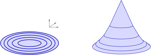
Figure 1: (a) The fuzzy plane. (b) The fuzzy BIon. This configuration can be obtained by pulling the fuzzy plane into the $z$ direction.

Our final confirmation is to check the preservation of 1/4 supersymmetry. In this case the killing spinor equation $\delta\Theta=0$ becomes

$$0 =\Big{(}D_{t}X^{i}\Gamma^{0i}+\frac{i}{2\lambda}[X^{i},X^{j}]\Gamma^{ij}\Big{)}P_{+}\epsilon+P_{+}\epsilon^{\prime}$$ (17)

$$=\pm\frac{i}{\lambda}\big{(}[X^{3},X^{1}]\Gamma^{01}+[X^{3},X^{2}]\Gamma^{02}\big{)}P_{+}\big{(}1\mp\Gamma^{03}\Gamma_{11}\big{)}\epsilon+\frac{i}{\lambda}[X^{1},X^{2}]P_{+}\Gamma^{12}\epsilon+P_{+}\epsilon^{\prime},$$

where $\epsilon$ and $\epsilon^{\prime}$ are constant Majorana spinors and $P_{+}=(1+\Gamma_{11})/2$. Thus we see that 1/4 supersymmetry is preserved when

$$\epsilon^{\prime}=\frac{b}{\lambda}\Gamma^{0}\epsilon,\qquad\epsilon=\frac{1\pm\Gamma^{03}\Gamma_{11}}{2}\frac{1+\Gamma^{012}}{2}\epsilon_{0},$$ (18)

where $\epsilon_{0}$ is an arbitrary constant Majorana spinor.

4 The Effective Action for the Fuzzy BIon

In the previous section we obtained the fuzzy BIon configuration as the classical solution of the BFSS matrix theory. We also checked that the fuzzy BIon preserves 1/4 supersymmetry of type IIA superstring theory. Now it is natural to ask whether the effective action for D0-branes which is described by the nonabelian Born-Infeld action contains the same solution. In this section we do not prove it directly, but construct the effective action for the fuzzy BIon by analyzing the nonabelian Born-Infeld action for D0-branes. We show that, with some conditions, the effective action obtained in this way correctly reproduce that for the BIon configuration in the continuous limit.

The nonabelian Born-Infeld action is given by refs. [11, 12, 13]. In the background of the flat space-time, when we set $X^{4}=\cdots=X^{9}=0$, this action is transformed into the form[7]

$$S_{\text{D}0} =-T_{0}\!\int\!dt\text{Tr}\sqrt{1-(D_{t}X^{i})^{2}-\frac{1}{2\lambda^{2}}[X^{i},X^{j}]^{2}+\frac{1}{4\lambda^{2}}\big{(}\epsilon_{ijk}\big{\{}D_{t}X^{i},[X^{j},X^{k}]\big{\}}\big{)}^{2}},$$ (19)

where $i,j,k=1,2,3$ and $\{A,B\}\equiv(AB+BA)/2$. Now we choose representations of three adjoint scalars $X^{1}$, $X^{2}$, $X^{3}$ and a gauge field $A_{t}$ as

$$X^{1}_{mn} =\frac{1}{2}\rho e^{i\theta}\big{|}_{m+1/2}\delta_{m+1,n}+\frac{1}{2}\rho e^{-i\theta}\big{|}_{m-1/2}\delta_{m,n+1},$$

$$X^{2}_{mn} =\frac{i}{2}\rho e^{i\theta}\big{|}_{m+1/2}\delta_{m+1,n}-\frac{i}{2}\rho e^{-i\theta}\big{|}_{m-1/2}\delta_{m,n+1},$$ (20)

$$X^{3}_{mn} =z|_{m}\delta_{m,n},\qquad A_{t\,mn}=a|_{m}\delta_{m,n}.$$

The notation $|_{m}$ is employed to show functions before this have the subscript $m$. Here the elements $\rho_{m+1/2}$, $\theta_{m+1/2}$, $z_{m}$ and $a_{m}$ are functions of the time $t$. Then by introducing the following definitions

$$\delta z|_{m+1/2}=z|_{m+1}-z|_{m},$$

$$\delta a|_{m+1/2}=a|_{m+1}-a|_{m},$$

$$\rho^{2}\delta z^{2}|_{m}=\frac{1}{2}\big{(}\rho^{2}\delta z^{2}|_{m+1/2}+\rho^{2}\delta z^{2}|_{m-1/2}\big{)},$$

$$\delta\rho^{2}|_{m}=\rho^{2}|_{m+1/2}-\rho^{2}|_{m-1/2},$$ (21)

$$\dot{\rho}^{2}|_{m}=\frac{1}{2}\big{(}\dot{\rho}^{2}|_{m+1/2}+\dot{\rho}^{2}|_{m-1/2}\big{)},$$

$$\rho^{2}(\dot{\theta}-\delta a)^{2}|_{m}=\frac{1}{2}\big{\{}\rho^{2}(\dot{\theta}-\delta a)^{2}|_{m+1/2}+\rho^{2}(\dot{\theta}-\delta a)^{2}|_{m-1/2}\big{\}},$$

$$\rho\dot{\rho}\delta z|_{m}=\frac{1}{2}\big{(}\rho\dot{\rho}\delta z|_{m+1/2}+\rho\dot{\rho}\delta z|_{m-1/2}\big{)},$$

after some calculations, the effective action (19) is evaluated as

$$S_{\text{D}0} =-T_{0}\!\int\!dt\sum_{m}\bigg{[}1+\Big{\{}-\dot{z}^{2}+\frac{1}{\lambda^{2}}\rho^{2}\delta z^{2}\Big{\}}$$

$$\qquad\qquad\qquad\qquad+\lambda^{2}\Big{\{}-\frac{1}{\lambda^{2}}\rho^{2}(\dot{\theta}-\delta a)^{2}+\frac{1}{4\lambda^{4}}(\delta\rho^{2})^{2}-\frac{1}{\lambda^{2}}\dot{\rho}^{2}\Big{\}}$$ (22)

$$\qquad\qquad\qquad\qquad-\lambda^{2}\Big{\{}\frac{1}{2\lambda^{2}}\dot{z}\delta\rho^{2}-\frac{1}{\lambda^{2}}\rho\dot{\rho}\delta z\Big{\}}^{2}\bigg{]}^{1/2}\bigg{|}_{m}.$$

Note that the interior of the square root is proportional to the identity matrix and the trace operation is simply replaced with the sum.

Let us return to the case of the fuzzy BIon configuration. Now we add a scalar fluctuation $\hat{z}|_{m}$ and gauge fluctuations $a_{\rho}|_{m+1/2}$, $a_{\phi}|_{m+1/2}$ and $a_{t}|_{m}$ around the fuzzy BIon configuration (12) and (14) like

$$X^{1}_{mn} =\frac{1}{2}\big{(}\rho^{c}+la_{\phi}\big{)}e^{ila_{\rho}}\big{|}_{m+1/2}\delta_{m+1,n}+\frac{1}{2}\big{(}\rho^{c}+la_{\phi}\big{)}e^{-ila_{\rho}}\big{|}_{m-1/2}\delta_{m,n+1},$$

$$X^{2}_{mn} =\frac{i}{2}\big{(}\rho^{c}+la_{\phi}\big{)}e^{ila_{\rho}}\big{|}_{m+1/2}\delta_{m+1,n}-\tfrac{i}{2}\big{(}\rho^{c}+la_{\phi}\big{)}e^{-ila_{\rho}}\big{|}_{m-1/2}\delta_{m,n+1},$$ (23)

$$X^{3}_{mn} =\big{(}z^{c}+\hat{z}\big{)}\big{|}_{m}\delta_{m,n},\qquad A_{t\,mn}=\big{(}a^{c}+a_{t}\big{)}\big{|}_{m}\delta_{m,n}.$$

Here we defined $l|_{m+1/2}=b/\rho^{c}|_{m+1/2}$ which is interpreted as a separation between $m$th and $(m+1)$th segments. We also define $\rho^{c}|_{m}=(\rho^{c}|_{m+1/2}+\rho^{c}|_{m-1/2})/2$ and $l|_{m}=b/\rho^{c}|_{m}$ for later use. Now the definitions (21) are translated into the forms

$$\delta z|_{m+1/2}=\frac{b}{\rho^{c}}\Big{(}\frac{L}{\rho^{c}}\!+\!\hat{z}^{\prime}\Big{)}\Big{|}_{m+1/2},\qquad\qquad\;\,\hat{z}^{\prime}|_{m+1/2}=\frac{\hat{z}|_{m+1}-\hat{z}|_{m}}{l|_{m+1/2}},$$

$$\delta a|_{m+1/2}=\frac{b}{\rho^{c}}\Big{(}\!\!\pm\!\frac{L}{\lambda\rho^{c}}\!+\!a^{\prime}_{t}\Big{)}\Big{|}_{m+1/2},\qquad\quad a^{\prime}_{t}|_{m+1/2}=\frac{a_{t}|_{m+1}-a_{t}|_{m}}{l|_{m+1/2}},$$

$$\delta\rho^{2}|_{m}\cong\frac{2b^{2}}{\rho^{c}}\Big{(}\frac{\rho^{c}}{b}\!+\!a^{\prime}_{\phi}\Big{)}\Big{|}_{m},\qquad\qquad\qquad\;\;a^{\prime}_{\phi}|_{m}=\frac{a_{\phi}|_{m+1/2}-a_{\phi}|_{m-1/2}}{l|_{m}},$$

$$\rho^{2}\delta z^{2}|_{m}\cong\frac{1}{2}\Big{\{}b^{2}\Big{(}\frac{L}{\rho^{c}}\!+\!\hat{z}^{\prime}\Big{)}^{2}\Big{|}_{m+1/2}\!\!+b^{2}\Big{(}\frac{L}{\rho^{c}}\!+\!\hat{z}^{\prime}\Big{)}^{2}\Big{|}_{m-1/2}\Big{\}}\equiv b^{2}\Big{(}\frac{L}{\rho^{c}}\!+\!\hat{z}^{\prime}\Big{)}^{2}\Big{|}_{m},$$ (24)

$$\dot{\rho}^{2}|_{m}=\frac{1}{2}\Big{(}\frac{b^{2}}{\rho^{c\,2}}\dot{a}_{\phi}^{2}\Big{|}_{m+1/2}\!\!+\frac{b^{2}}{\rho^{c\,2}}\dot{a}_{\phi}^{2}\Big{|}_{m-1/2}\Big{)}\equiv\frac{b^{2}}{\rho^{c\,2}}\dot{a}_{\phi}^{2}\Big{|}_{m},$$

$$\rho^{2}(\dot{\theta}\!-\!\delta a)^{2}|_{m}\cong\frac{1}{2}\Big{\{}b^{2}\Big{(}\!\!\mp\!\frac{L}{\lambda\rho^{c}}\!+\!f_{t\rho}\Big{)}^{2}\Big{|}_{m+1/2}\!\!+b^{2}\Big{(}\!\!\mp\!\frac{L}{\lambda\rho^{c}}\!+\!f_{t\rho}\Big{)}^{2}\Big{|}_{m-1/2}\Big{\}}\equiv b^{2}\Big{(}\!\!\mp\!\frac{L}{\lambda\rho^{c}}\!+\!f_{t\rho}\Big{)}^{2}\Big{|}_{m},$$

$$\rho\dot{\rho}\delta z|_{m}\cong\frac{1}{2}\Big{\{}\frac{b^{2}}{\rho^{c}}\Big{(}\frac{L}{\rho^{c}}\!+\!\hat{z}^{\prime}\Big{)}\dot{a}_{\phi}\Big{|}_{m+1/2}\!\!+\frac{b^{2}}{\rho^{c}}\Big{(}\frac{L}{\rho^{c}}\!+\!\hat{z}^{\prime}\Big{)}\dot{a}_{\phi}\Big{|}_{m-1/2}\Big{\}}\equiv\frac{b^{2}}{\rho^{c}}\Big{(}\frac{L}{\rho^{c}}\!+\!\hat{z}^{\prime}\Big{)}\dot{a}_{\phi}\Big{|}_{m}.$$

The symbol $\cong$ is used when we ignore higher order terms on $la_{\phi}/\rho^{c}|_{m}$. By substituting these values into (22), we obtain the effective action for the fuzzy BIon configuration,

$$S_{\text{D}0} \cong-T_{0}\!\int\!dt\sum_{m}\frac{l\rho^{c}}{b}\bigg{[}1+\Big{\{}-\dot{\hat{z}}^{2}+\frac{b^{2}}{\lambda^{2}}\Big{(}\frac{L}{\rho^{c}}+\hat{z}^{\prime}\Big{)}^{2}\Big{\}}$$

$$\qquad\qquad+\lambda^{2}\Big{\{}-\frac{b^{2}}{\lambda^{2}}\Big{(}\mp\frac{L}{\lambda\rho^{c}}+f_{t\rho}\Big{)}^{2}+\frac{b^{4}}{\lambda^{4}\rho^{c\,2}}\Big{(}\frac{\rho^{c}}{b}+a^{\prime}_{\phi}\Big{)}^{2}-\frac{b^{2}}{\lambda^{2}\rho^{c\,2}}\dot{a}_{\phi}^{2}\Big{\}}$$ (25)

$$\qquad\qquad-\lambda^{2}\Big{\{}\frac{b^{2}}{\lambda^{2}\rho^{c}}\dot{\hat{z}}\Big{(}\frac{\rho^{c}}{b}+a^{\prime}_{\phi}\Big{)}-\frac{b^{2}}{\lambda^{2}\rho^{c}}\Big{(}\frac{L}{\rho^{c}}+\hat{z}^{\prime}\Big{)}\dot{a}_{\phi}\Big{\}}^{2}\bigg{]}^{1/2}\bigg{|}_{m}.$$

Note that we used the relations $\rho^{c}l|_{m+1/2}=\rho^{c}l|_{m}=b$. Let us consider that $l_{m}$ are sufficiently small and take the continuous limit. Then the above effective action for the fuzzy BIon reaches to

$$S_{\text{D}0} =-\frac{T_{0}}{b}\!\int\!dtd\rho\rho\bigg{[}1+\Big{\{}-\dot{\hat{z}}^{2}+\frac{b^{2}}{\lambda^{2}}\Big{(}\frac{L}{\rho}+\hat{z}^{\prime}\Big{)}^{2}\Big{\}}$$

$$\qquad\qquad+\lambda^{2}\Big{\{}-\frac{b^{2}}{\lambda^{2}}\Big{(}\mp\frac{L}{\lambda\rho}+f_{t\rho}\Big{)}^{2}+\frac{b^{4}}{\lambda^{4}\rho^{2}}\Big{(}\frac{\rho}{b}+a^{\prime}_{\phi}\Big{)}^{2}-\frac{b^{2}}{\lambda^{2}\rho^{2}}\dot{a}_{\phi}^{2}\Big{\}}$$ (26)

$$\qquad\qquad-\lambda^{2}\Big{\{}\frac{b^{2}}{\lambda^{2}\rho}\dot{\hat{z}}\Big{(}\frac{\rho}{b}+a^{\prime}_{\phi}\Big{)}-\frac{b^{2}}{\lambda^{2}\rho}\Big{(}\frac{L}{\rho}+\hat{z}^{\prime}\Big{)}\dot{a}_{\phi}\Big{\}}^{2}\bigg{]}^{1/2}.$$

In order to justify this action, we should compare with the effective action for the BIon configuration.

The effective action for the D2-brane is described by

$$S_{\text{D2}}=-T_{2}\int dtd\rho d\phi\rho\sqrt{1+\partial_{\alpha}z\partial^{\alpha}z+\frac{\lambda^{2}}{2}F_{\alpha\beta}F^{\alpha\beta}-\frac{\lambda^{2}}{4}(\epsilon^{\alpha\beta\gamma}\partial_{\alpha}zF_{\beta\gamma})^{2}},$$ (27)

where indices are raised or lowered by the metric $ds^{2}=-dt^{2}+d\rho^{2}+\rho^{2}d\phi^{2}$ and $\epsilon^{t\rho\phi}=1/\rho$. The fluctuations around the BIon solution is given by

$$z=z_{0}+L\ln\rho+\hat{z}(t,\rho),$$

$$F_{t\rho}=\pm\frac{L}{\lambda\rho}+f_{t\rho}(t,\rho),$$ (28)

$$F_{\rho\phi}=\frac{\rho}{b}+a^{\prime}_{\phi}(t,\rho),$$

$$F_{t\phi}=\dot{a}_{\phi}(t,\rho).$$

We assumed that fluctuations $\hat{z}$, $a_{t}$, $a_{\rho}$ and $a_{\phi}$ do not depend on the angular direction $\phi$. By substituting these into the effective action, we obtain

$$S_{\text{D2}} =-2\pi T_{2}\int dtd\rho\rho\bigg{[}1+\Big{\{}-\dot{\hat{z}}^{2}+\Big{(}\frac{L}{\rho}+\hat{z}^{\prime}\Big{)}^{2}\Big{\}}$$

$$\qquad\qquad\qquad\qquad\;+\lambda^{2}\Big{\{}-\Big{(}\mp\frac{L}{\lambda\rho}+f_{t\rho}\Big{)}^{2}+\frac{1}{\rho^{2}}\Big{(}\frac{\rho}{b}+a^{\prime}_{\phi}\Big{)}^{2}-\frac{1}{\rho^{2}}{\dot{a}_{\phi}}^{2}\Big{\}}$$ (29)

$$\qquad\qquad\qquad\qquad\;-\lambda^{2}\Big{\{}\frac{1}{\rho}\dot{\hat{z}}\Big{(}\frac{\rho}{b}+a^{\prime}_{\phi}\Big{)}-\frac{1}{\rho}\Big{(}\frac{L}{\rho}+\hat{z}^{\prime}\Big{)}\dot{a}_{\phi}\Big{\}}^{2}\bigg{]}^{1/2}.$$

From these we see that the action (26) coincides with the action (29) in the case of $b=\lambda$. This result is the same as that in ref. [7]. The condition $b=\lambda$ suggests that a D0-brane can transform into a D2-brane with the area $2\pi\lambda$.

5 Conclusion

In this paper we construct the fuzzy BIon configuration in the framework of BFSS matrix theory. This solution equips the properties of the BIon solution which represents a fundamental string ending on a bound state of a D2-brane and D0-branes. For instance, the differential equation (7) for the BIon corresponds to the discrete equations (15) for the fuzzy BIon. We also checked that the fuzzy BIon preserves 1/4 supersymmetry of type IIA superstring theory.

In section 4, we construct the effective action for the fuzzy BIon configuration by analyzing the nonabelian Born-Infeld action for D0-branes. In the continuous limit, this action coincides with the effective action for the BIon configuration, in the case of $b=\lambda$. This means that a D0-brane can transform into a D2-brane with the area $2\pi\lambda$. This fact is also supported by the energy conservation that $T_{0}=2\pi\lambda T_{2}$. With these nontrivial confirmations, we conclude that the fuzzy BIon configuration is also a solution of nonabelian Born-Infeld action for D0-branes.

It is important to note that only a fundamental string exists around the origin of the fuzzy BIon. This would make us possible to compute the interaction between a fundamental string and D0-branes in the framework of BFSS matrix theory. It is also interesting to generalize the fuzzy BIon configuration in the curved space background[14].

References

-
[1]
D. Mateos and P. K. Townsend,
“Supertubes”,
Phys. Rev. Let. 87 (2001) 011602; hep-th/0103030. - [2] R. G. Leigh, Mod. Phys. Lett. A4 (1989) 2767.
- [3] M. Aganagic, C. Popescu and J. H. Schwarz, “D-brane Actions with Local Kappa Symmetry” Phys. Lett. B393 (1997) 311-315, hep-th/9610249.
-
[4]
E. Bergshoeff and P. K. Townsend,
“Super D-branes”,
Nucl. Phys. B490 (1997) 145-162, hep-th/9611173. - [5] T. Banks, W. Fischler, S.H. Shenker and L. Susskind, “M Theory as a Matrix Model: A Conjecture”, Phys. Rev. D55 (1997) 5112-5128; hep-th/9610043.
-
[6]
Y. Hyakutake,
“Torus-like Dielectric D2-brane”,
JHEP 0105 (2001) 013; hep-th/0103146. - [7] Y. Hyakutake “Notes on the Construction of the D2-brane from Multiple D0-branes”, hep-th/0302190.
-
[8]
T. Banks, N. Seiberg, S. H. Shenker,
“Branes from Matrices”,
Nucl. Phys. B490 (1997) 91-106; hep-th/9612157. -
[9]
D. Bak, Ki-Myeong Lee,
“Noncommutative Supersymmetric Tubes”,
Phys. Lett. B509 (2001) 168-174; hep-th/0103148. - [10] Y. Hyakutake, “Expanded Strings in the Background of NS5-branes via a M2-brane, a D2-brane and D0-branes”, JHEP 0201 (2002) 021; hep-th/0112073.
-
[11]
A. A. Tseytlin,
“Born-Infeld action, supersymmetry and string theory”,
hep-th/9908105. - [12] A. A. Tseytlin, “On Nonabelian Generalization of Born-Infeld Action in String Theory”, Nucl. Phys. B501 (1997) 41-52; hep-th/9701125.
- [13] R. C. Myers, “Dielectric Branes”, JHEP 9912 (1999) 022; hep-th/9910053.
- [14] D. K. Park, S. Tamaryan, H. J. W. Muller-Kirsten, “General Criterion for the Existence of Supertube and BIon in Curved Target Space”, hep-th/0302145.
-
[15]
Nakwoo Kim,
“More on Membranes in Matrix Theory”,
Phys. Rev. D59 (1999) 067901, hep-th/9808166.