More on ghost condensation in Yang-Mills theory: BCS versus Overhauser effect and the breakdown of the Nakanishi-Ojima annex $SL(2,R)$ symmetry

Abstract

We analyze the ghost condensates $\left\langle f^{abc}c^{b}c^{c}\right\rangle$, $\left\langle f^{abc}\overline{c}^{b}\overline{c}^{c}\right\rangle$ and $\left\langle f^{abc}\overline{c}^{b}c^{c}\right\rangle$ in Yang-Mills theory in the Curci-Ferrari gauge. By combining the local composite operator formalism with the algebraic renormalization technique, we are able to give a simultaneous discussion of $\left\langle f^{abc}c^{b}c^{c}\right\rangle$,$\left\langle f^{abc}\overline{c}^{b}\overline{c}^{c}\right\rangle$ and $\left\langle f^{abc}\overline{c}^{b}c^{c}\right\rangle$, which can be seen as playing the role of the BCS, respectively Overhauser effect in ordinary superconductivity. The Curci-Ferrari gauge exhibits a global continuous symmetry generated by the Nakanishi-Ojima ($NO$) algebra. This algebra includes, next to the (anti-)BRST transformation, a $SL(2,R)$ subalgebra. We discuss the dynamical symmetry breaking of the $NO$ algebra through these ghost condensates. Particular attention is paid to the Landau gauge, a special case of the Curci-Ferrari gauge.

LTH–579

1 Introduction

Vacuum condensates play an important role in quantum field theory. They can be used to parametrize some non-perturbative effects. If one wants to attach a physical meaning to a certain condensate in case of a gauge theory, it should evidently be gauge invariant. Two well known examples in the context of QCD are the gluon condensate $\left\langle F_{\mu\nu}^{2}\right\rangle$ and the quark condensate $\left\langle\overline{q}q\right\rangle$.

Recently, there was a growing interest for a mass dimension 2 condensate in (quarkless) QCD in the Landau gauge, see e.g. [1, 2, 3, 4, 5, 6]. Unfortunately, no local gauge invariant operator with mass dimension 2 exists. However, a non-local gauge invariant dimension 2 operator can be constructed by minimizing $A^{2}$ along each gauge orbit, namely $A^{2}_{\tiny{\textrm{min}}}\equiv(VT)^{-1}\min_{U}\int d^{4}x\left(A_{\mu}^{U}\right)^{2}$ with $VT$ the space time volume and $U$ a generic $SU(N)$ transformation. This operator is related to the Gribov region as well as the so-called fundamental modular region (FMR), which is the set of absolute minima of $\int d^{4}x\left(A_{\mu}^{U}\right)^{2}$ [7, 8, 9]. In particular, in the Landau gauge $\partial_{\mu}A^{\mu}=0$, it turned out that $A^{2}_{\tiny{\textrm{min}}}$ reduces to the local operator $A^{2}$. This gives a meaning to the condensate $\left\langle A^{2}\right\rangle$. In [6], an effective action was constructed in the weak coupling for the $\left\langle A^{2}\right\rangle$ condensate by means of the local composite operator technique (LCO) and it was shown that $\left\langle A^{2}\right\rangle\neq 0$ is dynamically favoured since it lowers the vacuum energy. Due to this condensate, the gluons achieved a mass.

In this article, we will discuss other condensates of mass dimension 2 [10], namely pure ghost condensates of the type $\left\langle f^{abc}c^{b}c^{c}\right\rangle$, $\left\langle f^{abc}\overline{c}^{b}\overline{c}^{c}\right\rangle$ and $\left\langle f^{abc}\overline{c}^{b}c^{c}\right\rangle$. Historically, these condensates came to attention in [11, 12, 13, 14] in the context of $SU(2)$ Yang-Mills theory in the Maximal Abelian gauge. This is a partial non-linear gauge fixing which requires the introduction of a four ghost interaction term for consistency. A decomposition, by means of a Hubbard-Stratonovich auxiliary field, similar to the one of the 4-fermion interaction of the Gross-Neveu model [15], allowed to construct a 1-loop effective potential, leading to a non-trivial minimum for the ghost condensate corresponding to $\left\langle f^{abc}\overline{c}^{b}c^{c}\right\rangle$. It was recognized in [11, 12, 13] that this condensate signals the breakdown of a global $SL(2,R)$ symmetry of the $SU(2)$ Maximal Abelian gauge model. The ghost condensate was used to find a mass for the off-diagonal gluons, and thereby a certain evidence for the Abelian dominance was established [14]. It has been shown since then that the ghost condensate gives in fact a tachyonic mass [16].

It is worth mentioning that a simple decomposition of the 4-fermion interaction might cause troubles with the renormalizability beyond the 1-loop order. For instance, in the case of the Gross-Neveu model, this procedure requires the introduction of ad hoc counterterms to maintain finiteness [17, 18]. A similar problem can be expected with the 4-ghost interaction. The LCO procedure gave an outcome to this problem [17].

Another issue that deserves clarification is the fact that with a different decomposition, different ghost condensates appear [19], corresponding to the Faddeev-Popov charged condensates $\left\langle f^{abc}c^{b}c^{c}\right\rangle$ and $\left\langle f^{abc}\overline{c}^{b}\overline{c}^{c}\right\rangle$. The existence of several channels for the ghost condensation has a nice analogy in the theory of superconductivity, known as the BCS versus Overhauser effect. The BCS channel corresponds to the charged particle-particle and hole-hole pairing [20, 21], while the Overhauser channel to the particle-hole pairing [22, 23]. In the present case, the Faddeev-Popov charged condensates $\left\langle f^{abc}\overline{c}^{b}\overline{c}^{c}\right\rangle$ and $\left\langle f^{abc}c^{b}c^{c}\right\rangle$ would correspond to the BCS channel, while $\left\langle f^{abc}\overline{c}^{b}c^{c}\right\rangle$ to the Overhauser channel. The question is whether one of these effects would be favoured. A simultaneous discussion of both effects is necessary to find out if one vacuum is more stable than the other.

It is appealing that by now the ghost condensates have been observed also in a class of non-linear generalized covariant gauges [24, 25], the so-called Curci-Ferrari gauges, again by the decomposition of a 4-ghost interaction [28]. The Curci-Ferrari gauge has the Landau gauge as a special case. Although the Landau gauge lacks a 4-ghost interaction, it has been shown that the ghost condensation also takes place in this gauge [29]. Evidently, this was not possible by the decomposition of a 4-point interaction. However, the combination of the LCO method [6, 30] with the algebraic renormalization formalism [31, 32] allowed for a clean treatment of the ghost condensation in the Landau gauge.

It seems thus that the ghost condensation takes place in a variety of gauges: the Landau gauge, the Curci-Ferrari gauge and the Maximal Abelian gauge. It is known that the Landau gauge and Curci-Ferrari gauge exhibit a global continuous symmetry, generated by the so-called Nakanishi-Ojima algebra [33, 34, 35, 36, 37, 38]. This algebra contains, next to the BRST and anti-BRST transformations, a $SL(2,R)$ subalgebra generated by the Faddeev-Popov ghost number and 2 other operators, $\delta$ and $\overline{\delta}$. Moreover, $\delta$ and $\overline{\delta}$ mutually transform the ghost operators $f^{abc}c^{b}c^{c}$, $f^{abc}\overline{c}^{b}\overline{c}^{c}$ and $f^{abc}\overline{c}^{b}c^{c}$ into each other. It is then apparent that the ghost condensation can appear in several channels like the BCS and Overhauser channel, and that a non-vanishing vacuum expectation value for the ghost operators indicates a breakdown of this $SL(2,R)$ symmetry.

Recently, it has been shown that the same $NO$ invariance of the Landau and Curci-Ferrari gauge can be maintained in the Maximal Abelian gauge for any value of $N$ [39]. Apparently, an intimate connection exists between the $NO$ symmetry and the appearance of the ghost condensates, since all gauges where the ghost condensates has been proven to occur, have the global $NO$ invariance.

The aim of this article is to provide an answer to the aforementioned issues. We will discuss the Curci-Ferrari gauge. For explicit calculations, we will restrict ourselves to the Landau gauge for $SU(2)$. The presented general arguments are however neither depending on the choice of the gauge parameter, nor on the value of $N$. The paper is organized as follows. In section 2, we show that it is possible to introduce a set of external sources for the ghost operators, according to the LCO method, and this without spoiling the $NO$ invariance. Employing the algebraic renormalization technique [31, 32], it can then be checked that the proposed action can be renormalized. In section 3, the effective potential for the ghost condensates is evaluated. By contruction, this effective potential, incorporating the BCS as well as the Overhauser channel, is finite up to any order and obeys a homogeneous renormalization group equation. Next, in section 4, we pay attention to the dynamical symmetry breaking of the $NO$ algebra due to the ghost condensates. Because of the $SL(2,R)$ invariance of the presented framework, it becomes clear that a whole class of equivalent, non-trivial vacua exist. The Overhauser and the BCS vacuum are important special cases. Notice that a nonvanishing condensate $\left\langle f^{abc}c^{b}c^{c}\right\rangle\neq 0$ could seem to pose a problem for the Faddeev-Popov ghost number symmetry and for the BRST symmetry, two basic properties of a quantized gauge theory. However, we shall be able to show that one can define a nilpotent BRST and a Faddeev-Popov symmetry in any possible ghost condensed vacuum. The existence of the $NO$ symmetry plays a key role in this. Since the ghost condensates carry a color index, we also spend some words on the global $SU(N)$ color symmetry. Here, we can provide an argument that, thanks to the existence of the condensate $\left\langle A^{2}\right\rangle$ and of its generalization $\left\langle\frac{1}{2}A^{2}+\alpha\overline{c}c\right\rangle$ in the Curci-Ferrari gauge [40], the breaking of the color symmetry, induced by the ghost condensates, should be located in the unphysical part of the Hilbert space. Furthermore, we argue why no physical Goldstone particles should appear by means of the quartet mechanism [41]. Section 5 handles the generalization of the results to the case with quarks included. In section 6, we give an outline of future research where the gluon and ghost condensates can play a role. We end with conclusions in section 7. Technical details are collected in the Appendices A and B.

2 The set of external sources for both BCS and Overhauser channel

2.1 Introduction of the LCO sources

For a thorough introduction to the local composite operator (LCO) formalism and to the algebraic renormalization technique, the reader is referred to [6, 30], respectively [31].

According to the LCO method, the first step in the analysis of the ghost condensation in both channels is the introduction of a suitable system of external sources. Generalizing the construction done in the pure BCS case [29], it turns out that the simultaneous presence of both channels is achieved by considering the following BRST invariant external action

$$S_{LCO} = s\int d^{4}x\left(L^{a}c^{a}+\lambda^{a}\left(b^{a}-gf^{abc}\overline{c}^{b}c^{c}\right)+\zeta\eta^{a}L^{a}-\frac{1}{2}\eta^{a}gf^{abc}\overline{c}^{b}\overline{c}^{c}+\frac{1}{2}\rho\lambda^{a}\omega^{a}-\omega^{a}\overline{c}^{a}\;\right)$$

$$= \int d^{4}x\left(\frac{1}{2}L^{a}gf^{abc}c^{b}c^{c}-\frac{1}{2}\tau^{a}gf^{abc}\overline{c}^{b}\overline{c}^{c}+\eta^{a}gf^{abc}b^{b}\overline{c}^{c}+\zeta\tau^{a}L^{a}\right.$$

$$- \left.\omega^{a}gf^{abc}\overline{c}^{b}c^{c}+\;\lambda^{a}gf^{abc}b^{b}c^{c}-\frac{1}{2}\lambda^{a}g^{2}f^{abc}\overline{c}^{b}f^{cmn}c^{m}c^{n}+\frac{1}{2}\rho\omega^{a}\omega^{a}\right)$$

The BRST transformation $s$ is defined for the fields $A_{\mu}^{a}$, $c^{a}$, $\overline{c}^{a}$, $b^{a}$ as

$$sA_{\mu}^{a} = -D_{\mu}^{ab}c^{b}$$

$$sc^{a} = \frac{g}{2}f^{abc}c^{b}c^{c}$$

$$s\overline{c}^{a} = b^{a}$$

$$sb^{a} = 0$$ (2.2)

with

$$D_{\mu}^{ab}=\partial_{\mu}\delta^{ab}+gf^{acb}A_{\mu}^{c}$$ (2.3)

the adjoint covariant derivative.

The external sources $L^{a}$, $\tau^{a}$, $\lambda^{a}$, $\omega^{a}$, $\eta^{a}$ transform as

$$s\eta^{a} = \tau^{a}\;,\;\;\;\;s\tau^{a}=\;0\;,$$ (2.4)

$$s\lambda^{a} = \omega^{a}\;,\;\;\;s\omega^{a}=\;0\;,$$

$$sL^{a} = 0$$

$$L^{a}$$

(2.5)

¿From expression (LABEL:slco) one sees that the sources $L^{a}$, $\tau^{a}$ couple to the ghost operators $gf^{abc}c^{b}c^{c}$, $gf^{abc}\overline{c}^{b}\overline{c}^{c}$ of the BCS channel, while $\omega^{a}$ accounts for the Overhauser channel $gf^{abc}\overline{c}^{b}c^{c}$. As far as the BRST invariance is the only invariance required for the external action (LABEL:slco), the LCO parameters $\zeta$ and $\rho$ are independent. However, it is known that both the Landau and the Curci-Ferrari gauge display a larger set of symmetries, giving rise to the $NO$ algebra [24, 25, 33, 34, 35, 36, 37, 38, 39]. It is worth remarking that the whole $NO$ algebra can be extended also in the presence of the external action $S_{LCO}$, provided that the two parameters $\zeta$ and $\rho$ obey the relationship

$$\rho=2\zeta$$ (2.6)

In other words, the requirement of invariance of $S_{LCO}$ under the whole $NO$ algebra allows for a unique parameter in expression (LABEL:slco). In order to introduce the generators of the $NO$ algebra, let us begin with the anti-BRST transformation $\overline{s}$

$$\overline{s}A_{\mu}^{a} = -D_{\mu}^{ab}\overline{c}^{b}$$

$$\overline{s}c^{a} = -b^{a}+gf^{abc}c^{b}\overline{c}^{c}$$

$$\overline{s}\overline{c}^{a} = \frac{g}{2}f^{abc}\overline{c}^{b}\overline{c}^{c}$$

$$\overline{s}b^{a} = -gf^{abc}b^{b}\overline{c}^{c}$$ (2.7)

Extending $\overline{s}$ to the external LCO sources as

$$\overline{s}\eta^{a} = -\omega^{a}\;,\;\;\;\;\overline{s}\tau^{a}=\;0$$ (2.8)

$$\overline{s}\lambda^{a} = L^{a}\;,\;\;\;\;\;\;\overline{s}\omega^{a}=\;0$$

$$\overline{s}L^{a} = 0$$

one easily verifies that

$$\{s,\overline{s}\}=s\overline{s}+\overline{s}s=0$$ (2.9)

Furthermore, the requirement of invariance of $S_{LCO}$ under $\overline{s}$ fixes the parameter $\rho=2\zeta$, namely

$$\overline{s}S_{LCO}=0\;\Rightarrow\;\rho=2\zeta$$ (2.10)

This is best seen by observing that, when $\rho=2\zeta$, the whole action $S_{LCO}$ can be written as

$$S_{LCO}=s\overline{s}\int d^{4}x\left(\lambda^{a}c^{a}+\zeta\lambda^{a}\eta^{a}+\eta^{a}\overline{c}^{a}\right)$$ (2.11)

Concerning now the other generators $\delta$ and $\overline{\delta}$ of the $NO$ algebra, they can be introduced as follows

$$\delta\overline{c}^{a} = c^{a}$$

$$\delta b^{a} = \frac{g}{2}f^{abc}c^{b}c^{c}$$

$$\delta A_{\mu}^{a} = \delta c^{a}=0$$

$$\delta L^{a} = 2\omega^{a}$$

$$\delta\omega^{a} = -\tau^{a}$$

$$\delta\lambda^{a} = -\eta^{a}$$

$$\delta\tau^{a} = \delta\eta^{a}=0$$ (2.12)

and

$$\overline{\delta}c^{a} = \overline{c}^{a}$$

$$\overline{\delta}b^{a} = \frac{g}{2}f^{abc}\overline{c}^{b}\overline{c}^{c}$$

$$\overline{\delta}A_{\mu}^{a} = \overline{\delta}\overline{c}^{a}=0$$

$$\overline{\delta}\omega^{a} = L^{a}$$

$$\overline{\delta}\tau^{a} = -2\omega^{a}$$

$$\overline{\delta}\eta^{a} = -\lambda^{a}$$

$$\overline{\delta}L^{a} = \overline{\delta}\lambda^{a}=0$$ (2.13)

It holds that

$$\delta S_{LCO}=\overline{\delta}S_{LCO}=0$$ (2.14)

The operators $s$, $\overline{s}$, $\delta$, $\overline{\delta}$ and the Faddeev-Popov ghost number operator $\delta_{FP}$ give rise to the $NO$ algebra

$$s^{2} = 0\,,\,\,\,\,\,\,\,\,\,\,\,\overline{s}^{2}=0$$

$$\,\{s,\overline{s}\} = 0\,,\,\,\,\,\,\,\,\,\,\,[\delta,\overline{\delta}]=\delta_{\mathrm{FP}}\,,$$

$$[\delta,\delta_{\mathrm{FP}}] = -2\delta,\,\,\,[\overline{\delta},\delta_{\mathrm{FP}}]=2\overline{\delta}$$

$$[s,\delta_{\mathrm{FP}}] = -s\,,\,\,\,\,\,\,[\overline{s},\delta_{\mathrm{FP}}]=\overline{s}\,,$$

$$[s,\delta] = 0\,\,,\,\,\,\,\,\,\,\,[\overline{s},\overline{\delta}]=0\,,$$

$$[s,\overline{\delta}] = -\overline{s}\,\,,\,\,\,\,\,[\overline{s},\delta]=-s$$ (2.15)

In particular, $\delta_{FP}$, $\delta$, $\overline{\delta}$ generate a $SL(2,R)$ subalgebra. We remark that the $NO$ algebra can be established as an exact invariance of $S_{LCO}$ only when both channels are present. It is easy to verify indeed that setting to zero the external sources corresponding to one channel will imply the loss of the $NO$ algebra. This implies that a complete discussion of the ghost condensates needs sources for the BCS as well as for the Overhauser channel.

Let us also give, for further use, the expressions of the gauge fixed action in the presence of the LCO external sources for the Curci-Ferrari gauge.

$$S = S_{YM}+S_{GF+FP}+S_{LCO}$$

$$= -\frac{1}{4}\int d^{4}xF_{\mu\nu}^{a}F^{a\mu\nu}+s\overline{s}\int d^{4}x\left(\frac{1}{2}A_{\mu}^{a}A^{a\mu}+\lambda^{a}c^{a}+\zeta\lambda^{a}\eta^{a}+\eta^{a}\overline{c}^{a}-\frac{\alpha}{2}c^{a}\overline{c}^{a}\right)$$

with

$$S_{GF+FP} = \int d^{4}x\left(b^{a}\partial_{\mu}A^{a\mu}+\frac{\alpha}{2}b^{a}b^{a}+\overline{c}^{a}\partial^{\mu}D_{\mu}^{ab}c^{b}-\frac{\alpha}{2}gf^{abc}b^{a}\overline{c}^{b}c^{c}-\frac{\alpha}{8}g^{2}f^{abc}f^{cde}\overline{c}^{a}\overline{c}^{b}c^{d}c^{e}\right)$$

The renormalizability of the action (LABEL:scf) is discussed in the Appendix A.

The Curci-Ferrari gauge has the Landau gauge, $\alpha=0$, as interesting special case, see for example [40]. One sees that the difference between the two actions is due to the term $\alpha c^{a}\overline{c}^{a}$, which gives rise to a quartic ghost self interaction absent in the Landau gauge. The whole set of $NO$ invariances can be translated into functional identities which ensures the renormalizability of the model. In particular, concerning the counterterm contributions $\delta_{L}L^{a}gf^{abc}c^{b}c^{c}$, $\delta_{\tau}\tau^{a}gf^{abc}\overline{c}^{b}\overline{c}^{c}$ and $\delta_{\omega}\omega^{a}gf^{abc}\overline{c}^{b}c^{c}\;$, it is shown in the Appendix A that

$$\delta_{L}=\delta_{\tau}=\delta_{\omega}\equiv\delta_{2}$$ (2.18)

Consequently, the operators $gf^{abc}c^{b}c^{c}$, $gf^{abc}\overline{c}^{b}\overline{c}^{c}$ and $gf^{abc}\overline{c}^{b}c^{c}$ turn out to have the same anomalous dimension for any $\alpha$. As expected, this result is a consequence of the presence of the $NO$ symmetry. Moreover, in the Landau gauge, $\delta_{2}\equiv 0$ due to the nonrenormalization properties of the Landau gauge [31]. In [42], one can find an explicit proof that $\delta_{2}=0$.

2.2 A note on the choice of the hermiticity properties of the Faddeev-Popov ghosts

With our choice of ghosts $c$, respectively anti-ghosts $\overline{c}$, the hermiticity assignment

$$c^{{\dagger}} = c$$

$$\overline{c}^{{\dagger}} = -\overline{c}$$ (2.19)

is obeyed. This implies that $c$ and $\overline{c}$ are independent degrees of freedom and by a redefinition $i\overline{c}=\overline{c}^{\prime}$, we have real (anti-)ghost fields $c$ and $\overline{c}^{\prime}$. Another assignment that is used sometimes, reads

$$c^{{\dagger}} = \overline{c}$$ (2.20)

As it was explored in e.g. [38, 41], the former assignment is the correct one for a generic gauge. However, based on the additional ghost-anti-ghost symmetry in the Landau gauge, both formulations are equivalent. Moreover, this equivalence, which is related to the existence of the $SL(2,R)$ symmetry, can be maintained if the Landau gauge is generalized to the Curci-Ferrari gauge [43]. Since we are discussing the existence of $\left\langle f^{abc}\overline{c}^{b}c^{c}\right\rangle$, $\left\langle f^{abc}c^{b}c^{c}\right\rangle$ and $\left\langle f^{abc}\overline{c}^{b}\overline{c}^{c}\right\rangle$, which break the $SL(2,R)$ symmetry, the equivalence between the real formulation (2.2) and the complex one (2.20) might be altered. For example, if $\left\langle f^{abc}c^{b}c^{c}\right\rangle\neq\left\langle f^{abc}\overline{c}^{b}\overline{c}^{c}\right\rangle$, the ghost-anti-ghost symmetry is lost, as well as the usual ghost number symmetry. Throughout this article, we will use the prescription (2.2). We will return to the issue of the ghost number symmetry later in this article.

3 Effective potential for the ghost condensates

3.1 General considerations

Let us proceed with the construction of the effective potential for the ghost condensates in the Curci-Ferrari gauge. To decide which channel is favoured, we have to consider the 2 channels at once. We shall also treat the two LCO parameters $\rho$ and $\zeta$ for the moment as being independent and verify the relationship (LABEL:slco). Setting to zero the external sources $\eta$ and $\lambda$, we start from the action

$$S = S_{YM}+S_{GF+FP}+\int d^{4}x\left[-\omega^{a}gf^{abc}\overline{c}^{b}c^{c}+\frac{1}{2}\rho\omega^{a}\omega^{a}\right.$$ (3.1)

$$+ \left.\frac{1}{2}L^{a}gf^{abc}c^{b}c^{c}-\frac{1}{2}\tau^{a}gf^{abc}\overline{c}^{b}\overline{c}^{c}+\zeta\tau^{a}L^{a}\right]$$

Following [6, 30], the divergences proportional to $L\tau$ are cancelled by the counterterm $\delta\zeta\tau L$, and the divergences proportional to $\omega^{2}$ are cancelled by the counterterm $\frac{\delta\rho}{2}\omega^{2}$. Considering the bare Lagrangian associated to (3.1), we have

$$c_{b} = \sqrt{Z_{c}}c\hskip 28.45274pt\overline{c}_{b}=\sqrt{Z_{c}}\overline{c}$$ (3.2)

$$A_{b} = \sqrt{Z_{A}}A$$ (3.3)

$$g_{b} = \mu^{\varepsilon/2}Z_{g}g$$ (3.4)

$$L_{b} = \mu^{-\varepsilon/2}\frac{Z_{2}}{Z_{g}Z_{c}}L\hskip 28.45274pt\tau_{b}=\mu^{-\varepsilon/2}\frac{Z_{2}}{Z_{g}Z_{c}}\tau\hskip 28.45274pt\omega_{b}=\mu^{-\varepsilon/2}\frac{Z_{2}}{Z_{g}Z_{c}}\omega$$ (3.5)

where $Z_{2}=1+\delta_{2}$ (see (2.18)).
Furthermore,

$$\zeta_{b}\tau_{b}^{a}L_{b}^{a} = \mu^{-\varepsilon}\left(\zeta+\delta\zeta\right)\tau^{a}L^{a}$$ (3.6)

$$\frac{1}{2}\rho_{b}\omega_{b}^{a}\omega_{b}^{a} = \frac{1}{2}\mu^{-\varepsilon}\left(\rho+\delta\rho\right)\omega^{a}\omega^{a}$$ (3.7)

where it is understood that we are working with dimensional regularization in $d=4-\varepsilon$ dimensions. The above equations allow to derive the renormalization group equation of $\zeta$ and $\rho$

$$\mu\frac{d\zeta}{d\mu} = 2\gamma(g^{2})\zeta+\delta_{\zeta}(g^{2})$$ (3.8)

$$\mu\frac{d\rho}{d\mu} = 2\gamma(g^{2})\rho+\delta_{\rho}(g^{2})$$ (3.9)

where $\gamma(g^{2})$ denotes the anomalous dimension of the ghost operators $gf^{abc}\overline{c}^{b}c^{c}$, $gf^{abc}c^{b}c^{c}$ and $gf^{abc}\overline{c}^{b}\overline{c}^{c}$, given by

$$\gamma(g^{2})=\mu\frac{d}{d\mu}\ln\frac{Z_{2}}{Z_{g}Z_{c}}$$ (3.10)

$\delta_{\zeta}$ and $\delta_{\rho}$ are defined as

$$\delta_{\zeta}(g^{2}) = \left(\varepsilon-2\widehat{\gamma}(g^{2})-\beta(g^{2})\frac{\partial}{\partial g^{2}}-\alpha\gamma_{\alpha}(g^{2})\frac{\partial}{\partial\alpha}\right)\delta\zeta$$ (3.11)

$$\delta_{\rho}(g^{2}) = \left(\varepsilon-2\widehat{\gamma}(g^{2})-\beta(g^{2})\frac{\partial}{\partial g^{2}}-\alpha\gamma_{\alpha}(g^{2})\frac{\partial}{\partial\alpha}\right)\delta\rho$$ (3.12)

where $\beta(g^{2})=\mu\frac{dg^{2}}{d\mu}$ is the usual running of the coupling constant, in $d$ dimensions given by

$$\beta(g^{2})=-\varepsilon g^{2}-\frac{22}{3}g^{2}\frac{g^{2}N}{16\pi^{2}}-\frac{68}{3}g^{2}\left(\frac{g^{2}N}{16\pi^{2}}\right)^{2}+\cdots$$ (3.13)

while $\gamma_{\alpha}(g^{2})=\frac{\mu}{\alpha}\frac{d\alpha}{d\mu}$ denotes the running of the gauge parameter $\alpha$. We do not write the possible $\alpha$ dependence of the appearing renormalization group functions; for the explicit calculations in section 3.2, we will restrict ourselves to the Landau gauge. Therefore, we also do not write down the explicit value of $\gamma_{\alpha}(g^{2})$ since $\alpha\gamma_{\alpha}(g^{2})\equiv 0$ for $\alpha=0$.

$\widehat{\gamma}(g^{2})$ denotes the anomalous dimension of the sources $\omega$, $\tau$ and $L$. $\gamma(g^{2})$ and $\widehat{\gamma}(g^{2})$ are related by

$$\widehat{\gamma}(g^{2})=\frac{\varepsilon}{2}-\gamma(g^{2})$$ (3.14)

and therefore, the equations (3.11)-(3.12) can be rewritten as

$$\delta_{\zeta}(g^{2}) = \left(2\gamma(g^{2})-\beta(g^{2})\frac{\partial}{\partial g^{2}}-\alpha\gamma_{\alpha}(g^{2})\frac{\partial}{\partial\alpha}\right)\delta\zeta$$ (3.15)

$$\delta_{\rho}(g^{2}) = \left(2\gamma(g^{2})-\beta(g^{2})\frac{\partial}{\partial g^{2}}-\alpha\gamma_{\alpha}(g^{2})\frac{\partial}{\partial\alpha}\right)\delta\rho$$ (3.16)

Notice that in the equations (3.8)-(3.9), the parameter $\varepsilon$ has immediately been set equal to zero, this is allowed because all considered quantities are finite for $\varepsilon\rightarrow 0$.

Since we have introduced 2 novel parameters, we have a problem of uniqueness. However, this can be solved by noticing that $\zeta$ and $\rho$ can be chosen to be a function of $g^{2}$, such that if $g^{2}$ runs according to (3.13), $\zeta(g^{2})$ and $\rho(g^{2})$ will run according to (3.8), respectively (3.9). Explicitly, $\zeta(g^{2})$ and $\rho(g^{2})$ are the solution of the differential equations

$$\left(\beta(g^{2})\frac{d}{dg^{2}}+\alpha\gamma_{\alpha}(g^{2})\frac{d}{d\alpha}\right)\zeta(g^{2}) = 2\gamma(g^{2})\zeta(g^{2})+\delta_{\zeta}(g^{2})$$ (3.17)

$$\left(\beta(g^{2})\frac{d}{dg^{2}}+\alpha\gamma_{\alpha}(g^{2})\frac{d}{d\alpha}\right)\rho(g^{2}) = 2\gamma(g^{2})\rho(g^{2})+\delta_{\rho}(g^{2})$$ (3.18)

The integration constants of the solution of (3.17)-(3.18) can be put to zero;this eliminates independent parameters and assures multiplicative renormalizability

$$\zeta(g^{2})+\delta\zeta(g^{2},\varepsilon) = Z_{\zeta}(g^{2},\varepsilon)\zeta(g^{2})$$ (3.19)

$$\rho(g^{2})+\delta\rho(g^{2},\varepsilon) = Z_{\rho}(g^{2},\varepsilon)\rho(g^{2})$$ (3.20)

Notice that the $n$-loop knowledge of $\zeta(g^{2})$ and $\rho(g^{2})$ will need the $(n+1)$-loop knowledge of $\beta(g^{2})$, $\gamma(g^{2})$, $\delta_{\zeta}(g^{2})$ and $\delta_{\rho}(g^{2})$ [40]. The generating functional $\mathcal{W}(\omega,\tau,L)$, defined as

$$e^{i\mathcal{W}(\omega,\tau,L)}=\int[D\Phi]e^{iS(\omega,\tau,L)}$$ (3.21)

with $S(\omega,\tau,L)$ given by (3.1) and $\Phi$ denoting the relevant fields, will now obey a homogeneous renormalization group equation [6, 30].

It is not difficult to see that $\delta_{\zeta}(g^{2}),\delta_{\rho}(g^{2})$ and $\zeta(g^{2}),\rho(g^{2})$ will be of the form

$$\delta_{\zeta}(g^{2}) = \delta_{\zeta,0}g^{2}+\delta_{\zeta,1}g^{4}+\cdots$$ (3.22)

$$\delta_{\rho}(g^{2}) = \delta_{\rho,0}g^{2}+\delta_{\rho,1}g^{4}+\cdots$$ (3.23)

$$\zeta(g^{2}) = \zeta_{0}+\zeta_{1}g^{2}+\cdots$$ (3.24)

$$\rho(g^{2}) = \rho_{0}+\rho_{1}g^{2}+\cdots$$ (3.25)

Taking the functional derivatives of $\mathcal{W}(\omega,\tau,L)$ with respect to the sources $\omega^{a}$, $\tau^{a}$ and $L^{a}$, we obtain a finite vacuum expectation value for the composite operators, namely

$$\left.\frac{\delta\mathcal{W}(\omega,\tau,L)}{\delta\omega^{a}}\right|_{\omega=0,\tau=0,L=0} = -g\left\langle f^{abc}\overline{c}^{b}c^{c}\right\rangle$$ (3.26)

$$\left.\frac{\delta\mathcal{W}(\omega,\tau,L)}{\delta\tau^{a}}\right|_{\omega=0,\tau=0,L=0} = -\frac{g}{2}\left\langle f^{abc}\overline{c}^{b}\overline{c}^{c}\right\rangle$$ (3.27)

$$\left.\frac{\delta\mathcal{W}(\omega,\tau,L)}{\delta L^{a}}\right|_{\omega=0,\tau=0,L=0} = \frac{g}{2}\left\langle f^{abc}c^{b}c^{c}\right\rangle$$ (3.28)

Since the source terms appear quadratically, we seem to have lost an energy interpretation. However, this can be dealt with by introducing a pair of Hubbard-Stratonovich fields ($\sigma^{a}$, $\overline{\sigma}^{a}$) for the $\tau L$ term, and a Hubbard-Stratonovich field $\phi^{a}$ for the $\omega^{2}$ term. For the functional generator $\mathcal{W}(\omega,\tau,L)$, we then get

$$e^{i\mathcal{W}(\omega,\tau,L)}=\int[d\Phi]e^{iS(\sigma,\overline{\sigma},\phi)+i\int d^{4}x\left(\frac{\phi^{a}}{g}\omega^{a}+\frac{\sigma^{a}}{g}L^{a}+\frac{\overline{\sigma}}{g}^{a}\tau^{a}\right)}$$ (3.29)

where the action $S(\sigma,\overline{\sigma},\phi)$ is given by

$$S(\sigma,\overline{\sigma},\phi) = S_{YM}+S_{GF+FP}+\int d^{4}x\left(-\frac{\sigma^{a}\overline{\sigma}^{a}}{g^{2}\zeta}-\frac{\phi^{a}\phi^{a}}{2g^{2}\rho}+\frac{\overline{\sigma}^{a}}{2g\zeta}gf^{abc}c^{b}c^{c}\right.$$

$$- \left.\frac{\sigma^{a}}{2g\zeta}gf^{abc}\overline{c}^{b}\overline{c}^{c}-\frac{\phi^{a}}{g\rho}gf^{abc}\overline{c}^{b}c^{c}-\frac{1}{2\rho}g^{2}\left(f^{abc}\overline{c}^{b}c^{c}\right)^{2}+\frac{1}{4\zeta}g^{2}f^{abc}c^{b}c^{c}f^{ade}\overline{c}^{d}\overline{c}^{e}\right)$$

Notice also that in expression (3.29), the sources $\omega$ , $\tau$, $L$ are now linearly coupled to the fields $\phi$, $\sigma$, $\overline{\sigma}$, allowing thus for the correct energy interpretation of the corresponding effective action. Taking the functional derivatives gives the relations

$$\left\langle\phi^{a}\right\rangle = -g^{2}\left\langle f^{abc}\overline{c}^{b}c^{c}\right\rangle$$ (3.31)

$$\left\langle\sigma^{a}\right\rangle = \frac{g^{2}}{2}\left\langle f^{abc}c^{b}c^{c}\right\rangle$$ (3.32)

$$\left\langle\overline{\sigma}^{a}\right\rangle = -\frac{g^{2}}{2}\left\langle f^{abc}\overline{c}^{b}\overline{c}^{c}\right\rangle$$ (3.33)

where all vacuum expectation values are now calculated with the action (3.1).

Summarizing, we have constructed a new, multiplicatively renormalizable Yang-Mills action (3.1), incorporating the possible existence of ghost condensates. As such, if a non-trivial vacuum is favoured, we can perturb around a more stable vacuum than the trivial one. The action (3.1) is explicitly $NO$ invariant. The corresponding effective action $V(\sigma,\overline{\sigma},\phi)$ obeys a homogeneous renormalization group equation.

To find out whether the groundstate effectively favours non-vanishing ghost condensates, we will calculate the 1-loop effective potential. For the sake of simplicity, we will restrict ourselves to the case of $SU(2)$ Yang-Mills theories in the Landau gauge ($\alpha=0$). In this context, we remark that one can prove that the vacuum energy will be gauge parameter independent order by order. This proof is completely analoguous to the one presented in [40], and is based on the fact that the derivative with respect to $\alpha$ of the action (LABEL:slco) is a BRST exact form plus terms proportional to the sources, which equal zero in the minima of the effective potential. As such, the usual proof of gauge parameter independence can be used [31].

3.2 Calculation of the 1-loop effective potential for $N=2$ in the Landau gauge

We will determine the effective potential [44] with the background field method [45]. Let us define the $6\times 6$ matrix

$$\mathcal{M}^{ab}=\left(\begin{array}[]{cc}-\frac{\sigma^{c}\epsilon^{cab}}{\zeta}&\partial^{2}\delta^{ab}-\frac{\epsilon^{abc}\phi^{c}}{\rho}\\ -\partial^{2}\delta^{ab}-\frac{\epsilon^{abc}\phi^{c}}{\rho}&\frac{\overline{\sigma}^{c}\epsilon^{cab}}{\zeta}\end{array}\right)$$ (3.34)

where $\epsilon^{abc}$ are the structure constants of $SU(2)$. Then the effective potential up to one loop is easily worked out, yielding

$$V_{1}(\sigma,\overline{\sigma},\phi)=\frac{\sigma^{a}\overline{\sigma}^{a}}{g^{2}\zeta}+\frac{\phi^{a}\phi^{a}}{2g^{2}\rho}+\frac{i}{2}\ln\det\mathcal{M}^{ab}$$ (3.35)

or

$$V_{1}(\sigma,\overline{\sigma},\phi)=\frac{\sigma^{a}\overline{\sigma}^{a}}{g^{2}\zeta}+\frac{\phi^{a}\phi^{a}}{2g^{2}\rho}-\int\frac{d^{d}k}{(2\pi)^{d}}\ln\left(k^{6}+k^{2}\left(\frac{\sigma^{a}\overline{\sigma}^{a}}{\zeta^{2}}+\frac{\phi^{a}\phi^{a}}{\rho^{2}}\right)+\frac{\epsilon^{abc}\phi^{a}\sigma^{b}\overline{\sigma}^{c}}{\rho\zeta^{2}}\right)$$ (3.36)

with $k$ Euclidean.

We notice that the mass dimension 6 operator $\epsilon^{abc}\phi^{a}\sigma^{b}\overline{\sigma}^{c}$ enters the expression for the effective potential. We shall however show that this operator plays no role in the determination of the minimum, which is a solution of

$$\left\{\begin{array}[]{lll}\frac{\partial V}{\partial\overline{\sigma}^{a}}=\frac{\sigma^{a}}{g^{2}\zeta}-\int\frac{d^{d}k}{\left(2\pi\right)^{d}}\frac{k^{2}\frac{\sigma^{a}}{\zeta^{2}}+\frac{\epsilon^{abc}\phi^{b}\sigma^{c}}{\rho\zeta^{2}}}{k^{6}+k^{2}\left(\frac{\sigma^{a}\overline{\sigma}^{a}}{\zeta^{2}}+\frac{\phi^{a}\phi^{a}}{\rho^{2}}\right)+\frac{\epsilon^{abc}\phi^{a}\sigma^{b}\overline{\sigma}^{c}}{\rho\zeta^{2}}}=0\\ \frac{\partial V}{\partial\sigma^{a}}=\frac{\overline{\sigma}^{a}}{g^{2}\zeta}-\int\frac{d^{d}k}{\left(2\pi\right)^{d}}\frac{k^{2}\frac{\overline{\sigma}^{a}}{\zeta^{2}}+\frac{\epsilon^{abc}\phi^{c}\overline{\sigma}^{b}}{\rho\zeta^{2}}}{k^{6}+k^{2}\left(\frac{\sigma^{a}\overline{\sigma}^{a}}{\zeta^{2}}+\frac{\phi^{a}\phi^{a}}{\rho^{2}}\right)+\frac{\epsilon^{abc}\phi^{a}\sigma^{b}\overline{\sigma}^{c}}{\rho\zeta^{2}}}=0\\ \frac{\partial V}{\partial\phi^{a}}=\frac{\phi^{a}}{g^{2}\rho}-\int\frac{d^{d}k}{\left(2\pi\right)^{d}}\frac{2k^{2}\frac{\phi^{a}}{\rho^{2}}+\frac{\epsilon^{abc}\sigma^{b}\overline{\sigma}^{c}}{\rho\zeta^{2}}}{k^{6}+k^{2}\left(\frac{\sigma^{a}\overline{\sigma}^{a}}{\zeta^{2}}+\frac{\phi^{a}\phi^{a}}{\rho^{2}}\right)+\frac{\epsilon^{abc}\phi^{a}\sigma^{b}\overline{\sigma}^{c}}{\rho\zeta^{2}}}=0\\ \end{array}\right.$$ (3.40)

Let us assume that $\left(\phi^{a}_{*},\sigma^{a}_{*},\overline{\sigma}^{a}_{*}\right)$ is a solution of (3.40). Obviously, $\phi^{a}_{*}=0$, $\sigma^{a}_{*}=0$, $\overline{\sigma}^{a}_{*}=0$ is a solution, corresponding with the trivial vacuum energy $E=0$.

Let us now assume that at least one of the field configurations is non-zero. If it occurs that $\sigma^{a}_{*}=\overline{\sigma}^{a}_{*}=(0,0,0)$, then necessarily $\phi^{a}_{*}\neq(0,0,0)$ and it can be immediately checked that the equations (3.40) are reduced to

$$\frac{1}{g^{2}\zeta}-\frac{1}{{\zeta^{2}}}\int\frac{d^{d}k}{\left(2\pi\right)^{d}}\frac{1}{k^{4}+\left(\frac{\sigma^{a}_{*}\overline{\sigma}^{a}_{*}}{\zeta^{2}}+\frac{\phi^{a}_{*}\phi^{a}_{*}}{\rho^{2}}\right)}=0$$ (3.41)

Next, we consider the case that $\sigma^{a}_{*}\neq(0,0,0)$ and/or $\overline{\sigma}^{a}_{*}\neq(0,0,0)$. Without loss of generality, we can consider $\sigma^{a}_{*}\neq(0,0,0)$. Consider then the first equation of (3.40).

$$\frac{\sigma^{a}_{*}}{g^{2}\zeta}-\int\frac{d^{d}k}{\left(2\pi\right)^{d}}\frac{k^{2}\frac{\sigma^{a}_{*}}{\zeta^{2}}+\frac{\epsilon^{abc}\phi^{b}_{*}\sigma^{c}_{*}}{\rho\zeta^{2}}}{k^{6}+k^{2}\left(\frac{\sigma^{a}_{*}\overline{\sigma}^{a}_{*}}{\zeta^{2}}+\frac{\phi^{a}_{*}\phi^{a}_{*}}{\rho^{2}}\right)+\frac{\epsilon^{abc}\phi^{a}_{*}\sigma^{b}_{*}\overline{\sigma}^{c}_{*}}{\rho\zeta^{2}}}=0$$ (3.42)

By contracting the above equation with $\sigma^{a}_{*}$, we find

$$\frac{\sigma^{a}_{*}\sigma^{a}_{*}}{g^{2}\zeta}-\int\frac{d^{d}k}{\left(2\pi\right)^{d}}\frac{k^{2}\frac{\sigma^{a}_{*}\sigma^{a}_{*}}{\zeta^{2}}}{k^{6}+k^{2}\left(\frac{\sigma^{a}_{*}\overline{\sigma}^{a}_{*}}{\zeta^{2}}+\frac{\phi^{a}_{*}\phi^{a}_{*}}{\rho^{2}}\right)+\frac{\epsilon^{abc}\phi^{a}_{*}\sigma^{b}_{*}\overline{\sigma}^{c}_{*}}{\rho\zeta^{2}}}=0$$ (3.43)

or, since $\sigma^{a}_{*}\sigma^{a}_{*}\neq 0$

$$\frac{1}{g^{2}\zeta}-\int\frac{d^{d}k}{\left(2\pi\right)^{d}}\frac{\frac{k^{2}}{{\zeta^{2}}}}{k^{6}+k^{2}\left(\frac{\sigma^{a}_{*}\overline{\sigma}^{a}_{*}}{\zeta^{2}}+\frac{\phi^{a}_{*}\phi^{a}_{*}}{\rho^{2}}\right)+\frac{\epsilon^{abc}\phi^{a}_{*}\sigma^{b}_{*}\overline{\sigma}^{c}_{*}}{\rho\zeta^{2}}}=0$$ (3.44)

Inserting (3.44) into (3.42), one learns that

$$\frac{\epsilon^{abc}\phi^{b}_{*}\sigma^{c}_{*}}{\rho\zeta^{2}}\int\frac{d^{d}k}{\left(2\pi\right)^{d}}\frac{1}{k^{6}+k^{2}\left(\frac{\sigma^{a}_{*}\overline{\sigma}^{a}_{*}}{\zeta^{2}}+\frac{\phi^{a}_{*}\phi^{a}_{*}}{\rho^{2}}\right)+\frac{\epsilon^{abc}\phi^{a}_{*}\sigma^{b}_{*}\overline{\sigma}^{c}_{*}}{\rho\zeta^{2}}}=0$$ (3.45)

Notice that the integral in (3.45) is UV finite. If the integral of (3.45) is non-vanishing, we must have that

$$\epsilon^{abc}\phi^{b}_{*}\sigma^{c}_{*}=0$$ (3.46)

Evidently, we then also have that

$$\epsilon^{abc}\phi^{a}_{*}\sigma^{b}_{*}\overline{\sigma}^{c}_{*}=0$$ (3.47)

Expression (3.44) can then also be combined with the second and third equation of (3.40) to show that

$$\epsilon^{abc}\phi^{b}_{*}\overline{\sigma}^{c}_{*}=0$$ (3.48)

and

$$\epsilon^{abc}\sigma^{b}_{*}\overline{\sigma}^{c}_{*}=0$$ (3.49)

Henceforth, we conclude that all contributions coming from the dimension 6 operator $\epsilon^{abc}\phi^{b}\sigma^{c}\overline{\sigma}^{a}$ are in fact not relevant for the determination of the minimum configuration $\left(\phi^{a}_{*},\sigma^{a}_{*},\overline{\sigma}^{a}_{*}\right)$. It is sufficient to solve the following gap equation to search for the non-trivial minimum

$$\frac{1}{g^{2}\zeta}-\frac{1}{{\zeta^{2}}}\int\frac{d^{d}k}{\left(2\pi\right)^{d}}\frac{1}{k^{4}+\left(\frac{\sigma^{a}\overline{\sigma}^{a}}{\zeta^{2}}+\frac{\phi^{a}\phi^{a}}{\rho^{2}}\right)}=0$$ (3.50)

In fact, this is the gap equation corresponding to the minimization of the potential (3.36) with $\epsilon^{abc}\phi^{a}\sigma^{b}\overline{\sigma}^{c}$ put equal to zero from the beginning, in which case the 1-loop potential reduces to

$$V_{1}(\sigma,\overline{\sigma},\phi)^{\epsilon^{abc}\phi^{a}\sigma^{b}\overline{\sigma}^{c}=0} = \frac{\sigma^{a}\overline{\sigma}^{a}}{g^{2}\zeta_{0}}\left(1-\frac{\zeta_{1}}{\zeta_{0}}g^{2}\right)+\frac{\phi^{a}\phi^{a}}{2\rho_{0}g^{2}}\left(1-\frac{\rho_{1}}{\rho_{0}}g^{2}\right)$$ (3.51)

$$+ \frac{1}{32\pi^{2}}\left(\frac{\sigma^{a}\overline{\sigma}^{a}}{\zeta_{0}^{2}}+\frac{\phi^{a}\phi^{a}}{\rho_{0}^{2}}\right)\left(\ln\frac{\frac{\sigma^{a}\overline{\sigma}^{a}}{\zeta_{0}^{2}}+\frac{\phi^{a}\phi^{a}}{\rho_{0}^{2}}}{\overline{\mu}^{4}}-3\right)$$

Moreover, we have explicitly verified that that the potential $V_{1}$, for $\epsilon^{abc}\phi^{a}\sigma^{b}\overline{\sigma}^{c}\neq 0$, does in fact admit the solution $\epsilon^{abc}\phi^{a}\sigma^{b}\overline{\sigma}^{c}=0$ for the minimum.

It remains to show that the integral of (3.45) is non-vanishing for a non-trivial vacuum configuration ($E_{\textrm{\tiny{vac}}}\neq 0$). We define

$$a = \frac{\sigma^{a}_{*}\overline{\sigma}^{a}_{*}}{\zeta^{2}}+\frac{\phi^{a}_{*}\phi^{a}_{*}}{\rho^{2}}$$

$$b = \frac{\epsilon^{abc}\phi^{a}_{*}\sigma^{b}_{*}\overline{\sigma}^{c}_{*}}{\rho\zeta^{2}}$$ (3.52)

and consider the integral

$$\int\frac{d^{4}k}{\left(2\pi\right)^{4}}\frac{1}{k^{6}+ak^{2}+b}=\int\frac{d\Omega}{\left(2\pi\right)^{4}}\int_{0}^{\infty}\frac{k^{3}dk}{k^{6}+ak^{2}+b}$$ (3.53)

For $a=0$ and $b=0$, (3.53) is vanishing, but then we also have that $E_{\textrm{\tiny{vac}}}=0$.
Via the substitution $x=k^{2}$, one finds

$$\int\frac{k^{3}dk}{k^{6}+ak^{2}+b}=\frac{1}{2}\int_{0}^{\infty}\frac{xdx}{x^{3}+ax+b}$$ (3.54)

This integral is always positive for $a>0$. For $b=0$, this is immediately clear. For $b\neq 0$, we perform a partial integration to find

$$\frac{1}{2}\int_{0}^{\infty}\frac{xdx}{x^{3}+ax+b}=\left.\frac{x^{2}}{4\left(x^{3}+ax+b\right)}\right|_{0}^{\infty}+\frac{1}{4}\int_{0}^{\infty}\frac{\left(3x^{2}+a\right)x^{2}}{\left(x^{3}+ax+b\right)^{2}}dx=\frac{1}{4}\int_{0}^{\infty}\frac{\left(3x^{2}+a\right)x^{2}}{\left(x^{3}+ax+b\right)^{2}}dx$$ (3.55)

For $a>0$, the integral (3.55) is also positive. Consider now the function $F(a,b)$, defined by

$$F(a,b)=\int_{0}^{\infty}\frac{xdx}{x^{3}+ax+b}$$ (3.56)

We already know that, for $a>0$ and fixed $b=b_{*}$, $F(a,b_{*})>0$. Furthermore

$$\frac{\partial F(a,b)}{\partial a}=-\int_{0}^{\infty}\frac{x^{2}dx}{\left(x3+ax+b\right)^{2}}<0$$ (3.57)

meaning that the function $F(a,b_{*})$ decreases for increasing $a$. Assuming that $F(a,b)$ has a zero at $(a_{0},b_{0})$, then we should have that $F(a,b_{0})$ becomes more negative as $a$ increases, which contradicts the fact that $F(a,b_{0})>0$ for $a>0$. Therefore, the function $F(a,b)$ cannot become zero and the integral in (3.45) never vanishes for a non-trivial vacuum configuration.

It remains to calculate $\zeta_{0}$, $\zeta_{1}$, $\rho_{0}$ and $\rho_{1}$. One finds (see the Appendix B)

$$\delta\zeta = -\frac{g^{2}}{8\pi^{2}}\frac{1}{\varepsilon}+\frac{g^{4}}{(16\pi^{2})^{2}}\left(\frac{1}{2\varepsilon}+\frac{6}{\varepsilon^{2}}\right)+\cdots$$ (3.58)

$$\delta\rho = -\frac{g^{2}}{4\pi^{2}}\frac{1}{\varepsilon}+\frac{g^{4}}{(16\pi^{2})^{2}}\left(\frac{1}{\varepsilon}+\frac{12}{\varepsilon^{2}}\right)+\cdots$$ (3.59)

Since in the Landau gauge $Z_{2}=1$ and $Z_{c}=Z_{g}^{-1}Z_{A}^{-1/2}$ (see e.g. [42]), we have

$$\gamma(g^{2})=\frac{1}{2}\mu\frac{d}{d\mu}\ln Z_{A}\equiv\gamma_{A}(g^{2})$$ (3.60)

where $\gamma_{A}(g^{2})$ is the anomalous dimension of the gluon field, given by [46, 47]

$$\gamma_{A}(g^{2})=-\frac{13}{6}\frac{g^{2}N}{16\pi^{2}}-\frac{59}{8}\left(\frac{g^{2}N}{16\pi^{2}}\right)^{2}+\ldots$$ (3.61)

Henceforth, we find for (3.15)-(3.16)

$$\delta_{\zeta}(g^{2}) = -\frac{g^{2}}{8\pi^{2}}+\frac{g^{4}}{256\pi^{4}}+\cdots$$ (3.62)

$$\delta_{\rho}(g^{2}) = -\frac{g^{2}}{4\pi^{2}}+\frac{g^{4}}{128\pi^{4}}+\cdots$$ (3.63)

Another good internal check of the calculations is that the renormalization group functions (3.62)-(3.63) are indeed finite.

Finally, solving the equations (3.17)-(3.18) leads to

$$\zeta_{0} = -\frac{3}{13}$$ (3.64)

$$\rho_{0} = -\frac{6}{13}$$ (3.65)

$$\zeta_{1} = -\frac{95}{624\pi^{2}}$$ (3.66)

$$\rho_{1} = -\frac{95}{312\pi^{2}}$$ (3.67)

We indeed find that $\rho=2\zeta$. We already knew this from the $NO$ invariance (see the Appendix A), and we find that the $\overline{MS}$ scheme preserves this symmetry. It can also be understood from a diagrammatical point of view. Consider (3.1), first with only the source $\omega$ connected, and subsequently with only the sources $\tau$, $L$ connected. For each diagram giving a divergence proportional to $\omega^{2}$ in the former case, there exists a similar diagram giving a divergence proportional to $\tau L$ in the latter case. More precisely, when the appropriate symmetry factor is taken into account, it will hold that

$$\delta\rho=2\delta\zeta$$ (3.68)

Combining this with (3.11)-(3.12) and (3.17)-(3.18), precisely gives the relation (2.6).

Notice that, due to the identity (2.6), the effective potential $V(\sigma,\overline{\sigma},\phi)$ of (3.35) can be written in terms of 2 combinations of the fields $\sigma$, $\overline{\sigma}$ and $\phi$, namely

$$\chi^{2} = \sigma^{a}\overline{\sigma}^{a}+\frac{\phi^{a}\phi^{a}}{4}$$

$$\widehat{\chi} = \epsilon^{abc}\phi^{a}\sigma^{b}\overline{\sigma}^{c}$$ (3.69)

As we have shown, $\widehat{\chi}$ does not influence the value of the minimum. So, it is sufficient to consider the potential with $\widehat{\chi}=0$. (3.51) then becomes

$$V_{1}(\chi)^{\widehat{\chi}=0}=\frac{\chi^{2}}{g^{2}\zeta_{0}}\left(1-\frac{\zeta_{1}}{\zeta_{0}}g^{2}\right)+\frac{1}{32\pi^{2}}\frac{\chi^{2}}{\zeta_{0}^{2}}\left(\ln\frac{\chi^{2}}{\zeta_{0}^{2}\overline{\mu}^{4}}-3\right)$$ (3.70)

Recalling (2.12) and (3.31), we find

$$\delta\phi = -2\sigma$$ (3.71)

$$\delta\sigma = 0$$ (3.72)

$$\delta\overline{\sigma} = \phi$$ (3.73)

Consequently

$$\delta\chi^{2} = \phi^{a}\sigma^{a}+\frac{(2\phi^{a})(-2\sigma^{a})}{4}=0$$

$$\delta\widehat{\chi} = 0$$ (3.74)

A similar conclusion exists for $\overline{\delta}$ and $\delta_{FP}$. Said otherwise, $\chi$ and $\widehat{\chi}$ are $SL(2,R)$ invariants. Let us make a comparison with the effective potential $V(\varphi^{2})$ of the $O(N)$ vector model with field $\varphi=(\varphi_{1},\ldots,\varphi_{N})$. This potential is a function of the $O(N)$ invariant norm $\varphi^{2}=\varphi_{1}^{2}+\cdots+\varphi_{N}^{2}$. Choosing a certain direction for $\varphi$ breaks the $O(N)$ invariance. In the present case, choosing a certain direction for $\chi$ breaks the $SL(2,R)$ symmetry. However, the situation with the ghost condensates is a bit more complicated than a simple breakdown of the $SL(2,R)$.

Before we come to the discussion of the symmetry breaking, let us calculate the minima of (3.70). We can use the renormalization group equation to sum leading logarithms and put $\overline{\mu}^{4}=\frac{\chi^{2}}{\zeta_{0}^{2}}$. The equation of motion, $\frac{dV}{d\chi}=0$, has, next to the perturbative one $\chi=0$, which corresponds to a local maximum, a non-trivial solution, given by

$$\left.\frac{g^{2}N}{16\pi^{2}}\right|_{N=2} = \frac{9}{28}\approx 0.321$$ (3.75)

where it is understood that $g^{2}\equiv g^{2}(\overline{\mu}=\sqrt{\chi}/|\zeta_{0}|)$. Using the 1-loop expression

$$g^{2}(\overline{\mu})=\frac{3}{11N}\frac{1}{\ln\frac{\overline{\mu}^{2}}{\Lambda_{\overline{MS}}^{2}}}$$ (3.76)

we obtain

$$\chi_{\tiny\textrm{vac}} = 0.539\Lambda_{\overline{MS}}^{2}$$ (3.77)

$$E_{\tiny\textrm{vac}} = -0.017\Lambda_{\overline{MS}}^{4}$$ (3.78)

¿From (3.75), it follows that the expansion parameter is relatively small. A qualitatively meaningful minimum, (3.77), is thus retrieved. The resulting vacuum energy (3.78) is negative, implying that the ground state favours the formation of the ghost condensates.

4 Non-trivial vacuum configurations and dynamical breaking of the $NO$ symmetry

In this section, we discuss the consequences for the $NO$ symmetry of a non-trivial vacuum expectation value of the ghost operators $f^{abc}c^{b}c^{c}$, $f^{abc}\overline{c}^{b}\overline{c}^{c}$ and/or $f^{abc}\overline{c}^{b}c^{c}$. The arguments are general and applicable for all $N$ and for all choices of the Curci-Ferrari gauge parameter $\alpha$.

4.1 BCS, Overhauser or a combination of both?

Since the action (3.1) is $NO$ invariant, each possible vacuum state can be transformed into another under the action of the $NO$ symmetry. A special choice of a possible vacuum is the pure Overhauser vacuum, determined by

$$\left\{\begin{array}[]{ll}\phi^{a}=\phi_{\tiny{\textrm{vac}}}\delta^{a3}\textrm{ with }\phi_{\tiny{\textrm{vac}}}=2\chi_{\tiny{\textrm{vac}}}\\ \sigma^{a}=\overline{\sigma}^{a}=0\\ \end{array}\right.$$ (4.3)

Then two of the $SL(2,R)$ generators ($\delta$ and $\overline{\delta}$) are dynamically broken since

$$\left\langle\delta\overline{\sigma}\right\rangle=-\left\langle\overline{\delta}\sigma\right\rangle=\left\langle\phi\right\rangle\neq 0$$ (4.4)

The ghost number symmetry $\delta_{FP}$ is unbroken, just as the BRST symmetry $s$, since no operator $\mathcal{F}$ exists with $\left\langle s\mathcal{F}\right\rangle=\left\langle\phi\right\rangle$. In fact, setting

$$\phi^{a} = \phi_{\tiny{\textrm{vac}}}\delta^{a3}+\widetilde{\phi}^{a}\textrm{ with }\left\langle\widetilde{\phi}^{a}\right\rangle=0$$ (4.5)

$$s\widetilde{\phi}^{a} = -g^{2}s\left(f^{abc}\overline{c}^{b}c^{c}\right)$$ (4.6)

it is immediately verified that the action

$$S(\sigma,\overline{\sigma},\widetilde{\phi}) = S_{YM}+S_{GF+FP}+\int d^{4}x\left(-\frac{\sigma^{a}\overline{\sigma}^{a}}{g^{2}\zeta}-\frac{\phi_{\tiny{\textrm{vac}}}^{2}}{2g^{2}\rho}-\frac{\widetilde{\phi}^{3}\phi_{\tiny{\textrm{vac}}}}{g^{2}\rho}-\frac{\widetilde{\phi}^{a}\widetilde{\phi}^{a}}{2g^{2}\rho}+\frac{\overline{\sigma}^{a}}{2g\zeta}gf^{abc}c^{b}c^{c}\right.$$

$$- \left.\frac{\sigma^{a}}{2g\zeta}gf^{abc}\overline{c}^{b}\overline{c}^{c}-\frac{\widetilde{\phi}^{a}}{g\rho}gf^{abc}\overline{c}^{b}c^{c}-\frac{\phi_{\tiny{\textrm{vac}}}}{g\rho}gf^{3bc}\overline{c}^{b}c^{c}\right.$$

$$- \left.\frac{1}{2\rho}g^{2}\left(f^{abc}\overline{c}^{b}c^{c}\right)^{2}+\frac{1}{4\zeta}g^{2}f^{abc}c^{b}c^{c}f^{ade}\overline{c}^{d}\overline{c}^{e}\right)$$

obeys

$$sS(\sigma,\overline{\sigma},\widetilde{\phi})=0$$ (4.8)

while evidently

$$s^{2}=0$$ (4.9)

We focus on the ghost number and BRST symmetry because these are the key ingredients for the definition of a physical subspace, to have a quartet mechanism, etc.; see e.g. [41].

For vacua other than the pure Overhauser case, problems can arise concerning the BRST and/or the ghost number symmetry. Consider for example the pure BCS vacuum

$$\left\{\begin{array}[]{lll}\phi^{a}=0\\ \sigma^{a}=b\chi_{\tiny{\textrm{vac}}}\delta^{a3}\\ \overline{\sigma}^{a}=\overline{b}\chi_{\tiny{\textrm{vac}}}\delta^{a3}\\ \end{array}\right.$$ (4.13)

where $b$ and $\overline{b}$ are a pair of Faddeev-Popov conjugated constants ($b\overline{b}=1$). In this vacuum, $\left\langle f^{abc}c^{b}c^{c}\right\rangle\neq 0$, while $sc^{a}=\frac{g}{2}f^{abc}c^{b}c^{c}$, so we can expect a problem with the BRST transformation. Things can even be made worse, since also vacua where $\sigma^{a}$ and $\overline{\sigma}^{a}$ get a different value (up to the ghost number, which is $2$, respectively $-2$), are allowed. In this case, the ghost number symmetry $\delta_{FP}$ is also broken.

It seems that the existence of the ghost condensates, different from the Overhauser channel, could cause serious problems. A pragmatic solution would be to simply choose the Overhauser vacuum, since one always has to choose a specific vacuum to work with. However, this is not very satisfactory. The other vacua are in principle as ’good’ as the Overhauser one.

Let us try to formulate a solution to the problem of the possible BRST/ghost number symmetry breakdown. Let $\left|\Omega\right\rangle$ be the Overhauser vacuum, and $\left|\widetilde{\Omega}\right\rangle$ any other vacuum. As already said, a certain $NO$ transformation $\mathcal{U}$ exists, so that

$$\left|\widetilde{\Omega}\right\rangle=\mathcal{U}\left|\Omega\right\rangle$$ (4.14)

Let $Q_{BRST}$, $\overline{Q}_{BRST}$, $Q_{FP}$, $Q_{\delta}$ and $Q_{\overline{\delta}}$ be the charges corresponding to respectively $s$, $\overline{s}$, $\delta_{FP}$, $\delta$ and $\overline{\delta}$. We know that

$$Q_{BRST}\left|\Omega\right\rangle = 0$$ (4.15)

$$Q_{FP}\left|\Omega\right\rangle = 0$$ (4.16)

With the relations (4.14)-(4.16), it is possible to define new charges

$$\widetilde{Q}_{BRST} = \mathcal{U}Q_{BRST}\mathcal{U}^{-1}$$ (4.17)

$$\widetilde{\overline{Q}}_{BRST} = \mathcal{U}\overline{Q}_{BRST}\mathcal{U}^{-1}$$ (4.18)

$$\widetilde{Q}_{FP} = \mathcal{U}Q_{FP}\mathcal{U}^{-1}$$ (4.19)

$$\widetilde{Q}_{\delta} = \mathcal{U}Q_{\delta}\mathcal{U}^{-1}$$ (4.20)

$$\widetilde{Q}_{\overline{\delta}} = \mathcal{U}Q_{\overline{\delta}}\mathcal{U}^{-1}$$ (4.21)

Since this is merely a redefinition of its generators, the new charges (4.17)-(4.21) are evidently still obeying the $NO$ algebra (2.15). By construction, we have

$$\widetilde{Q}_{BRST}\left|\widetilde{\Omega}\right\rangle = 0$$ (4.22)

$$\widetilde{Q}_{FP}\left|\widetilde{\Omega}\right\rangle = 0$$ (4.23)

As such, we have in any vacuum $\widetilde{\Omega}$ the concept of a nilpotent operator $\widetilde{Q}_{BRST}$. Furthermore, the physical states $\left|\widetilde{\textrm{phys}}\right\rangle$ are those wherefore

$$\widetilde{Q}_{BRST}\left|\widetilde{\textrm{phys}}\right\rangle = 0$$ (4.24)

$$\left|\widetilde{\textrm{phys}}\right\rangle \neq \widetilde{Q}_{BRST}\left|\ldots\right\rangle$$ (4.25)

$$\widetilde{Q}_{FP}\left|\widetilde{\textrm{phys}}\right\rangle = 0$$ (4.26)

and are connected to the physical states of the Overhauser case through

$$\left|\widetilde{\textrm{phys}}\right\rangle=\mathcal{U}\left|\textrm{phys}\right\rangle$$ (4.27)

The conclusion is that in any vacuum, the concept of a Faddeev-Popov symmetry exists, just as a nilpotent BRST transformation. The mere difference is that the functional form of these operators is no longer the usual one (2.2). But in principle, the $\sim$ generators are as good as the original ones to perform the Kugo-Ojima formalism, since this is based on algebraic properties [41]. The $NO$ can thus be used to define the physical subspace $\mathcal{H}_{\tiny{\textrm{phys}}}$ of the total Hilbert space $\mathcal{H}$ of all possible states. The action of the $NO$ rotates $\mathcal{H}$, whereby ’$Q_{BRST}$ physical’ states $\left|\textrm{phys}\right\rangle$ are rotated into ’$\widetilde{Q}_{BRST}$ physical’ states $\left|\widetilde{\textrm{phys}}\right\rangle\equiv\mathcal{U}\left|\textrm{phys}\right\rangle$.

Since we have to choose a certain vacuum, we assume for the rest of the article that we are in the Overhauser vacuum, the most obvious choice. Notice that this does not imply that we can simply put the sources $L^{a}$ and $\tau^{a}$ equal to zero from the beginning. This corresponds to the ghost condensation studied in the context of the Maximal Abelian Gauge, originated in [11, 12, 13, 14]. Analogously, setting $\omega^{a}$ equal to zero from the beginning, corresponds to the BCS channel as originally studied in [19, 28, 29].

4.2 Global color symmetry

A non-vanishing vacuum expectation value for the color charged field $\phi^{a}$ seems to spoil the global color symmetry, i.e. the global $SU(N)$ invariance. However, it can be argued that this global color symmetry breaking is located in the unphysical sector of the Hilbert space. According to [38, 41], the conserved, global $SU(N)$ current is given by

$$\mathcal{J}_{\mu}^{a}=\partial_{\nu}F_{\mu\nu}^{a}+\{Q_{BRST},D_{\mu}^{ab}\overline{c}^{b}\}$$ (4.28)

while the corresponding color charge reads

$$\mathcal{Q}^{a}=\int d^{3}x\partial_{i}F_{0i}^{a}+\int d^{3}x\{Q_{BRST},D_{0}^{ab}\overline{c}^{b}\}$$ (4.29)

The current (4.28) is the same in comparison with the one given by the usual Yang-Mills Lagrangian (i.e. without any condensate); this is immediately verified since the action (3.1) does not contain any new terms with derivatives of the fields.

The first term of (4.29) is either ill-defined due to massless particles in its spectrum, or zero as a volume integral of a total divergence [43]. Thus, if no massless particles show up (i.e. gluons are massive), (4.29) reduces to a BRST exact form

$$\mathcal{Q}^{a}=\int d^{3}x\{Q_{BRST},D_{0}^{ab}\overline{c}^{b}\}$$ (4.30)

Henceforth, this color breaking should not be observed in the physical subspace of the Hilbert space, see e.g. [43] and references therein.

The required absence of massless particles is assured if the gluons are no longer massless. This is realized by another condensate of mass dimension 2, namely $\frac{1}{2}\left\langle A^{2}\right\rangle$ in the case of the Landau gauge. This condensate also lowers the vacuum energy and gives rise to a dynamical gluon mass, as was shown in [6, 48]. Also lattice simulations support a dynamical gluon mass [49, 50]. The generalization to the Curci-Ferrari gauge was discussed in [40].

A rather subtle point in the foregoing is that the well-definedness of (4.30) should be assured.

4.3 Absence of Goldstone excitations

The conserved current corresponding to the $\delta$ invariance is given by

$$k_{\mu}=c^{a}D_{\mu}^{ab}c^{b}+\frac{1}{2}gf^{abc}A_{\mu}^{a}c^{b}c^{c}=s\left(c^{a}A_{\mu}^{a}\right)$$ (4.31)

An analogous expression can be derived for the $\overline{\delta}$ current

$$\overline{k}_{\mu}=\overline{s}\left(\overline{c}^{a}A_{\mu}^{a}\right)$$ (4.32)

If these continuous $\delta$ and $\overline{\delta}$ symmetries are broken, massless Goldstone states should appear, according to the Goldstone theorem. However, since the currents are (anti-)BRST exact, those Goldstone bosons will be part of a BRST quartet, and as such decouple from the physical spectrum due to the quartet mechanism [41]. The argument is analogous to the one given in [11, 12, 13] to explain why there are no physical Goldstone particles present in the case of $SU(2)$ Yang-Mills in the Maximal Abelian gauge, due to the appearance of the condensate $\left\langle\epsilon^{3ab}\overline{c}^{a}c^{b}\right\rangle$.

5 Inclusion of matter fields

So far, we have considered pure Yang-Mills theories, i.e. without matter fields. The present analysis can be nevertheless straightforwardly extended to the case with quarks included. This is accomplished by adding to the pure Yang-Mills action $S_{YM}$ the quark contribution $S_{m}$, given by

$$S_{m}=\int d^{4}x\overline{\psi}^{iI}i\gamma^{\mu}D_{\mu}^{IJ}\psi^{iJ}$$ (5.1)

with

$$D_{\mu}^{IJ}=\partial_{\mu}\delta^{IJ}-igA_{\mu}^{a}T^{aIJ}$$ (5.2)

The $T^{aIJ}$ are the generators of the fundamental representation of $SU(N)$, while $D_{\mu}^{IJ}$ is the corresponding covariant derivative. The index $i$ labels the number of flavours $(1\leq i\leq N_{f})$.

The action of the $NO$ transformation on the fermion fields is defined as follows

$$s\psi^{iI} = -igc^{a}T^{aIJ}\psi^{iJ}$$ (5.3)

$$s\overline{\psi}^{iI} = -ig\overline{\psi}^{iJ}T^{aJI}c^{a}$$ (5.4)

$$\overline{s}\psi^{iI} = -ig\overline{c}^{a}T^{aIJ}\psi^{iJ}$$ (5.5)

$$\overline{s}\overline{\psi}^{iI} = -ig\overline{\psi}^{iJ}T^{aJI}\overline{c}^{a}$$ (5.6)

$$\delta\psi = \overline{\delta}\psi=\delta_{FP}\psi=0$$ (5.7)

$$\delta\overline{\psi} = \overline{\delta}\overline{\psi}=\delta_{FP}\overline{\psi}=0$$ (5.8)

Then it is easily checked that the algebra structure (2.15) is maintained, while the full action

$$S=S_{YM}+S_{m}+S_{GF+FP}+S_{LCO}$$ (5.9)

with $S_{LCO}$ given by (LABEL:slco), is $NO$ invariant.

The Ward identities in the Appendix A can be generalized (see also [29]). As such, the renormalizability is assured, while the ghost operators still have the same anomalous dimension. Of course, the relation $\rho=2\zeta$ still holds. Also the discussion in the previous section can be repeated.

For what concerns the explicit evaluation of the effective potential in the Landau gauge, the absence of a counterterm for the ghost operators (so $Z_{2}=1$) is still valid, just as the relation $Z_{c}=Z_{g}^{-1}Z_{A}^{-1/2}$. Since the quarks are not contributing to $\mathcal{W}(\omega,\tau,L)$ at the 1- and 2-loop level, no new divergences appear at the 1- and 2-loop level, hence $\delta\rho_{0}$ and $\delta\rho_{1}$ are unchanged in comparison with the quarkless case. Since [46, 47]

$$\beta(g^{2}) = -\varepsilon g^{2}+\left(-\frac{22}{3}N+\frac{4}{3}N_{f}\right)g^{2}\frac{g^{2}}{16\pi^{2}}$$

$$+ \left(-\frac{68}{3}N^{2}+\frac{20}{3}N_{f}N+2N_{f}\frac{N^{2}-1}{N}\right)g^{2}\left(\frac{g^{2}}{16\pi^{2}}\right)^{2}+\ldots$$

$$\gamma_{A}(g^{2}) = \left(-\frac{13}{6}N+\frac{2}{3}N_{f}\right)\frac{g^{2}}{16\pi^{2}}+\left(-\frac{59}{8}N^{2}+\frac{5}{2}N_{f}N+N_{f}\frac{N^{2}-1}{N}\right)\left(\frac{g^{2}}{16\pi^{2}}\right)^{2}+\ldots$$

we now find (again for $N=2$)

$$\zeta_{0} = \frac{3}{2N_{f}-13}$$ (5.11)

$$\rho_{0} = \frac{6}{2N_{f}-13}$$ (5.12)

$$\zeta_{1} = \frac{41N_{f}-190}{96(13-2N_{f})\pi^{2}}$$ (5.13)

$$\rho_{1} = \frac{41N_{f}-190}{48(13-2N_{f})\pi^{2}}$$ (5.14)

while the 1-loop effective potential reads

$$V_{1}(\chi)=\frac{\chi^{2}}{g^{2}\zeta_{0}}\left(1-\frac{\zeta_{1}}{\zeta_{0}}g^{2}\right)+\frac{1}{32\pi^{2}}\frac{\chi^{2}}{\zeta_{0}^{2}}\left(\ln\frac{\chi^{2}}{\zeta_{0}^{2}\overline{\mu}^{4}}-3\right)$$ (5.15)

with $\chi$ defined as in (3.2). The minima can be determined in the same fashion as before, this leads to

$$\left.\frac{g^{2}N}{16\pi^{2}}\right|_{N=2}=\frac{36}{112-29N_{f}}$$ (5.16)

6 Prospective view on future work

In this section, we would like to outline some items that deserve further investigation.

• For simplicity, we have restricted ourselves in this article to $N=2$. Also, the effective potential has been determined at the one-loop level, by making use of the $\overline{MS}$ scheme. Then, as it is apparent from (5.16), the numbers of flavours must be so that $0\leq N_{f}\leq 3$, in order to have a non-trivial solution. This can be changed if another renormalization scheme is chosen. There exist several methods to improve perturbation theory and minimize the renormalization scheme dependence, for example by introducing effective charges [51, 52] or by employing the principle of minimal sensitivity [53, 54]. Also, higher order computations are in order to improve results. Evidently, ’real life’ QCD will need the generalization to $N=3$.

• Secondly, we want to comment on the observation that the ghost condensation gives rise to a tachyonic mass for the gluons in the Curci-Ferrari gauge [55]. Let us consider this in more detail in the Landau gauge for $N=2$. The ghost propagator in the condensed vacuum (4.3) reads

  $$\left\langle\overline{c}^{a}c^{b}\right\rangle_{p} = -i\frac{p^{2}\delta^{ab}-\frac{\phi^{3}}{\rho_{0}}\epsilon^{ab}}{p^{4}+\left(\frac{\phi^{3}}{\rho_{0}}\right)^{2}}\hskip 56.9055pta,b=1,2$$

  $$\left\langle\overline{c}^{3}c^{3}\right\rangle_{p} = \frac{-i}{p^{2}}$$ (6.1)

  Following [55], one can calculate the gauge boson polarization $\Pi^{ab}_{\mu\nu}$ with this ghost propagator (see Figure 1), and then one finds an induced tachyonic gluon mass. Notice that this mass is a loop effect. This observation gave rise to the conclusion that gluons acquire a tachyonic mass due to the ghost condensation. It was already recognized in [16] for the Maximal Abelian gauge that the ghost condensation resulted in a tachyonic mass for the off-diagonal gluons. In our opinion, this tachyonic mass is more a consequence of an incomplete treatment than a result in se. The gauge boson polarization was determined with the usual perturbative gluon propagator (i.e. massless gluons). It was however shown that gluons get a mass trough a non-vanishing vacuum expectation value for $\left\langle\frac{1}{2}A^{2}\right\rangle$ in the Landau gauge [6] or $\left\langle\frac{1}{2}A^{2}+\alpha\overline{c}c\right\rangle$ in the Curci-Ferrari gauge [40]. The LCO treatment for $\left\langle\frac{1}{2}A^{2}\right\rangle$ gives a Lagrangian similar to (3.1). More precisely, a real tree level gluon mass $m_{\tiny{\textrm{gluon}}}$ is present. It came out that $m_{\tiny{\textrm{gluon}}}\sim 500\textrm{MeV}$ [6]. Therefore, the complete procedure to analyze the nature of the induced gluon mass should be that of taking into account the simultaneous presence of both ghost and gluon condensates, i.e. $\left\langle f^{abc}\overline{c}^{b}c^{c}\right\rangle$ and $\left\langle\frac{1}{2}A^{2}\right\rangle$ (or $\left\langle\frac{1}{2}A^{2}+\alpha\overline{c}c\right\rangle$ in the Curci-Ferrari gauge). The induced final gluon mass receives contributions from both condensates, as the gluon propagator gets modified by the condensate $\left\langle\frac{1}{2}A^{2}\right\rangle$. The diagram of Figure 1 is thus only part of the whole set of diagrams contributing to the gluon mass. It is worth mentioning that a similar mechanism should take place in the Maximal Abelian gauge [16, 39, 40]. In fact, the mixed gluon-ghost operator $\left\langle\frac{1}{2}A^{2}+\alpha\overline{c}c\right\rangle$ can be consistently introduced also in this gauge [56, 57].
  
  Summarizing, a complete discussion of the mass generation for gluons would require a combination the LCO formalism of this article with that of [6, 40] by introducing an extra source term $\frac{1}{2}KA_{\mu}^{a}A^{\mu a}$ for the operator $\frac{1}{2}A^{2}$. This will be performed elsewhere, since the aim of this paper is to discuss the ghost condensates and their role in the breaking of the $NO$ symmetry.

  

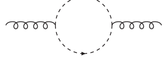
  Figure 1: Diagram relevant for the gauge boson polarization.

• A third point of interest is the modified infrared behaviour of the propagators due to the non-vanishing condensates. If one considers the Landau gauge, the Kugo-Ojima confinement criterion [41] can be translated into an infrared enhancement of the ghost propagator, i.e. the ghost propagator should be more singular than $\frac{1}{p^{2}}$ [58]. Recently, much effort has been paid to investigate this criterion (in the Landau gauge) by means of the Schwinger-Dyson equations, see e.g. [59, 60, 61, 62, 63, 64] and references therein. Defining the gluon and ghost form factors from the Euclidean propagators $D_{\mu\nu}(p^{2})$ and $G(p^{2})$ as

  $$D_{\mu\nu}(p^{2}) = \left(\delta_{\mu\nu}-\frac{p_{\mu}p_{\nu}}{p^{2}}\right)\frac{Z_{D}(p^{2})}{p^{2}}$$

  $$G(p^{2}) = \frac{Z_{G}(p^{2})}{p^{2}}$$ (6.2)

  it was shown that in the infrared

  $$Z_{D}(p^{2}) \sim (p^{2})^{2a}$$

  $$Z_{G}(p^{2}) \sim (p^{2})^{-a}$$ (6.3)

  with $a\approx 0.595$ [60, 61, 62, 63]. As such, the obtained solutions of the Schwinger-Dyson equations seem to be compatible with the Kugo-Ojima confinement criterion. Furthermore, these solutions were also in qualitative agreement with the lattice behaviour (see e.g. [60]). It would be instructive to investigate to what extent the Schwinger-Dyson solutions are modified if one would work with the Landau gauge action

  $$S = S_{YM}+S_{GF+FP}+\int d^{4}x\left(-\frac{\varphi^{2}}{2g^{2}\xi}-\frac{\sigma^{a}\overline{\sigma}^{a}}{g^{2}\zeta}-\frac{\phi^{a}\phi^{a}}{2g^{2}\rho}\right.$$ (6.4)

  $$+ \left.\frac{\varphi}{2g\xi}A_{\mu}^{a}A^{\mu a}+\frac{\overline{\sigma}^{a}}{2g\zeta}gf^{abc}c^{b}c^{c}-\frac{\sigma^{a}}{2g\zeta}gf^{abc}\overline{c}^{b}\overline{c}^{c}-\frac{\phi^{a}}{g\rho}gf^{abc}\overline{c}^{b}c^{c}\right.$$

  $$- \left.\frac{1}{8\xi}\left(A_{\mu}^{a}A^{\mu a}\right)^{2}-\frac{1}{2\rho}g^{2}\left(f^{abc}\overline{c}^{b}c^{c}\right)^{2}+\frac{1}{4\zeta}g^{2}f^{abc}c^{b}c^{c}f^{ade}\overline{c}^{d}\overline{c}^{e}\right)$$

  that already incorporates the non-perturbative effects of the ghost condensates and the gluon condensates, thus also a gluon mass.
  
  Very recently, some results for general covariant gauges concerning the ghost-antighost condensate $\left\langle c^{a}\overline{c}^{a}\right\rangle$ were presented in [65] within the Schwinger-Dyson approach. In the used approximation scheme, it turns out that in case of the linear gauges, no ghost-antighost condensate seems to exist. It is worth remarking here that the ghost-antighost condensate $\left\langle c^{a}\overline{c}^{a}\right\rangle$ is not BRST invariant. It can be combined with the gluon operator $A^{2}$ to yield the mixed gluon-ghost dimension two operator $\frac{1}{2}A^{2}+\alpha\overline{c}c$. To our knowledge, this operator is on-shell BRST invariant only in the Curci-Ferrari and in the Maximal Abelian gauge [56, 57, 66]. In particular, concerning the nonlinear Curci-Ferrari gauge, the condensate $\left\langle\frac{1}{2}A^{2}+\alpha\overline{c}c\right\rangle$ has been proven to show up in the weak coupling [40]. However, no definitive conclusion has been reached so far about this condensate within the Schwinger-Dyson framework [65]. Finally, we notice that the ghost operators $f^{abc}c^{b}c^{c},f^{abc}\overline{c}^{b}c^{c}$ and $f^{abc}\overline{c}^{b}\overline{c}^{c}$ we discussed here, were not considered in [65].

• We have discussed the ghost condensation in the Curci-Ferrari gauge. Originally, the ghost condensates came to attention in the Maximal Abelian gauge in [11, 12, 13, 14, 16, 19, 28]. An approach close to the one presented here should be applied to probe the ghost condensates and their consequences in the Maximal Abelian gauge too. However, the Maximal Abelian gauge is a bit more tricky to handle, see e.g. [40] for some more comments on this.

• So far, the gauges where the ghost condensation takes place, all have the $NO$ symmetry. The important question rises if the ghost condensation only takes place in gauges possessing the $NO$ symmetry? In order to do so, one should first investigate if external sources for the ghost operators can be introduced without spoiling the renormalizability. Assuming that the condensation takes place in gauges without the extra $NO$ invariance, we are however no longer able to relate the different channels by a $NO$ transformation. Neither would we be able anymore to define e.g. a ’new’ Faddeev-Popov charge in non-Overhauser like vacua. Therefore, one might speculate that the enlarged symmetry structure of Yang-Mills theory is necessary to make sense out of the theory, at least if the ghost condensation occurs.

7 Conclusion

In this article, we considered Yang-Mills theory in the Curci-Ferrari gauge and as a limiting case, in the Landau gauge. These gauges possess a global continuous symmetry, generated by the $NO$ algebra. This algebra is built out of the (anti-)BRST transformation and of the $SL(2,R)$ algebra. By combining the local composite operator formalism with the algebraic renormalization technique, we have proven that a ghost condensation $\grave{\textrm{a}}$ la $\left\langle f^{abc}c^{b}c^{c}\right\rangle$, $\left\langle f^{abc}\overline{c}^{b}\overline{c}^{c}\right\rangle$ (BCS channel) and $\left\langle f^{abc}\overline{c}^{b}c^{c}\right\rangle$ (Overhauser channel) occurs. It has been shown that different vacua are possible, with the Overhauser and BCS vacuum as two special choices. The ghost condensates (partially) break the $NO$ symmetry. We have discussed the BRST and the ghost number symmetry in the condensed vacua. We paid attention to the global $SU(N)$ color symmetry and to the absence of Goldstone bosons in the physical spectrum. We also briefly discussed the generalization to the case when quark fields are included. We ended with some comments on future research.

8 Appendix A

8.1 Ward identities for the $NO$ algebra in the Curci-Ferrari gauge

The renormalizability of the Curci-Ferrari gauge is well established [25, 47, 57]. In this Appendix we show that the introduction of a suitable set of external sources allows to write down Ward identities for all the generators of the $NO$ algebra. In particular, these Ward identities will imply that all ghost polynomials $f^{abc}c^{b}c^{c}$, $f^{abc}\overline{c}^{b}\overline{c}^{c}$, $f^{abc}\overline{c}^{b}c^{c}$ have the same anomalous dimension.

In order to write down the functional identities for the $NO$ algebra, we need to introduce three more external sources $\Omega_{\mu}^{a}$, $\overline{\Omega}_{\mu}^{a}$, $\vartheta_{\mu}^{a}$ with dimensions $\left(2,2,1\right)$, coupled to the nonlinear BRST and anti-BRST variations of the gauge field $A_{\mu}^{a}$.

$$S_{ext}=s\overline{s}\int d^{4}x\left(\vartheta^{a\mu}A_{\mu}^{a}+\frac{\gamma}{2}\vartheta^{a\mu}\vartheta_{\mu}^{a}\right)$$ (8.1)

Notice that the coefficient $\gamma$ is allowed by power counting, since the term $\vartheta^{a\mu}\vartheta_{\mu}^{a}$ has dimension $2$. The generators of the $NO$ algebra act on $\Omega_{\mu}^{a}$, $\overline{\Omega}_{\mu}^{a}$, $\vartheta_{\mu}^{a}$ as

$$s\vartheta_{\mu}^{a} = \overline{\Omega}_{\mu}^{a}$$ (8.2)

$$s\overline{\Omega}_{\mu}^{a} = s\Omega_{\mu}^{a}=0$$

$$\overline{s}\vartheta_{\mu}^{a} = -\Omega_{\mu}^{a}$$ (8.3)

$$\overline{s}\Omega_{\mu}^{a} = \overline{s}\overline{\Omega}_{\mu}^{a}=0$$

$$\delta\Omega_{\mu}^{a} = -\overline{\Omega}_{\mu}^{a}$$ (8.4)

$$\delta\vartheta_{\mu}^{a} = \delta\Omega_{\mu}^{a}=0$$

and

$$\overline{\delta}\overline{\Omega}_{\mu}^{a} = -\Omega_{\mu}^{a}$$ (8.5)

$$\overline{\delta}\vartheta_{\mu}^{a} = \overline{\delta}\Omega_{\mu}^{a}=0$$

Therefore, for $S_{ext}$ one gets

$$S_{ext}=\int d^{4}x\left(-\Omega^{\mu a}D_{\mu}^{ab}c^{b}-\overline{\Omega}^{\mu a}D_{\mu}^{ab}\overline{c}^{b}+\gamma\Omega^{\mu a}\overline{\Omega}_{\mu}^{a}-\vartheta^{a\mu}D_{\mu}^{ab}b^{b}+gf^{abc}\vartheta^{a\mu}\left(D_{\mu}^{bd}c^{d}\right)\overline{c}^{c}\right)$$ (8.6)

¿From this expression, it can be seen that the parameter $\gamma$ is needed to account for the behavior of the two-point Green function $\left\langle\left(D_{\mu}^{ab}c^{b}(x)\right)\left(D_{\nu}^{cd}\overline{c}^{d}(y)\right)\right\rangle$, which is deeply related to the Kugo-Ojima criterion. In other words, the coefficient $\gamma$ is the LCO parameter for this Green function.

We can now translate the whole $NO$ algebra into functional identities, which will be the starting point for the algebraic characterization of the allowed counterterm. It turns out thus that, in the Curci-Ferrari gauge, the complete action $\Sigma$

$$\Sigma = S_{YM}+S_{GF+FP}+S_{LCO}+S_{ext}$$ (8.7)

$$= -\frac{1}{4}\int d^{4}xF_{\mu\nu}^{a}F^{a\mu\nu}+s\overline{s}\int d^{4}x\left(\frac{}{}\lambda^{a}c^{a}+\zeta\lambda^{a}\eta^{a}+\eta^{a}\overline{c}^{a}\right.$$

$$\left.\,\,\,\,\,\,\,\,\,\,\,\,\,\,\,\,\,\,\,\,\,\,\,\,-\frac{\alpha}{2}c^{a}\overline{c}^{a}+\vartheta^{a\mu}A_{\mu}^{a}+\frac{1}{2}A_{\mu}^{a}A^{a\mu}+\frac{\gamma}{2}\vartheta^{a\mu}\vartheta_{\mu}^{a}\right)$$

is constrained by the following identities:

• the Slavnov-Taylor identity

  $$\mathcal{S}(\Sigma)=0$$ (8.8)

  $$\mathcal{S}(\Sigma) = \int d^{4}x\left(\left(\frac{\delta\Sigma}{\delta\Omega^{a\mu}}-\gamma\overline{\Omega}_{\mu}^{a}\right)\frac{\delta\Sigma}{\delta A_{\mu}^{a}}+\left(\frac{\delta\Sigma}{\delta L^{a}}-\zeta\tau^{a}\right)\frac{\delta\Sigma}{\delta c^{a}}\right.$$ (8.9)

  $$\;\;\;\;\;\;\;\;\;\left.+b^{a}\frac{\delta\Sigma}{\delta\overline{c}^{a}}+\tau^{a}\frac{\delta\Sigma}{\delta\eta^{a}}+\omega^{a}\frac{\delta\Sigma}{\delta\lambda^{a}}+\overline{\Omega}_{\mu}^{a}\frac{\delta\Sigma}{\delta\vartheta_{\mu}^{a}}\right)$$

• the anti-Slavnov-Taylor identity

  $$\overline{\mathcal{S}}(\Sigma)=0$$ (8.10)

  $$\overline{\mathcal{S}}(\Sigma) = \int d^{4}x\left(\left(\frac{\delta\Sigma}{\delta\overline{\Omega}^{a\mu}}+\gamma\Omega_{\mu}^{a}\right)\frac{\delta\Sigma}{\delta A_{\mu}^{a}}-\left(\frac{\delta\Sigma}{\delta\tau^{a}}-\zeta L^{a}\right)\frac{\delta\Sigma}{\delta\overline{c}^{a}}\right.\;$$ (8.11)

  $$\;\;\;\;\;\left.-\left(b^{a}+\frac{\delta\Sigma}{\delta\omega^{a}}-2\zeta\omega^{a}\right)\frac{\delta\Sigma}{\delta c^{a}}-\frac{\delta\Sigma}{\delta\eta^{a}}\frac{\delta\Sigma}{\delta b^{a}}+L^{a}\frac{\delta\Sigma}{\delta\lambda^{a}}\right.$$

  $$\;\;\;\;\;\left.-\omega^{a}\frac{\delta\Sigma}{\delta\eta^{a}}-\Omega^{a\mu}\frac{\delta\Sigma}{\delta\vartheta^{a\mu}}\right)$$

• the $\delta$ Ward identity

  $$\mathcal{W}(\Sigma)=0$$ (8.12)

  with

  $$\mathcal{W}(\Sigma) = \int d^{4}x\left(c^{a}\frac{\delta\Sigma}{\delta\overline{c}^{a}}+\left(\frac{\delta\Sigma}{\delta L^{a}}-\zeta\tau^{a}\right)\frac{\delta\Sigma}{\delta b^{a}}+2\omega^{a}\frac{\delta\Sigma}{\delta L^{a}}\right.\;$$ (8.13)

  $$\;\;\;\;\;\;\;\;\left.-\tau^{a}\frac{\delta\Sigma}{\delta\omega^{a}}-\eta^{a}\frac{\delta\Sigma}{\delta\lambda^{a}}-\overline{\Omega}_{\mu}^{a}\frac{\delta\Sigma}{\delta\Omega_{\mu}^{a}}\right)$$

• the $\overline{\delta}$ Ward identity

  $$\overline{\mathcal{W}}(\Sigma)=0$$ (8.14)

  $$\overline{\mathcal{W}}(\Sigma) = \int d^{4}x\left(\overline{c}^{a}\frac{\delta\Sigma}{\delta c^{a}}-\left(\frac{\delta\Sigma}{\delta\tau^{a}}-\zeta L^{a}\right)\frac{\delta\Sigma}{\delta b^{a}}-2\omega^{a}\frac{\delta\Sigma}{\delta\tau^{a}}\right.\;$$ (8.15)

  $$\;\;\;\;\;\;\;\;\left.+L^{a}\frac{\delta\Sigma}{\delta\omega^{a}}-\lambda^{a}\frac{\delta\Sigma}{\delta\eta^{a}}-\Omega_{\mu}^{a}\frac{\delta\Sigma}{\delta\overline{\Omega}_{\mu}^{a}}\right)$$

8.2 Algebraic characterization of the invariant counterterm in the Curci-Ferrari gauge

The most general local invariant counterterm compatible with both Slavnov-Taylor and anti-Slavnov-Taylor identities $\left(\mathrm{{\ref{stl}}}\right)$, $\left(\mathrm{{\ref{ast}}}\right)$ can be written as

$$\Sigma^{c} = -\frac{\sigma}{4}\int d^{4}xF_{\mu\nu}^{a}F^{a\mu\nu}+\mathcal{B}\overline{\mathcal{B}}\int d^{4}x\left(\frac{}{}a_{1}\lambda^{a}c^{a}+a_{2}\eta^{a}\lambda^{a}+a_{3}\eta^{a}\overline{c}^{a}\right.$$ (8.16)

$$\left.\,\,\,\,\,\,\,\,\,\,\,\,\,\,\,\,\,\,\,\,\,\,\,\,+\frac{a_{4}}{2}c^{a}\overline{c}^{a}+a_{5}\vartheta_{\mu}^{a}A^{a\mu}+\frac{a_{6}}{2}A^{a\mu}A_{\mu}^{a}+\frac{a_{7}}{2}\vartheta_{\mu}^{a}\vartheta^{a\mu}\right)$$

where $\sigma$, $a_{1}$, $a_{2}$, $a_{3}$, $a_{4}$, $a_{5}$, $a_{6}$, $a_{7}$ are free parameters and $\mathcal{B}$, $\overline{\mathcal{B}}$ denote the linearized nilpotent operators

$$\mathcal{B} = \int d^{4}x\left(\frac{\delta\Sigma}{\delta A_{\mu}^{a}}\frac{\delta}{\delta\Omega^{a\mu}}+\left(\frac{\delta\Sigma}{\delta\Omega^{a\mu}}-\gamma\overline{\Omega}_{\mu}^{a}\right)\frac{\delta}{\delta A_{\mu}^{a}}+\left(\frac{\delta\Sigma}{\delta L^{a}}-\zeta\tau^{a}\right)\frac{\delta}{\delta c^{a}}\right.$$ (8.17)

$$\;\;\;\;\;\;\;\;\;\;\left.+\frac{\delta\Sigma}{\delta c^{a}}\frac{\delta}{\delta L^{a}}+b^{a}\frac{\delta}{\delta\overline{c}^{a}}+\tau^{a}\frac{\delta}{\delta\eta^{a}}+\omega^{a}\frac{\delta}{\delta\lambda^{a}}+\overline{\Omega}_{\mu}^{a}\frac{\delta}{\delta\vartheta_{\mu}^{a}}\right)$$

and

$$\overline{\mathcal{B}} = \int d^{4}x\left(\frac{\delta\Sigma}{\delta A_{\mu}^{a}}\frac{\delta}{\delta\overline{\Omega}_{\mu}^{a}}+\left(\frac{\delta\Sigma}{\delta\overline{\Omega}^{a\mu}}+\gamma\Omega_{\mu}^{a}\right)\frac{\delta}{\delta A_{\mu}^{a}}-\left(\frac{\delta\Sigma}{\delta\tau^{a}}-\zeta L^{a}\right)\frac{\delta}{\delta\overline{c}^{a}}-\frac{\delta\Sigma}{\delta\overline{c}^{a}}\frac{\delta}{\delta\tau^{a}}\right.$$ (8.18)

$$\left.-\left(b^{a}+\frac{\delta\Sigma}{\delta\omega^{a}}-2\zeta\omega^{a}\right)\frac{\delta}{\delta c^{a}}-\frac{\delta\Sigma}{\delta c^{a}}\frac{\delta}{\delta\omega^{a}}-\frac{\delta\Sigma}{\delta\eta^{a}}\frac{\delta}{\delta b^{a}}-\frac{\delta\Sigma}{\delta b^{a}}\frac{\delta}{\delta\eta^{a}}\right.$$

$$\left.+L^{a}\frac{\delta}{\delta\lambda^{a}}-\omega^{a}\frac{\delta}{\delta\eta^{a}}-\Omega^{a\mu}\frac{\delta}{\delta\vartheta^{a\mu}}\right)$$

¿From the $\delta$ and $\overline{\delta}$ Ward identities $\left(\mathrm{{\ref{dwl}}}\right)$, $\left(\mathrm{{\ref{adid}}}\right)$ it follows that

$$a_{3}=a_{1}$$ (8.19)

so that the final expression for $\left(\mathrm{{\ref{invc}}}\right)$ becomes

$$\Sigma^{c} = -\frac{\sigma}{4}\int d^{4}xF_{\mu\nu}^{a}F^{a\mu\nu}+\mathcal{B}\overline{\mathcal{B}}\int d^{4}x\left(\frac{}{}a_{1}\lambda^{a}c^{a}+a_{2}\eta^{a}\lambda^{a}+a_{1}\eta^{a}\overline{c}^{a}\right.$$ (8.20)

$$\left.\,\,\,\,\,\,\,\,\,\,\,\,\,\,\,\,\,\,\,\,\,\,\,\,\,+\frac{a_{4}}{2}c^{a}\overline{c}^{a}+a_{5}\vartheta_{\mu}^{a}A^{a\mu}+\frac{a_{6}}{2}A^{a\mu}A_{\mu}^{a}+\frac{a_{7}}{2}\vartheta_{\mu}^{a}\vartheta^{a\mu}\right)$$

The coefficients $\sigma$, $a_{1}$, $a_{2}$, $a_{4}$, $a_{5}$, $a_{6}$, $a_{7}$ are easily seen to correspond to a multiplicative renormalization of the coupling constant $g$, of the gauge and LCO parameters $\alpha$, $\zeta$, $\gamma$, of the fields and external sources. In particular, the coefficients $\sigma$ and $a_{5}$ are related to the renormalization of the gauge coupling constant $g$ and of the gauge field $A_{\mu}^{a}$, as it is apparent from

$$\mathcal{B}\overline{\mathcal{B}}\int d^{4}x\vartheta_{\mu}^{a}A^{a\mu}=-\mathcal{N}_{A}\Sigma\,\,\,$$ (8.21)

where $\mathcal{N}_{A}$ stands for the invariant counting operator

$$\mathcal{N}_{A}=\int d^{4}x\left(A_{\mu}^{a}\frac{\delta}{\delta A_{\mu}^{a}}-\Omega_{\mu}^{a}\frac{\delta}{\delta\Omega_{\mu}^{a}}-\overline{\Omega}_{\mu}^{a}\frac{\delta}{\delta\overline{\Omega}_{\mu}^{a}}-\vartheta_{\mu}^{a}\frac{\delta}{\delta\vartheta_{\mu}^{a}}\right)+\gamma\frac{\partial}{\partial\gamma}\,\,\,$$ (8.22)

The coefficient $a_{4}$ corresponds to the renormalization of the gauge parameter $\alpha$, indeed

$$\mathcal{B}\overline{\mathcal{B}}\int d^{4}x\frac{1}{2}c^{a}\overline{c}^{a}=-\frac{\partial\Sigma}{\partial\alpha}$$ (8.23)

The coefficient $a_{2}$ is associated to the renormalization of the LCO parameter $\zeta,$ which follows from

$$\mathcal{B}\overline{\mathcal{B}}\int d^{4}x\eta^{a}\lambda^{a}=-\mathcal{N}_{\zeta}\Sigma$$ (8.24)

with

$$\mathcal{N}_{\zeta}=\zeta\frac{\partial}{\partial\zeta}+\int d^{4}x\left(\omega^{a}\frac{\delta}{\delta b^{a}}-\eta^{a}\frac{\delta}{\delta c^{a}}+\lambda^{a}\frac{\delta}{\delta\overline{c}^{a}}\right)$$ (8.25)

The coefficient $a_{1}$ is related to the anomalous dimensions of all ghost operators, namely

$$\mathcal{B}\overline{\mathcal{B}}\int d^{4}x\left(\lambda^{a}c^{a}+\eta^{a}\overline{c}^{a}\right)=\mathcal{N}_{L}\Sigma$$ (8.26)

where

$$\mathcal{N}_{L} = \;\int d^{4}x\left(L^{a}\frac{\delta}{\delta L^{a}}+\tau^{a}\frac{\delta}{\delta\tau^{a}}+\lambda^{a}\frac{\delta}{\delta\lambda^{a}}+\omega^{a}\frac{\delta}{\delta\omega^{a}}+\eta^{a}\frac{\delta}{\delta\eta^{a}}\right.$$ (8.27)

$$\left.\,\,\,\,\,\,\,\,\,\,\,\,\,\,\,\,\,\,\,\,\,-b^{a}\frac{\delta}{\delta b^{a}}-\overline{c}^{a}\frac{\delta}{\delta\overline{c}^{a}}-c^{a}\frac{\delta}{\delta c^{a}}\right)-2\zeta\frac{\partial}{\partial\zeta}\,\,\,$$

The renormalization of the LCO parameter $\gamma$ is given by the coefficient $a_{7}$, as can be seen from

$$\mathcal{B}\overline{\mathcal{B}}\int d^{4}x\left(\frac{1}{2}\vartheta_{\mu}^{a}\vartheta^{a\mu}\right)=\left(\frac{\partial}{\partial\gamma}-\int d^{4}x\,\vartheta_{\mu}^{a}\frac{\delta}{\delta A_{\mu}^{a}}\right)\Sigma\,\,\,$$ (8.28)

Finally, the anomalous dimension of the ghost $c^{a}\,$and the antighost $\overline{c}^{a}$ are obtained from the coefficient $a_{6}$

$$\mathcal{B}\overline{\mathcal{B}}\int d^{4}x\left(\frac{1}{2}A^{a\mu}A_{\mu}^{a}\right)=\mathcal{N}_{c}\Sigma\,\,\,$$ (8.29)

with

$$\mathcal{N}_{c} = \;\int d^{4}x\left(\frac{1}{2}\,c^{a}\frac{\delta}{\delta c^{a}}+\frac{1}{2}\,\overline{c}^{a}\frac{\delta}{\delta\overline{c}^{a}}+b^{a}\frac{\delta}{\delta b^{a}}-L^{a}\frac{\delta}{\delta L^{a}}-\tau^{a}\frac{\delta}{\delta\tau^{a}}-\omega^{a}\frac{\delta}{\delta\omega^{a}}\right.$$ (8.30)

$$\left.\,\,\,\,\,\,\,\,\,\,\,\,\,\,\,\,\,\,\,\,\,-\frac{3}{2}\lambda^{a}\frac{\delta}{\delta\lambda^{a}}-\frac{3}{2}\eta^{a}\frac{\delta}{\delta\eta^{a}}\right)-2\alpha\frac{\partial}{\partial\alpha}+2\zeta\frac{\partial}{\partial\zeta}\,\,\,$$

¿From expressions $\left(\mathrm{{\ref{nl}}}\right)$ and $\left(\mathrm{{\ref{ncc}}}\right)$ one sees that all sources $L^{a},\tau^{a},$ and $\omega^{a}$ renormalize in the same way, which means that all composite ghost polynomials $f^{abc}c^{b}c^{c}$, $f^{abc}\overline{c}^{b}\overline{c}^{c}$, $f^{abc}\overline{c}^{b}c^{c}$ have indeed the same anomalous dimension. This result is a consequence of the relationship $\left(\mathrm{{\ref{a3a1}}}\right)$ which, of course, stems from the existence of the $NO$ algebra.

9 Appendix B

In order to construct the 1-loop effective potential, we need the values of $\zeta_{0}$, $\rho_{0}$, $\zeta_{1}$ and $\rho_{1}$. These can be calculated as soon we know the divergences proportional to $\omega^{2}$ and $L\tau$ when the generating functional corresponding to the action (3.1) is calculated. In principle, it is sufficient to calculate the divergences proportional to $\omega^{2}$ since the $NO$ invariance leads to $\rho=2\zeta$. Therefore, we can restrict ourselves to the diagrams with only the source $\omega$ connected. Let us write

$$\delta\rho=\delta\rho_{0}g^{2}+\delta\rho_{1}g^{4}+\cdots$$ (9.1)

For $N=2$ and $\alpha=0$, the ghost propagator reads

$$\left\langle\overline{c}^{a}c^{b}\right\rangle_{p}=i\frac{-p^{4}\delta^{ab}+p^{2}g\epsilon^{abc}\omega^{c}-g^{2}\omega^{a}\omega^{b}}{p^{2}\left(p^{4}+g^{2}\omega^{2}\right)}$$ (9.2)

while the gluon propagator is given by

$$\left\langle A_{\mu}^{a}A_{\nu}^{b}\right\rangle_{p}=\frac{-i\delta^{ab}}{p^{2}}\left(g_{\mu\nu}-\frac{p_{\mu}p_{\nu}}{p^{2}}\right)$$ (9.3)

The ghost-antighost-gluon vertex equals

$$g\epsilon^{abc}p_{\mu}$$ (9.4)

The relevant vacuum bubbles are shown in Figure 2.

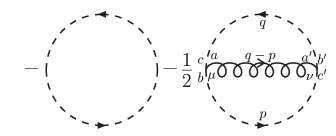
Figure 2: Vacuum bubbles up to 2-loop order, giving divergences proportional to $\omega^{2}$.

At 1-loop, we find a contribution to $\mathcal{W}(\omega,\tau,L)$, given by

$$-i\int\frac{d^{d}p}{(2\pi)^{d}}\ln\left(p^{4}+g^{2}\omega^{2}\right)$$ (9.5)

Performing a Wick rotation and employing the $\overline{MS}$ scheme, this leads to a divergence given by

$$g^{2}\omega^{2}\frac{1}{32\pi^{2}}\frac{4}{\varepsilon}$$ (9.6)

Hence

$$\delta\rho_{0}=-\frac{1}{4\pi^{2}}\frac{1}{\varepsilon}$$ (9.7)

At 2-loops, the contribution to $\mathcal{W}(\omega,\tau,L)$ is obtained by computing the second diagram of Figure 2, yielding

$$\mathcal{I}=\frac{1}{2}ig^{2}\epsilon^{abc}\epsilon^{a^{\prime}b^{\prime}c^{\prime}}\int\frac{d^{d}p}{(2\pi)^{d}}\frac{d^{d}q}{(2\pi)^{d}}\left[p_{\mu}q_{\nu}\frac{-i\delta^{aa^{\prime}}}{(p-q)^{2}}\left(g_{\mu\nu}-\frac{(p-q)_{\mu}(p-q)_{\nu}}{(p-q)^{2}}\right)\right.$$

$$\left.\times i\frac{-p^{4}\delta^{bc^{\prime}}+gp^{2}\epsilon^{bc^{\prime}e}\omega^{e}-g^{2}\omega^{b}\omega^{c^{\prime}}}{p^{2}(p^{4}+g^{2}\omega^{2})}\times i\frac{-q^{4}\delta^{b^{\prime}c}+gq^{2}\epsilon^{b^{\prime}ce}\omega^{e}-g^{2}\omega^{b^{\prime}}\omega^{c}}{q^{2}(q^{4}+g^{2}\omega^{2})}\right]$$ (9.8)

Working out the color algebra, one finds

$$\mathcal{I} = -\frac{g^{2}}{2}\int\frac{d^{d}p}{(2\pi)^{d}}\frac{d^{d}q}{(2\pi)^{d}}\left[\frac{p_{\mu}q_{\nu}}{(p-q)^{2}}\left(g_{\mu\nu}-\frac{(p-q)_{\mu}(p-q)_{\nu}}{(p-q)^{2}}\right)\right.$$ (9.9)

$$\times \left.\frac{-6p^{4}q^{4}-2g^{2}\omega^{2}(p^{4}+q^{4}-p^{2}q^{2})}{p^{2}q^{2}(p^{4}+g^{2}\omega^{2})(q^{4}+g^{2}\omega^{2})}\right]$$

This integral $\mathcal{I}$ has been calculated in two steps: first all tensor integrals have been reduced to a combination of scalar master integrals, applying simple algebraic rearrangements of the scalar products which appear in the numerator of the integrand; all master integrals are vacuum integrals, i.e. with vanishing external momentum; they have been replaced by their explicit expression in terms of special functions [67] and expanded in powers of $\varepsilon$. The calculation has been done with the Mathematica packages DiagExpand and ProcessDiagram. We find

$$\mathcal{I}=\frac{g^{4}\omega^{2}}{(16\pi^{2})^{2}}\left(\frac{6}{\varepsilon^{2}}+\frac{17}{2\varepsilon}-\frac{6}{\varepsilon}\ln\frac{g\omega}{\overline{\mu}^{2}}+\textrm{finite}\right)$$ (9.10)

We also have to take the counterterm information into account. Since there is no counterterm $\propto\omega^{a}gf^{abc}\overline{c}^{b}c^{c}$ in the Landau gauge, the only counterterm that will contribute at the order we are working, is

$$\delta Z_{c}\overline{c}^{a}\partial_{\mu}\partial^{\mu}\delta^{ab}c^{b}$$ (9.11)

where [47]

$$\delta Z_{c}=\frac{3}{2}\frac{g^{2}N}{16\pi^{2}}\frac{1}{\varepsilon}+\cdots\equiv z_{c}^{1}g^{2}+\cdots$$ (9.12)

This leads to a contribution

$$\left(-2z_{c}^{1}g^{2}\right)\left(-i\int\frac{d^{d}p}{(2\pi)^{d}}\ln\left(p^{4}+g^{2}\omega^{2}\right)\right)$$ (9.13)

Or

$$\left[-2z_{c}^{1}g^{2}\right]\left[-\frac{g^{2}\omega^{2}}{32\pi^{2}}\left(-\frac{4}{\varepsilon}+2\ln\frac{g\omega}{\overline{\mu}^{2}}-3\right)\right]=\frac{g^{4}\omega^{2}}{(16\pi^{2})^{2}}\left(-\frac{12}{\varepsilon^{2}}-\frac{9}{\varepsilon}+\frac{6}{\varepsilon}\ln\frac{g\omega}{\overline{\mu}^{2}}+\textrm{finite}\right)$$ (9.14)

Hence, the complete 2-loop contribution to $\mathcal{W}(\omega,\tau,L)$ yields

$$(\ref{mi})+(\ref{tata})=\frac{g^{4}\omega^{2}}{(16\pi^{2})^{2}}\left(-\frac{6}{\varepsilon^{2}}-\frac{1}{2\varepsilon}+\textrm{finite}\right)$$ (9.15)

A good internal check of the calculations is that the terms proportional to $\frac{1}{\varepsilon}\ln\frac{g\omega}{\overline{\mu}^{2}}$ are cancelled. Finally, we find that

$$\delta\rho_{1}=\frac{1}{\left(16\pi^{2}\right)^{2}}\left(\frac{1}{\varepsilon}+\frac{12}{\varepsilon^{2}}\right)$$ (9.16)

References

• [1] F. V. Gubarev, L. Stodolsky and V. I. Zakharov, Phys. Rev. Lett. 86 (2001) 2220
• [2] F. V. Gubarev and V. I. Zakharov, Phys. Lett. B 501 (2001) 28
• [3] P. Boucaud, G. Burgio, F. Di Renzo, J. P. Leroy, J. Micheli, C.  Parrinello, O. P$\grave{\textrm{e}}$ne, C. Pittori, J. Rodriguez-Quintero, C. Roiesnel and K. Sharkey, JHEP 0004 (2000) 006
• [4] P. Boucaud, A. Le Yaouanc, J. P. Leroy, J. Micheli, O. P$\grave{\textrm{e}}$ne and J. Rodriguez-Quintero, Phys. Rev. D 63 (2001) 114003
• [5] P. Boucaud, J. P. Leroy, A. Le Yaouanc, J. Micheli, O. Pène, F.  De Soto, A. Donini, H. Moutarde and J. Rodriguez-Quintero, Phys. Rev. D 66 (2002) 034504
• [6] H. Verschelde, K. Knecht, K. Van Acoleyen and M. Vanderkelen, Phys. Lett. B 516 (2001) 307, Erratum-ibid., to appear
• [7] M. A. Semenov-Tyan-Shanskii and V. A. Franke, Zapiski Nauchnykh Sem. Leningradskogo Otdeleniya Mat. Inst. im. V.A. Steklov AN SSSR 120, 159 (1982). Translation (Plenum, New York, 1986) 1999
• [8] D. Zwanziger, Nucl. Phys. B 345 (1990) 461
• [9] L. Stodolsky, P. van Baal and V. I. Zakharov, Phys. Lett. B 552 (2003) 214
• [10] D. Dudal, A. R. Fazio, V. E. Lemes, M. Picariello, M. S. Sarandy, S. P. Sorella and H. Verschelde, Vacuum Condensates of Dimension Two in Pure Euclidean Yang-Mills, hep-th/0304249
• [11] M. Schaden, Mass generation in continuum SU(2) gauge theory in covariant Abelian gauges, hep-th/9909011
• [12] M. Schaden, SU(2) gauge theory in covariant (maximal) Abelian gauges, hep-th/0003030
• [13] M. Schaden, Mass generation, ghost condensation and broken symmetry: SU(2) in covariant Abelian gauges, hep-th/0108034
• [14] K. I. Kondo and T. Shinohara, Phys. Lett. B 491 (2000) 263
• [15] D. J. Gross and A. Neveu, Phys. Rev. D 10 (1974) 3235
• [16] D. Dudal and H. Verschelde, On ghost condensation, mass generation and Abelian dominance in the maximal Abelian gauge, hep-th/0209025
• [17] H. Verschelde, S. Schelstraete and M. Vanderkelen, Z. Phys. C 76 (1997) 161
• [18] C. Luperini and P. Rossi, Annals Phys.  212 (1991) 371
• [19] V. E. Lemes, M. S. Sarandy and S. P. Sorella, Ghost number dynamical symmetry breaking in Yang-Mills theories in the maximal Abelian gauge, hep-th/0206251
• [20] J. Bardeen, L. N. Cooper and J. R. Schrieffer, Phys. Rev.  106 (1957) 162
• [21] J. Bardeen, L. N. Cooper and J. R. Schrieffer, Phys. Rev.  108 (1957) 1175
• [22] A. W. Overhauser, Advances in Physics 27 (1978) 343
• [23] B. Y. Park, M. Rho, A. Wirzba and I. Zahed, Phys. Rev. D 62 (2000) 034015
• [24] R. Delbourgo and P. D. Jarvis, J. Phys. A 15 (1982) 611
• [25] L. Baulieu and J. Thierry-Mieg, Nucl. Phys. B 197 (1982) 477
• [26] G. Curci and R. Ferrari, Nuovo Cim. A 32 (1976) 151
• [27] G. Curci and R. Ferrari, Phys. Lett. B 63 (1976) 91
• [28] V. E. Lemes, M. S. Sarandy, S. P. Sorella, M. Picariello and A. R. Fazio, Mod. Phys. Lett. A 18 (2003) 711
• [29] V. E. Lemes, M. S. Sarandy and S. P. Sorella, hep-th/0210077, Annals Phys., to appear
• [30] K. Knecht and H. Verschelde, Phys. Rev. D 64 (2001) 085006
• [31] O. Piguet and S. P. Sorella, Algebraic Renormalization, Monograph series m28, Springer Verlag, 1995
• [32] G. Barnich, F. Brandt and M. Henneaux, Phys. Rept.  338 (2000) 439
• [33] N. Nakanishi and I. Ojima, Z. Phys. C 6 (1980) 155, Erratum-ibid. C 8 (1981) 94
• [34] F. Delduc and S. P. Sorella, Phys. Lett. B 231 (1989) 408
• [35] H. Sawayanagi, Prog. Theor. Phys.  106 (2001) 971
• [36] K. Nishijima, Prog. Theor. Phys.  72 (1984) 1214
• [37] K. Nishijima, Prog. Theor. Phys.  73 (1985) 536
• [38] N. Nakanishi and I. Ojima, Covariant Operator Formalism of Gauge Theories and Quantum Gravity, vol. 27 of Lecture Notes in Physics, World Scientific, 1990
• [39] D. Dudal, H. Verschelde, V. E. Lemes, M. S. Sarandy, S. P. Sorella and M. Picariello, JHEP 0212 (2002) 008
• [40] D. Dudal, H. Verschelde, V. E. Lemes, M. S. Sarandy, S. P. Sorella and M. Picariello, Gluon-ghost condensate of mass dimension 2 in the Curci-Ferrari gauge, hep-th/0302168
• [41] T. Kugo and I. Ojima, Prog. Theor. Phys. Suppl.  66 (1979) 1
• [42] D. Dudal, H. Verschelde and S. P. Sorella, Phys. Lett. B 555 (2003) 126
• [43] R. Alkofer and L. von Smekal, Phys. Rept.  353 (2001) 281
• [44] S. R. Coleman and E. Weinberg, Phys. Rev. D 7 (1973) 1888
• [45] R. Jackiw, Phys. Rev. D 9 (1974) 1686
• [46] S. A. Larin and J. A. Vermaseren, Phys. Lett. B 303 (1993) 334
• [47] J. A. Gracey, Phys. Lett. B 552 (2003) 101
• [48] D. Dudal, H. Verschelde, R. E. Browne and J. A. Gracey, A determination of $\left\langle A^{2}\right\rangle$ and the non-perturbative vacuum energy of Yang-Mills theory in the Landau gauge, hep-th/0302128, Phys. Lett. B, to appear.
• [49] K. Langfeld, H. Reinhardt and J. Gattnar, Nucl. Phys. B 621 (2002) 131
• [50] C. Alexandrou, P. de Forcrand and E. Follana, Phys. Rev. D 65 (2002) 114508
• [51] G. Grunberg, Phys. Lett. B 95 (1980) 70 [Erratum-ibid. B 110 (1982) 501]
• [52] G. Grunberg, Phys. Rev. D 29 (1984) 2315
• [53] P. M. Stevenson, Phys. Rev. D 23 (1981) 2916
• [54] K. Van Acoleyen and H. Verschelde, Phys. Rev. D 65 (2002) 085006
• [55] H. Sawayanagi, Phys. Rev. D  67 (2003) 045002
• [56] K. I. Kondo, Phys. Lett. B 514 (2001) 335
• [57] K. I. Kondo, T. Murakami, T. Shinohara and T. Imai, Phys. Rev. D 65 (2002) 085034
• [58] T. Kugo, The Universal Renormalization Factors $\frac{Z_{1}}{Z_{3}}$ and Color Confinement Condition in Non-Abelian Gauge Theory, hep-th/9511033
• [59] P. Watson and R. Alkofer, Phys. Rev. Lett.  86 (2001) 5239
• [60] R. Alkofer, C. S. Fischer and L. von Smekal, Kugo-Ojima confinement and QCD Green’s functions in covariant gauges, nucl-th/0301048
• [61] C. Lerche and L. von Smekal, Phys. Rev. D 65 (2002) 125006
• [62] D. Zwanziger, Phys. Rev. D 65 (2002) 094039
• [63] K. Langfeld, Vortex induced confinement and the Kugo-Ojima confinement criterion, hep-lat/0204025
• [64] K. I. Kondo, Implications of analyticity to mass gap, color confinement and infrared fixed point in Yang-Mills theory, hep-th/0303251
• [65] R. Alkofer, C. S. Fischer, H. Reinhardt and L. von Smekal, On the infrared behaviour of gluons and ghosts in ghost-antighost symmetric gauges, hep-th/0304134
• [66] B. M. Gripaios, Phys. Lett. B 558 (2003) 250
• [67] A. I. Davydychev and J. B. Tausk, Nucl. Phys. B 397 (1993) 123