More on core instabilities of magnetic monopoles

Abstract

In this paper we present new results on the core instability of the ’t Hooft Polyakov monopoles we reported on before. This instability, where the spherical core decays in a toroidal one, typically occurs in models in which charge conjugation is gauged. In this paper we also discuss a third conceivable configuration denoted as “split core”, which brings us to some details of the numerical methods we employed. We argue that a core instability of ’t Hooft Polyakov type monopoles is quite a generic feature of models with charged Higgs particles.

1 Introduction

Since the pioneering work of ’t Hooft and Polyakov [1, 2] magnetic monopoles have been studied in detail in many different models. In this paper we report on the results of investigations following our earlier work [3] on the core instability of the fundamental spherically symmetric magnetic monopole solution. We determine the regions in parameter space where this instability occurs and present some details of the numerical simulations we performed. In [3] it was shown that in a rather simple model the spherically magnetic monopole solution is not the global minimal energy solution for all values of the parameters of the model. The fact that the core topology is not fixed by the boundary conditions at infinity and different core topologies can be deformed into each other was already established earlier [4]. As we will indicate, alice theories have a special topological feature which makes it plausible that such a core deformation really can be favored energetically. We will also argue that a core deformation is typically energetically favored in models where the charged Higgs particles are light compared to the neutral Higgs.

This paper is organized as follows. We start with a brief recap of alice electrodynamics (AED) and its features which lead us to expect the core meta-/instability of the monopole. Next we introduce the specific model and discuss in some detail the numerical simulations we performed and present our the main results. We end the paper with conclusions and an outlook.

2 Alice electrodynamics

Alice electrodynamics (AED) is a gauge theory with gauge group $H=U(1)\ltimes\mathbb{Z}_{2}\sim O(2)$, in a certain sense the minimally non-abelian extension of ordinary electrodynamics. The nontrivial $\mathbb{Z}_{2}$ transformation reverses the direction of the electric and magnetic fields and the sign of the charges. In other words, alice electrodynamics is a theory in which charge conjugation symmetry is gauged. However, as this non-abelian extension is discrete, it only affects electrodynamics through certain global (topological) features, such as the appearance of alice fluxes and cheshire charges [5, 6]. In this paper the cheshire phenomenon is of great importance to us as it supports the possible core meta-/instability of the spherically symmetric magnetic monopole solution. The topological structure of $U(1)\ltimes\mathbb{Z}_{2}$ differs from that of $U(1)$ in a few subtle points. AED allows topologically stable localized fluxes since $\Pi_{0}(U(1)\ltimes\mathbb{Z}_{2})=\mathbb{Z}_{2}$, the so called alice fluxes. Note that in this theory this flux is coëxisting with the unbroken $U(1)$ of electromagnetism and is therefore not an ordinary “magnetic” flux. Just as a $U(1)$ gauge theory, AED may contain magnetic monopoles, which follows from the fact that $\Pi_{1}(U(1)\ltimes\mathbb{Z}_{2})=\mathbb{Z}$. We note however, that due to the fact that the $\mathbb{Z}_{2}$ and the $U(1)$ part of the gauge group do not commute, magnetic charges of opposite sign belong to the same topological sector.

It was pointed out long ago that there are interesting issues concerning the core stability of magnetic monopoles. Fixing the asymptotics of the Higgs field, the core (i.e., the zeros of the Higgs field) may have different topologies, notably that of a “ring” rather than the conventional “point”. These core topologies are cobordant, i.e., they can be smoothly deformed into each other and it is a question of energetics what will be the lowest energy monopole state [4]. In AED such a core deformation would be accompanied by the rather unusual delocalized version of (magnetic) charge, the so called magnetic cheshire charge. Cheshire charge is a key feature of AED and is a general phenomena in field theories with (topologically) stable fluxes which are not elements of the center of the unbroken gauge group.

In the specific AED model we consider the Higgs field is a symmetric tensor, whose vacuum expectation value may be depicted as a bidirectional arrow. The head-tail symmetry of the order parameter reflects the charge conjugation symmetry of the theory. In AED we can “punch a hole” in the spherically symmetric monopole and deform it into an alice ring, this configuration is consistent with the continuity requirement on the order parameter because of its head-tail symmetry. In figure 1 we plotted the two different core regions one expects to find for a magnetic monopole in AED. In this paper we determine in what part of the parameter space of the model the monopole is meta-/unstable and where we expect the spherically symmetric monopole to compete with a magnetically, cheshire charged alice ring. Figure 1(a) represents the spherically symmetric magnetic monopole and figure 1(b) represents the magnetically cheshire charge alice ring. The fact that the core of the defect can really deform into a torus is due to the head-tail symmetry of the Higgs field in the broken phase. We note that Higgs field only rotates over an angle $\pi$ when going around a single flux. This is the hallmark for an alice flux, so the core deformed spherical monopole is in fact an alice ring carrying a magnetic cheshire charge, see also [3].

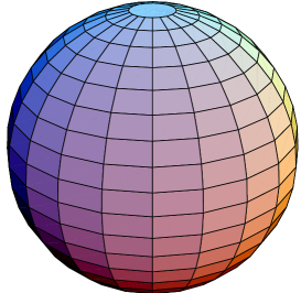
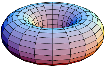
(a) (b)

Figure 1: These figures show the two different core structures of a magnetic defect which are naturally present in AED. Figure (a) represents the spherically symmetric magnetic monopole, the ’t Hooft Polyakov type monopole, and figure (b) represents the magnetically, cheshire charged alice ring.

We just showed that the punctured monopole is a magnetically cheshire charged alice loop. To understand that such a configuration can indeed be stable we make an estimate for the energy of such a charged alice loop. We approximate the energy of the circular alice loop of radius $R$, by $E_{loop}=2\pi R{\cal E}_{flux}$, with ${\cal E}_{flux}$ the energy per unit length of the alice flux, and approximate the energy of the cheshire charge, $E_{ches}$, by a uniformly charged disc with radius $R$. The magnetic field of the latter is given by:

$$\vec{B} = \frac{-Q}{\pi R^{2}}\vec{\nabla}\int_{0}^{1}\int_{0}^{2\pi}\frac{r^{\prime}~{}dr^{\prime}d\theta^{\prime}}{\sqrt{r^{2}+z^{2}+r^{\prime 2}-2rr^{\prime}\cos{\theta^{\prime}}}}$$ (1)

$$\equiv \frac{Q}{R^{2}}~{}\vec{a}(r,z)$$ (2)

Where we have rescaled the coordinates by a factor of $R$ and $Q$ is the total charge. The field energy is then given by:

$$E_{ches} = \int\vec{B}\cdot\vec{B}~{}R^{3}d^{3}x$$ (3)

$$= \frac{Q^{2}}{R}\int\vec{a}(r,z)\cdot\vec{a}(r,z)~{}d^{3}x$$ (4)

$$\equiv \frac{Q^{2}}{R}~{}A$$ (5)

Where $A$ is a dimensionless constant determined by the disc geometry. The total energy of the alice loop of radius $R$, with a cheshire charge $Q$ is thus given by:

$$E_{tot}=2\pi R{\cal E}_{flux}+\frac{Q^{2}}{R}~{}A$$ (6)

As mentioned earlier there are two competing, R-dependent, terms and we may determine the radius of the loop which minimizes the energy, yielding:

$$R=|Q|\sqrt{\frac{A}{2\pi{\cal E}_{flux}}}$$ (7)

Consequently the minimal energy is given by:

$$E=\sqrt{8\pi{\cal E}_{flux}A}~{}|Q|$$ (8)

Obviously this estimate can only be trusted if the radius of the alice loop is much larger than the radius of the alice flux and this should be checked. However this estimate does indicate that the cheshire charged alice loop can be a stable configuration, where the string tension is balanced by the repulsion between the magnetic fieldlines. Interestingly enough this estimate gives an energy proportional to the magnetic charge, $E\propto|Q|$.

3 The model

To answer stability questions related to the spherically symmetric monopole configuration (or the cheshire charged alice ring) we consider an explicit model. We use the original tensor alice model [7], but we could as well have chosen an alternative [8]. We will in fact argue that the results obtained are quite general and model independent. For completeness and notational convenience we briefly summarize the model. The action is given by:

$$S=\int d^{4}x\ \left\{\frac{1}{4}F^{a,\mu\nu}F^{a}_{\mu\nu}+\frac{1}{4}Tr(D^{\mu}\Phi D_{\mu}\Phi)-V(\Phi)\right\}\quad,$$ (9)

where the Higgs field $\Phi=\Phi^{ab}$ is a real, symmetric, traceless $3\times 3$ matrix, i.e., $\Phi$ is in the five dimensional representation of $SO(3)$ and $D_{\mu}\Phi=\partial_{\mu}\Phi-ie[A_{\mu},\Phi]$, with $A_{\mu}=A^{a}_{\mu}T_{a}$, where $T_{a}$ are the generators of $SO(3)$. The most general renormalizeable potential is given by [9]:

$$V=-\frac{1}{2}\mu^{2}Tr\left(\Phi^{2}\right)-\frac{1}{3}\gamma Tr\left(\Phi^{3}\right)+\frac{1}{4}\lambda\left(Tr\left(\Phi^{2}\right)\right)^{2}\quad,$$ (10)

with the parameter $\gamma>0$, since $(\Phi,\gamma)=(-\Phi,-\gamma)$. For a suitable range of the parameters in the potential, the gauge symmetry of the model will be broken to the symmetry of AED. In the “unitary” gauge, where the Higgs field is diagonal, the ground state is (up to permutations) given by the following matrix:

$$\Phi_{0}=\left(\begin{array}[]{ccc}-f&0&0\\ 0&-f&0\\ 0&0&2f\end{array}\right)\quad,$$ (11)

with $f=\frac{\gamma}{12\lambda}\left(1+\sqrt{1+\frac{24\mu^{2}\lambda}{\gamma^{2}}}\right)$.

The full action has four parameters, $e,\mu^{2},\gamma,\lambda$, this number can be reduced to two dimensionless parameters by appropriate rescalings of the variables. A physical choice for these dimensionless parameters is to take the ratio’s of the masses that one finds from perturbing around the homogeneous minimum. To determine these, we write the action in the unitary gauge where the massless components of $\Phi$ have been absorbed by the gauge fields. The physical components of the Higgs field may be expanded as:

$$\Phi(x^{\mu})=\Phi_{0}+\sqrt{2}\phi_{1}(x^{\mu})E_{1}+\sqrt{2}\phi_{2}(x^{\mu})~{}R_{3}(a(x^{\mu}))E_{2}R_{3}(a(x^{\mu}))^{T}\quad,$$ (12)

with:

$$E_{1}=\frac{1}{\sqrt{6}}\left(\begin{array}[]{ccc}-1&0&0\\ 0&-1&0\\ 0&0&2\end{array}\right)~{};~{}~{}E_{2}=\frac{1}{\sqrt{2}}\left(\begin{array}[]{ccc}1&0&0\\ 0&-1&0\\ 0&0&0\end{array}\right)~{};~{}~{}E_{3}=\frac{1}{\sqrt{2}}\left(\begin{array}[]{ccc}0&0&1\\ 0&0&0\\ 1&0&0\end{array}\right)$$ (13)

and $R_{i}$ are the usual rotation matrices. To second order, the potential $V(\Phi)$ takes the following form:

$$V(\Phi)=const.+(2\mu^{2}+\gamma f)\phi_{1}^{2}+3\gamma f|\phi_{2}|^{2}+~{}\cdots\quad,$$ (14)

yielding the two distinct masses of the Higgs modes. Next we look at the ’kinetic’ term, $\frac{1}{4}Tr(D^{\mu}\Phi D_{\mu}\Phi)$, of the Higgs field. Inserting the previous expressions for the Higgs field, we find:

$$\frac{1}{4}Tr(D^{\mu}\Phi D_{\mu}\Phi)=\frac{1}{2}(\partial_{\mu}\phi_{1})^{2}+\frac{1}{2}\left|D_{\mu}^{3}\phi_{2}\right|^{2}+\frac{9}{2}e^{2}f^{2}\left[\left(A_{\mu}^{1}\right)^{2}+\left(A_{\mu}^{2}\right)^{2}\right]+~{}\cdots\quad,$$ (15)

with: $D_{\mu}^{3}=\partial_{\mu}-i2eA^{3}_{\mu}$. The second term shows that the $\phi_{2}$ component of the Higgs field carries a charge $2e$ with respect to the unbroken $U(1)$ component $A_{\mu}^{3}$ of the gauge field. The first term describes the usual charge neutral Higgs particle and the third term yields the mass of the charged gauge fields. So the relevant lowest order action is given by:

$$S=\int d^{4}x\left\{\frac{1}{4}F_{\mu\nu}^{a}F^{a,\mu\nu}+\frac{1}{2}(\partial_{\mu}\phi_{1})^{2}+\frac{1}{2}\left|D_{\mu}^{3}\phi_{2}\right|^{2}-\frac{1}{2}m_{1}^{2}\phi_{1}^{2}\right.$$ (16)

$$\left.-\frac{1}{2}m_{2}^{2}|\phi_{2}|^{2}-\frac{1}{2}m_{A}^{2}\left[\left(A_{\mu}^{1}\right)^{2}+\left(A_{\mu}^{2}\right)^{2}\right]+~{}\cdots\right\}\quad,$$

with $m_{1}^{2}=4\mu^{2}+2\gamma f$, $m_{2}^{2}=6\gamma f$ and $m_{A}^{2}=9e^{2}f^{2}$.

Two degrees of freedom of the five dimensional Higgs field are ’eaten’ by the broken gauge fields, one degree of freedom forms the real neutral scalar field and two degrees of freedom form the complex (doubly charged) scalar field. To specify a point in the classical parameter space we may, up to irrelevant rescalings, use the dimensionless mass ratio’s $\frac{m_{1}}{m_{2}}$ and $\frac{m_{A}}{m_{2}}$. We note that the value of $\frac{m_{1}}{m_{2}}$ needs to be larger or equal to $\frac{1}{3}$, because for smaller values of $\frac{1}{3}$ the groundstate corresponds to the symmetric unbroken vacuum. Note that we found three mass scales in this problem. For the simulations, which we will describe in the next section, this means that we will we have to deal with three different length scales.

4 Numerical simulations

In this section we will describe in some detail the numerical simulations we performed to determine the instability and the meta-stability regions for the spherically symmetric monopole, in the parameter space of the model. First though, we introduce the ansatz. We end the section with the discussion of a typical set of numerical experiments.

4.1 The variational ansatz

As mentioned before we will use a variational approach. In such an approach the configurations one finds are typically not exact solutions to the equations of motion. However as the ansatz we will use contains the ansatz for the exact spherically symmetric solution we may still study the instability and the meta-stability of this solution. This means that the instability and the meta-stability regions we will find for the monopole, are lower bounds, in the sense that those instability regions can only become larger as the ansatz becomes less restrictive.

As we expect the competing configuration of the spherically symmetric magnetic monopole to be the magnetically cheshire charged alice ring, we base our ansatz on cylindrical symmetry, also see [3]. The ansatz we will use also has a reflection symmetry with respect to the $z$$=$$0$-plane. We impose this reflection symmetry to eliminate the (almost) zero mode in the energy due to the position of the defect along the $z$-axis. The ansatz for the Higgs field is:

$$\Phi(z,\rho,\theta=0)=\phi_{1}(z,\rho)E_{1}+\phi_{2}(z,\rho)E_{2}+\phi_{3}(z,\rho)E_{3}$$ (17)

and

$$\Phi(z,\rho,\theta)=R_{3}(\theta)\Phi(z,\rho,\theta=0)R_{3}(\theta)^{T}\quad.$$ (18)

The ansatz for the gauge fields is simply given by $eA_{i}^{j}=-\epsilon_{ijk}\frac{x^{k}}{x^{2}}A(z,\rho)$, very similar to the one for the spherically symmetric monopole [1], except that we allow $A(z,\rho)$ to depend on $\rho$ and $z$ and not only on $r=\sqrt{\rho^{2}+z^{2}}$. The boundary conditions for $r\to\infty$ are the boundary conditions of the spherically symmetric monopole [7], i.e., $A(z,\rho)$ goes to one and the Higgs field to $\Phi(z,\rho,\theta)=R_{3}(\theta)R_{2}\left(\arccos\left(\frac{z}{r}\right)\right)\Phi_{0}R_{2}\left(\arccos\left(\frac{z}{r}\right)\right)^{T}R_{3}(\theta)^{T}$. The boundary conditions at $\rho=0$ and $z=0$ follow by imposing the cylindrical and reflection symmetry and are given in the table below:

$$\begin{array}[]{|c||c|c|}\hline\cr&\rho=0&z=0\\ \hline\cr\phi_{1}&\partial_{\rho}\phi_{1}=0&\partial_{z}\phi_{1}=0\\ \phi_{2}&\partial_{\rho}\phi_{2}=\phi_{2}=0&\partial_{z}\phi_{2}=0\\ \phi_{3}&\phi_{3}=0&\phi_{3}=0\\ A&\partial_{\rho}A=0&\partial_{z}A=0\\ \hline\cr\end{array}$$

It is easy to see that these boundary conditions are also met by the spherically symmetric monopole, so it is indeed contained in our more general ansatz. With the help of this model and ansatz we study the stability of the spherically symmetric magnetic monopole. Before we present the results we describe the numerical methods we employ, and a typical set of experiments.

4.2 Some numerical details

We mentioned in section 3 that the AED model has three mass scales, i.e., three relevant length scales. However we examine a region of parameter space in which only two of those are relevant. That is the core geometry of the defect and the region where the Higgs field is not in the vacuum manifold on the one hand, and the inverse mass of the gauge fields - which is typically much larger - on the other. To be able to adequately capture both scales we use a space and configuration dependent lattice spacing. In fact we will use two types of lattices. In figure 2 we schematically give the step sizes as a function of the point number (in one dimension). The two dimensional lattices we will use have the same type of lattice in both directions.

(a) (b)

Figure 2: The two different types of lattices. The first part covers the core structure of the defects where the second part captures the region where the gauge fields - which have a much smaller mass - show nontrivial behavior. The only difference of a lattice of type (b) with respect to lattice of type (a) is a few extra lattice points near $r=0$ and $z=0$.

The only difference between the two lattices is that in the second, figure 2(b), there are extra lattice points near $r=0$ and $z=0$ and thus it has a more lattice points. However the same part of space is covered by both lattices. Although the difference between the two lattices is quite small we will encounter a specific lattice dependence, which turns out it be an artifact, but nevertheless will be of use later on.

To obtain the minima of the energy within the ansatz for the different values of the parameters of the model, we used a Monte Carlo based cooling method. In this method one introduces a temperature and gives a configuration with energy $E$ a weight factor equal to $e^{-\frac{E}{T}}$. In the limit of $T\to 0$ only the configuration with the lowest energy survives. Assuming there are no flat directions this procedure selects an unique configuration. With the help of a Monte Carlo mechanism different configurations are sampled. We keep sampling at a specific temperature as long as the energy of the system averaged over a preset number of sweeps (typically 10) decreases and do this a minimal number of times (typically 3). When this average energy no longer decreases we lower the temperature (typically by 10%) and repeat the process until the total energy drop at a specific temperature becomes lower then a predetermined relative energy change (typically $\sim 10^{-6}$%). During this process we keep the acceptance rate of the Monte Carlo steps locally fixed for all fields. This means that we introduced a maximum step size for each field at each position and automatically adjust it to get the preferred acceptance rate. Since the change due to temperature change is easy captured we determined the desired maximum step sizes in the beginning of the cooling mechanism and further only correct for the trivial temperature changes, i.e., as $T$ changes in $aT$, $\delta_{field}$ changes in $\sqrt{a}\delta_{field}$. This assumes that the energy change depends quadratically on the field change which is what one naively expects near a stable configuration, and indeed, that criterion worked nicely.

The procedure we just described is used to determine stable configurations within our ansatz for the different values of the parameters of the model. To be able to determine the meta-stability and instability regions of the monopole in the parameter space of the model we perform hysteresis type of experiments. This means that we determine the lowest energy configuration for a specific point in the parameter space and use this configuration as the starting point for the determination of a stable configuration at a point nearby in the parameter space. As the change in the parameter space is only small one would expect the new configuration also to be close to the previous one. We determine the new configuration again with the help of the cooling method. We repeat this process and move along a trajectory in the parameter space and back again. We choose these paths such that the lowest energy configurations on each end of the trajectory are different type of configurations: a spherical monopole and a cheshire charged alice ring. To keep things numerically simple we keep the mass of the gauge fields constant during a hysteresis experiment. This restriction selects specific trajectories in the two dimensional parameter space, which are given by:

$$\frac{m_{A}}{m_{2}}=\frac{2~{}\left(\frac{m_{A}}{m_{2}}\right)_{\frac{1}{3}}}{3\sqrt{\frac{1}{3}+\left(\frac{m_{1}}{m_{2}}\right)^{2}}}\quad,$$ (19)

with $\left(\frac{m_{A}}{m_{2}}\right)_{\frac{1}{3}}$ the value of $\frac{m_{A}}{m_{2}}$ at the minimal value of $\frac{m_{1}}{m_{2}}=\frac{1}{3}$.
This restriction allows us to keep the total space covered by the same lattice throughout the hysteresis. In a single hysteresis experiment the size of the core does not change much, so we keep the lattice fixed throughout a single hysteresis experiment.

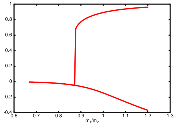
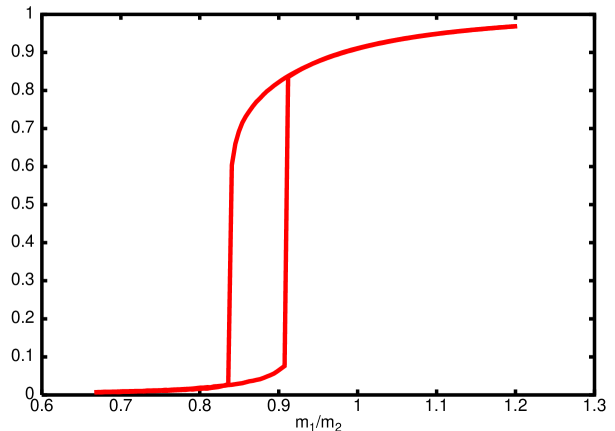
(a) (b)

Figure 3: The two typical results of the hysteresis experiments for the different lattice types projected on the $\frac{m_{1}}{m_{2}}$-axis. Figure (a) corresponds to a lattice of type (a) and figure (b) corresponds to a lattice of type (b).

Figures 3(a) and (b) show the typical hysteresis results. The figures show the values of the field variable $\frac{\phi_{1}}{\sqrt{6}f}$ at $r=z=0$. This variable is a normalized order parameter in the sense that its value equals zero for the spherical monopole, and one for the alice ring. A negative value of the order parameter is also possible and corresponds to a new type of configuration, the so called split core, see figure 4(c) and also [10, 11]. Figure 3(b) shows what one would expect for a hysteresis type of experiment for a lattice of type (b) while figure 3(a) shows a different behavior and corresponds to a lattice of type (a).

In figure 3(a) the split core configuration appears and although this configuration typically has more energy then a cheshire charged alice ring configuration, it does appear to be meta-stable. In [10, 11] this object was discussed for the global analog of AED, a nematic liquid crystal theory, and it was argued that this configuration is due to the cylindrical symmetry restriction of the ansatz used to explore the solution-space. Here we found that it might as well be just a lattice artifact as it depends on the lattice type one uses in the hysteresis experiments. Although this splitcore configuration may be viewed as an undesirable feature caused by lattice and/or symmetry artifacts, we will see that it can be turned into a useful tool.

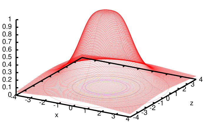
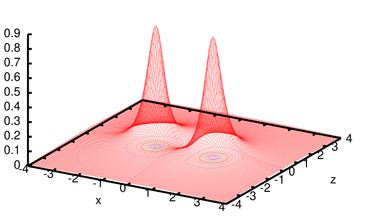
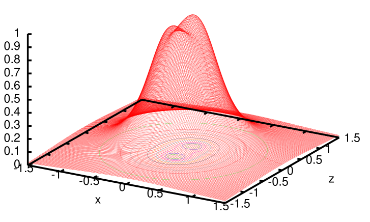
(a) (b) (c)

Figure 4: These figures show the three typical core structures we encountered in the numerical simulations. All three figures show a slice of the core structure at $y=0$ an in the figures the value of $1-\frac{Tr\Phi^{2}}{6f^{2}}$ is plotted. In figure (a) we plotted the core structure of the spherically symmetric magnetic monopole at $\frac{m_{1}}{m_{2}}=0.57$ and $\frac{m_{A}}{m_{2}}=0.0095$. In figure (b) we plotted the core structure of the magnetically cheshire charged alice ring at $\frac{m_{1}}{m_{2}}=0.88$ and $\frac{m_{A}}{m_{2}}=0.0073$ and in figure (c) we plotted the core structure of the split core configuration at $\frac{m_{1}}{m_{2}}=1.12$ and $\frac{m_{A}}{m_{2}}=0.0425$.

4.3 A typical set of experiments

As mentioned before we do hysteresis type of experiments along specific trajectories in the parameter space of the model. Next we look at a typical set of such experiments. We did the hysteresis experiment for three different numbers of lattice points, where we only changed the number of lattice points describing the core of the configuration. One could of course also change the number of points outside the core but we found that that did not make any difference in the observables we examined and did not affect the stability of the configurations. We performed numerical simulations with 25$\times$25 (27$\times$27), 50$\times$50 (54$\times$54) and 100$\times$100 (108$\times$108) lattice points describing the core structure for each line in the parameter space we considered. The figures 5(a-d) are the typical results of such an investigation. The figures show two different observables: the relative energy difference of the two branches of the hysteresis, and the quantity $\frac{\phi_{1}(0,0)}{\sqrt{6}f}$. The figures 5(a) and 5(b) belong to lattices of type (a) and the figures 5(c) and 5(d) belong to lattices of type (b). All figures show the results obtained with the three different number of lattices points, with the lines A, B an C corresponding to 25$\times$25 (27$\times$27), 50$\times$50 (54$\times$54) and 100$\times$100 (108$\times$108) points describing the core structure respectively.

Let us first compare the figures 5(a) and 5(c). These figures show the values of $\frac{\phi_{1}(0,0)}{\sqrt{6}f}$. In both figures we see that qualitatively the lines A, B and C do not differ very much, but quantitatively they do. The steep part of the lines corresponds to the local instability of the cheshire charged alice ring and the spherical monopole. In both figures 5(a) and 5(c) we see that the alice ring becomes locally unstable with respect to the monopole for low enough values of $\frac{m_{1}}{m_{2}}$. In figure 5(c) we see that for large enough values of $\frac{m_{1}}{m_{2}}$ the monopole becomes unstable with respect to the alice ring, whereas in figure 5(a) we see that the monopole slowly transforms into a split core configuration, see figure 4(c), and does not become locally unstable with respect to the alice ring. In figure 5(b) we do see that this splitcore configuration is globally unstable with respect to the alice ring configuration as it costs more energy.

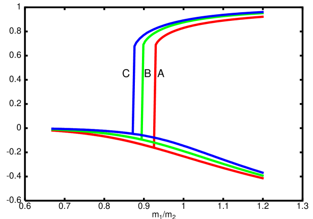
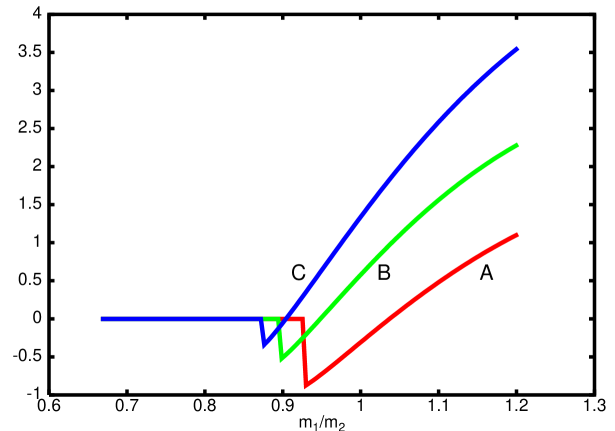
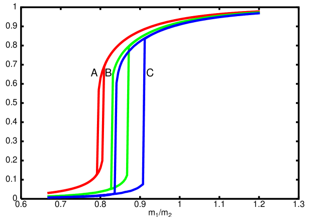
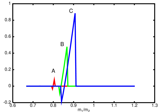
(a) (b) (c) (d)

Figure 5: These figures show the results of a typical set of experiments of a specific line in the parameter space, with the results projected on the $\frac{m_{1}}{m_{2}}$-axis. Figures (a) and (b) correspond to a lattice of type (a), while figures (c) and (d) correspond to a lattice of type (b). In the figures (a) and (c) the value of $\frac{\phi_{1}(0,0)}{\sqrt{6}f}$ is plotted, while in the figures (b) and (d) the relative energy differences of the two branches of the hysteresis plotted in pro-mils. The lines A, B and C correspond to 25$\times$25 (27$\times$27), 50$\times$50 (54$\times$54) and 100$\times$100 (108$\times$108) lattice points respectively describing the core structure.

Now let us examine and compare the figures 5(b) and 5(d). First we note that the relative energy differences are very small, being of the order of pro-mils. This is one of the reasons why the minimal relative energy difference step in the cooling mechanism is chosen so small, of the order of $10^{-5}$ pro-mil. In the regions where both branches of the hysteresis give the same configuration, see figures 5(a) and 5(c), the relative energy difference is equal to zero on the scale of the figures 5(b) and 5(d). The other segment of the curves is the interesting part, in figure 5(b) and 5(d). The point where this segment of the curves goes to zero is the point where the spherically magnetic monopole solution is no longer the lowest energy configuration within our ansatz, i.e., it is the point where the monopole becomes globally unstable. As we use more lattice points to probe this meta-stability this point moves only very slightly. Typically one should extrapolate the results to infinitely many points, but here we can use a different approach. We will exploit the results of the two different types of lattice. In the limit of infinitely many lattice points both lattice types will move to the same point. However in the figure 5(b) we see that this point in approached from the right while in figure 5(d) it is approached from the left when increasing the number of lattice points. Obviously this helps us to determine the position of the point where the monopole becomes globally unstable, as well as the error in the position of the point. So we may turn the lattice dependence into a useful tool to determine the global stability of the spherically symmetric monopole solution.

For most trajectories through the parameter space the same feature can be used to determine the point where the alice ring configuration becomes locally unstable with respect to the monopole. However this point is not as interesting, since the alice ring configuration is not necessarily an exact solution to the equations of motion. Both lattice types also show a local instability of the spherically symmetric monopole solution. In figure 5(c) this happens at a clear point, but from figure 5(a) where the monopole changes into a splitcore configuration, it is a bit harder to fix the point where this happens as it appears to be a continuous process. Although the position of this point is unclear, from figure 5(a), it is at least clear that this point moves in the same direction for both types of lattices as follows from figures 5(a) and 5(c).

With the help of the results of both types of lattice we determine the global instability point of the spherically symmetric monopole solution and local instability point of alice ring configuration. To determine the monopole instability point we only use the results from the lattices of type (b) as they clearly show the point where the monopole solution becomes locally unstable.

5 The meta-/instability results

Let us now turn to results of our investigations. First we describe how we extracted the results from the hysteresis type of experiments. There are two important results. In the first place, there is the line bounding the region in parameter space where the spherically symmetric magnetic monopole solution is no longer the lowest energy configuration. Crossing that line the solution only becomes meta-stable. Although our variational method does not prove that the configuration which has the lowest energy is a cheshire charged alice ring solution, in that case it actually does imply it, as we find that a cheshire charged alice ring configuration exists for those parameter values. In the second place there is the other line bounding the region where the spherically symmetric magnetic monopole solution is no longer a locally stable solution. Finally we also determined the line at which the alice ring configuration becomes locally unstable, but as explained before, this line is of least interest as the alice ring configuration (with our ansatz) is typically not a solution to the equations of motion of the model.

In figure 6(a-c) we give the results for the meta-stability and instability lines. Figure 6(c) shows the meta-stability line for the spherically symmetric magnetic monopole solution. As we showed in section 4.3 we can use both lattice types to determine the monopole meta-stability line as both lattice types move to this line from a different side as the number of lattice points increase. We determined the monopole meta-stability line up to the distance between the two monopole meta-stability lines determined from the data of both lattice types at the maximal number of lattice points we used. The plot shows the lines on which we did the hysteresis type of experiments, the two monopole meta-stability lines determined by the different lattice types and a shaded region which is to represent the error in the position of the monopole meta-stability line. Thus we did not extrapolate the results from both types of lattices to an infinite number of lattice points we just used the results from the lattices with the most lattice points to corner the meta-stability line, see figure 6(c). This line shows that the spherically symmetric magnetic monopole is not always the lowest energy solution and cuts the parameter space into two regions.

To determine the position of the instability line of the spherically magnetic monopole solution, see figure 6(b), we just use the results from the type (b) lattices as these show a clear point where the monopole becomes unstable. This does mean we have to extrapolate our results to a lattice with an infinite number of points. For all lines in the parameter space we investigated we observed that the change of the position, projected on the $\frac{m_{1}}{m_{2}}$-axis, of this point from the 27$\times$27 to the 54$\times$54 lattice is about twice as big as the change in the position from the 54$\times$54 to the 108$\times$108 lattice. We estimate the position of the monopole instability point by extrapolating this behavior to a lattice of an infinite number of lattice points. This means that the estimated position of the instability point lies at the same distance from the 108$\times$108-point as the 54$\times$54-point only on the other side. The error we estimate as twice this distance. In figure 6(b) we plotted these results. We plotted the lines on which we did the hysteresis experiments. The shaded region is to represent the error in the position of the monopole instability line and we plotted the instability line obtained from the data of the 108$\times$108 lattices. The estimate of the instability line itself is not plotted but is right in the middle of the shaded region.

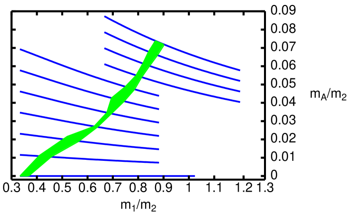
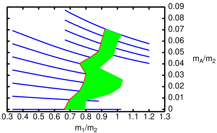
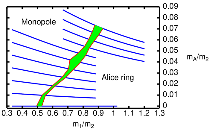
(a) (b) (c)

Figure 6: These figures show the stability results from the hysteresis type of experiments we did on the specific lines in the parameter space of the model. The shaded regions give the errors of the lines. Figure (a) shows the local instability line of the alice ring configuration. Figure (b) shows the monopole instability line and figure (c) shows the monopole meta-stability line.

In figure 6(a) we plotted the instability line of the alice ring configuration. For most of the lines through the parameter space we used the same technique as for the monopole meta-stability line, for the rest we used the same principle as we used for the monopole instability line.

Again we note that due to the fact that we used a variational approach the monopole meta-stability and instability lines are upper bounds in the sense that if less restrictions are forced upon the configurations these lines can only move to the left, i.e., in favor of the cheshire charged alice ring.

It is quite easy to understand why the alice ring is the lowest energy configuration in the limit of large values of $\frac{m_{1}}{m_{2}}$ and the monopole is the lowest energy solution in the limit of small $\frac{m_{1}}{m_{2}}$. The two masses $m_{1}$ and $m_{2}$ correspond to energy costs in deviations of the Higgs field from the vacuum manifold. Deviations pure in the ’length’ of the Higgs field correspond to $m_{1}$. While deviations in the non-uniaxial direction correspond to $m_{2}$. In the limit of $\frac{m_{1}}{m_{2}}\to 0$ the non-uniaxial deviations are suppressed and the spherically symmetric (uniaxial) magnetic monopole is the lowest energy solution. In the limit of $\frac{m_{1}}{m_{2}}\to\infty$ one would expect an ’escape’ in the non-uniaxial direction. This signals the meta-stability of the monopole and implies that the cheshire charged alice ring is the lowest energy solution. In this case the length of the Higgs field never becomes zero as can bee seen in figure 4(b), i.e., the quantity $\left(1-\frac{Tr\Phi^{2}}{6f^{2}}\right)$ never becomes equal to one.

We pointed out that one of the main factors determining the monopole core meta-stability is the mass ratio $\frac{m_{1}}{m_{2}}$ of the charged and neutral Higgs particles. As the mass of the charged excitation becomes much smaller than the mass of the neutral excitation the ’t Hooft Polyakov magnetic monopole is expected to become meta-stable. Clearly this argument holds generically and one expects a core meta-/instability to be a general feature of the ’t Hooft Polyakov magnetic monopole in models with charged Higgs excitations. The nice thing of alice type models is that they naturally suggest an alternative configuration to the ’t Hooft Polyakov type monopoles: the magnetically cheshire charged alice loop.

6 Conclusions and outlook

In this paper we investigated the core structure of the unit charge magnetic monopole and discussed the numerical methods we employed in some detail. We already showed in a previous letter [3] that the core structure of the magnetic monopole is not necessarily spherically symmetric. The model has three mass scales, two of them refer to the Higgs field, one to its length and the other to deviation from the uniaxial direction. The third mass scale is set by the mass of the broken gauge fields. The topologically non-trivial boundary conditions can be met by an “escape” in a non-uniaxial direction. This possibility allows for the length of the Higgs field to stay finite in the core and not go to zero as would be necessary otherwise. As the ratio of the masses, $\frac{m_{1}}{m_{2}}$, increases it becomes harder energetically to decrease the length of the Higgs field and one would expect an escape in the non-uniaxial direction.

At the end of section 5 we argued that a core instability of the ‘t Hooft Polyakov magnetic monopole is a general feature of models with charged excitations of the Higgs field. The instability occurs in the region of the parameter space where the charged excitations are much lighter than the neutral excitations. In alice electrodynamics there is also an other, somewhat independent motivation to question the core stability of the spherically symmetric magnetic monopole, provided by the possibility of an alice ring which can carry a magnetic cheshire charge.

Within our ansatz we determined the meta- and instability regions of the spherically symmetric magnetic monopole. We also found that, as expected, the competing configuration is the magnetically cheshire charged alice ring. We did also stumble upon the somewhat unwanted splitcore configurations but fortunately they never became the lowest energy solutions. As we used a variational approach we cannot claim that the alice ring configurations we found are exact solutions to the equations of motion. However they do have every feature which one would expect from an exact alice ring solution. Also, because we used a variational approach the regions of meta-stability and global-stability of the spherically magnetic monopole are with respect to energetic upper bounds so that with respect to the exact solutions, these regions can only become smaller.

As a final comment we want to come back to the fact that the minimum value of $\frac{m_{1}}{m_{2}}=\frac{1}{3}$ for which the broken vacuum is the true vacuum. In section 5 we gave a simple explanation of why the spherically magnetic monopole becomes globally unstable in the limit of large values of $\frac{m_{1}}{m_{2}}$. In the opposite limit one would expect the monopole to be the spherically magnetic monopole to be the global stable solution. However as the minimum value of $\frac{m_{1}}{m_{2}}=\frac{1}{3}$ there is no guarantee that this ever happens. It could just be that in this or similar models the ‘t Hooft Polyakov type magnetic monopole is never globally stable.

Acknowledgment: This work was partially supported by the ESF COSLAB program.

References

- [1] G. ’t Hooft. Magnetic monopoles in unified gauge theories. Nucl. Phys., B79:276–284, 1974.
- [2] A. M. Polyakov. Particle spectrum in quantum field theory. JETP Lett., 20:194–195, 1974.
- [3] F. A. Bais and J. Striet. On a core instability of ’t Hooft Polyakov type monopoles. Phys. Lett., B540:319–323, 2002.
- [4] F. Alexander Bais and Per John. Core deformations of topological defects. Int. J. Mod. Phys., A10:3241–3258, 1995.
- [5] A. S. Schwarz. Field theories with no local conservation of the electric charge. Nucl. Phys., B 208:141, 1982.
- [6] Mark Alford, Katherine Benson, Sidney Coleman, John March-Russell, and Frank Wilczek. Zero modes of nonabelian vortices. Nucl. Phys., B 349:414–438, 1991.
- [7] R. Shankar. More monopoles. Phys. Rev., D 14:1107, 1976.
- [8] J. Striet and F. A. Bais. Simple models with Alice fluxes. Phys. Lett., B497:172–180, 2000.
- [9] Howard Georgi and Sheldon L. Glashow. Spontaneously broken gauge symmetry and elementary particle masses. Phys. Rev., D 6:2977–2982, 1972.
- [10] Jr. E.C.Gartland and S.Mkaddem. Instability of radial hedgehog configurations in nematic liquid crystals under Landau-de Gennes free energy models. Phys. Rev. E, 59:563–567, 1999.
- [11] S.Mkaddem and Jr. E.C.Gartland. Fine struture of defects in radial nematic droplets. Phys. Rev. E, 62:6694–6705, 2000.