Observational Constraints on Cosmic String Production During Brane Inflation

Abstract

Overall, brane inflation is compatible with the recent analysis of the WMAP data. Here we explore the constraints of WMAP and 2dFGRS data on the various brane inflationary scenarios. Brane inflation naturally ends with the production of cosmic strings, which may provide a way to distinguish these models observationally. We argue that currently available data cannot exclude a non-negligible contribution from cosmic strings definitively. We perform a partial statistical analysis of mixed models that include a sub-dominant contribution from cosmic strings. Although the data favor models without cosmic strings, we conclude that they cannot definitively rule out a cosmic-string-induced contribution of $\sim 10\%$ to the observed temperature, polarization and galaxy density fluctuations. These results imply that $G\mu\lesssim 3.5\times 10^{-7}(\lambda/0.25)\sqrt{B/0.1}$, where $\lambda$ is a dimensionless parameter related to the interstring distance, and $B$ measures the importance of perturbations induced by cosmic strings. We argue that, conservatively, the data available currently still permit $B\lesssim 0.1$. Precision measurements sensitive to the B-mode polarization produced by vector density perturbation modes driven by the string network could provide evidence for these models. Accurate determinations of $n_{s}(k)$, the scalar fluctuation index, could also distinguish among various brane inflation models.

I Introduction

Observations of the cosmic microwave background (CMB) cobe ; new support the idea that the standard big bang phase of the expansion of the Universe was preceded by inflation guth . Recent results from the Wilkinson Microwave Anisotropy Probe (WMAP) wmap_bennett ; wmap_spergel ; wmap_verde ; wmap_peiris ; wmap_komatsu constrain the properties of proposed inflationary models tightly, but although some models are now excluded, numerous possibilities remain. A further challenge to observational cosmology is to try to hone in on a small class of viable models, even if identifying a single, correct theory of inflation may prove impracticable.

All of the data collected up until now are consistent with a relatively pristine Universe in which the perturbations observed today result from the amplification and distortion of a relatively featureless, Gaussian spectrum of fluctuations produced by quantum effects during inflation. However, it is likely that inflation itself could have left behind other remnants – such as cosmic strings – which could actively perturb both the CMB and dark matter of the Universe up to the present day.

It is well-known that cosmic strings cannot be wholly responsible for either the CMB temperature fluctuations or the observed clustering of galaxies aletal ; roughly speaking, the implied limits on the cosmic string tension $\mu$ allowed by observations is $G\mu\lesssim 10^{-6}$. However, now that cosmology has entered an era in which the properties of the Universe are being revealed to unprecedented precision, a natural question is to what extent the observations can allow previously unwanted ingredients, such as cosmic strings (e.g. bouchet ). Indeed, as the precision of cosmological observations increases, we might hope to be able to distinguish among numerous presently viable models for inflation by the properties of the cosmic strings they predict.

Although the idea that inflationary cosmology might lead to cosmic string formation is not new kofman , it has received new impetus from the brane world scenario suggested by superstring theory. In brane world cosmology, standard model particles and interactions correspond to open string (brane) modes, while the graviton, the dilaton and the radions are closed string (bulk) modes. Thus, our 3D Universe can be thought of as residing on a brane or stack of branes with three dimensions of cosmological size. These branes in turn reside in extra dimensions that are compactified. In such a model, inflation can result during the collisions of branes coalescing to form, ultimately, the brane on which we live dvali-tye .

In these brane inflation models, the separations between branes in the compactified dimensions are scalar fields (open string modes) that can act as inflatons, with the interaction potential between spatially separated branes providing the inflaton potential. Details of the brane inflation scenario depend on both qualitative and quantitative features, such as whether collisions involve a brane-antibrane pair burgess or two branes coalescing at an angle rabadan , as well as parameters such as the sizes of the compactified dimensions collection ; jst . Qualitatively, though, it appears easy to find models that predict adiabatic temperature and dark matter fluctuations capable of reproducing all currently available observations. A seemingly unavoidable outcome of brane inflation, though, is the production of a network of cosmic strings jst ; costring , whose effects on cosmological observables ranges from negligible to substantial, depending on the specific brane inflationary scenario jst2 .

Although cosmic string production towards the end of inflation is possible in field theory models kofman , the scaling properties of the cosmic string networks in brane inflationary scenarios are different than that in the familiar 3+1 D simulations, since intercommutation probabilities are smaller as a consequence of the existence of extra dimensions. In addition to placing constraints on the amplitude of string induced perturbations of the CMB, we show that the results place limits on $G\mu/\lambda$, where $\mu$ is the string tension and $\lambda\leq 1$ is related to the interstring distance as a fraction of the horizon. The value of $\lambda$ is sensitive to the intercommutation rate of strings, however the exact relation is expected to be model-dependent.

Here we shall first review the essential points of brane inflation, and examine the constraints imposed by the WMAP observations if we ignore the contribution from cosmic strings. These constraints allow us to delineate a range of possible cosmic string tensions. Then, we assess quantitatively the extent to which cosmic strings can contribute to the CMB temperature fluctuations and power spectra of dark matter density perturbations. In this analysis, we hold properties of the background cosmological model fixed to their best fit values, as determined by WMAP wmap_spergel without cosmic strings. (A more detailed analysis that varies the background cosmology as well is under way.) Although the available data favor models without cosmic strings, they may still allow, within the uncertainties, a contribution from string-induced perturbations of up to 10%. They also imply scalar perturbation indices $n_{s}(k)$ which, although still consistent with a broad range of models, may be able to discriminate among them in future. We also compute the dark matter density perturbation power spectrum, and compare with observational determinations from the 2dFGRS galaxy survey 2dF . We discuss the interpretation of these results in terms of the string tension and efficiency with which the cosmic string network decays via intercommutation of string segments, which is reduced in a Universe with extra dimensions. Finally, we discuss the prospects for detecting B-mode polarization, which is expected to be a prominent signature of a cosmic string network, in view of the constraints implied by our analysis.

II Brane Inflation and Cosmic String Properties

Recently, the brane world scenario suggested by superstring theory was proposed, where the standard model of the strong and electroweak interactions are open string (brane) modes while the graviton and the radions are closed string (bulk) modes. The relative brane positions (i.e., brane separation) in the compactified dimensions are scalar fields that have just the right properties to act as inflatons. Thus, the brane inflation scenario emerges naturally in the brane world dvali-tye . In this picture, the inflaton potential is due to the exchange of closed string modes between branes; this is the dual of the one-loop partition function of the open string spectrum, a property well-studied in string theory Polchinski1 . This interaction is of gravitational strength, resulting in a very weak (flat) potential, ideally tailored for inflation.

The potential is essentially dictated by the attractive gravitational (and the Ramond-Ramond) interaction between branes. As the branes move towards each other, slow-roll exponential inflation takes place. This yields an almost scale-invariant power spectrum for density perturbation, except there is a slight red-tilt (at a few percent level). As they reach a distance around the string scale, the inflaton potential becomes quite steep so that the slow-roll condition breaks down. At around the same time, a complex tachyon appears, so inflation ends rapidly as the tachyon rolls down its potential. In effect, inflation ends when the branes collide, heating the universe to start the standard big bang phase of cosmological expansion. This brane inflationary scenario may be realized in a number of ways collection ; jst . The scenario is simplest when the radion and the dilaton (bulk) modes are assumed to be stabilized by some unknown non-perturbative bulk dynamics at the onset of inflation. Since the inflaton is a brane mode, and the inflaton potential is dictated by the brane mode spectrum, it is reasonable to assume that the inflaton potential is insensitive to the details of the bulk dynamics.

Coupling of the tachyon to inflaton and standard model fields can allow efficient heating of the universe if certain conditions on the coupling of the tachyon to standard model particles are met stw . As the tachyon rolls down its potential, besides heating the universe, the vacuum energy also goes to the production of defects, in particular, cosmic strings. The effect of the resulting cosmic string network may be negligible or rather substantial, depending on the particular brane inflationary scenario jst2 . However, in all cases, we expect the density perturbation power spectrum in CMB to be dominated by the adiabatic fluctuations arising from quantum fluctuations of the inflaton during brane inflation, not by the nonadiabatic contributions from cosmic strings. However, the contribution to the density perturbation power spectrum in CMB coming from the cosmic string network may be large enough to be observable.

We devote this section to a review of the implications of brane inflation. For a broad set of models, we present results for the slow roll evolution, fluctuation spectra, string mass scale, and associated cosmic string tension. (These results follow directly from the treatments in Refs. collection ; jst ; burgess ; costring ; jst2 .) We consider the collision of a ${\rm D}p$ brane with a ${\rm D}p$ brane at an angle $\theta$; collision with a ${\rm D}p$ antibrane corresponds to $\theta=\pi$. (Here and throughout this section, we follow jst , which contains more details and discussion). Of the ten spacetime dimensions, one is the time, three are the large spatial dimensions we live in, and the rest are compactified. Of the compact dimensions, $p-3$ are parallel to the brane, and we take their compactification lengths to be $\ell_{\parallel}=2\pi r_{\parallel}$, implying a volume $V_{\parallel}=\ell_{\parallel}^{p-3}$. Of the remaining $d=9-p$ dimensions, we take $d-d_{\perp}$ to be compactified with a size $2\pi/M_{s}$, where $M_{s}$ is the string scale, while the remaining $d_{\perp}$ are compactified with a size $\ell_{\perp}=2\pi r_{\perp}>2\pi/M_{s}$. The 10-dimensional gravitational coupling constant is

$$\kappa^{2}=8\pi G_{10}={g_{s}^{2}(2\pi)^{7}\over 2M_{s}^{8}}$$ (1)

where $g_{s}$ is the expectation value of the dilatonic string coupling, which is related to the standard model gauge coupling $\alpha(r_{\parallel})$ on a scale $1/r_{\parallel}$ by

$$g_{s}=2(M_{s}r_{\parallel})^{p-3}\alpha(r_{\parallel})~{};$$ (2)

the 4-dimensional Planck scale $M_{P}=(8\pi G)^{-1/2}$ is then

$$g_{s}^{2}M_{P}^{2}={M_{s}^{2}(M_{s}r_{\perp})^{d_{\perp}}(M_{s}r_{\parallel})^{p-3}\over\pi}~{}.$$ (3)

The outcome of brane inflation will therefore depend on several parameters, $p$, $d_{\perp}$, $r_{\perp}$, $r_{\parallel}$ and $\alpha(r_{\parallel})$.

We will distinguish between two different potentials for the interaction between branes, depending on their separations. (See burgess ; rabadan ; collection .) For some scenarios, a fixed lattice of branes is considered to be spread throughout the compactified dimensions, with a moving brane placed inside one lattice square. At separations small compared to the lattice size of the compactification topology, the interaction is “Coulombic”, with a potential of the form $V(y)=V_{0}-U/y^{d_{\perp}-2}$ for a separation $y$ in the large compact dimensions. This potential is suitable for inflation resulting from the collision of a pair of relatively nearby branes at a small angle rabadan . When the separation is nearly equal to the lattice size, an expansion about zero displacement from the anti-podal point gives $V(y)=V_{0}-U^{\prime}y^{\sigma}$, where $\sigma$ depends on the compactification topology. This potential is suitable for the brane-anti-brane scenario (which corresponds to branes at angle $\pi$). In the next two subsections, we summarize the inflation scenario for interbrane potentials of these two general forms.

II.1 Coulombic Inflation

Consider a potential of the form

$$V(\psi)=V_{0}\left(1-{\eta\over(d_{\perp}-2)\psi^{d_{\perp}-2}}\right)~{},$$ (4)

with $\psi\propto y$, the interbrane spacing; for the special case $d_{\perp}=2$ this becomes a logarithmic potential, but the results we derive below may be applied to this special case. (We only consider $d_{\perp}-2\geq 0$ here to simplify our analysis, since the results generalize easily to the logarithmic case.) In the slow roll approximation, the equation of motion for $\psi$ becomes

$${d\psi\over dL}=-{\eta M_{P}^{2}\over\psi^{d_{\perp}-1}},$$ (5)

where $L=\ln a$ is the logarithm of the scale factor $a(t)$, which we take to be zero at the start of inflation. The slow roll solution is then

$$\psi=\left[\psi_{i}^{d_{\perp}}-d_{\perp}\eta M_{P}^{2}L\right]^{{1\over d_{\perp}}}=\left[d_{\perp}\eta M_{P}^{2}(L_{\rm inf}-L)\right]^{1\over d_{\perp}}\equiv\left(d_{\perp}\eta M_{P}^{2}L_{r}\right)^{1\over d_{\perp}}~{},$$ (6)

where the starting value of the field is $\psi_{i}$, the total number of e-folds in inflation, is

$$L_{\rm inf}={\psi_{i}^{d_{\perp}}\over d_{\perp}\eta M_{P}^{2}}~{},$$ (7)

and $L_{r}=L_{\rm inf}-L$ is the total number of e-folds remaining in inflation. The curvature fluctuation spectrum is then

$$\Delta^{2}_{\cal R}(k)={H^{4}\over 4\pi^{2}\dot{\psi}^{2}}={V_{0}(d_{\perp}L_{r})^{2\left(1-{1\over d_{\perp}}\right)}\over 12\pi^{2}\eta^{{2\over d_{\perp}}}M_{P}^{2+{4\over d_{\perp}}}}$$ (8)

where $L_{r}$ is evaluated when $k/a=H$, or $\ln(k/k_{0})=L_{r,0}-L_{r}$, where $k_{0}$ is a reference scale, which crosses with $L_{r,0}$ e-folds remaining in inflation. The fluctuation spectrum is very flat, with only slowly varying scalar index, $n_{s}(k)$:

$$n_{s}(k)-1 = {d\ln\Delta^{2}_{\cal R}(k)\over d\ln k}=-{2\over L_{r}(k)}\left(1-{1\over d_{\perp}}\right)\simeq-0.03\left[{60\over L_{r}(k)}\right]\left(1-{1\over d_{\perp}}\right)$$

$${dn_{s}(k)\over d\ln k} = -{2\over L_{r}^{2}(k)}\left(1-{1\over d_{\perp}}\right)\simeq-6\times 10^{-4}\left[{60\over L_{r}(k)}\right]^{2}\left(1-{1\over d_{\perp}}\right)~{},$$ (9)

both of which are in the range of uncertainty of the determinations in wmap_spergel .

The challenge to this, or any other, inflation model is to have sufficient inflation as well as small curvature fluctuation. Since the precise value of $L_{\rm inf}$ depends on initial conditions as well as parameters of the model, let us first consider the constraints on the latter implied by comparing Eq. (8) to the WMAP result $\Delta^{2}_{\cal R}(k_{0})=2.95\times 10^{-9}A(k_{0})$ with $A(k_{0})=0.9\pm 0.1$. To do this, let us consider a particular model with $p=4$ and a small collision angle, $\theta$; then we have

$$\psi = y\sqrt{\tau_{4}\ell_{\parallel}\over 2}$$

$$V_{0} = {\tau_{4}\ell_{\parallel}\theta^{2}\over 4}$$

$${\tau_{4}\ell_{\parallel}\over 2} = {M_{s}^{4}\over 32\pi^{3}\alpha(r_{\parallel})}$$

$$\eta = {\beta(d_{\perp})\over 16\pi}~{}\theta~{}M_{s}^{6-d_{\perp}}~{}\left({\tau_{4}\ell_{\parallel}\over 2}\right)^{d_{\perp}-4\over 2}$$

$$\Delta^{2}_{\cal R}(k) = {\left(\theta d_{\perp}L_{r}\right)^{2\left(1-{1\over d_{\perp}}\right)}\over 24\left[64\beta(d_{\perp})\right]^{2\over d_{\perp}}\pi^{2+{10\over d_{\perp}}}[\alpha(r_{\parallel})]^{4\over d_{\perp}}}~{}\left({M_{s}\over M_{P}}\right)^{2+{4\over d_{\perp}}}~{},$$ (10)

where

$$\tau_{p} = \frac{M_{s}^{p+1}}{(2\pi)^{p}g_{s}}$$ (11)

$$\beta = \left\{\begin{array}[]{cc}{{1\over{2\pi^{d_{\perp}/2}}}{\Gamma\left({d_{\perp}-2}\over 2\right)}}&d_{\perp}>2\\ {1\over{\pi}}&d_{\perp}=2.\end{array}\right.$$ (14)

Let us consider the specific example $d_{\perp}=2$; for this case we find

$$\Delta^{2}_{\cal R}(k)={\theta L_{r}\over 768\pi^{6}[\alpha(r_{\parallel})]^{2}}\left({M_{s}\over M_{P}}\right)^{4}\quad\qquad\qquad[d_{\perp}=2]~{},$$ (15)

and therefore the string scale is determined to be

$${M_{s}\over M_{P}}\simeq 2.5\times 10^{-2}[25\alpha(r_{\parallel})]^{1/2}[A(k_{0})]^{1/4}\left({10\over\theta L_{r}}\right)^{1/4}\qquad[d_{\perp}=2]$$ (16)

that is, on the same order of energy as the GUT scale, $10^{15}$ GeV. Larger $d_{\perp}$ leads to smaller $M_{s}/M_{P}$; thus if $d_{\perp}=4$ we find

$$\Delta^{2}_{\cal R}(k)={(\theta L_{r})^{3/2}\over 12\sqrt{2}\pi^{7/2}\alpha(r_{\parallel})}\left({M_{s}\over M_{P}}\right)^{3}\quad\qquad\qquad[d_{\perp}=4]~{},$$ (17)

which in turn requires

$${M_{s}\over M_{P}}\simeq 1.6\times 10^{-3}[25\alpha(r_{\parallel})]^{1/3}[A(k_{0})]^{1/3}\left({10\over\theta L_{r}}\right)^{1/2}\qquad[d_{\perp}=4]~{}.$$ (18)

The total number of e-folds in inflation is

$$L_{\rm inf} = {(M_{s}y_{i})^{d_{\perp}}M_{s}^{2}\over 64\pi^{5}\beta(d_{\perp})\theta[\alpha(r_{\parallel})]^{2}M_{P}^{2}}={\pi^{d_{\perp}(d_{\perp}-1)\over d_{\perp}+2}(2\zeta_{i}M_{s}r_{\perp})^{d_{\perp}}\over\theta^{3d_{\perp}\over d_{\perp}+2}(d_{\perp}L_{r})^{2(d_{\perp}-1)\over d_{\perp}+2}}\left[{3\Delta^{2}_{\cal R}(k)\over 8\beta(d_{\perp})\alpha^{2}(r_{\parallel})}\right]^{d_{\perp}\over d_{\perp}+2}$$ (19)

$$\simeq {0.025[A(k_{0})]^{1/2}\over[25\alpha(r_{\parallel})](10\theta)}\left({10\over\theta L_{r}}\right)^{1/2}(\zeta_{i}M_{s}r_{\perp})^{2}\qquad[d_{\perp}=2]$$

$$\simeq {0.025[A(k_{0})]^{2/3}\over[25\alpha(r_{\parallel})]^{4/3}(10\theta)}\left({10\over\theta L_{r}}\right)(\zeta_{i}M_{s}r_{\perp})^{4}\qquad[d_{\perp}=4]~{},$$

where we have let $y_{i}=2\pi r_{\perp}\zeta_{i}$ with $\zeta_{i}\lesssim 1$. To get $L_{\rm inf}\gtrsim 60$, we must require $\zeta_{i}M_{s}r_{\perp}\gtrsim 50$ for $d_{\perp}=2$ or $\zeta_{i}M_{s}r_{\perp}\gtrsim 10$ for $d_{\perp}=4$. Note, though, that for large $\theta$, it is not possible to have enough expansion during inflation. In this case, the images of one brane exert non-trivial forces on the other brane, resulting in a power-law type potential.

II.2 Power Law Inflation

Next, we consider potentials of the form

$$V(\psi)=V_{0}\left(1-\eta\psi^{\sigma}\right)~{};$$ (20)

such potentials arise for a brane situated near the origin. The value of $\sigma$ depends on the compactification topology. For hypercubic compactification, $\sigma=4$, whereas in other cases, $\sigma=2$. Note that in actuality the potential need not depend just on interbrane separation in such a picture, and the trajectory of the brane can be complicated. Here, though, we confine ourselves to simple one dimensional (diagonal) brane motion.

Following Eq. (20), we see that the origin – $\psi=0$ – is an unstable equilibrium point, and any perturbation away from it will result in slow motion of the brane. For $\sigma>2$, the slow roll solution is

$$\psi=[\psi_{i}^{\sigma-2}-\sigma(\sigma-2)\eta M_{P}^{2}L]^{1\over\sigma-2}=[\sigma(\sigma-2)\eta M_{P}^{2}L_{r}]^{1\over\sigma-2}~{},$$ (21)

and the total number of e-folds in inflation is

$$L_{\rm inf}={\psi_{i}^{\sigma-2}\over\sigma(\sigma-2)\eta M_{P}^{2}},$$ (22)

where $\psi_{i}$ is the starting value for the inflaton. Quantum fluctuations will imply $\psi_{i}=\zeta_{i}H/2\pi$, where $\zeta_{1}\sim 1$. The curvature fluctuation spectrum is

$$\Delta^{2}_{\cal R}(k)={V_{0}(\sigma-2)^{2}[\sigma(\sigma-2)\eta]^{2\over\sigma-2}M_{P}^{2(4-\sigma)\over\sigma-2}L_{r}^{2(\sigma-1)\over\sigma-2)}\over 12\pi^{2}}~{}.$$ (23)

The implied fluctuation spectrum is acceptably flat:

$$n_{s}(k)-1={d\ln\Delta^{2}_{\cal R}(k)\over d\ln k} = -{2(\sigma-1)\over(\sigma-2)L_{r}(k)}\simeq-{0.03(\sigma-1)\over\sigma-2}\left[{60\over L_{r}(k)}\right]$$

$${dn_{s}(k)\over d\ln k} = -{2(\sigma-1)\over L_{r}^{2}(k)(\sigma-2)}\simeq-6\times 10^{-4}\left({\sigma-1\over\sigma-2}\right)\left[{60\over L_{r}(k)}\right]^{2}~{}.$$ (24)

For $\sigma=4$, Eqs. (23) and (22) become

$$\Delta^{2}_{\cal R}(k) = {8\eta V_{0}L_{r}^{3/2}\over 3\pi^{2}}$$

$$L_{\rm inf} = {\zeta_{i}^{2}V_{0}\over 96\pi^{2}M_{P}^{4}(\eta V_{0})}~{};$$ (25)

the observational constraints on the curvature fluctuation spectrum therefore require

$$\eta V_{0}={3\pi^{2}\Delta^{2}_{\cal R}(k)\over 8L_{r}^{3/2}}\simeq 2.5\times 10^{-11}A(k_{0})\left({60\over L_{r}}\right)^{3/2}~{},$$ (26)

i.e. the potential must be extremely flat. This requirement is well-known from studies of new inflation, which sometimes idealize the potential to Eq. (20) with a small dimensionless parameter $\lambda$ equivalent to $\eta V_{0}$. In Ref. jst , a particular toroidal compactification is proposed where this small parameter is ($F$ is a geometrical factor related to the compactification geometry)

$$\eta V_{0}\simeq{g_{s}\theta^{4}F\beta\over 16\pi\alpha^{3}}\left({M_{s}\over M_{P}}\right)^{4}~{},$$ (27)

which can be small enough for $\theta\sim 0.1$ provided that

$${M_{s}\over M_{P}}\simeq 10^{-3}~{}.$$ (28)

In this picture, the flatness of the effective potential is attributed to a relatively small value of the string scale compared with the Planck mass.

Special treatment is required for $\sigma=2$, which is expected for any non-hypercubic compactification topology. For this case, the scale factor grows like a powerlaw in time during slow roll:

$$\psi=\psi_{i}\left({a\over a_{i}}\right)^{2\eta M_{P}^{2}}=\psi_{f}\left({a\over a_{f}}\right)^{2\eta M_{P}^{2}}~{},$$ (29)

where $\psi_{f}$ and $a_{f}$ are the values of the field and scale factor at the end of slow rolling. Since $d\ln\psi/d\ln a=2\eta M_{P}^{2}$, we require $\eta M_{P}^{2}\ll 1$ for slow rolling. It is easy to see that for this potential, $\ddot{\psi}/3H\dot{\psi}=2\eta M_{P}^{2}/3\ll 1$. Slow roll ends, for this potential, only when $\dot{\psi}^{2}/2V_{0}=2\eta^{2}M_{P}^{2}\psi^{2}/3\simeq 1$, or $\psi_{f}\simeq(\eta M_{P})^{-1}\gg M_{P}$, or when the polynomial approximation to the potential fails, which happens when the brane moves a substantial fraction of a lattice spacings. The total number of e-folds in inflation is

$$L_{\rm inf}={\ln(\psi_{f}/\psi_{i})\over 2\eta M_{P}^{2}}={\ln(y_{f}/y_{i})\over 2\eta M_{P}^{2}}~{}.$$ (30)

The curvature fluctuation spectrum for this case is

$$\Delta^{2}_{\cal R}(k)={(H/2\pi\psi_{f})^{2}e^{4\eta M_{P}^{2}L_{r}}\over 4(\eta M_{P}^{2})^{2}}={(H/2\pi\psi_{i})^{2}(a_{i}/a)^{4\eta M_{P}^{2}}\over 4(\eta M_{P}^{2})^{2}}={(H/2\pi\psi_{i})^{2}(a_{i}H/k)^{4\eta M_{P}^{2}}\over 4(\eta M_{P}^{2})^{2}}~{},$$ (31)

where evaluating at horizon crossing implies that $k=Ha$, which has been used to get the final form of the spectrum. In this case,

$$n_{s}-1={d\ln\Delta^{2}_{\cal R}(k)\over d\ln k}=-4\eta M_{P}^{2}~{},$$ (32)

which is independent of $k$. The WMAP analysis implies that $\eta M_{P}^{2}\lesssim 0.01$. From the first form of Eq. (31), and $\eta M_{P}^{2}\simeq 0.01$, it follows that the observed temperature fluctuations can be accounted for if ($V_{0}=2\tau_{4}\ell_{\parallel}$)

$${H\over 2\pi\psi_{f}}\sim(2\pi M_{P}y_{f})^{-1}\sim 10^{-7}\left({\eta M_{P}^{2}\over 0.01}\right)~{},$$ (33)

in which case $L_{\rm inf}\sim 10^{3}$. For $y_{f}\simeq 2\pi r_{\perp}$, this relation implies

$${M_{s}\over M_{P}}\sim 10^{-6}\left({\eta M_{P}^{2}\over 0.01}\right)~{}M_{s}r_{\perp}~{},$$ (34)

which is generally smaller than our previous estimates unless $M_{s}r_{\perp}\sim 10^{3}$.

II.3 Cosmic String Properties

Because the inflaton and the ground state open string modes responsible for defect formation are different, and the ground state open string modes become tachyonic and develop vacuum expectation values only towards the end of the inflationary epoch, various types of defects (lower-dimensional branes) may be formed. A priori, defect production after inflation may be a serious problem. Fortunately, it is argued in Ref.jst ; costring that, from the properties of superstring/brane theory and the cosmological evolution of the universe, the only defects copiously produced are cosmic strings. In superstring theory, D$p$-branes come with either odd $p$ (in IIB theory) or even $p$ (in IIA theory). The collision of a D$p$-brane with another D$p$-brane at an angle (or with an anti- D$p$-brane) yields D$(p-2)$-solitons (i.e., codimension 2). Topologically, a variety of defects may be produced. Because they have even codimensions with respect to the branes that collide, they have specific properties Sen1 . Cosmologically, since the compactified dimensions tangent to the brane are smaller than the Hubble size, the Kibble mechanism works only if all the codimensions are tangent to the uncompactified dimensions. As a consequence, only cosmic strings may be copiously produced jst ; costring .

The observational imprint of cosmic strings is determined primarily by the product of Newton’s constant and the cosmic string tension, $G\mu$, assuming the evolution of the string network can reach the scaling regime. The value of $\mu$ implied by superstring cosmology depends on several parameters, but is most sensitive to the string scale, $M_{s}$. To get an order of magnitude estimate, we may use the small $\theta$ case, which is arguably the most likely inflationary scenario.

The cosmic strings may be D$1$-branes, but most likely, they are D$(p-2)$-branes wrapping around $(p-3)$-cycles in the compactified dimensions. If the D$1$-brane is the cosmic string (i.e., $p=3$), its tension is simply the cosmic string tension:

$$\mu=\tau_{1}={M_{s}^{2}\over 2\pi g_{s}}~{}.$$ (35)

However, we expect the string coupling generically to be $g_{s}{\ \lower-1.2pt\vbox{\hbox{\hbox to0.0pt{$>$\hss}\lower 5.0pt\vbox{\hbox{$\sim$}}}}\ }1$. (It is well-known that radion and dilaton moduli are not stabilized by perturbative dynamics in string theory. Presumably, any superstrongly coupled string model is dual to a weakly coupled one, and thus cannot stabilize the moduli either. We therefore expect a moderately strong string coupling, since only in this case will we find non-trivial dynamics.) To obtain a theory with a weakly coupled sector in the low energy effective field theory (i.e., the standard model of strong and electroweak interactions with weak gauge coupling constant $\alpha$), it then seems necessary to have the brane world picture, in which we have the D$p$-branes for $p>3$, where the $(p-3)$ dimensions are compactified to volume $V_{\parallel}$. Now the cosmic strings are D$(p-2)$-branes, with the $(p-3)$ dimensions compactified to the same volume $V_{\parallel}$. Noting that a D$p$-brane has tension $\tau_{p}=M_{s}^{p+1}/(2\pi)^{p}g_{s}$, the tension of such cosmic strings is

$$\mu=\frac{M_{s}^{p-1}V_{\parallel}}{(2\pi)^{p-2}g_{s}}=\frac{M_{s}^{2}v_{\parallel}}{2\pi g_{s}}=\frac{M_{s}^{2}}{4\alpha\pi}\simeq 2M_{s}^{2}$$ (36)

for $\alpha\simeq\alpha_{GUT}\simeq 1/25$. For one pair of branes at angle $\theta$, only this type of cosmic strings is produced topologically. For a large enough stack of branes colliding, the D$1$-branes may also be allowed topologically, but they are not produced cosmologically. Thus, $\mu\simeq 2M_{s}^{2}$ is a reasonably general estimate. We considered estimates of $M_{s}$ implied in various scenarios for brane inflation in § II.1 and II.2. These estimates are broadly consistent with

$$10^{-6}\gtrsim G\mu\gtrsim 10^{-11}~{},$$ (37)

although a smaller range is obtained in any specific model or class of setups. For example, for branes colliding at a small angle, a likely range is

$$5\times 10^{-7}\gtrsim G\mu\gtrsim 7\times 10^{-8}~{}.$$ (38)

Thus, brane inflation can lead to cosmic string tensions below, but not far below, current observational bounds.

II.4 Tensor modes

During slow roll, the tensor power is

$$\Delta_{h}^{2}(k)={128G^{2}V_{0}\over 3}={2V_{0}\over 3\pi^{2}M_{P}^{4}}$$ (39)

and is smaller than the scalar power by the factor

$$r(k)=8M_{P}^{2}\left({V^{\prime}\over V}\right)^{2}={8\over M_{P}^{2}}\left({d\phi\over d\ln a}\right)^{2}~{}.$$ (40)

How small $r(k)$ is depends on the specific brane inflation model. For branes intersecting at an angle $\theta$ we find that

$$\Delta_{h}^{2}(k) = {2V_{0}\over 3\pi^{2}M_{P}^{4}}={\theta^{2}M_{s}^{4}\over 96\pi^{5}\alpha(r_{\parallel})M_{P}^{4}}$$ (41)

$$= 3.3\times 10^{-12}~{}(10\theta)^{2}~{}[25\alpha(r_{\parallel})]\left[{10A(k_{0})\over\theta L_{r}}\right]\qquad\qquad\quad[d_{\perp}=2]$$

$$= 5.4\times 10^{-17}(10\theta)^{2}[25\alpha(r_{\parallel})]^{1/3}[A(k_{0})]^{4/3}\left({10\over\theta L_{r}}\right)^{2}\qquad\quad[d_{\perp}=4]~{}.$$

In this case, the amplitude of the scalar mode is smaller than the amplitude of the perturbations due to cosmic strings by a small numerical factor times $\theta^{2}$, unless cosmic string intercommutation is extremely inefficient; see § II.3 and III below. For powerlaw brane-antibrane inflation, $\theta\to\pi$, and $V_{0}=M_{s}^{4}/(2\pi)^{3}\alpha$ burgess ; jst , so for this case we find

$$\Delta_{h}^{2}(k)={M_{s}^{4}\over 12\pi^{5}\alpha M_{P}^{4}}~{}.$$ (42)

Nominally, these perturbations can be comparable to those induced by cosmic strings, although they may be relatively suppressed by the small numerical factor $(12\pi^{5}\alpha)^{-1}\simeq 0.007/(25\alpha)$. However, the spectrum of fluctuations produced by cosmic strings will still distinguish them from those due to primordial tensor modes. Both strings and the primordial tensor modes result in the B-type polarization of the CMBR. The predicted angular power spectrum, $C_{l}^{BB}$, has been calculated for tensor modes from inflation (see e .g. alessandro ). It has a generic feature that most of the power is on larger angular scales, in the region $l\lesssim 100$. This is very different from the shape of the $C_{l}^{BB}$ spectrum predicted by cosmic strings. There the dominant contribution comes from the vector modes and, as one can see from Fig. 4, most of the power is on smaller scales: $700\lesssim l\lesssim 1000$.

As of today, the B-type polarization has not been detected kovac and the experimental constraint on $r(k)$ is rather mild: $r(k_{0}=0.002{\rm Mpc}^{-1})\lesssim 0.71$ wmap_peiris .

III CMB, Matter Density and Polarization Power Spectra: Calculation and Interpretation

The fluctuations expected to arise from brane inflation should be an incoherent superposition of contributions from adiabatic perturbations initiated by curvature fluctuations $\Delta^{2}_{\cal R}(k)$ and active perturbations induced by the decaying cosmic string network. For example, the resulting CMB temperature maps will yield

$$C_{l}=WC_{l}^{\rm adiabatic}+BC_{l}^{\rm strings},$$ (43)

were $W$ and $B$ are weighting factors. Analogous expressions hold for matter density and polarization power spectra. In Eq. (43), the weight factors $W$ and $B$ determine the relative importance of the adiabatic and cosmic string contributions. We choose the weight factor $W$ so that $W=1$ when there are no cosmic strings.

In computing the combined effects of adiabatic and cosmic string perturbations, we have kept the cosmological background parameters fixed at their best-fit values according to wmap_spergel . In addition to $B$ and $W$, we vary the spectral index of the scalar curvature fluctuations, $n_{s}$. The tensor contribution to the adiabatic component was set to zero, since, as discussed in § II.4, it is likely to be small. When fitting to both WMAP and the 2dFGRS data, we considered two cases (described in more detail in § III.2): with bias $b$ fixed, and with $b$ being an additional parameter of the fit.

III.1 Cosmic strings and the CMBR

Perturbations due to cosmic strings were calculated using the model first introduced in aletal and further developed in levon ; gangui . The main idea is to represent the cosmic string network by a collection of uncorrelated, straight string segments moving with random, uncorrelated velocities. All segments are produced at some early epoch and, at every subsequent epoch, a certain fraction of the number of segments decays in a way that maintains network scaling. The length of each segment at any time is taken to be equal to the correlation length of the network which, together with the root mean square velocity of segments, are computed from the velocity-dependent one-scale model of Martins and Shellard MS96 . The positions of segments are drawn from a uniform distribution in space and their orientations are chosen from a uniform distribution on a two-sphere.

This model is a rather crude approximation of a realistic string network. However, with a suitable choice of model parameters, its main predictions for CMB and matter power spectra have been shown to be in agreement with results obtained using other local string sources joao ; copmagst . The main advantage of our model is its flexibility. For example, parameters can be chosen to describe stings with different scaling properties, different amounts of small scale structure etc. This is especially valuable when describing strings produced in brane inflation, since strings are expected to intercommute with a lower probability in the presence of extra spatial dimensions jst2 .

It is well known that properties and possible observational signatures of global and local strings can be dramatically different. Global strings predict almost no power on small angular scales for CMB temperature anisotropy pen_ps , while local strings produce a quite significant broad peak at $l\sim 450$ in a spatially flat universe aletal ; levon ; joao ; copmagst ; closed . Also, local strings develop a signification amount of small-scale structure over the course of their evolution, which tends to suppress the vector component of metric perturbations. For that reason one would expect the strength of the $B$-type polarization pen_pol sourced by global strings to be somewhat larger than that of local strings newwork .

Numerical simulations BenBouch ; AllenShellard90 ; AlTur89 show that during the radiation and matter dominated eras the string network evolves according to a scaling solution, which on sufficiently large scales can be described by two length scales. The first scale, $\xi(t)$, is the coherence length of strings, i. e. the distance beyond which directions along the string are uncorrelated. The second scale, $L(t)$, is the average inter-string separation. Scaling implies that both length scales grow in proportion to the horizon. Simulations indicate that $\xi(t)\sim t$, while $L(t)=\gamma t$, with $\gamma\approx 0.8$ in the matter era BenBouch ; AllenShellard90 . The one-scale model Vilenkin81b ; Kibble85 , in which the two length scales are assumed to be equal, has been quite successful in describing the general properties of cosmic string networks inferred from numerical simulations. These simulations have assumed that cosmic strings would reconnect on every intersection. It is of interest to us, however, to also consider the case when the reconnection probability is less than one. If strings can move and interact in extra dimensions then, while appearing to intersect in our three dimensions, they may actually miss each other. Hence, the effective intercommutation rate of these strings will generally be smaller than unity. As a consequence, one would expect more strings per horizon in these theories. Because of the straightening of wiggles on sub-horizon scales due to the expansion of the universe, one would still expect $\xi(t)\sim t$. However, the string density would increase, therefore reducing the inter-string distance. Hence, smaller inter-commutation probabilities imply smaller $\gamma$.

Consider a string network in a volume $V$ described by the two length scales introduced above. On average there is one string segment of length $\xi$ per volume $\xi L^{2}$. The rough number of such string segments is

$$N={V\over\xi L^{2}}\ .$$ (44)

If the energy per unit length is $\mu$, then the total energy of the string network is

$$E=N\mu\xi={V\mu\over L^{2}}\ .$$ (45)

and the energy density is just $\rho=E/V=\mu/L^{2}$.

Now suppose we want to calculate the effect of this string network on the CMB temperature anisotropy. In particular, we want to find the power spectrum, i. e. the 2-point function. For simplicity, let us assume that only $\rho(t)$ affects CMB (in general we would have to consider all components of the string network’s energy-momentum tensor $T_{\mu}^{\nu}$). Then to evaluate the CMB power spectrum it suffices to know the 2-point unequal time correlators $\langle\rho(k,t_{1})\rho(k,t_{2})\rangle$ at all $k$, $t_{1}$ and $t_{2}$. Here $\rho({\bf k},t)$ is the Fourier transform of $\rho({\bf x},t)$. The CMB power spectrum is roughly given by

$$C_{l}=\int dk\int dt_{1}\int dt_{2}\ \hat{L}_{l}(t_{1},t_{2},k)\big{[}\langle\rho(k,t_{1})\rho(k,t_{2})\rangle\big{]}\ ,$$ (46)

where $\hat{L}_{l}(t_{1},t_{2},k)$ is a linear operator.

Again, for simplicity, let us assume that $\xi(t)\sim t$ and $L=\gamma t$ at all times, namely that the network scales perfectly with time. We want to see how $C_{l}$, or equivalently $\langle\rho(k,t_{1})\rho(k,t_{2})\rangle$, depends on $\gamma$ and $\mu$. Let us also assume that the segments are straight.

At time $t$ there are roughly $N(t)=V/\xi L^{2}$ segments and

$$\rho(k,t)=\sum_{i=1}^{N(t)}\rho^{(i)}(k,t)\equiv\sum_{i=1}^{N(t)}\tilde{\rho}^{(i)}(k,t)\mu\xi(t)\ ,$$ (47)

where $\tilde{\rho}^{(i)}(k,t)=\rho^{(i)}(k,t)/(\mu\xi(t))$ to factor out dependences on $\mu$ and $\xi(t)$ (the phase of $\tilde{\rho}$ may still depend on $\xi(t)$ but the amplitude does not). Now we can write:

$$\langle\rho(k,t_{1})\rho(k,t_{2})\rangle=\sum_{i=1}^{N(t_{1})}\sum_{j=1}^{N(t_{2})}\langle\tilde{\rho}^{(i)}(k,t_{1})\rho^{(j)}(k,t_{2})\rangle\mu^{2}\xi(t_{1})\xi(t_{2}).$$ (48)

Because individual segments are statistically independent

$$\langle\tilde{\rho}^{(i)}(k,t_{1})\rho^{(j)}(k,t_{2})\rangle=\delta_{ij}\ \langle\tilde{\rho}^{(i)}(k,t_{1})\tilde{\rho}^{(i)}(k,t_{2})\rangle\ ,$$ (49)

and therefore

$$\langle\rho(k,t_{1})\rho(k,t_{2})\rangle=\sum_{i=1}^{{\rm min}[N(t_{1}),N(t_{2})]}\langle\tilde{\rho}^{(i)}(k,t_{1})\tilde{\rho}^{(i)}(k,t_{2})\rangle\mu^{2}\xi(t_{1})\xi(t_{2})$$ (50)

To interpret ${\rm min}[N(t_{1}),N(t_{2})]$ it might help to think that all segments were there at the initial time but over course of their evolution some of them decayed. For certainty, let us assume $t_{1}<t_{2}$ and therefore $N(t_{1})>N(t_{2})$. We can now write

$$\langle\rho(k,t_{1})\rho(k,t_{2})\rangle=\sum_{i=1}^{N(t_{2})}\langle\tilde{\rho}^{(i)}(k,t_{1})\tilde{\rho}^{(i)}(k,t_{2})\rangle\mu^{2}\xi(t_{1})\xi(t_{2})=N(t_{2})\langle\tilde{\rho}^{(1)}(k,t_{1})\tilde{\rho}^{(1)}(k,t_{2})\rangle\mu^{2}\xi(t_{1})\xi(t_{2})\ ,$$ (51)

where the last step is possible because all segments are statistically identical and hence

$$\langle\tilde{\rho}^{(i)}(k,t_{1})\tilde{\rho}^{(i)}(k,t_{2})\rangle=\langle\tilde{\rho}^{(1)}(k,t_{1})\tilde{\rho}^{(1)}(k,t_{2})\rangle\ \ \ {\rm for\ all}\ i.$$ (52)

Substituting $\xi\sim t$, $L=\gamma t$ and $N(t)=V/(\xi L^{2})\sim V/(\gamma^{2}t^{3})$ we find

$$\langle\rho(k,t_{1})\rho(k,t_{2})\rangle={V\over\gamma^{2}t_{2}^{3}}\mu^{2}t_{1}t_{2}\langle\tilde{\rho}^{(1)}(k,t_{1})\tilde{\rho}^{(1)}(k,t_{2})\rangle={\mu^{2}\over\gamma^{2}}\times F(k,t_{1},t_{2})\ ,$$ (53)

where $F(k,t_{1},t_{2})$ is independent of $\xi$ or $\mu$, and therefore

$$C_{l}^{\rm strings}\propto{\mu^{2}\over\gamma^{2}}\ .$$ (54)

Rather than working with the parameter $\gamma=L(t)/t$, we define a related parameter $\lambda\equiv l(\tau)/\tau$, where $l(\tau)$ is the comoving interstring distance, $L/a$, and $\tau$ is the conformal time, $d\tau=dt/a$. In our code we take parameter $\lambda$ to be a constant. Correspondingly, the meaning of the parameter $B$ is

$$B={C_{l}(\lambda,G\mu)\over C_{l}(\lambda_{0},G\mu_{0})}=\left[{\mu\lambda_{0}\over\mu_{0}\lambda}\right]^{2}$$ (55)

with $G\mu_{0}=1.1\times 10^{-6}$ and $\lambda_{0}=0.25$ adopted as reference values.

The relation between parameter $\lambda$ and the string intercommutation probability $p$ has been a subject of extensive research. Qualitative arguments in DV04 suggest that $\lambda\propto p^{1/2}$. However, these arguments do not take into account possible effects of small-scale structure on strings. Results of the most recent numerical simulations AS05 suggest that for $p>0.1$ the scaling string density is effectively the same as for $p=1$, while for smaller $p$ one should expect $\lambda\propto p^{0.3}$. Such weak dependence of $\lambda$ on $p$ can be explained by multiple opportunities for string reconnection during one crossing time, due to small-scale wiggles.

III.2 Methods

We have performed a partial statistical analysis in which we held the parameters of the background cosmological model (total, matter, baryon and dark energy density parameters, Hubble constant, reionization optical depth) fixed at their WMAP best fit values according to wmap_spergel . More specifically, we considered a flat $\Lambda$CDM universe with $\Omega_{\rm CDM}=0.225$, $\Omega_{b}=0.045$, $\Omega_{\Lambda}=0.73$, $H_{0}=71$ km/s/Mpc and $\tau=0.17$. The scalar spectral index $n_{s}$ was allowed to vary within bounds set by the prior $0.8\leq n_{s}\leq 1.2$, in increments of $\Delta n_{s}=1.25\times 10^{-3}$.

The string spectra were calculated only once, using the string model parameters chosen to produce spectra that roughly agree with aletal ; levon ; joao ; copmagst . In particular, we set $G\mu_{0}=1.1\times 10^{-6}$, which, if strings were the only source of inhomogeneity, would result in temperature anisotropy in a rough agreement with observations on COBE scales. The string intercommutation probability $\lambda$ was approximately $\lambda\sim 0.25$ and was allowed to vary only insignificantly during the radiation-matter domination transition.

The CMBR and linear matter power spectra for both adiabatic and string parts were computed using respectively modified versions of CMBFAST cmbfast . However, one cannot directly compare linear matter spectra outputted by CMBFAST to the galaxy clustering data published by the 2dFGRS team. We have “processed” the theoretical power spectrum $P^{th}(k)$ for both adiabatic and string components following a procedure similar to that prescribed in Section 5.1.4 of wmap_verde . First of all, we output $P^{th}(k)$ at the effective redshift of the 2dFGRS survey: $z_{\rm eff}=0.17$ (the valued suggested in wmap_verde ). Then we correct for the redshift space distortions using the approximate formula given in wmap_verde :

$$P^{th}(k)\rightarrow P^{th}_{z}(k)=(1+{2\over 3}\beta+{1\over 5}\beta^{2})P^{th}(k)\ ,$$ (56)

with $\beta=0.45$. We then convolve it with the 2dF window function 2dF using the matrix $M_{W}$ provided on the 2dFGRS website:

$$P^{th}_{z}(k)\rightarrow P_{W}(k)=\sum_{q}M_{W}(k,q)P^{th}_{z}(q)$$ (57)

and, finally, multiply by the bias factor to obtain the spectrum that can be compared to data:

$$P(k)=b^{2}P_{W}(k)$$ (58)

where $b=\Omega_{m}^{0.6}/\beta$.

We have chosen to fit to the binned version of WMAP data, for both temperature (TT) and cross temperature-polarization (TE) angular spectra. When fitting to WMAP+2dF we had a choice of making the bias $b$ an additional parameter or using a prescribed fixed value. We have investigated both possibilities and will refer to them the “$b$-free” and “$b$-fixed” model.

III.3 Results

We are interested in constraining the fractional contribution to the WMAP and 2dFGRS data given by Eq. (43). To do this properly, from first principles, would require using theoretical models with both cosmic strings and adiabatic perturbations to generate the relevant sky maps, and then compare these directly to the data to compute likelihood functions that can be used, along with appropriate priors, the posterior probability distributions for the parameters of the models. To get a quick and dirty bound on the most interesting parameter, $B$, we have chosen to adopt a simpler approach in which we treat the published results for $C_{l}$ of the TT and TE sky maps, and the 2dFGRS power spectra as data, and use them and their uncertainties to construct a $\chi^{2}$ statistic in the usual way. For each value of $B$, we minimize the statistic with respect to variations in the parameters $n_{s}$, $W$, and the bias parameter, to find $\chi^{2}_{min}(B)$.

If our “data” really represented independent data points, then we could be confident that at each $B$ the value of $\chi^{2}_{min}(B)$ would obey a distribution that roughly has a mean value equal to the number of degrees of freedom in the fit, $\nu$, and a standard deviation $\sqrt{2\nu}$. Fig. 1 shows the results for $b$-free (left) and $b$-fixed (right) (as defined at the end of § III.2). For our procedure, we have $N=38({\rm TT}+26({\rm TE})+32({\rm 2dF})=96$ “data” points. We keep cosmological paramters such as $\Omega_{m}$, $\Omega_{b}$, $\Omega_{\Lambda}$, $h$ and $\tau({\rm reionization})$ fixed at their best fit values from wmap_spergel . Therefore, we have either three ($n_{s}$, $W$, and $b$ for $b$-free evaluation) or two ($n_{s}$ and $W$ for $b$-fixed evaluation) parameters in each of the panels in Fig. 1, so $\nu=93$ ($b$-freee) or $94$ ($b$-fixed), and $\sqrt{2\nu}\simeq 14$ in either case. Since the two panels in the figure actually show the reduced statistic $\chi^{2}(B)/\nu$, we could regard values of $B$ with $\chi^{2}(B)/\nu$ within approximately $0.15n$ of the minimum value as representing more or less equally good fits to the data to within $n$ “sigma”. Below, we shall use $\chi^{2}/\nu\lesssim 1.25$ for placing a limit on $B$; this can be interpreted as either a 1.7“$\sigma$” bound, or as a crude attempt to account for the fact that we are also ignoring the effects of varying several more cosmological parameters. Although assessing the acceptability of models with different values of $B$ is not justified rigorously, we note that the minimum values of $\chi^{2}/\nu$ shown in either panel of Fig. 1 are close to one, which may be taken as a posteriori assurance that our method for comparing models with different values of $B$ may not be far off.

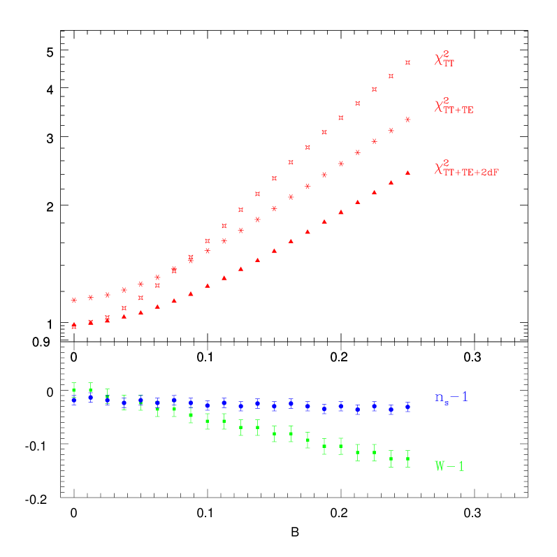
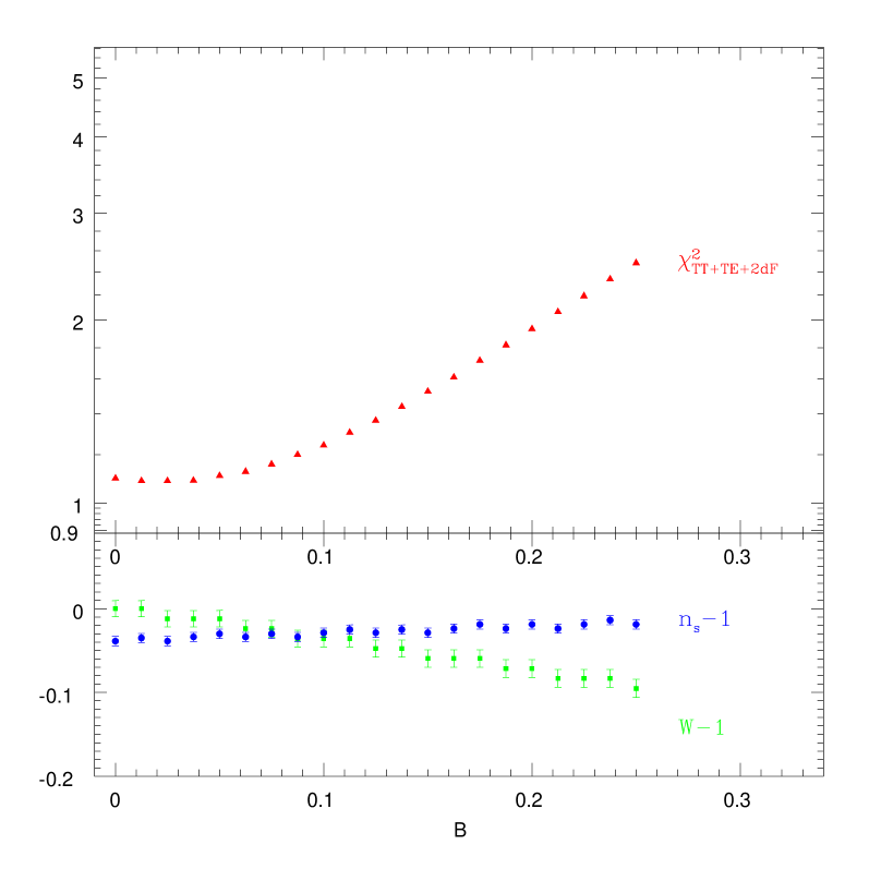
Figure 1: (Left) Minimum reduced $\chi^{2}/\nu$ as a function of $B$ for the fit of the $b$-free model to the WMAP’s TT (red triangles), TT+TE (red stars) and TT+TE+2dF (red hollow squares) with corresponding best fit values of $W-1$ (green squares) and $n_{s}-1$ (blue circles). We only show $W$ and $n_{s}$ from the fit to the TT data alone. The error bars correspond to the diagonal elements of the covariance matrix. Adding the remaining data sets changes the best fit values of $W$ and $n_{s}$ by only a small amount, well within the plotted error bar. (Right) Same as on the left but for the $b$-fixed model with all data sets included. In the left panel, $\nu=93$ and in the right $\nu=94$. The values of the reduced $\chi^{2}/\nu$ at $B=0$ are, in the left panel, 0.97 (TT), 1.1 (TT$+$TE) and 0.98 (TT$+$TE$+$2dF), and 1.1 in the right panel.

The left panel of Fig. 1, corresponding to the $b$-free model, contains plots of the minimized reduced $\chi^{2}_{\rm TT}/\nu$, $\chi^{2}_{\rm TT+TE}/\nu$ and $\chi^{2}_{\rm TT+TE+2dFa/}\nu$ ($\nu=93$) as functions of $B$ computed using, respectively, WMAP’s TT spectrum only, TT and TE, and TT, TE and the 2dF spectrum. As one can see from that plot, in all cases the lowest value of the minimum $\chi^{2}(B)/\nu$ occurs at $B=0$, i. e. when there is no contribution from strings. However, as additional data sets are added to the fit, the values of the minimum $\chi^{2}(B)$ become smaller. Fig. 1 also shows the values of $n_{s}-1$ and $W-1$ values that minimized $\chi^{2}/\nu$ at each $B$, with estimated uncertainties, of order $\pm 0.01$ for both. Not plotted are the values of the bias parameter $b$, which varied from 0.97 at $B=0$ to 1.02 at $B=0.25$. Note that the value of $n_{s}-1$ is typically around $-0.02\pm 0.01$ for $B\lesssim 0.1$, the region where the minimum $\chi^{2}(B)/\nu$ is less than about $1.25$.

The right panel of Fig. 1 corresponds to the $b$-fixed model, i. e. the model in which the value of the bias was held fixed at $b=\Omega_{m}^{0.6}/\beta$. Results are shown for the minimum value of $\chi^{2}(B)/\nu$ constructed using all three data sets. Here we find that the lowest value of the minimum $\chi^{2}(B)/\nu$ is at $B=0.025$, not $B=0$. In view of the limitations of our statistical analysis, one cannot attach much significance to either the existence of this minimum, or the precise nonzero $B$ at which it occurs, but it is worth observing that adding a small string contribution may be welcome when matching the CMBR normalized matter spectra to the galaxy data. Moreover, this result shows that at the very least we cannot exclude values of $B\sim 0.025$. We note that the values of $n_{s}-1$ corresponding to the minimum $\chi^{2}$ per degree of freedom grow with $B$ in this panel and, for $B\lesssim 0.1$, they fall within the range $n_{s}-1=-0.03\pm 0.01$.

In Figures 2 and 3 we plot the adiabatic plus string CMB and matter power spectra superposed using Eq. (43) with different values of $B$ and corresponding best fit values of $n_{s}$ and $W$ for the $b$-free and $b$-fixed models. In both figures, the solid line corresponds to $B=0$ and the dash-dot line to $(W=0,B=1)$.

Figure 2: (Left) Plots of the best fit $C_{l}^{TT}$ and $C_{l}^{TE}$ computed using the $b$-free model for different values of $B$ together with the WMAP’s binned data. (Right) Corresponding plots of the galaxy clustering power spectra together with the 2dFGRS data. On both plots, the solid line corresponds to $B=0$, dotted line - $B=0.05$, short dash line - $B=0.1$, long dash line - $B=0.15$ and the dash-dot line corresponds to the pure string contribution, i.e. $(W=0,B=1)$.

Figure 3: Same as in Fig. 2 but for the $b$-fixed model.

The simple adiabatic $\Lambda$CDM model with a constant $n_{s}$ fits the WMAP data very well in general, but much worse so on very large scales. For the first few multipoles, $2\leq l\leq 6$, the experiment finds a clear deficit of power, as compared to the prediction of the model. One could hope that, because cosmic strings generically predict such lack of power for low multipoles, adding a string component would improve the fit on large scales. However, as one can see from Figs. 2 and 3, this is not the case. The reason is that cosmic strings fit the data extremely poorly in the region of the first and the second acoustic peaks, where the WMAP error bars on $C_{l}$s are very small. The “benefit” from adding strings on larger scales, where the error bars are large, is offset by the much larger “damage” that strings cause when fitting on smaller scales.

Clearly, our partial statistical analysis does not yield a rigorous bound on the magnitude of $B$. However, the results in Fig. 1 can be used to get a rough estimate for the allowed range of the $B$ values. From the discussion at the start of this section, a reasonable bound can be based on taking $\chi^{2}(B)/\chi^{2}(0)\lesssim 1.25$. In Fig. 1, the maximum value of $B$ corresponding to this criterion would be $B_{max}\sim 0.1$. Moreover, we saw that the actual minimum value of $\chi^{2}(B)$ in the right panel of Fig. 1 was at $B\simeq 0.025$, not zero, which indicates that, almost certainly, the available data cannot exclude values of $B\lesssim 0.025$. As discussed in § III.1, this does not simply translate into a constraint on the value of the string tension, $G\mu$. Instead, from Eq. (55), $B\propto(G\mu^{/}\lambda)^{2}$.

Because cosmic strings produce a sizeable vector perturbation, in addition to the $E$-polarization, they can also induce the $B$-type polarization of the CMBR. In Fig. 4 we plot the $B$-polarization angular spectrum, $C_{l}^{BB}$, as predicted by our model with $B=0.1$. It appears that, even if cosmic strings were contributing only a few percent to the CMB temperature anisotropy, they could contribute a B-mode signal on scales $l\sim 800$ that would be in excess of the expected B-mode produced by lensing of the E-mode by galaxies lensing . Such a detection would be an important test for the existence of cosmic strings.

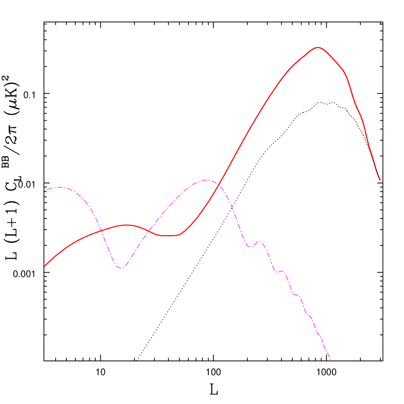
Figure 4: The $B$-type polarization spectrum $C_{l}^{BB}$ due to cosmic strings as predicted by our string model with the fit parameter $B$ set to $0.1$ is plotted as a solid red line. The expected $C_{l}^{BB}$ spectra for E to B lensing (dotted black line) and from primordial gravitational waves assuming a tensor-to-scalar ratio of $r=0.1$ (dash-dotted magenta line) are plotted for comparison.

IV Discussion

Cosmic strings appear to be a likely by-product of inflation in superstring cosmology. Although these cosmological models are only just beginning to be developed in sufficient detail for comparisons with data to be possible, most models seem to feature a string scale comparable to or slightly smaller than the GUT scale, and cosmic string tensions $G\mu\sim 10^{-10}-10^{-6}$.

These expectations motivate studying models in which CMB fluctuations and large scale structure are the consequence of both growing modes associated with perturbations generated from quantum fluctuations during inflation, and active perturbations associated with the gravitational effects of a network of cosmic strings. Here, we have presented an attempt at such an analysis, based on a rough comparison of theoretical models with both adiabatic perturbations and cosmic strings with WMAP TT and TE power spectra as well as the 2dFGRS results on galaxy correlation functions. Our results need to be improved in various ways, both by allowing numerous cosmological parameters we held fixed to vary, and by computing likelihood functions, rather than using a rough criterion based on a reduced $\chi^{2}$ statistic. Nevertheless, they already indicate that although the data currently available generally favor models without cosmic strings, they may not exclude nonzero cosmic string tension and density definitively, provided the growth of fluctuations in the Universe is not dominated by cosmic strings. Rather conservatively, we have argued that values of $B\lesssim 0.1$ are not excluded, although this result needs to be put on firmer footing statistically; we are quite confident that $B\lesssim 0.025$ cannot be excluded as yet. Since $\sqrt{B}\simeq(0.25/\lambda)(G\mu/1.1\times 10^{-6})$, these values of $B$ would correspond to

$$G\mu\lesssim{3.5\times 10^{-7}{\lambda\over 0.25}\sqrt{B\over 0.1}}~{}.$$ (59)

We have also found the values of $n_{s}-1$ that minimze the reduced $\chi^{2}$ statistic for different values of $B$. Conservatively, for the range $B\lesssim 0.1$, the various different comparisons with data in the two panels of Fig. 1 are consistent with $n_{s}-1\simeq-(0.04-0.01)$. Comparing with the predictions of various brane inflation models via Eqs. (9), (24) and (32), we note that the values we find are in agreement and certainly not in conflict with any of the models. However, we note that the Coulombic inflation models generally predict $|n_{s}-1|\lesssim-0.03$, at the low end of the range of values we infer from comparing with the data, while the powerlaw models allow larger $|n_{s}-1|$; Eq. (24) implies $|n_{s}-1|\gtrsim 0.03$ for any value of $\sigma$, and Eq. (32) implies a constant powerlaw index whose value depends on parameters of the brane inflation model. If $n_{s}(k)$ can be pinned down with greater precision, it may become possible to discriminate among different brane inflation models. We caution, though, since we have not varied the background cosmological model in obtaining these bounds, we cannot rule out that a more complete analysis would allow still larger values of $G\mu$, with other values of $n_{s}-1$. In a future publication we intend to present results of a more comprehensive study which would include varying all cosmological parameters as well as the relevant parameters of the string model, including their specific predictions for $n_{s}(k)$, and a better justified statistical analysis based on codes made available by the WMAP team for computing likelihood functions for any model for the production of temperature pertubations wmap_verde . (Some modifications will be needed to account for the nongaussianity of the cosmic string perturbations.) In addition to the WMAP and the 2dFGRS data, the analysis will also include the latest results from the Sload Digital Sky Survey (SDSS) sloan .

The key to our analysis is the idea that the Universe is a patchwork quilt, with a little bit of cosmic strings thrown in to complicate the models. A smoking gun for the existence of cosmic strings could be the detection of B-mode polarization on smaller scales at an amplitude considerably larger than is predicted in inflation models without cosmic strings. Another potentially distinguishing signature of cosmic strings could be the detection of cosmological non-Gaussianity. Tests of the WMAP data wmap_komatsu have so far been limited to constraining the type of non-Gaussianity expected from inflationary models. Some of the most commonly used tests of non-Gaussianity, such as the bispectrum test, had actually been shown to be insensitive to possible contributions from cosmic strings gangui . Specially tailored tests are likely to be needed to detect string induced non-Gaussianity proty . Cosmic strings may also be detected from the observation of identical galaxy pairs in close proximity on the sky galaxypairs . Gravitational radiation from kinks in cosmic strings may also be detectable down to exceptionally small values of $G\mu$ vil-dam . Pulsar timing is likely to push bounds on the density in long wavelength gravitational radiation backgrounds kaspi down by an order of magnitude or so, corresponding to a factor of three or so in $G\mu/\lambda^{2}$ backer , but a substantial contribution to the background from supermassive black hole binaries jaffe may frustrate our ability to use these observations to constrain the cosmic string tension much further.