Towards a Stringy Resolution of the Cosmological Singularity

Abstract

We study cosmological solutions to the low-energy effective action of heterotic string theory including possible leading order $\alpha^{\prime}$ corrections and a potential for the dilaton. We consider the possibility that including such stringy corrections can resolve the initial cosmological singularity. Since the exact form of these corrections is not known the higher-derivative terms are constructed so that they vanish when the metric is de Sitter spacetime. The constructed terms are compatible with known restrictions from scattering amplitude and string worldsheet beta-function calculations. Analytic and numerical techniques are used to construct a singularity-free cosmological solution. At late times and low-curvatures the metric is asymptotically Minkowski and the dilaton is frozen. In the high-curvature regime the universe enters a de Sitter phase.

I Introduction

Arguably, the most perplexing problem of modern cosmology is the initial singularity problem. The theorems of Hawking and Penrose state that many of the manifolds of General Relativity are geodesically incomplete Hawking:1969sw . In particular, many solutions to the Friedmann-Robertson-Walker (FRW) isotropic and homogeneous model of the universe contain singularities. In order to gain a complete description of the early universe a theory of quantum gravity is required. In general, it is believed that such a theory may somehow resolve the initial singularity allowing us to obtain well-defined, finite solutions to calculations of physical quantities.

Superstring theory is currently the best candidate for a theory of quantum gravity. It is therefore only natural to try to use string theory to probe the very early universe. Many of us are hopeful that string theory (or M-theory) will lead to a consistent cosmological model capable of resolving the initial singularity . We are inspired, in part, by the ability of stringy physics to resolve certain singularities in time-independent orbifolds and conifolds Liu:2002yd -Greene:1995hu . A full understanding of the initial singularity problem will most likely require nonperturbative physics, and most certainly will require a better understanding of time-dependent solutions in string theory.

In this paper we provide a toy model of a nonsingular FRW cosmology, based on string theory. Our goal is to discuss only one possible way in which string theory may begin to address the initial singularity problem. Our concrete starting point is the low-energy effective action of heterotic string theory including possible leading order $\alpha^{\prime}$ corrections . While the exact structure of these corrections is not known, we provide an example in which the resulting cosmology is singularity-free . To study the system we use both analytic and numerical techniques. The metric is asymptotically Minkowski spacetime at low-curvatures and evolves to de Sitter space in the high-curvature regime. The significance of the $\alpha^{\prime}$ corrections is controlled, in part, by the dilaton field $\Phi$. These higher-derivative terms become important in the high-curvature regime and are constructed to allow de Sitter solutions in the early universe. In this way our model provides the first natural realization of the Limiting Curvature Construction (LCC) in terms of a well-motivated, physical theory markov -easson2003 . Our analysis involves a dynamical dilaton and a novel, string-inspired form for the higher-derivative terms.

II The Action

In $D$-dimensions, the string tree-level effective action for the massless boson sector (in the string-frame) is:

$$\tilde{S} = \frac{M_{\rm s}^{D-2}}{2}\int d^{D}\!x\sqrt{-\tilde{g}}\,e^{-2\Phi}\,\Big{\{}\,\tilde{R}\,+\,4(\nabla\Phi)^{2}$$ (2.1)

$$+ \zeta_{0}\alpha^{\prime}\,\tilde{\mathcal{L}}_{2}\,-\frac{2(D-10)}{3\alpha^{\prime}}+{\mathcal{O}}(a^{\prime 2}\tilde{R}^{4}+\cdots)\,\Big{\}}$$

where $\Phi$ is the dilaton, $\alpha^{\prime}=\ell_{\rm s}^{2}$ and the tilde indicates that we are using the string-frame metric $\tilde{g}_{MN}$, where $M,N=0,\dots,d$. In the above, $\zeta_{0}$ takes on the values $1/4,\,1/8,\,0$ for the bosonic, heterotic and type II superstring theories, respectively. The “$\cdots$” refer to other higher-derivative terms of order $\alpha^{\prime 2}$, and the Lagrangian $\tilde{\mathcal{L}}_{2}$ represents the leading-order corrections to the action and is made up of four-derivative terms $\tilde{\mathcal{L}}_{2}(\tilde{R}^{2},\,\tilde{R}_{\mu\nu}\tilde{R}^{\mu\nu},\,\tilde{R}_{\mu\nu\lambda\sigma}\tilde{R}^{\mu\nu\lambda\sigma},\dots)$ Gross:1986mw ; Metsaev:1987zx . We choose to work within heterotic sting theory. While the two-point action for the heterotic string includes a gauge vector boson $A_{n}$ (with field strength tensor $F_{mn}$) and an anti-symmetric tensor $H_{abc}$:

$${\mathcal{L}}_{2pt} = \frac{1}{2\kappa^{2}}\,R\,-\,\frac{1}{6}\,e^{-2\Phi}\,H_{abc}H^{abc}\,-\,{1\over 2}\,(\nabla_{c}\Phi)(\nabla^{c}\Phi)$$ (2.2)

$$\,-\, \frac{1}{4}\,e^{-\Phi}\,F_{mn}F^{mn}$$

we consider only the most relevant massless modes, the dilaton $\Phi$ and graviton $g_{mn}$. In order to obtain results that are easy to compare with General Relativistic theory we work in the Einstein-frame obtained via a conformal transformation of the metric $\tilde{g}_{\alpha\beta}=e^{\xi\Phi}g_{\alpha\beta}$. Applying this transformation to (2.1) gives the Einstein-frame action

$$S = \frac{M_{\rm s}^{D-2}}{2}\int d^{D}\!x\sqrt{-g}\,\Big{\{}\,R\,-\,\xi(\nabla\Phi)^{2}$$ (2.3)

$$+ \zeta_{0}\alpha^{\prime}e^{-\xi\Phi}\,\Big{[}\mathcal{L}_{2}\,+\,\xi^{2}\frac{D-4}{D-2}(\nabla\Phi)^{4}\Big{]}\,-\Lambda e^{\xi\Phi}$$

$$+ {\mathcal{O}}(a^{\prime 2}R^{4}+\cdots\,)\,\Big{\}}\,,$$

where $\xi=4/(D-2)$ and $\Lambda=2(D-10)/3\alpha^{\prime}$ is a contribution to the cosmological constant that vanishes in ten-dimensions. In the Einstein-frame the dilaton couples directly to the higher-derivative terms $e^{-\xi\Phi}\mathcal{L}_{2}$. In this way it is possible to control the “strength” of the $\mathcal{L}_{2}$ terms, in part, via the dilaton.

Our knowledge of the exact form of $\mathcal{L}_{2}$ is incomplete. Requiring the action to reproduce string theory S-matrix elements can determine only some of the coefficients of potential covariant terms in $\mathcal{L}_{2}$. This is because some terms do not contribute to the S-matrix or provide contributions that overlap in form with those of other terms Metsaev:1987zx ; Forger:1996vj . Some sort of off-shell superstring calculation is required to fix the exact coefficients of these terms. Scattering amplitude or string worldsheet $\beta$-function calculations predict only the Riemann squared term $R_{\mu\nu\lambda\sigma}R^{\mu\nu\lambda\sigma}$ in $\mathcal{L}_{2}$. In Metsaev:1987zx Metsaev and Tseytlin fix the contribution

$$\bar{\mathcal{L}}_{2}\,=\,\zeta_{0}\,e^{-2\Phi}\,\left(R_{\mu\nu\lambda\sigma}R^{\mu\nu\lambda\sigma}\,+\,\xi^{2}\,\frac{D-4}{D-2}\,(\nabla\Phi)^{4}\,\right)\,,$$ (2.4)

where $\bar{\mathcal{L}}_{2}$ is the term being multiplied by $\alpha^{\prime}$ in (2.3). However, terms such as $R^{2}$ and $R_{\mu\nu}R^{\mu\nu}$ may be added and subtracted from $\mathcal{L}_{2}$ by performing field redefinitions of ${\mathcal{L}}_{2pt}$ Gross:1986mw . Because of this imprecise knowledge of $\mathcal{L}_{2}$, $\mathcal{L}_{2}$ is commonly assumed to be the Gauss-Bonnet invariant

$${\mathcal{L}}_{GB}=R_{\mu\nu\lambda\sigma}R^{\mu\nu\lambda\sigma}\,-\,4\,R_{\mu\nu}R^{\mu\nu}\,+\,R^{2}\,.$$ (2.5)

An advantage of choosing this particular structure for $\mathcal{L}_{2}$ is that the resulting equations of motion are second-order. The cost of choosing an invariant of a form other than (2.5) is that our equations of motion will be fourth-order. Because we are interested in finding a nonsingular theory we will design something other than the Gauss-Bonnet form for $\mathcal{L}_{2}$ . A simple way to ensure that our theory has a nonsingular solution is to choose an $\mathcal{L}_{2}$ that will vanish for a nonsingular spacetime. We can then look for solutions that approach this nonsingular manifold in the large curvature regime. As predicted by the string theory calculation (2.4), we take the leading term in $\mathcal{L}_{2}$ to be $R_{\mu\nu\lambda\sigma}R^{\mu\nu\lambda\sigma}$. An elementary set of nonsingular spacetimes are the set of maximally symmetric spacetimes of constant curvature. The metrics of constant curvature are locally characterized by the condition (in $D=4$)

$$R_{\alpha\beta\gamma\delta}=\frac{1}{12}\,R\,(\,g_{\alpha\gamma}g_{\beta\delta}\,-\,g_{\alpha\delta}g_{\beta\gamma}\,)\,,$$ (2.6)

which is equivalent to

$$C_{\alpha\beta\gamma\delta}\,=\,0\,=\,R_{\alpha\beta}\,-\,\frac{1}{4}\,R\,g_{\alpha\beta}\,.$$ (2.7)

The space with constant curvature and $R=0$ is Minkowski spacetime. The space for $R>0$ is de Sitter spacetime, which has topology ${\mathbf{R}}^{1}\times{\mathbf{S}}^{3}$. The space with $R<0$ is anti-de Sitter spacetime, which has topology ${\mathbf{S}}^{1}\times{\mathbf{R}}^{3}$.

Using equation (2.6) it is easy to construct the desired invariant that will vanish for spacetimes of constant curvature (in $D=4$) and whose leading term is $R_{\mu\nu\lambda\sigma}R^{\mu\nu\lambda\sigma}$:

$$\mathcal{L}_{2}\,=\,R_{\mu\nu\lambda\sigma}R^{\mu\nu\lambda\sigma}-\frac{1}{6}R^{2}\,.$$ (2.8)

Note that it is possible that there are other solutions satisfying $\mathcal{L}_{2}=0$ (see [47]). This is a limitation of the construction as presented. If there are other solutions satisfying this condition then we could try to modify this Lagrangian so that these solution no longer obey this condition. However, we are not primarily interested in finding all the solutions to this theory. Our main goal is to show only that nonsingular solutions of the type described above exist. The four-dimensional action is given by equation (2.3), and may be written

$$S = \frac{M_{\rm s}^{2}}{2}\int d^{4}\!x\sqrt{-g}\,\Big{\{}\,R\,-\,2(\nabla\Phi)^{2}$$ (2.9)

$$+ D(\Phi)\,\Big{[}R_{\mu\nu\lambda\sigma}R^{\mu\nu\lambda\sigma}-\frac{1}{6}R^{2}\Big{]}\,-V(\Phi)\Big{\}}\,,$$

where $D(\Phi)=\alpha^{\prime}e^{-2\Phi}/8$. In the above we have assumed a potential for the dilaton field $V(\Phi)$ and we have ignored the contribution to the cosmological constant term, $\Lambda e^{2\Phi}$ (i.e. we do not attempt to solve the cosmological constant problem). We will comment further on the dilaton potential below.

Variation of the action with respect to the metric tensor yields:

$$4(R_{;\beta}\,D(\Phi)_{;\alpha}\,+R_{;\alpha}\,D(\Phi)_{;\beta}+D(\Phi)_{;\gamma}\,(12\,R_{\alpha\beta;}{}{}^{\gamma}-6(R_{\alpha}{}^{\gamma}{}_{;\beta}+R_{\beta}{}^{\gamma}{}_{;\alpha})-R_{;}{}^{\gamma}\,g_{\alpha\beta}))+2(2R\,D(\Phi)_{;\alpha\beta}$$ (2.10)

$$+ 2(-5\,R_{;\alpha\beta}\,+\,+6(R_{\alpha\beta;\gamma}{}^{\gamma}\,+\,R_{\alpha\beta;}{}^{\gamma}{}_{\gamma}))\,D(\Phi)-3(R\,-\,2\Phi_{;\gamma}\Phi_{;}{}^{\gamma})g_{\alpha\beta}+6(R_{\alpha\beta}\,+\,2D(\Phi)_{;}{}^{\gamma\lambda}R_{\gamma\beta\lambda\alpha}$$

$$+ 2D(\Phi)_{;\gamma\lambda}R_{\alpha}{}^{\lambda}{}_{\beta}{}^{\gamma}))+D(\Phi)(-4(RR_{\alpha\beta}+12R_{\gamma\beta}R_{\alpha}{}^{\gamma}-12R_{\gamma\lambda}R_{\alpha}{}^{\gamma}{}_{\beta}{}^{\lambda}+6R_{\gamma\lambda\rho\alpha}R_{\beta}{}^{\rho\gamma\lambda})$$

$$+ g_{\alpha\beta}(R^{2}-4R_{;\gamma}{}^{\gamma}-6R_{\gamma\lambda\rho\sigma}R^{\gamma\lambda\rho\sigma}))+6g_{\alpha\beta}V(\Phi)$$

$$\,=\, 4RD(\Phi)_{;}{}^{\gamma}{}_{\gamma}\,g_{\alpha\beta}\,+\,4D(\Phi)_{;}{}^{\gamma}\,(6(R_{\gamma\alpha;\beta}\,+\,R_{\gamma\beta;\alpha}-2R_{\alpha\beta;\gamma})\,+\,R_{;\gamma}g_{\alpha\beta})\,,$$

while variation with respect to the field $\Phi$ gives

$$\sqrt{-g}\Big{(}(R_{\mu\nu\lambda\sigma}R^{\mu\nu\lambda\sigma}-\frac{1}{6}R^{2})\frac{\partial D(\Phi)}{\partial\Phi}+4\nabla^{2}\Phi\Big{)}$$ (2.11)

$$= \sqrt{-g}\frac{\partial V(\Phi)}{\partial\Phi}\,.$$

III Cosmological solutions

We now study cosmological solutions to the theory (2.9). We assume a time-dependent FRW homogeneous and isotropic metric

$$ds^{2}=-n^{2}(t)dt^{2}+a^{2}(t)\left[\frac{dr^{2}}{1-k{r^{2}}}+r^{2}d{\theta}^{2}+r^{2}\sin^{2}{\theta}d\varphi^{2}\right]$$ (3.12)

where $a(t)$ is the scale factor of the universe and $n(t)$ is the lapse function. For simplicity we take the metric to be flat ($k=0$). We also choose a time-dependent, homogeneous dilaton $\Phi(t)$. An alternative derivation of the equations of motion (2.10) and (2.11) is achieved by substituting the metric (3.12) into (2.9) and varying the action with respect to $a$, $n$, and $\Phi$. The resulting EOM are:

$$e^{2\Phi}a^{4}(V(\Phi)\,-\,2\dot{\Phi}^{2})=6\lambda\dot{a}^{4} + 8\lambda a\dot{a}^{2}(\,2\dot{a}\dot{\Phi}\,-\,3\ddot{a}\,)+2a^{2}(\,3\lambda\ddot{a}^{2}\,+\,\dot{a}^{2}(\,e^{2\Phi}\,-\,8\lambda\dot{\Phi}^{2}\,+\,4\lambda\ddot{\Phi}\,)$$ (3.13)

$$+ 4\lambda\dot{a}\,\,\ddot{}\!a\dot{}\,)+4a^{3}(\ddot{a}(e^{2\Phi}+4\lambda\dot{\Phi}^{2}-2\lambda\ddot{\Phi})+\lambda(-4\dot{\Phi}\,\,\ddot{}\!a\dot{}\,+\,\ddot{}\!a\ddot{}\,))$$

$$18\lambda\dot{a}^{4}+e^{2\Phi}a^{4}(V(\Phi)+2\dot{\Phi}^{2}) = 6a(2\lambda\dot{a}^{2}(2\dot{a}\dot{\Phi}+\ddot{a})+a(e^{2\Phi}\dot{a}^{2}-\lambda\ddot{a}^{2}+2\lambda\dot{a}(-2\dot{\Phi}\ddot{a}+\,\ddot{}\!a\dot{}\,)))$$ (3.14)

$$12\lambda(\,\dot{a}^{2}\,-\,a\ddot{a}\,)^{2} + e^{2\Phi}a^{3}\,(\,12\dot{a}\dot{\Phi}\,+\,a(\,V^{\prime}(\Phi)\,+\,4\ddot{\Phi}\,)\,)\,=\,0\,,$$ (3.15)

where $\lambda=\alpha^{\prime}/8$ and the prime in the last equation denotes differentiation with respect to $\Phi$. In the above we have set $n=1$. Note that the dynamics of this system are completely determined by the $G_{00}$ equation (3.14) and the EOM for the scalar field (3.15). Equation (3.13) serves as a constraint equation. To reduce these equations to a second-order system, introduce $H=\dot{a}/a$. Equations (3.14) and (3.15) reduce to

$$\dot{H}^{2} - 2H\ddot{H}-6H^{2}\dot{H}+4H\dot{H}\dot{\Phi}$$ (3.16)

$$= -\frac{e^{2\Phi}}{6\lambda}\left(V(\Phi)+2\dot{\Phi}^{2}-6\lambda H^{2}\right)$$

$$12\lambda\dot{H}^{2} = -e^{2\Phi}\left(\frac{\partial V(\Phi)}{\partial\Phi}+4\ddot{\Phi}+12H\dot{\Phi}\right)\,,$$ (3.17)

III.1 The late-time universe

At late times (low curvatures) our action must mimic General Relativity and the Einstein-Hilbert action $S_{EH}=(1/2\kappa^{2})\int d^{4}x\sqrt{-g}\,R\,.$ This implies the contribution $D(\Phi)\mathcal{L}_{2}-2(\nabla\Phi)^{2}-V(\Phi)$ in equation (2.9) must not produce any physical deviations from $S_{EH}$ in the low-curvature regime. Furthermore, the dilaton must approach a $\Phi\mapsto\Phi_{0}$. If the dilaton remained time-dependent it would produce observational consequences such as variations in gauge-couplings. We also demand $V(\Phi)\mapsto 0$ to avoid gaining a contribution to the cosmological constant in the late universe. A de Sitter space solution $a(t)=a_{0}\exp{Ht}$ corresponds to constant $H=H_{0}$. In the case under consideration ($V(\Phi)\mapsto 0$, $\Phi\mapsto\Phi_{0}$) the EOM are satisfied by a de Sitter solution with the constraint $H=0$ and hence, $a(t)=const$. Therefore, in the (late-time) case of constant dilaton and vanishing potential the equations of motion are solved by Minkowski spacetime (the special case of de Sitter with $H=0$) with flat metric $g_{\alpha\beta}=\eta_{\alpha\beta}=diag(-1,1,1,1)$.

III.2 The early universe

In order to remove the initial Big-Bang curvature singularity present in Einstein gravity at $t=0$, the term $\mathcal{L}_{2}$ must become significant. This will force the metric solution to de Sitter spacetime with metric (3.12) and $a(t)\propto\exp{Ht}$. Discovering a solution which evolves smoothly from a de Sitter phase at early times to Minkowski at late times will provide an example of a universe which is everywhere nonsingular. We now produce such a solution and proceed to study its stability against classical perturbations. Simple forms for $\Phi$ and $V(\Phi)$ that provide the desired behavior and obey the EOM are

$$\Phi(t)=\Phi_{0}\tanh{\left(\frac{t-t_{1}}{t_{0}}\right)}\,,$$ (3.18)

and

$$V(\Phi)=V_{0}\left((\Phi+1)^{2}-4\right)\,,$$ (3.19)

where we set $\Phi_{0}=1$, $V_{0}=-3H_{0}^{2}/2$ and $t_{0}=1$. The constant $t_{1}$ is taken to be large enough so that $\Phi(t=0)\approx-1$. Note that the potential (3.19) is everywhere positive for all allowed values of the dilaton $\Phi$ (over the range, $(-1,1)$) and hence, for all time $t\in(-\infty,\infty)$ (see Fig.1).

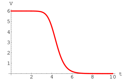
Figure 1: The time evolution of the potential $V(\Phi)$. For this plot (and all subsequent plots) we take $t_{1}=4$ and $H_{0}=1$.

The choices for $\Phi$ and $V$ are certainly not unique. Any $\Phi$ and $V$ that have the correct asymptotic behavior have the potential to generate nonsingular solutions of the type under consideration. Inserting the $\Phi$ ansatz (3.18) and the $V$ ansatz (3.19) into the EOM (equations (3.13) to (3.15)) we find that as $t\mapsto 0$, $a(t)\propto\exp{Ht}$ (in our specific example $H_{0}=1$). At late times the metric approaches flat Minkowski space.

III.3 Numerical analysis

While we have shown that our solution has the desired asymptotic behavior, namely, de Sitter space at early times and Minkowski space at late times, we must prove that this solution remains nonsingular for all values of $t$ in between. To do this we conduct a numerical study of the equations of motion. Consider the phase space generated by the equations (3.14) and (3.15) with $\Phi$ and $V$ given by (3.18) and (3.19). The $(\Phi,H)$-plane is plotted in Fig.2. Note that the range of $\Phi$, $(-1,1)$ is mapped to the entire history of the universe $t\in(-\infty,\infty)$.

Clearly, the curvature is bounded for all time and therefore, the universe is free of curvature singularities. At early times ($\Phi\mapsto-1$) the curvature $|H|$ is approximately a positive constant corresponding to the de Sitter phase. At late times the dilaton approaches a constant ($\Phi\mapsto 1$), the curvature vanishes and the spacetime approaches flat Minkowski space. Of course, recent observational evidence from supernovae data Riess:1998cb and the WMAP satellite Spergel:2003cb indicate that the universe is not only expanding but undergoing an accelerated expansion. It is easy to modify the Minkowski condition in this model in order to accommodate various late time behaviors (for example, by adding an appropriate matter Lagrangian to the system). To achieve an accelerating universe at late times one simply could tune the potential to not go exactly to zero at late times like in quintessence models.

It is important to discuss the stability of this solution. We now show that this solution is not (in general) an attractor at early times but is at late times. Therefore, nonsingular solutions of the type described here are not generic in the model under consideration. It is possible, however, that other nonsingular solutions exist in this theory that are attractors. Furthermore, as pointed out by Starobinsky starob , the evolution of the Universe need not follow a generic solution, it may well be described just by this unique one, at least initially. The late time behavior of Minkowski spacetime with frozen dilaton is classically stable against small perturbations. Let us begin with the stability analysis of the early-time solution. For our considerations it is sufficient to consider stability against homogeneous fluctuations. An analysis of inhomogeneous fluctuations is considerably more involved.

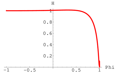
Figure 2: The $(\Phi,H)$-phase portrait generated from the equations of motion. Note that the curvature remains finite for the entire history of the universe.

Let

$$a(t)=a_{0}e^{Ht}\left(1+\delta(t)\right),\qquad|\delta(t)|<<1\,.$$ (3.20)

$$\Phi(t)=\Phi_{0}\tanh{\left(\frac{t-t_{1}}{t_{0}}\right)}\left(1+\epsilon(t)\right),\qquad|\epsilon(t)|<<1\,.$$ (3.21)

Recall, that when $t\mapsto 0$, $\Phi\mapsto-1$. To first approximation in $\delta$ and $\epsilon$ the $G_{00}$ equation and the equation of motion for $\Phi$ become

$$\ddot{\delta} + 3H\dot{\delta}+\frac{\delta}{\lambda e^{2}}=0\,$$ (3.22)

$$4\ddot{\epsilon} + 12H\dot{\epsilon}=3H^{2}\epsilon\,.$$ (3.23)

The solutions to these equations are

$$\delta=\frac{d_{1}+d_{2}\,e^{\frac{\sqrt{9\lambda e^{2}H^{2}-4}\,t}{\lambda^{1/2}e}}}{\exp{(((3He+\frac{\sqrt{9\lambda e^{2}H^{2}-4}}{\lambda^{1/2}}))t/2e)}}$$ (3.24)

$$\epsilon=\frac{c_{1}+c_{2}\,e^{2\sqrt{3}\,Ht}}{e^{((3+2\sqrt{3})\,Ht)/2}}\,.$$ (3.25)

Here $d_{1}$, $d_{2}$, $c_{1}$ and $c_{2}$ are constants. The conditions that $\epsilon$ and $\delta$ be small ($<<1$) at the beginning of our analysis when $t\simeq 0$ implies that $|c_{1}+c_{2}|<<1$ and $|d_{1}+d_{2}|<<1$. While $\delta$ remains small for all time (for small $d_{1}$ and $d_{2}$) $\epsilon$, in general, grows greater than unity and our solution becomes unstable . Hence, at early times the solution is stable against perturbations of the metric but not against perturbations of the dilaton $\Phi$. This demonstrates that nonsingular solutions of the type given above are not generic.

To see if the late-time Minkowski space solution is stable we consider perturbations around the Minkowski solution

$$a(t)=a_{0}\left(1+\delta(t)\right),\qquad|\delta(t)|<<1\,,$$ (3.26)

and perturbations of the dilaton of the form (3.21). Recall that at late times (as $t\mapsto\infty$), $\Phi\mapsto 1$. To first approximation in $\delta$ and $\epsilon$ the $G_{00}$ and the equation of motion for $\Phi$ give $\delta=\epsilon=0$. Therefore, our late-time Minkowski space solution is an attractor.

IV Conclusions

In this letter we studied cosmological solutions to heterotic string theory including a possible form for leading order $\alpha^{\prime}$ corrections to the low-energy effective action. A nonsingular solution is given in which the universe evolves from an early-time de Sitter phase to a late-time Minkowski spacetime with constant dilaton. One limitation of this model is that at high-energies and large curvatures $E^{2}\alpha^{\prime}\simeq{\mathcal{O}}(1)$ higher-order curvature corrections (e.g. $\alpha^{\prime 2}$ corrections) become important. Including these terms or quantum loop corrections in $g_{\rm s}=e^{\left<\Phi\right>}$ could, presumably, re-introduce the singularity. Of course, if the string scale is TeV then such corrections will become important sooner then if the string scale is near the Planck scale. It is likely that a full nonperturbative analysis is required in order to fully understand the initial singularity problem. Our analysis is meant to show a possible way in which string theory may address this issue. We have shown that including higher-derivative terms in the action can (under certain circumstances) resolve the initial curvature singularity.

Finally, it would be interesting to see if this construction can regulate the bounce that occurs in the Pre-Big-Bang (PBB) model of string cosmology Veneziano:1991ek ; Gasperini:1992em . The analysis would involve ideas from this paper and from Brandenberger:1998zs ; Easson:1999xw . In the PBB model the universe starts out in the perturbative string Minkowski vacuum. The universe then goes through a high-curvature, collapsing regime during which the $\alpha^{\prime}$ corrections become important. Hopefully, after a successful “graceful exit”, the universe enters an expanding low-curvature radiation (or quintessence) dominated phase. In this paper we have studied only the post-collapse branch of the PBB model. The collapsing branch would be the time reverse of this. We leave a more detailed analysis of the PBB scenario in this context to a future paper.

- (1) S. W. Hawking and R. Penrose, Proc. Roy. Soc. Lond. A 314, 529 (1970).
- (2) R. H. Brandenberger and C. Vafa, Nucl. Phys. B 316, 391 (1989).
- (3) M. Sakellariadou, Nucl. Phys. B 468, 319 (1996) [arXiv:hep-th/9511075].
- (4) S. Alexander, R. H. Brandenberger and D. Easson, Phys. Rev. D 62, 103509 (2000) [hep-th/0005212].
- (5) R. Brandenberger, D. A. Easson and D. Kimberly, Nucl. Phys. B 623, 421 (2002) [arXiv:hep-th/0109165].
- (6) J. E. Lidsey, D. Wands and E. J. Copeland, Phys. Rept. 337, 343 (2000) [arXiv:hep-th/9909061].
- (7) D. A. Easson, Int. J. Mod. Phys. A 16, 4803 (2001) [arXiv:hep-th/0003086].
- (8) F. Quevedo, Class. Quant. Grav. 19, 5721 (2002) [arXiv:hep-th/0210292].
- (9) M. Gasperini and G. Veneziano, Phys. Rept. 373, 1 (2003) [arXiv:hep-th/0207130].
- (10) H. Liu, G. Moore and N. Seiberg, arXiv:gr-qc/0301001.
- (11) L. J. Dixon, J. A. Harvey, C. Vafa and E. Witten, Nucl. Phys. B 261, 678 (1985).
- (12) L. J. Dixon, J. A. Harvey, C. Vafa and E. Witten, Nucl. Phys. B 274, 285 (1986).
- (13) A. Strominger, Nucl. Phys. B 451, 96 (1995) [arXiv:hep-th/9504090].
- (14) B. R. Greene, D. R. Morrison and A. Strominger, Nucl. Phys. B 451, 109 (1995) [arXiv:hep-th/9504145].
- (15) I. Antoniadis, J. Rizos and K. Tamvakis, Nucl. Phys. B 415, 497 (1994) [arXiv:hep-th/9305025].
- (16) R. Brustein and R. Madden, Phys. Rev. D 57, 712 (1998) [arXiv:hep-th/9708046].
- (17) R. Brustein and R. Madden, Hadronic J. 21, 202 (1998) [arXiv:hep-th/9711134].
- (18) P. Kanti, J. Rizos and K. Tamvakis, Phys. Rev. D 59, 083512 (1999) [arXiv:gr-qc/9806085].
- (19) R. Brustein and R. Madden, JHEP 9907, 006 (1999) [arXiv:hep-th/9901044].
- (20) S. Davis, Gen. Rel. Grav. 32, 541 (2000) [arXiv:gr-qc/9911021].
- (21) S. Tsujikawa, Class. Quant. Grav. 20, 1991 (2003) [arXiv:hep-th/0302181].
- (22) S. W. Hawking and G.F.R. Ellis, “The large scale structure of space time,” , Cambridge University Press, Cambridge (1973).
- (23) G. T. Horowitz and A. R. Steif, Phys. Rev. Lett. 64, 260 (1990).
- (24) M. A. Markov, Pisma Zh. Eksp. Teor. Fiz. 36, 214 (1982); Pisma Zh. Eksp. Teor. Fiz. 46, 342 (1987).
- (25) V. P. Frolov, M. A. Markov and V. F. Mukhanov, Phys. Lett. B 216, 272 (1989).
- (26) V. P. Frolov, M. A. Markov and V. F. Mukhanov, Phys. Rev. D 41, 383 (1990).
- (27) V. Mukhanov and R. H. Brandenberger, Phys. Rev. Lett. 68, 1969 (1992).
- (28) M. Trodden, V. F. Mukhanov and R. H. Brandenberger, Phys. Lett. B 316, 483 (1993) [arXiv:hep-th/9305111].
- (29) R. H. Brandenberger, V. Mukhanov and A. Sornborger, Phys. Rev. D 48, 1629 (1993) [arXiv:gr-qc/9303001].
- (30) R. Moessner and M. Trodden, Phys. Rev. D 51, 2801 (1995) [arXiv:gr-qc/9405004].
- (31) R. H. Brandenberger, arXiv:gr-qc/9503001.
- (32) R. H. Brandenberger, R. Easther and J. Maia, JHEP 9808, 007 (1998) [arXiv:gr-qc/9806111].
- (33) D. A. Easson and R. H. Brandenberger, JHEP 9909, 003 (1999) [arXiv:hep-th/9905175].
- (34) D. A. Easson, “M-Theory And Superstring Cosmology: Brane Gases In The Early Universe And Nonsingular Gravity,” UMI-30-50883.
- (35) D. A. Easson, JHEP 0302, 037 (2003) [arXiv:hep-th/0210016].
- (36) D. A. Easson, P. Martineau and R. Brandenberger, “A Nonsingular Four-Dimensional Black Hole,” MCGILL-03-03, to appear on hep-th.
- (37) D. J. Gross and J. H. Sloan, Nucl. Phys. B 291, 41 (1987).
- (38) R. R. Metsaev and A. A. Tseytlin, Nucl. Phys. B 293, 385 (1987).
- (39) K. Forger, B. A. Ovrut, S. J. Theisen and D. Waldram, Phys. Lett. B 388, 512 (1996) [arXiv:hep-th/9605145].
- (40) A. G. Riess et al. [Supernova Search Team Collaboration], a Cosmological Constant,” Astron. J. 116, 1009 (1998) [arXiv:astro-ph/9805201].
- (41) D. N. Spergel et al., arXiv:astro-ph/0302209.
- (42) A. A. Starobinsky, Phys. Lett. B 91, 99 (1980).
- (43) G. Veneziano, Phys. Lett. B 265, 287 (1991).
- (44) M. Gasperini and G. Veneziano, Astropart. Phys. 1, 317 (1993) [arXiv:hep-th/9211021].