Sphalerons, spectral flow, and anomalies

Abstract

The topology of configuration space may be responsible in part for the existence of sphalerons. Here, sphalerons are defined to be static but unstable finite-energy solutions of the classical field equations. Another manifestation of the nontrivial topology of configuration space is the phenomenon of spectral flow for the eigenvalues of the Dirac Hamiltonian. The spectral flow, in turn, is related to the possible existence of anomalies. In this review, the interconnection of these topics is illustrated for three particular sphalerons of $SU(2)$ Yang–Mills–Higgs theory.
Invited paper for the special issue of the Journal of Mathematical Physics on “Integrability, topological solitons and beyond” edited by T. Fokas and N.S. Manton.

I Introduction

One of the main themes of the present special issue concerns the so-called topological solitons. The field configurations of these classical solutions are characterized by a topologically nontrivial map of the space manifold (or part of it) into some internal space of the model considered. A well-known example is the Skyrme soliton Sk60 , for which the space manifold $S^{3}$ (i.e., the compactified Euclidean space $\mathbb{R}^{3}$) is mapped into the internal space $SU(2)$. Another example is the magnetic monopole tHP74 , for which the “sphere at infinity” $S^{2}$ is mapped into the Higgs vacuum manifold $SO(3)/SO(2)$.

There exist, however, other classical solutions, the so-called sphalerons, which themselves have trivial topology but trace back to nontrivial topology in the configuration space of the fields T82 ; M83 . In this contribution, we intend to give an elementary discussion of sphaleron solutions in Yang–Mills–Higgs theory and the underlying topology. In order to get a clear picture of what goes on, we focus on a single Yang–Mills–Higgs theory and three specific sphalerons KM84 ; K93 ; KO94 .

Physically, the topological solitons and the sphalerons play a different role. Solitons are primarily relevant to the equilibrium properties of the theory (e.g., the existence of certain stable asymptotic states), whereas sphalerons are of importance to the dynamics of the theory. The sphaleron KM84 of the electroweak Standard Model EWSM , for example, is believed to play a crucial role for baryon-number-violating processes in the early universe (see, e.g., Refs. McL94 ; RS96 for two reviews).

The outline of this article is as follows. In Section II, we present the theory considered, to wit, $SU(2)$ Yang–Mills theory with a single complex isodoublet of Higgs fields. This particular Yang–Mills–Higgs theory forms the core of the electroweak Standard Model of elementary particle physics. In Section III, we recall some basic facts about the mapping of spheres into spheres, in particular their homotopy classes. In Section IV, we describe three sphaleron solutions and their topological raison d’être. In Section V, we discuss another manifestation of the nontrivial topology of configuration space, namely the spectral flow of the eigenvalues of the Dirac Hamiltonian. The word “spectral flow” is used in a generalized sense, meaning any type of rearrangement of the energy levels. Loosely speaking, the spectral flow makes it possible for a sphaleron to acquire a fermion zero-mode. In Section VI, we link the spectral flow to the possible occurrence of anomalies (which signal the loss of one or more classical symmetries). In Section VII, finally, we present some concluding remarks.

II $SU(2)$ Yang–Mills–Higgs theory

In this article, we consider a simplified version of the electroweak Standard Model EWSM without the hypercharge $U(1)$ gauge field. This means, basically, that we set the weak mixing angle $\theta_{w}\equiv\arctan(g^{\prime}/g)$ to zero, where $g^{\prime}$ and $g$ are the coupling constants of the $U(1)$ and $SU(2)$ gauge groups, respectively. Also, we take only one family of quarks and leptons instead of the three known experimentally.

In general, the fields are considered to propagate in Minkowski spacetime with coordinates $x^{\mu}\in\mathbb{R}$, $\mu=0,1,2,3$, and metric $g_{\mu\nu}(x)=\mathrm{diag}(+1,-1,-1,-1)$. But occasionally we go over to Euclidean spacetime with metric $g_{\mu\nu}(x)=\delta_{\mu\nu}$. Natural units with $\hbar$ $=$ $c$ $=$ $1$ are used throughout.

The $SU(2)$ Yang–Mills gauge field is denoted by $A_{\mu}(x)\equiv A_{\mu}^{a}(x)\,\tau^{a}/(2{\rm i})$, where the $\tau^{a}$ are the three Pauli matrices acting on weak isospin space and the component fields $A_{\mu}^{a}(x)$ are real. (Repeated indices are summed over, unless stated otherwise.) The complex Higgs field transforms as an isodoublet under the $SU(2)$ gauge group and is given by $\Phi(x)=\left(\Phi_{1}(x),\Phi_{2}(x)\right)^{\,t}$, where the suffix $t$ stands for transpose [cf. Eq. (32) below]. The fermion fields will be discussed in Section V.

The classical action of the gauge and Higgs fields reads

$$\Gamma_{\rm YMH}=\int_{\mathbb{R}^{4}}\;\!\!{\rm d}^{4}x\,\,\left\{{\textstyle\frac{1}{2}}\,\text{tr}\,F_{\mu\nu}F^{\mu\nu}+(D_{\mu}\Phi)^{\dagger}(D^{\mu}\Phi)-\lambda\,\Bigl{(}\Phi^{\dagger}\Phi-\eta^{2}\Bigr{)}^{2}\right\}\,,$$ (1)

where $F_{\mu\nu}\equiv\partial_{\mu}A_{\nu}-\partial_{\nu}A_{\mu}+g[A_{\mu},A_{\nu}]$ is the $SU(2)$ Yang–Mills field strength and $D_{\mu}\Phi\equiv(\partial_{\mu}+gA_{\mu})\Phi$ the covariant derivative of the Higgs field. The theory has Yang–Mills coupling constant $g$ and quartic Higgs coupling constant $\lambda$, but the classical dynamics depends only on the ratio $\lambda/g^{2}$. The parameter $\eta$ has the dimension of mass and sets the scale of the Higgs expectation value. The three $W$ vector bosons then have equal mass, $M_{W}=g\,\eta/\sqrt{2}$. The single Higgs scalar boson has a mass $M_{H}=2\,\sqrt{\lambda}\>\eta\,$.

The action (1) is invariant under a local gauge transformation

$$\Phi^{\prime}(x)=\Lambda(x)\,\Phi(x)\,,\qquad gA^{\prime}_{\mu}(x)=\Lambda(x)\,\bigl{(}\,gA_{\mu}(x)+\partial_{\mu}\,\bigr{)}\,\Lambda(x)^{-1}\,,$$ (2)

for an arbitrary gauge function $\Lambda(x)\in SU(2)$. In addition, there are certain global $SU(2)$ and $U(1)$ symmetry transformations which operate solely on the Higgs field.

III Maps of spheres into spheres

Let us consider continuous maps from a connected manifold $M$ to a connected manifold $N$. Two such maps, $f_{1}$ and $f_{2}$, are called homotopic if the one can be obtained from the other by continuous deformation. More specifically, $f_{1}$ and $f_{2}$ are homotopic if there exists a continuous map $h:[0,1]\times M\to N$ such that $h(0,m)=f_{1}(m)$ and $h(1,m)=f_{2}(m)$ for all $m\in M$. All maps $M\to N$ can be divided into equivalence classes, where two maps are equivalent if they are homotopic (see, e.g., Ref. Nak90 ).

We are particularly interested in the case where $M$ and $N$ are the spheres $S^{m}$ and $S^{n}$, respectively. The set of homotopy classes is called the homotopy group and is denoted by $\pi_{m}(S^{n})$. Figure 1 shows two maps $S^{1}\to S^{1}$ which are not homotopic. It is clear that in this particular case the homotopy classes can be labeled by integer numbers which describe how often the original circle $S^{1}$ is wrapped around the target circle $S^{1}$. This explains the result $\pi_{1}(S^{1})=\mathbb{Z}$, where $\mathbb{Z}$ denotes the group of integers under addition. The two maps shown in Fig. 1 have winding numbers $1$ and $0$.

Figure 1: Two nonhomotopic maps $S^{1}\to S^{1}$, with inner circles mapped into outer circles and matching points indicated. For the figure on the right, the whole inner circle is mapped into a single point of the outer circle.

The homotopy classes of $S^{n}\to S^{n}$, for $n>1$, can be pictured analogously, since the representation of a sphere $S^{n}$ in spherical coordinates contains exactly one azimuthal angle $\phi\in[0,2\pi]$. The result is $\pi_{n}(S^{n})=\mathbb{Z}$. Further homotopy groups are: $\pi_{m}(S^{n})=\{0\}$ for $m<n$, $\pi_{3}(S^{2})=\mathbb{Z}$, and $\pi_{4}(S^{3})=\mathbb{Z}_{2}$, where $\mathbb{Z}_{2}$ denotes the group of integers $\{0,1\}$ under addition modulo 2.

Next, consider families of maps $S^{m}\to S^{n}$, where the family parameters themselves form a sphere $S^{p}$. In short, consider $S^{p}\times S^{m}\to S^{n}$. Imposing certain constraints, these families of maps can be viewed as maps $S^{p+m}\to S^{n}$ and classified according to the homotopy groups of spheres.

To this end, we introduce the smash product Nak90 of two spheres $S^{p}$ and $S^{m}$. The smash product $S^{p}\wedge S^{m}$ is defined as the Cartesian product $S^{p}\times S^{m}$ with the set $(\{x_{0}\}\times S^{m})\cup(S^{p}\times\{y_{0}\})$ considered as a single point, for some arbitrarily chosen $x_{0}\in S^{p}$ and $y_{0}\in S^{m}$. It can be shown that $S^{p}\wedge S^{m}$ is homeomorphic to the sphere $S^{p+m}$ (see Fig. 2 for a sketch of the proof).

A simple corollary will be important in the following. Any map $f:S^{p}\times S^{m}\to S^{n}$ can effectively be considered as a map defined on $S^{p}\wedge S^{m}$ if $f(x_{0},y)$ is independent of $y$ and $f(x,y_{0})$ is independent of $x$, for an appropriate choice of $x_{0}\in S^{p}$ and $y_{0}\in S^{m}$.

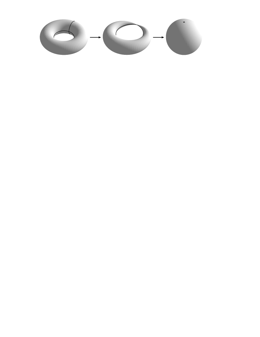
Figure 2: Left: Cartesian product space $S^{1}\times S^{1}$ drawn as a torus, with two circles representing the sets $\{x_{0}\}\times S^{1}$ and $S^{1}\times\{y_{0}\}$ for some arbitrarily chosen points $x_{0}$ and $y_{0}$. Middle: surface after shrinking the first of these sets to a point. Right: surface after shrinking the second set to a point, which gives the smash product $S^{1}\wedge S^{1}\sim S^{2}$.

IV Sphalerons

The word sphaleron is of Greek origin and means “ready to fall” (see Ref. KM84  for the etymology). It is used to denote a static but unstable solution of the classical field equations with finite total energy of the fields.

In this article, only finite-energy configurations of the fields will be considered. By analogy to Morse theory Mil63 , sphalerons can then be looked for by a minimax procedure T82 if the configuration space of the underlying field theory is multiply connected.

The procedure runs as follows: first, construct a noncontractible $p$-dimensional sphere $S^{p}$ in configuration space, then determine its maximal energy configuration, and, finally, “shrink” the sphere to minimize this maximal energy. If the configuration space were compact, this procedure would be guaranteed to give a saddle point. But configuration space is infinite-dimensional and noncompact, so that the minimax procedure produces at best only a candidate solution. It has to be checked explicitly that the appropriate minimax-configuration solves the classical field equations. If this is the case, the minimax-configuration is a genuine sphaleron.

IV.1 Sphaleron $\mathrm{S}$

For the sphaleron $\mathrm{S}\,$ M83 ; KM84 ; DHN74 of the $SU(2)$ Yang–Mills–Higgs theory (1), we consider three-space to be compactified by adding the “sphere at infinity.” Configuration space is then the space of all static three-dimensional gauge and Higgs field configurations in a particular gauge which have finite energy. The static gauge field can be written as a Lie-algebra-valued one-form,

$$A(x^{1},x^{2},x^{3})\equiv A_{m}^{a}(x^{1},x^{2},x^{3})\,\tau^{a}/(2{\rm i})\,{\rm d}x^{m}\,,$$ (3)

with implicit sums of $a$ and $m$ over $1,\,2,\,3$. Furthermore, we use spherical coordinates $(r,\theta,\phi)$ over $\mathbb{R}^{3}$ and employ the radial gauge condition $A_{r}=0$, together with $A_{0}=0$.

Since the energy has to be finite, only those configurations are admissible for which the gauge field tends towards a pure-gauge configuration as $r\to\infty$ and the Higgs field towards its associated vacuum value,

$$g\,A^{\infty}=-{\rm d}\omega\,\omega^{-1}\,,\qquad\Phi^{\infty}=\eta\>\omega\left(\begin{array}[]{c}0\\ 1\end{array}\right)\,,$$ (4)

for a map $\omega$ of the “sphere at infinity” $S^{2}$ into the gauge group $SU(2)$.

Any loop in configuration space induces a loop in the space of these mappings $\omega$. The corresponding map is denoted by

$$U:S^{1}\times S^{2}\to SU(2)\,,\qquad(\mu,\theta,\phi)\mapsto U(\mu,\theta,\phi)\,,$$ (5)

where $\mu\in[0,\pi]$ is the parameter of the loop of configurations and $\theta\in[0,\pi]$ and $\phi\in[0,2\pi]$ are spherical coordinates in three-space.

By imposing certain constraints on this map, we may effectively reduce the set of allowed loops, so that $U$ becomes a map $S^{3}\to SU(2)\sim S^{3}$ which falls into homotopy classes according to $\pi_{3}(SU(2))=\pi_{3}(S^{3})=\mathbb{Z}$. To be specific, the map $U$ for $\mu=0$ and $\mu=\pi$ must not depend on $\theta$ and $\phi$, and the map $U$ for $\theta=0$ has to be independent of $\mu$. Then $U$ is effectively defined on the smash product $S^{1}\wedge S^{2}\sim S^{3}$, as explained in the last paragraph of Section III. Now there exist noncontractible loops of field configurations for which the minimax procedure can be performed.

An appropriate expression for the map (5) is given by M83

$$U(\mu,\theta,\phi)=y^{1}\,(-{\rm i}\tau_{1})+y^{2}\,(-{\rm i}\tau_{2})+y^{3}\,(-{\rm i}\tau_{3})+y^{4}\,\openone_{2}\,,$$ (6)

with

$$\left(\begin{array}[]{c}y^{1}\\ y^{2}\\ y^{3}\\ y^{4}\end{array}\right)=\left(\begin{array}[]{c}-\sin\mu\sin\theta\sin\phi\\ -\sin\mu\sin\theta\cos\phi\\ \sin\mu\cos\mu\,(\cos\theta-1)\\ \cos^{2}\mu+\sin^{2}\mu\cos\theta\end{array}\right)\,.$$ (7)

In order to calculate the winding number of this particular map $U$, we examine its relation to the standard spherical coordinates on $S^{3}$,

$$\left(\begin{array}[]{c}z^{1}\\ z^{2}\\ z^{3}\\ z^{4}\end{array}\right)=\left(\begin{array}[]{l}\cos\theta_{2}\\ \sin\theta_{2}\cos\theta_{1}\\ \sin\theta_{2}\sin\theta_{1}\sin\phi_{1}\\ \sin\theta_{2}\sin\theta_{1}\cos\phi_{1}\end{array}\right)\,,$$ (8)

with polar angles $\theta_{1},\theta_{2}\in[0,\pi]$ and azimuthal angle $\phi_{1}\in[0,2\pi]$.

We first observe that the two-vector

$$\vec{w}=\left(\begin{array}[]{c}\cos\mu\\ \sin\mu\cos\theta\end{array}\right)$$ (9)

sweeps over the unit disk if $\mu$ and $\theta$ run from $0$ to $\pi$. Since rotations map the unit disk onto itself and leave the length of $\vec{w}$ invariant,

$$|\vec{w}|^{2}=1-\sin^{2}\mu\,\sin^{2}\theta\,,$$ (10)

the relation

$$\left(\begin{array}[]{c}\cos\theta_{2}\\ \sin\theta_{2}\cos\theta_{1}\end{array}\right)=\left(\begin{array}[]{cc}\cos\alpha&-\sin\alpha\\ \sin\alpha&\cos\alpha\end{array}\right)\left(\begin{array}[]{c}\cos\mu\\ \sin\mu\cos\theta\end{array}\right)$$ (11)

describes an admissible reparametrization of the disc. By choosing $\alpha=-\mu$, we find $y^{4}=z^{1}$ and $y^{3}=z^{2}$. With $\sin\theta_{1}\sin\theta_{2}=\sin\mu\sin\theta$ and $\phi_{1}=\phi$, we have also $y^{1}=-z^{3}$ and $y^{2}=-z^{4}$.

The conclusion is that the map $U$ as defined by Eqs. (6)–(7) covers the target sphere $S^{3}$ exactly once. The map $U$ has winding number one (or minus one, depending on the definition of the winding number) and corresponds to a nontrivial element of the homotopy group $\pi_{3}(S^{3})=\mathbb{Z}$.

For the static $SU(2)$ gauge and Higgs fields of the noncontractible loop (NCL), we make the Ansatz M83

$$g\,A(\mu,r,\theta,\phi) =-\,f(r)\,\,{\rm d}U(\mu,\theta,\phi)\,\,U(\mu,\theta,\phi)^{-1}\,,$$ (12a)

$$\Phi(\mu,r,\theta,\phi) =\eta\,h(r)\,U(\mu,\theta,\phi)\left(\begin{array}[]{c}0\\ 1\end{array}\right)+\eta\,\Bigl{(}1-h(r)\Bigr{)}\left(\begin{array}[]{c}0\\ \exp(-{\rm i}\,\mu)\cos\mu\end{array}\right),$$ (12f)

with the following boundary conditions for the radial functions $f$ and $h$:

$$\lim_{r\to 0}\,f(r)/r =0\,, \lim_{r\to\infty}\,f(r) =1\,,$$ (13a)

$$\lim_{r\to 0}\,h(r) =0\,, \lim_{r\to\infty}\,h(r) =1\,.$$ (13b)

The energy density of the fields (12) turns out to be spherically symmetric. Indeed, the fields of the NCL can also be written in a manifestly spherically symmetric form K90plb .

The fields (12) of the NCL at $\mu=0$ or $\pi$ correspond to the Higgs vacuum with $A(x)=0$ and $\Phi(x)=(0,\eta)^{\,t}$. This particular configuration is independent of the radial functions $f$ and $h$ and has zero energy according to Eq. (1). The NCL configuration at $\mu=\pi/2$ is distinguished by having parity reflection symmetry (the only other configuration of the NCL with this property is the vacuum at $\mu=0$). For given functions $f$ and $h$, this $\mu=\pi/2$ configuration is also the maximum energy configuration over the NCL. The minimax procedure now consists of adjusting the radial functions $f$ and $h$ while maintaining the boundary conditions (13), so that the energy at $\mu=\pi/2$ is minimized. The resulting configuration is the sphaleron $\mathrm{S}$, as sketched in Fig. 3

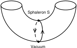
Figure 3: Sphaleron $\mathrm{S}$ on top of a noncontractible loop in configuration space. The field energy is zero for the vacuum and positive for the sphaleron $\mathrm{S}$.

Using numerical methods, one finds for the sphaleron energy the value KM84

$$E_{\mathrm{S}}\approx 3.04\times(4\pi/g^{2})\,M_{W}\,,$$ (14)

which holds for the case of vanishing quartic Higgs coupling constant ($\lambda/g^{2}=0$). [The sphaleron energy $E_{\mathrm{S}}$ has also been calculated for the full $SU(2)\times U(1)$ Yang–Mills–Higgs theory of the electroweak Standard Model. The energy $E_{\mathrm{S}}$ is found to be weakly dependent on the mixing angle $\theta_{w}$, at least near $\theta_{w}=0$. The emergence of a large magnetic dipole moment $\mu_{\mathrm{S}}\propto(4\pi/g^{2})\,g\,\tan\theta_{w}/M_{W}$ is perhaps more interesting. See Refs. KM84 ; KKB92 ; HJ94 for details.] For large enough values of $\lambda/g^{2}$, additional solutions appear, the so-called “deformed sphalerons” KB89 ; Y89 . The appearance of these extra sphalerons can be explained K90plb by a simple deformation of the energy surface in Fig. 3.

The sphaleron $\mathrm{S}\,$ by itself has trivial topology, with the “sphere at infinity” $S^{2}$ mapped into the Higgs vacuum manifold $SU(2)\sim S^{3}$; cf. Section III. (As mentioned in the Introduction, the magnetic monopole tHP74 in $SU(2)$ Yang–Mills theory with a real isotriplet of Higgs is based on the nontrivial map $S^{2}\to SO(3)/SO(2)\sim S^{2}$.) Note that the original $\mathrm{S}\,$ Ansatz, with the so-called hedgehog structure, was discovered DHN74 ten years before the construction of $\mathrm{S}\,$ via the NCL M83 ; KM84 .

In the radial gauge, the vacuum configuration of the $SU(2)$ gauge field is uniquely fixed, $gA_{m}^{\rm vac}(x^{1},x^{2},x^{3})=0$. If this gauge condition is abandoned, any pure-gauge configuration $gA_{m}=-\partial_{m}U\,U^{-1}$, for arbitrary time-independent $SU(2)$-valued field $U$, is a possible vacuum configuration. Depending on the topology of three-space, these vacuum configurations may or may not fall into different unconnected classes. This does not happen for our compactification $\mathbb{R}^{3}\cup S^{2}_{\infty}$. But the situation changes if, instead, we choose a one-point compactification $\mathbb{R}^{3}\cup\{\infty\}$, with all fields approaching a single direction-independent value as $r\to\infty$. Each vacuum configuration then corresponds to a map $S^{3}\to S^{3}$ and there are topologically distinct vacuum classes, since $\pi_{3}(S^{3})=\mathbb{Z}$.

In fact, it is possible to perform a gauge transformation on the NCL (12) which changes the asymptotic behavior of the gauge fields, so that they can be considered to live on $S^{3}=\mathbb{R}^{3}\cup\{\infty\}$. Let $\omega(\mu,r,\theta,\phi)$ be an $SU(2)$-valued map which approaches $U(\mu,\theta,\phi)$ for $r\to\infty$ and $\openone_{2}$ for $r\to 0$. The radial dependence of $\omega(\mu,r,\theta,\phi)$ implements a path which connects the map $U(\mu,\theta,\phi)=\omega(\mu,\infty,\theta,\phi)$ to the constant map $\openone_{2}=\omega(\mu,0,\theta,\phi)$. [Note that $U(\mu,\theta,\phi)$ for fixed $\mu$ is a map $S^{2}\to S^{3}$ and therefore contractible.]

The crucial point, now, is that the map $\omega(0,r,\theta,\phi)$ is homotopically different from the map $\omega(\pi,r,\theta,\phi)$. [Otherwise, the radial dependence of $\omega(\mu,r,\theta,\phi)$ would yield a contraction of $\omega(\mu,\infty,\theta,\phi)$, considered as a $\mu$-dependent map $S^{3}\to S^{3}$, which is impossible.] Both maps $\omega(0,r,\theta,\phi)$ and $\omega(\pi,r,\theta,\phi)$ can also be viewed as maps $S^{3}\to S^{3}$, since $\omega(\mu,\infty,\theta,\phi)=U(\mu,\theta,\phi)=\openone_{2}$ for $\mu=0$ and $\mu=\pi$. The conclusion is then that the corresponding vacuum configurations $A_{m}(x^{1},x^{2},x^{3})$ at $\mu=0$ and $\mu=\pi$ belong to different homotopy classes. This result will be discussed further in Section VI.1.

IV.2 Sphaleron $\mathrm{S}^{*}$

The three-space of our $SU(2)$ Yang–Mills–Higgs theory (1) is again compactified by adding the “sphere at infinity.” This time, however, we do not consider one-parameter families (loops) of static finite-energy configurations but two-parameter families (spheres). At spatial infinity, these families are characterized by the map

$$U:S^{2}\times S^{2}\to SU(2)\,,\qquad(\mu,\nu,\theta,\phi)\mapsto U(\mu,\nu,\theta,\phi)\,,$$ (15)

where ($\mu$, $\nu$) are the parameters of the sphere of configurations and ($\theta$, $\phi$) are the polar and azimuthal angles of the spherical coordinates in three-space. The parameters $\mu$ and $\nu$ run from $-\pi/2$ to $+\pi/2$ and the boundary of the ($\mu$,$\nu$)-square at $|\mu|=\pi/2$ or $|\nu|=\pi/2$ is mapped to the same element of $SU(2)$.

Next, restrict the class of mappings $U$ by requiring that $U(\mu,\nu,0,\phi)$ is independent of $(\mu$, $\nu$, $\phi)$ and $U(-\pi/2,-\pi/2,\theta,\phi)$ independent of $(\theta$, $\phi)$. Then $U$ is effectively a mapping from $S^{4}$ to $S^{3}$, which has a nontrivial homotopy structure, $\pi_{4}(S^{3})=\mathbb{Z}_{2}$. The general idea, now, is to construct a noncontractible sphere, to determine the maximal energy configuration on that sphere and to continuously deform the sphere so that its maximal energy is minimized K85 .

The construction of the required nontrivial map $S^{4}\to S^{3}$ is done in two steps. First, a nontrivial map $S^{3}\to S^{2}$ is found and, second, an operation is performed to increase the dimension of both spheres.

The relevant map $S^{3}\to S^{2}$ is given by the well-known Hopf fibration Nak90 , which can be explained as follows. Consider the three-sphere $S^{3}$ to be a subset of $\mathbb{C}^{2}$, namely $\{(z_{1},z_{2})\,|\;|z_{1}|^{2}+|z_{2}|^{2}=1\}$. Each $\mathbb{C}$-line through the origin in $\mathbb{C}^{2}$ then intersects with this three-sphere in a great circle $S^{1}$. These great circles $S^{1}$ form a pairwise disjoint covering of $S^{3}$. Two points of $S^{3}$ are defined to be equivalent ($\simeq$), if they lie on the same great circle $S^{1}$. The corresponding projection,

$$S^{3}\to S^{3}/\simeq\,,$$ (16)

is the desired Hopf map, since the topological space $S^{3}/\simeq\>$ is homeomorphic to $S^{2}$.

The topological equivalence of $S^{3}/\simeq\>$ and $S^{2}$ can be shown by considering the $\mathbb{C}$-lines which label the great circles $S^{1}$ discussed in the previous paragraph. All but one of these $\mathbb{C}$-lines can be parametrized by complex numbers $c\in\mathbb{C}$. Specifically, the coordinates of such a line read

$$\left(z_{1}\,,\,z_{2}\right)=(w\,,\,c\>w)\,,\qquad\mathrm{for}\;\;w\in\mathbb{C}\,.$$ (17)

In addition, there is the single $\mathbb{C}$-line given by

$$\left(z_{1}\,,\,z_{2}\right)=(0\,,\,w)\,,\qquad\mathrm{for}\;\;w\in\mathbb{C}\,.$$ (18)

Hence, the total parameter space of $S^{3}/\simeq$ is given by the one-point-compactified plane, i.e., the Riemann sphere $S^{2}$.

The suspension of a sphere $S^{n}$ is essentially the same as the smash product $S^{1}\wedge S^{n}$. It can be used to increase the dimension of the spheres appearing in the above discussion. The resulting suspension of the Hopf map corresponds to a nontrivial element of the homotopy group $\pi_{4}(S^{3})=\mathbb{Z}_{2}$.

In a particular parametrization, the required map (15) takes the form K85

$$U(\mu,\nu,\hat{x}) = \bigl{(}\,\sin\mu+{\rm i}\cos\mu\,\,\exp[\,+{\rm i}(\nu+\pi/2)\,\tau_{3}\,]\,\,\hat{x}\cdot\vec{\tau}\,\,\exp[\,-{\rm i}(\nu+\pi/2)\,\tau_{3}\,]\,\bigr{)}$$ (19)

$$\times\bigl{(}\,\sin\mu-{\rm i}\cos\mu\,\,\hat{x}\cdot\vec{\tau}\,\bigr{)}\,,$$

where $\mu$ and $\nu$ range over $[-\pi/2,\pi/2]$ and describe a two-sphere, as does the unit three-vector $\hat{x}\equiv(\sin\theta\cos\phi,\sin\theta\sin\phi,\cos\theta)$. The map $U(\mu,\nu,\hat{x})$ is effectively defined on the smash product $S^{2}\wedge S^{2}$, since $U$ is independent of $\hat{x}$ for $\mu=\pm\pi/2$ or $\nu=\pm\pi/2$ and independent of $\mu$ and $\nu$ for $\hat{x}=(0,0,1)$. (Note that the suspended Hopf map also plays a role in the physics of Skyrme solitons WZ83 .)

With the map (19) in hand, it is possible to construct a noncontractible sphere (NCS) of static Yang–Mills–Higgs configurations and to obtain the corresponding nontrivial classical solution, the sphaleron $\mathrm{S}^{*}$, just as for the NCL and the sphaleron $\mathrm{S}$ of the previous subsection. The construction of $\mathrm{S}^{*}$ is, however, rather subtle. Here, we only describe the four basic steps and refer the reader to Ref. K93 for more information.

First, we observe that the map (19) singles out the $x^{3}$ axis, which suggests the use of the cylindrical coordinates $\rho$, $\phi$, and $z$, defined by $(x^{1},x^{2},x^{3})=(\rho\cos\phi,\rho\sin\phi,z)$. Then, it is not difficult to construct a NCS of static $SU(2)$ Yang–Mills–Higgs configurations, whose behavior at infinity is governed by the $SU(2)$ matrix (19). Specifically, the NCS configurations can be written in terms of six axial functions $f_{i}(\rho,z)$ and $h_{j}(\rho,z)$, for $i=0,1,2,3$ and $j=1,2$, with appropriate boundary conditions (for example, $f_{0}(\rho,z)\to 1$ and $h_{1}(\rho,z)\to 1$ as $\rho^{2}+z^{2}\to\infty$). The $SU(2)$ gauge and Higgs field configuration of the NCS are by construction axially symmetric.

Second, the configuration at $\mu=\nu=0$ is also invariant under parity reflection and gives the maximum energy of the NCS. Moreover, it can be verified that this $\mu=\nu=0$ configuration, in terms of the six axial functions $f_{i}(\rho,z)$ and $h_{j}(\rho,z)$, provides a self-consistent Ansatz for the $SU(2)$ Yang–Mills–Higgs field equations. Concretely, this means that the Ansatz reduces the field equations to precisely six partial differential equations (PDEs) for the six functions $f_{i}(\rho,z)$ and $h_{j}(\rho,z)$, with appropriate boundary conditions which trace back in part to the finite-energy condition. (This result agrees with the so-called principle of symmetric criticality P79 , which states that, under certain conditions, it suffices to consider variations that respect the symmetry of the Ansatz.) The solution of these PDEs then determines the field configurations of the sphaleron $\mathrm{S}^{*}$. See Fig. 4 for a sketch of configuration space.

Figure 4: Sphaleron $\mathrm{S}^{*}$ on top of a noncontractible sphere in configuration space.

Third, the reduced field equations for the sphaleron $\mathrm{S}^{*}$ can be solved numerically. For approximately vanishing quartic Higgs coupling constant ($\lambda/g^{2}=1/800$), the numerical solution of the six PDEs with the correct boundary conditions gives the following value for the energy:

$$E_{\mathrm{S}^{*}}\approx 1.91\times E_{\mathrm{S}}\,,$$ (20)

where $E_{\mathrm{S}}$ denotes the corresponding energy of the sphaleron $\mathrm{S}$ [cf. Eq. (14) above]. In fact, the sphaleron $\mathrm{S}^{*}$ is found to have the structure of a di-atomic molecule, binding together a sphaleron $\mathrm{S}$ and an “anti-sphaleron” $\bar{\mathrm{S}}$. See Ref. K93 for a plot of the energy density and further discussion.

Fourth, the construction of $\mathrm{S}^{*}$ via the NCS can be extended to the full $SU(2)\times U(1)$ theory of the electroweak Standard Model by the introduction of one more axial function, $f_{4}(\rho,z)$, with trivial boundary conditions at infinity. But for nonvanishing weak mixing angle $\theta_{w}$, there are only preliminary numerical results for the sphaleron $\mathrm{S}^{*}$ and it would be worthwhile to obtain accurate results over the full range of values of $\lambda/g^{2}$ and $\theta_{w}$.

IV.3 $Z$-string

Now consider static field configurations of the $SU(2)$ Yang–Mills–Higgs theory (1) which are independent of one spatial coordinate, the $z$-coordinate, and have vanishing gauge potential in that direction, $A_{z}=0$. In order to have finite total energy, the $z$-direction has to be compact and three-space is taken to be $\mathbb{R}^{2}\times S^{1}$ instead of $\mathbb{R}^{3}$. Also, choose cylindrical polar coordinates ($\rho$, $\phi$, $z$) and work in the polar gauge for which $A_{\rho}=0$.

Since the energy density in a plane with fixed $z$ has to be finite, the remaining gauge field component $A_{\phi}$ reduces to a pure-gauge configuration asymptotically,

$$g\,A_{\phi}\to-\,(\partial_{\phi}\,\omega)\,\,\omega^{-1}\,,\quad\mathrm{as}\;\;\rho\to\infty\,,$$ (21)

for a map $\omega:S^{1}\to SU(2)$. Basically, this means that the plane $\mathbb{R}^{2}$ is compactified by adding the “circle at infinity.”

It is possible to construct a noncontractible sphere of these field configurations by restricting the corresponding maps

$$U:S^{2}\times S^{1}\to SU(2)\,,\qquad(\mu,\nu,\phi)\mapsto U(\mu,\nu,\phi)\,,$$ (22)

in such a way that they are effectively defined on the smash product $S^{2}\wedge S^{1}\sim S^{3}$. Specifically, the sphere is parametrized by $\mu$ and $\nu$ which take values in $[-\pi/2,+\pi/2]$. The rim of the ($\mu$,$\nu$)-square is identified and corresponds to a single point on $S^{2}$. The map $U$ is restricted to be independent of $\phi$ if $(\mu,\nu)$ lies on this rim and independent of ($\mu$,$\nu$) if $\phi=0$.

An appropriate expression for the map (22) is given by KO94

$$U(\mu,\nu,\phi) =V(\mu,\nu,0)^{-1}\,V(\mu,\nu,\phi)\,,$$ (23a)

$$V(\mu,\nu,\phi) =z^{1}\,(-{\rm i}\tau_{1})+z^{2}\,(-{\rm i}\tau_{2})+z^{3}\,(-{\rm i}\tau_{3})+z^{4}\,\openone_{2}\,,$$ (23b)

$$\left(\begin{array}[]{c}z^{1}\\ z^{2}\\ z^{3}\\ z^{4}\end{array}\right) =\left(\begin{array}[]{l}\sin\mu\\ \cos\mu\sin\nu\\ \cos\mu\cos\nu\sin\phi\\ \cos\mu\cos\nu\cos\phi\end{array}\right)\,.$$ (23k)

Note that the factor $V(\mu,\nu,0)^{-1}$ in (23a) serves a dual purpose. First, it assures that the rim of the ($\mu$,$\nu$)-square is mapped to a single element, since $V(\mu,\nu,\phi)$ is independent of $\phi$ on this boundary. Second, it makes $U$ independent of $\mu$ and $\nu$ if $\phi=0$.

For the two-dimensional $SU(2)$ gauge and Higgs fields of the noncontractible sphere (NCS), we make the Ansatz KO94

$$g\,A(\mu,\nu,\rho,\phi) =-f(\rho)\>{\rm d}U(\mu,\nu,\phi)\,U(\mu,\nu,\phi)^{-1}\,,$$ (24a)

$$\Phi(\mu,\nu,\rho,\phi) =\eta\,h(\rho)\,U(\mu,\nu,\phi)\left(\begin{array}[]{c}0\\ 1\end{array}\right)\,,$$ (24d)

with parameters $|\mu|,|\nu|\leq\pi/2$. The polar functions $f$ and $h$ have the following boundary conditions:

$$\lim_{\rho\to 0}\,f(\rho)/\rho =0\,, \lim_{\rho\to\infty}\,f(\rho) =1\,,$$ (25a)

$$\lim_{\rho\to 0}\,h(\rho) =0\,, \lim_{\rho\to\infty}\,h(\rho) =1\,.$$ (25b)

But no point on this NCS corresponds to a vacuum configuration, since the Higgs field in Eq. (24d) vanishes at $\rho=0$ for all values of $(\mu,\nu)$. Therefore, the point of the NCS at the boundary of the ($\mu$,$\nu$)-square must be connected to the vacuum by an additional line segment. The corresponding Ansatz is simply

$$g\,A(\mu,\nu,\rho,\phi) =0\,,$$ (26a)

$$\Phi(\mu,\nu,\rho,\phi) =\eta\,\Bigl{(}1-\sin[\mu\nu]+h(\rho)\,\sin[\mu\nu]\,\Bigr{)}\,\left(\begin{array}[]{c}0\\ 1\end{array}\right)\,,$$ (26d)

for $[\mu\nu]\equiv\max\{|\mu|,|\nu|\}>\pi/2$ with the parameter range of $\mu$ and $\nu$ extended to $[-\pi,+\pi]$. The set of configurations (23)–(26) is like a “balloon” which is tied to the ground by a rope.

Figure 5: $Z$-string on top of a noncontractible sphere (balloon) in configuration space.

The energy of the NCS has a global maximum at $\mu=\nu=0$. By minimizing this maximal energy with respect to the functions $f$ and $h$, one finds the coupled differential equations

$$\rho\,f^{\prime\prime}-f^{\prime} ={\textstyle\frac{1}{2}}\,g^{2}\eta^{2}\,\rho\,h^{2}\,(f-1)\,,$$ (27a)

$$\rho^{2}\,h^{\prime\prime}+\rho\,h^{\prime} =h\,(1-f)^{2}+2\lambda\eta^{2}\,\rho^{2}h\,(h^{2}-1)\,,$$ (27b)

where the prime indicates a derivative with respect to $\rho$. The same differential equations, with boundary conditions (25), hold for the so-called $Z$-string NO73 ; N77 ; JPV93 , which excites the $Z\,$ boson and Higgs fields of the electroweak Standard Model.

The $Z$-string is thus the sphaleron on the NCS given by Eqs. (23)–(26); see Fig. 5. This particular sphere (balloon) in configuration space will be discussed further in Section VI.3. Note, finally, that the configurations of the NCS can also be embedded in the full $SU(2)\times U(1)$ gauge theory of the electroweak Standard Model; see Ref. KO94 for details and numerical results.

V Spectral flow

The classical field configurations of the previous section may serve as background fields for massless Dirac fermions, whose left-handed components form an isodoublet under the $SU(2)$ gauge group and whose right-handed components are gauge singlets. The Dirac equation for the spinor $\Psi(x)$ reads in this case

$$\left({\rm i}D\!\!\!\!/\,-k\,(\Phi_{M}^{\dagger}P_{L}+\Phi_{M}P_{R})\right)\Psi=0\,,$$ (28)

with the Yukawa coupling constant $k$, the Feynman slash notation $D\!\!\!\!/\,\equiv\gamma^{\mu}D_{\mu}$, and the covariant derivative

$$D_{\mu}\Psi(x)\equiv\left[\,\partial_{\mu}+gA_{\mu}(x)P_{L}\,\right]\Psi(x)\,,$$ (29)

which shows that only the left-handed fermions interact with the $SU(2)$ gauge field.

The left- and right-handed projectors are, as usual, defined by $P_{L}\equiv{\textstyle\frac{1}{2}}(\openone-\gamma_{5})$ and $P_{R}\equiv{\textstyle\frac{1}{2}}(\openone+\gamma_{5})$. With the Minkowski metric of Section II, the Dirac matrices obey the following Clifford algebra and Hermiticity conditions:

$$\gamma^{\mu}\gamma^{\nu}+\gamma^{\nu}\gamma^{\mu}=2\,g^{\mu\nu}\,,\;\;\;\gamma^{\mu\,\dagger}=\gamma^{0}\gamma^{\mu}\gamma^{0}\,,\;\;\;\gamma_{5}\equiv{\rm i}\,\gamma^{0}\gamma^{1}\gamma^{2}\gamma^{3}=\gamma_{5}^{\dagger}\,.$$ (30)

(For the Euclidean metric, all Dirac matrices are chosen Hermitian, $\gamma^{\mu\,\dagger}=\gamma^{\mu}$.) The spacetime manifold considered in this article is flat and there is no need to use the vierbeins (tetrads) explicitly.

The matrix $\Phi_{M}$ in (28) contains the two Higgs field components $\Phi_{1}$ and $\Phi_{2}$,

$$\Phi_{M}=\left(\begin{array}[]{cc}\Phi_{2}^{*}&\Phi_{1}\\ -\Phi_{1}^{*}&\Phi_{2}\end{array}\right)\,,$$ (31)

so that

$$\Phi_{M}\cdot\left(\begin{array}[]{c}0\\ 1\end{array}\right)=\left(\begin{array}[]{c}\Phi_{1}\\ \Phi_{2}\end{array}\right)=\Phi\,.$$ (32)

For the Higgs vacuum with $A_{\mu}(x)=0$ and $\Phi_{M}(x)=\mathrm{diag}(\eta,\eta)$, the effective fermion mass is given by $m=k\,\eta$.

The model considered may serve as the starting point for a consistently renormalized quantum field theory with gauge group $SU(2)\times U(1)$ if we include three colors of left-handed quark isodoublets for each left-handed lepton isodoublet, so that the perturbative gauge anomalies A69 ; BJ69 ; AB69 ; B69 cancel between the quarks and the leptons BIM72 ; GJ72 . (A similar cancellation occurs for the nonperturbative $SU(2)$ anomaly W82 to be discussed in Section VI.2.) But, for our purpose, it suffices to consider a single isodoublet of left-handed fermions, since the fermion isodoublets of the full theory behave identically.

The time-dependent solutions of the Dirac equation (28) are, however, not our main interest. Rather, we are interested in the eigenvalues $E$ of the corresponding Dirac Hamiltonian,

$$H=-{\rm i}\gamma^{0}\gamma^{m}D_{m}+k\,\gamma^{0}\left(\,\Phi_{M}^{\dagger}P_{L}+\Phi_{M}P_{R}\,\right)\,,$$ (33)

where use has been made of the fact that $A_{0}=0$ for our gauge field configurations and the covariant derivative $D_{m}$, for $m=1,2,3$, has already been given in Eq. (29). The eigenvalues $E$ are real, since the Dirac Hamiltonian $H$ is Hermitian.

Now consider periodic one-parameter families (loops) of static background fields. The spectral flow invariant APS75 is then defined as the number of eigenvalues that cross zero from below minus the number of eigenvalues that cross zero from above as the loop parameter varies over its range (in a prescribed direction). See, e.g., Ref. A85 for an elementary introduction to the concept of spectral flow.

Even if the spectral flow invariant vanishes, there may still be a nontrivial rearrangement (permutation) of the energy levels. We speak about “spectral flow” also in this case. (Mathematicians would perhaps say that there is no spectral flow if the spectral flow invariant is zero.) In addition, we will look for “spectral flow” in two-parameter families of background fields (which may be characterized by a different topological invariant).

V.1 Spectral flow for the sphaleron $\mathrm{S}$

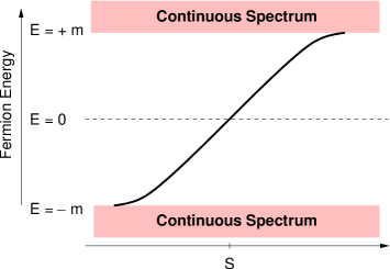
Figure 6: Spectral flow for a path over the sphaleron barrier (cf. Fig. 3).

Consider the noncontractible loop (NCL) used in Section IV.1 to construct the sphaleron $\mathrm{S}$, with parameter $\mu$ running from $0$ to $\pi$. At the beginning of the loop ($\mu=0$) and at the end ($\mu=\pi$), the static background field (12) is the same vacuum configuration and the spectrum of the Dirac Hamiltonian (33) is purely continuous with a mass gap $2m$ according to the Higgs mechanism ($m\propto\eta$). For the sphaleron $\mathrm{S}$ at $\mu=\pi/2$, on the other hand, it has been shown N75 ; JR76 ; KM84aps ; R88 ; KB93 that the Dirac Hamiltonian $H$ has a single normalizable eigenfunction with eigenvalue zero.

The overall picture, starting from $\mu=0$, is that a negative eigenvalue $E(\mu)$ of the Dirac Hamiltonian $H$ rises above the negative continuous spectrum, crosses zero when the background fields pass the sphaleron barrier ($\mu=\pi/2$), and finally reaches the positive continuous spectrum for $\mu=\pi$. See Fig. 6 for a sketch and Ref. KB93 for numerical results.

The nonvanishing spectral flow over the NCL is guaranteed by the Atiyah–Singer index theorem AS68 , which relates the analytic index of the four-dimensional Dirac operator (the loop parameter $\mu$ playing the role of an imaginary time) to the topological charge associated with the NCL. Further details will be given in Section VI.1. Here, we only remark that the NCL gauge field (12), defined in Minkowski space, has essentially the same topology as the BPST instanton solution of Euclidean Yang–Mills theory BPST75 ; BC78 .

V.2 Spectral flow for the sphaleron $\mathrm{S}^{*}$

For the fermion behavior over the noncontractible sphere (NCS) through $\mathrm{S}^{*}$, we need to resort to more abstract reasoning, since no complete numerical or analytic solution has been obtained up till now.

First, consider massless Dirac fermions with equal gauge couplings for the right- and left-handed components. It has then been shown that there exist two fermion zero-modes of the four-dimensional Euclidean Dirac operator ${\rm i}D\!\!\!\!/\,_{4}$, one of each chirality, if the fermions are placed in the background of the constrained instanton $\mathrm{I}^{*}$ K93npb ; KW96 ; K98npb . (Note that a particular time slice through $\mathrm{I}^{*}$ corresponds to the three-dimensional configuration of the $\mathrm{S}^{*}$ sphaleron. For practical purposes, one may consider $\mathrm{I}^{*}$ as a bound state of a BPST instanton $\mathrm{I}$ and an anti-instanton $\bar{\mathrm{I}}$, just as the sphaleron $\mathrm{S}^{*}$ may be viewed as a composite of a sphaleron $\mathrm{S}$ and an anti-sphaleron $\bar{\mathrm{S}}$; see Eq. (20) and the lines below.)

Now the instanton $\mathrm{I}^{*}$, which depends on four Euclidean spacetime coordinates, can be viewed as a path in configuration space which passes over the $\mathrm{S}^{*}$ barrier. (In other words, this path is homotopic to a particular closed loop on the $\mathrm{S}^{*}$-NCS modulo gauge transformations; cf. Fig. 4.) The two zero-modes of ${\rm i}D\!\!\!\!/\,_{4}$ in the $\mathrm{I}^{*}$ background, being time-dependent solutions of the Dirac equation (with imaginary time), can be calculated in the adiabatic approximation, where the state at time $t$ is an eigenstate of the Dirac Hamiltonian with energy $E(t)$. The corresponding “phase factor” is given by

$$\exp\left(-\int_{0}^{t}\!{\rm d}t^{\prime}\,E(t^{\prime})\right)\,.$$ (34)

From the normalizability of the zero-mode, it follows that $E(t)$ is positive for $t\to+\infty$ and negative for $t\to-\infty$.

With left- and right-handed chiralities, there are then two energy levels $E^{(1,2)}(t)$ crossing zero from below (these energy levels may, of course, be degenerate). In addition, there are two eigenvalues $E^{(3,4)}(t)$ which cross zero from above, so that the total spectral flow invariant is zero (note that the loop through $\mathrm{S}^{*}$ over the NCS is contractible). For these last two eigenvalues, there are no zero-modes of ${\rm i}D\!\!\!\!/\,_{4}$ because the corresponding four-dimensional wave functions are not normalizable. Thus we have two pairs of levels which cross at zero energy, one left-handed pair and one right-handed pair. Returning to the Dirac Hamiltonian (33) with only left-handed fermions interacting with the $SU(2)$ gauge fields, we have the spectral flow of the eigenvalues $E^{(1)}(t)$ and $E^{(3)}(t)$ as shown in Fig. 7.

Figure 7: Spectral flow for a path through the sphaleron $\mathrm{S}^{*}$ (cf. Fig. 4).

Recently, numerical results B03 have been obtained for the eigenvalues of the ${\rm i}D\!\!\!\!/\,_{4}$ operator along a particular path over the $\mathrm{I}^{*}$ barrier. It would be interesting to use similar methods to calculate the spectral flow related to $\mathrm{S}^{*}$ and also to consider fermion representations other than isodoublet.

V.3 Spectral flow for the $Z$-string

Finally, we turn to the fermion behavior over the noncontractible sphere (NCS) with the $Z$-string at the top KR97 . First, we choose a path on the NCS (23)–(26), which starts in the vacuum, passes over the $Z$-string and ends up in the vacuum.

To be concrete, we put $\nu=0$ in (23) and let $\mu$ run from $-\pi/2$ to $+\pi/2$. Such a loop is contractible and there is no net spectral flow to be expected (just as for the loop through $\mathrm{S}^{*}$ considered in the previous subsection). What happens instead is that one negative eigenvalue $E^{(1)}(\mu,0)$ is raised from the negative continuous spectrum and one positive eigenvalue $E^{(2)}(\mu,0)$ is lowered from the positive continuous spectrum. Both eigenvalues meet at energy zero when the background fields pass the $Z$-string configuration ($\mu=\nu=0$), cross and reach the opposite region of continuous eigenvalues (see the picture on the left in Fig. 8). The fermion zero-modes of the $Z$-string have been studied in Refs. JR81 ; EP94 .

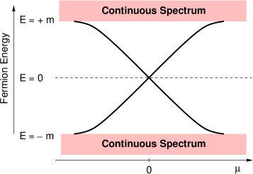
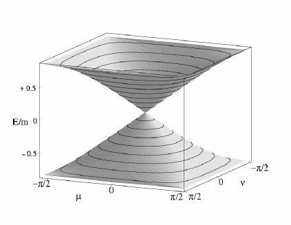
Figure 8: Spectral flow over the noncontractible sphere (NCS) through the $Z$-string (cf. Fig. 5). In the picture on the left, the NCS parameter $\nu$ is held fixed at the value $0$ and $\mu$ is varied. In the picture on the right, the Dirac eigenvalues are shown for the NCS patch $|\mu|,|\nu|\leq\pi/2$.

We can also consider the behavior of the Dirac eigenvalues over the whole two-parameter family (24). Plotted over the ($\mu$,$\nu$)-square, the eigenvalues $E(\mu,\nu)$ form a double cone meeting at $\mu=\nu=0$ (see the picture on the right in Fig. 8).

VI Anomalies

In this section, we review the relation between the sphalerons presented in Section IV and so-called anomalies. The connection between sphalerons and anomalies is precisely the spectral flow discussed in Section V.

VI.1 Chiral anomaly and fermion number violation

The chiral $U(1)$ anomaly, which turns out to be related to the sphaleron $\mathrm{S}$, eliminates a rigid $U(1)$ symmetry of the classical action, viz. chiral invariance. This anomaly can be found in theories with massless fermions, for which there is a classical Ward identity

$$\sum_{f}\left(\,\frac{\delta\Gamma_{\rm cl}}{\delta\Psi_{f}}\;\delta\Psi_{f}-\delta\bar{\Psi}_{f}\;\frac{\delta\Gamma_{\rm cl}}{\delta\bar{\Psi}_{f}}\,\right)=\partial^{\mu}j_{\mu}^{5}\,,$$ (35)

where $\Gamma_{\rm cl}$ is the classical action and $\Psi_{f}(x)$ denotes a Dirac fermion field, with $f$ labeling the different flavors (fermion species). The rigid chiral transformation of the fermion fields is given by

$$\delta\Psi_{f}(x)={\rm i}\gamma_{5}\,\Psi_{f}(x)\,,\qquad\delta\bar{\Psi}_{f}(x)=\bar{\Psi}_{f}(x)\,{\rm i}\gamma_{5}\,.$$ (36)

Since the left-hand side of (35) vanishes for solutions of the classical equations of motion, the current $j_{\mu}^{5}(x)\equiv\sum_{f}\bar{\Psi}_{f}(x)\,\gamma_{5}\gamma_{\mu}\Psi_{f}(x)$ is conserved classically. This implies that the chiral charge $Q_{5}\equiv\int{\rm d}^{3}x\,j_{0}^{5}(x)$ does not change with time ($t\equiv x^{0}$),

$$\left.\frac{\mathrm{d}Q_{5}}{\mathrm{d}t}\right|_{\mathrm{\,classical}}=0\,.$$ (37)

Now suppose that the $SU(2)$ gauge field couples equally to left- and right-handed fermions in the fundamental representation (as is the case for the $SU(3)$ gauge field which is believed to be responsible for quark confinement in the Standard Model). Then the spectral flow for a path over the sphaleron $\mathrm{S}$ with unit winding number is as shown in Fig. 9: for each isodoublet of fermions a left-handed state crosses zero from below and a right-handed one crosses zero from above. (Essentially the same type of spectral flow has been found M85 in the Schwinger model, i.e., two-dimensional quantum electrodynamics with a massless Dirac fermion.) In the Dirac-sea picture of the second-quantized vacuum, this means that a pair of fermions is created from an initial vacuum state, namely one chiral fermion and one chiral antiparticle corresponding to a hole in the Dirac sea of antichiral negative-energy states. Hence, the total chiral charge $Q_{5}$ changes by two units per isodoublet, which contradicts the classical conservation equation (37).

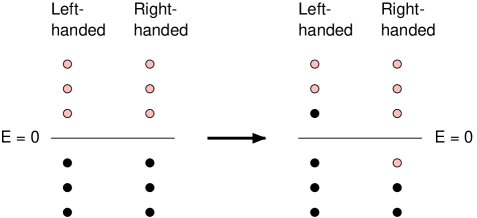
Figure 9: Opposite spectral flow for left- and right-handed fermions, which leads to the creation of two units of chiral charge. Filled states are drawn black, empty states gray.

This result is supported by the Atiyah–Singer index theorem AS68 for the four-dimensional chiral Dirac operator (see, e.g., Refs. JR77 ; F80 ; B00 ). For $N$ isodoublets, the relation between the change of chiral charge and the appropriate characteristic of the background gauge field is simply the integrated version of the perturbative Ward identity for the chiral current containing the Adler–Bell–Jackiw anomaly A69 ; BJ69 ,

$$\sum_{f=1}^{N}\left(\,\frac{\delta\Gamma}{\delta\Psi_{f}}\;\delta\Psi_{f}-\delta\bar{\Psi}_{f}\;\frac{\delta\Gamma}{\delta\bar{\Psi}_{f}}\,\right)=\left[\,\partial^{\mu}j_{\mu}^{5}\,\right]\bullet\Gamma\,+\,\frac{g^{2}\,N}{8\,\pi^{2}}\,\,\left[\text{tr}\,\,\tilde{F}_{\mu\nu}\,F^{\mu\nu}\right]\bullet\Gamma\,,$$ (38)

where $\Gamma$ is now the fully quantized vertex functional and the bullet denotes an operator insertion.

The anomalous term in Eq. (38) includes the Pontryagin density

$$q(x)\equiv-\,\frac{g^{2}}{16\,\pi^{2}}\,\text{tr}\,\,\tilde{F}_{\mu\nu}(x)\,F^{\mu\nu}(x)\,,$$ (39)

with $\tilde{F}_{\mu\nu}\equiv(1/2)\,\epsilon_{\mu\nu\rho\sigma}F^{\rho\sigma}$. The integral of this density over the spacetime manifold $M$ is a topological invariant called the Pontryagin index,

$$Q\equiv\int_{M}{\rm d}^{4}x\;q(x)\,.$$ (40)

For compact spacetime manifolds $M$, the Pontryagin index is an integer number and is also called the winding number or topological “charge” (hence, the notation $Q$).

Next, turn to the simplified version of the electroweak Standard Model, as described in Sections II and V. Here, the fermion fields are fundamentally massless, even though they behave as massive particles in the Higgs vacuum. More importantly, the gauge field now couples only to the left-handed parts of the fermion fields; cf. Eqs. (28) and (29). Hence, the spectral flow for a single fermion flavor is made up of only one state which crosses zero from below. This implies that fermion number conservation is violated tH76prl ; tH76prd . See Fig. 10 and compare with Fig. 9. (It is, of course, important to define carefully what is meant by “the fermion number” of a given state C80 ; GH95 ; Kh95 ; see also the discussion in the last three paragraphs of this subsection.)

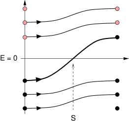
Figure 10: Spectral flow in the electroweak Standard Model, where only left-handed fermions interact with the $SU(2)$ gauge fields. $\mathrm{S}\,$ denotes the sphaleron, which has a single fermion zero-mode. The spectral flow leads to a change of fermion number between initial and final states (see text).

The map $U$ given in Section IV.1 essentially provides a map $S^{3}\to S^{3}$, characterized by the topological charge $|Q|=1$. The above considerations can be generalized to other (integer) values of $Q$ and to a model with $N_{\rm fam}$ families of quarks and leptons. The sum of baryon number $B$ and lepton number $L$ is then found to be nonconserved tH76prl ,

$$\Delta(B-L)=0\,,\quad\Delta(B+L)=2\,N_{\rm fam}\,Q\,,$$ (41)

where $\Delta B$ denotes the change of baryon number between initial and final states and similarly for $\Delta L$.

As explained at the end of Section IV.1, the NCL can be transformed into a path connecting two topologically distinct vacua in one-point-compactified three-space. The general form of such a vacuum is given by a static pure-gauge configuration,

$$g\,A=-{\rm d}\chi\,\chi^{-1}\,,\qquad\Phi=\eta\,\chi\left(\begin{array}[]{c}0\\ 1\end{array}\right)\,,$$ (42)

for a map $\chi:\mathbb{R}^{3}\to SU(2)$ which approaches $\openone_{2}$ at spatial infinity. The homotopy class to which $\chi$ belongs is characterized by the integer Chern–Simons number

$$N_{\mathrm{CS}}[\,\chi\,]=-\,\frac{1}{24\,\pi^{2}}\int{\rm d}^{3}x\>\epsilon^{klm}\,\,\text{tr}\left\{(\partial_{k}\chi\,\chi^{-1})\,(\partial_{l}\chi\,\chi^{-1})\,(\partial_{m}\chi\,\chi^{-1})\right\}\,.$$ (43)

The topological charge $Q$ of the map $\omega(\mu,r,\theta,\phi)$, as discussed in the last two paragraphs of Section IV.1, is then the difference of the Chern–Simons numbers of the vacua at the start and end of the associated path,

$$Q=\Delta N_{\mathrm{CS}}\equiv N_{\mathrm{CS}}[\,\omega(\pi,r,\theta,\phi)\,]-N_{\mathrm{CS}}[\,\omega(0,r,\theta,\phi)\,]\,.$$ (44)

Of course, it is also possible to map the $\mu$-interval $[0,\pi]$ on the time interval $[-\infty,+\infty]$.

The sphaleron now corresponds to an energy barrier between these vacua, as sketched in Fig. 11. The transition between different vacua can, for example, take place by tunneling through the sphaleron barrier tH76prl ; tH76prd or by passing over the barrier due to a thermal fluctuation of the fields KM84 ; DS78 . Especially the latter mechanism is expected to contribute significantly to fermion-number-violating processes in the early universe (see, e.g., Refs. McL94 ; RS96 ).

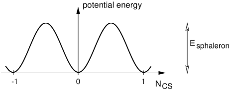
Figure 11: Potential energy over a slice of configuration space, parametrized by the Chern–Simons number $N_{\mathrm{CS}}$. The height of the energy barrier between topologically different vacua ($N_{\mathrm{CS}}=n\in\mathbb{Z}$) is set by the sphaleron S, which appears in different gauge copies ($N_{\mathrm{CS}}=1/2+n$, for $n\in\mathbb{Z}$). This figure essentially “unwraps” the loop of Fig. 3.

The rate of fermion-number-violating processes at relatively low energies ($E\ll E_{\mathrm{S}}\approx 10\;\mathrm{TeV}$) can be calculated from the Euclidean path integral tH76prd ; R90 . But for a reliable discussion of these processes at high energies ($E\gtrsim E_{\mathrm{S}}$) it is advisable to remain in Minkowski spacetime. The problem, then, is that the compactification of four-space which we used as the starting point of our topological considerations is not really physically sensible for Minkowski spacetime. The topological charge $Q$, in particular, need not be an integer quantity in Minkowski spacetime. The crucial point here is the role of energy conservation for background fields that solve the equations of motion; see, e.g., Ref. FKS93 . The general question of which type of gauge field leads to nontrivial spectral flow remains unanswered for the moment.

There exists, however, a result for strongly dissipative $SU(2)$ gauge fields C80 ; GH95 ; Kh95 . In this case, the spectral flow is given by the difference in winding numbers of the asymptotic vacuum configurations for $t\to\pm\infty$. Roughly speaking, this coincides with the previous result in Euclidean spacetime, namely Eq. (44) inserted into Eq. (41).

For the case of spherically symmetric fields, there is also a result for generic (i.e., nondissipative) gauge fields,

$$\Delta(B-L)=0\,,\quad\Delta(B+L)=2\,N_{\rm fam}\,\left(\Delta N_{\mathrm{winding}}+\Delta N_{\rm twist}\right)\,\Bigr{|}_{\mathrm{spher.\;symm.}}\,.$$ (45)

The change of $B+L$ is now determined by two integers. The first, $\Delta N_{\mathrm{winding}}$, again corresponds to Eq. (44). But the second, $\Delta N_{\rm twist}$, is an entirely new characteristic of spherically symmetric $SU(2)$ gauge fields, which is related to the asymptotic behavior of the solutions of a (nonlinear) Riccati equation embedded in the (linear) zero-energy Dirac equation KL01 . The integer $\Delta N_{\rm twist}$ is zero for strongly dissipative $SU(2)$ gauge fields. See Ref. K02blois for further discussion of the issues involved.

VI.2 Witten’s global gauge anomaly

The global $SU(2)$ gauge anomaly, which turns out to be related to the sphaleron $\mathrm{S}^{*}$, differs from the case discussed in the previous subsection in that not just a symmetry of the theory is eliminated but the theory itself.

As mentioned in Section V.2, the crossing of energy levels for paths over the $\mathrm{S}^{*}$ barrier is related to the existence of two normalizable zero-modes of the four-dimensional Euclidean Dirac operator ${\rm i}D\!\!\!\!/\,_{4}$, one of each chirality. The noncontractible sphere of three-dimensional configurations can also be viewed as a noncontractible loop of four-dimensional configurations. Furthermore, as explained at the end of Section IV.1, it is possible to pass from a loop of gauge field configurations in the radial gauge to a path of gauge field configurations without the radial gauge condition. The resulting path has topologically inequivalent vacua at the start and at the end.

Now consider the change of eigenvalues of ${\rm i}D\!\!\!\!/\,_{4}$ along such a path. Since for one “point” of the path (i.e., the $\mathrm{I}^{*}$-configuration) there are known zero-modes K98npb , it is to be expected that some level crossing is occurring also here.

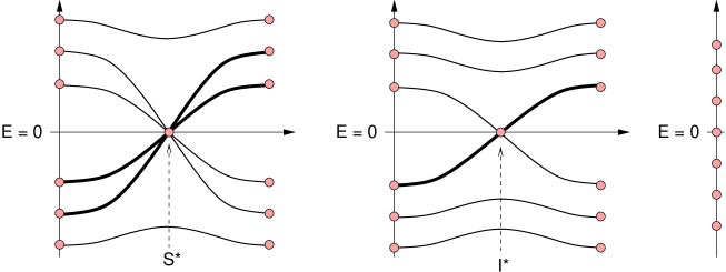
Figure 12: Left: sketch of the eigenvalues of the Dirac Hamiltonian for a particular path over the $\mathrm{S}^{*}$ noncontractible sphere (the theory considered has both left- and right-handed fermions interacting with the $SU(2)$ gauge fields, which is not the case in Fig. 7). Middle: eigenvalues of ${\rm i}D\!\!\!\!/\,_{4}$ for the corresponding noncontractible loop through the constrained instanton $\mathrm{I}^{*}$. Right: eigenvalues of ${\rm i}D\!\!\!\!/\,_{5}$ for the corresponding five-dimensional configuration. Each path with an energy level crossing zero from below (thick line) corresponds to a normalizable fermion zero-mode one dimension higher. The sphaleron $\mathrm{S}^{*}$ has four fermion zero-modes, the constrained instanton $\mathrm{I}^{*}$ two, and the five-dimensional configuration one.

That this is indeed the case has been shown in Ref. W82 by increasing the dimension once more. The one-parameter family of four-dimensional Dirac operators can also be considered as a single five-dimensional one. (In other words, the whole NCS serves as a single background configuration.) It then follows from the so-called mod–2 Atiyah–Singer index theorem AS71 that the corresponding five-dimensional Dirac operator has a normalizable zero-mode. For ${\rm i}D\!\!\!\!/\,_{4}$, this implies that an eigenvalue is crossing zero from negative to positive values as the path is traversed. Simultaneously, there is a second eigenvalue which passes from positive to negative values. This discussion is summarized in Fig. 12, which also gives the corresponding spectral flow in three dimensions. (The mod–2 index theorem guarantees only an odd number of zero-modes for the five-dimensional configuration, but for simplicity we have assumed there is just one. See Ref. B03 for numerical results and further discussion.)

Witten also argued that the spectral flow of ${\rm i}D\!\!\!\!/\,_{4}$ leads to a global gauge anomaly W82 . In the Euclidean path integral of $SU(2)$ Yang–Mills theory with a single isodoublet of Weyl fermions, there effectively appears a square root of the Dirac determinant,

$$\int{\mathcal{D}}A_{\mu}\;\;\sqrt{\det{\rm i}D\!\!\!\!/\,_{4}}\;\;\exp\left(\,\frac{1}{2}\int\!\!{\rm d}^{4}x\,\,\text{tr}\,F_{\mu\nu}F^{\mu\nu}\,\right)\,,$$ (46)

if one recalls that two Weyl fermions of opposite chiralities make a single Dirac fermion.

The Dirac determinant in Eq. (46) depends on the background gauge fields $A_{\mu}(x)$ and its square root can be defined as the product of the positive eigenvalues [ starting from a given gauge field configuration, say $A_{\mu}(x)=0\,$]. The above considerations then show that for a particular continuous variation of the gauge fields we end up with gauge fields, which are related to the starting configuration by a large gauge transformation and which have a $\sqrt{\det{\rm i}D\!\!\!\!/\,_{4}}$ of opposite sign (one positive eigenvalue having become negative; cf. the middle picture of Fig. 12). In the path integral, one has to integrate over all gauge fields (taking out the infinite factor due to gauge invariance afterwards). Hence, for every contribution $\sqrt{\det{\rm i}D\!\!\!\!/\,_{4}}$ there is also a contribution $-\sqrt{\det{\rm i}D\!\!\!\!/\,_{4}}$ arising from the gauge-transformed background fields. This implies that the path integral (46) vanishes.

More precisely, the path integral over the gauge fields is not well defined, because there is no satisfactory way to restrict the integration over the gauge fields so that a single Weyl isodoublet gives a continuous gauge-invariant contribution. This, then, is the Witten anomaly, which can also be proven without the mod–2 Atiyah–Singer index theorem but with the perturbative Bardeen anomaly instead EN84 ; K91plb .

VI.3 $Z$-string global gauge anomaly

Just as for the Witten anomaly and the $\mathrm{S}^{*}$ sphaleron of the previous subsection, there exists a global gauge anomaly related to the $Z$-string sphaleron KR97 . In order to explain this anomaly, we need a modified noncontractible sphere (NCS), obtained by continuous deformation of the balloon as given in Section IV.3. This modification has the advantage of being a real sphere, that is, without degenerate points. The modified NCS still has one point corresponding to the vacuum and one point corresponding to the $Z$-string (see the picture in the middle of Fig. 13).

For the modified NCS, the $z$-independent $SU(2)$ gauge field is in the polar gauge $A_{\rho}=0$. But like the case of the sphalerons $\mathrm{S}$ and $\mathrm{S}^{*}$, it is possible to relax the polar gauge condition and to demand instead that the vacuum reached for $\rho\to\infty$ is the trivial one. Then one ends up with a disc of configurations with a loop of pure-gauge configurations on the boundary (see the picture on the right of Fig. 13). Considering the compactified radial coordinate $\rho$ to be a polar angle $\theta$, the fields are effectively defined on a sphere $S^{2}$. The loop of vacuum configurations on this two-sphere, restricted to the smash product $S^{1}\wedge S^{2}$, corresponds to a nontrivial element of the homotopy group $\pi_{3}(S^{3})$.

Figure 13: $Z$-balloon, $Z$-sphere and $Z$-disc.

We keep this in mind for later and turn to the eigenvalues of the four-dimensional Euclidean Dirac operator ${\rm i}D\!\!\!\!/\,_{4}$, where the time-dependent background fields are taken to be paths over the $Z$-disc, with the start and end point (not necessarily the same) lying on the rim of vacuum configurations. For any such path passing through the $Z$-string, we know from Section V.3 that ${\rm i}D\!\!\!\!/\,_{4}$ has a single normalizable zero-mode corresponding to the eigenvalue of the Dirac Hamiltonian which crosses zero from below.

Now consider a particular family of operators ${\rm i}D\!\!\!\!/\,_{4}$ corresponding to a family of paths over the $Z$-disc, which starts from a constant path corresponding to a point on the rim of the disc, passes through a path via the $Z$-string, and ends up in a pure vacuum path formed by the boundary of the disc (see Fig. 14, where the $Z$-disc of Fig. 13 has been flattened). This family of four-dimensional Dirac operators sweeps over the whole $Z$-disc and we expect that there is spectral flow corresponding to the winding number of the underlying map $S^{3}\to S^{3}$. In our case, this means that a single eigenvalue of ${\rm i}D\!\!\!\!/\,_{4}$ crosses zero. The zero crossing can be expected to occur for the path labeled $(3)$ in Fig. 14.

Figure 14: Five closed loops on the $Z$-disc (cf. Fig. 13). Loop (1) corresponds to a single point on the boundary, loop (3) passes through the $Z$-string, and loop (5) consists of the whole boundary of the disc.

Like the case of the Witten anomaly in Section VI.2, this prevents us from defining the square root of the fermion determinant as a continuous gauge-invariant function of the bosonic background fields. Note that our path of four-dimensional configurations begins in a time-independent, topologically trivial vacuum and ends up in a gauge-transformed, time-dependent and topologically nontrivial one.

It is particularly interesting to see how this global gauge anomaly manifests itself in the space of time-independent fermion states. Since the Dirac Hamiltonian is a real Hermitian operator, we may choose real energy-eigenstates. Concretely, look at the one-dimensional subspace spanned by the eigenstate which crosses zero from below in the picture on the left in Fig. 8. For the background fields, we use an arbitrary loop on the $Z$-disc, which circumnavigates the $Z$-string exactly once and which is parametrized by $\alpha\in[0,2\pi]$. Then the energy eigenstate defines a real line bundle over $S^{1}$.

It has been shown in Ref. KR97 that this bundle is, in fact, the Möbius bundle. A normalized eigenstate $|\Phi(0)\rangle$ transported around the loop ends up as $|\Phi(2\pi)\rangle=-|\Phi(0)\rangle$; see Fig. 15. The phase factor found is determined by the Berry phase for adiabatic transport B84 . The Berry phase $\pi\pmod{2\pi}$ is of topological origin and does not change under continuous deformation of the loop, as long as the loop of configurations does not touch the fermion degeneracy “point” corresponding to the $Z$-string. This observation also shows that the boundary of the $Z$-disc (Fig. 13) is a noncontractible loop of vacuum configurations, since the real Berry phase factor $-1$ on it cannot be continuously changed to $+1$.

The variation of the eigenstate along the rim of the $Z$-disc defines a projective action of the gauge group on the fermionic matter. There is then a global gauge anomaly, because it is impossible to define a real, continuous, and proper (i.e., nonprojective) representation of the local gauge group on the fermion states. Since the vacuum of quantum field theory is the Dirac sea with all negative-energy eigenstates filled, this also means that the second-quantized vacuum state acquires the Berry phase factor $-1$. See Section 6 of Ref. KR97 for further discussion. (We take the opportunity to correct a slip of the pen. In the last sentence of Footnote 6 in Ref. KR97 , the words “and vice versa” must be deleted.)

A similar interpretation of the Witten anomaly in terms of a Berry phase has been given in Ref. NA85 . There is, however, a crucial difference between the $Z$-string global gauge anomaly and the Witten anomaly. For the $Z$-string anomaly, namely, there does exist a local counterterm in the action which restores gauge invariance, but at the price of violating Lorentz and CPT invariance K98npb2 . More generally, if gauge invariance is enforced, there appears a new anomaly, the so-called CPT anomaly (see Refs. K00npb ; KS02 for the main result and Ref. K01wigner for a review).

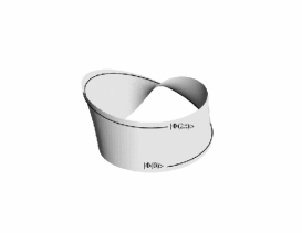
Figure 15: Möbius bundle structure of the gauge orbit, with loop parameter $\alpha\in[0,2\pi]$. The line represents a normalized real eigenstate $|\Phi(\alpha)\rangle$ of the Dirac Hamiltonian, with $|\Phi(2\pi)\rangle=-|\Phi(0)\rangle$.

VII Conclusion

The space of finite-energy three-dimensional field configurations of $SU(2)$ Yang–Mills–Higgs theory (in short, configuration space) has nontrivial topology T82 ; M83 , which leads to the existence of a new type of classical solutions, the so-called sphalerons. Sphalerons are unstable static finite-energy solutions of the classical field equations, whereas solitons are stable solutions.

In Section IV, we have explained the topology behind the $\mathrm{S}$, $\mathrm{S}^{*}$, and $Z$-string sphalerons KM84 ; K93 ; KO94 of the $SU(2)$ Yang–Mills–Higgs theory (1). Precisely this theory appears in the electroweak Standard Model of elementary particle interactions EWSM . Knowledge of these classical solutions may, therefore, be of great importance to physics.

Adding chiral fermions to the $SU(2)$ Yang–Mills–Higgs theory, the nontrivial topology of configuration space makes itself felt by the occurrence of spectral flow APS75 , as discussed in Section V. In turn, the general phenomenon of spectral flow is related to the possible existence of anomalies which invalidate certain properties of the classical theory, as discussed in Section VI.

The spectral flow over a noncontractible loop through the sphaleron $\mathrm{S}$ is related to the chiral $U(1)$ anomaly A69 ; BJ69 , which corresponds to a breakdown of baryon and lepton number conservation in the electroweak Standard Model tH76prl . The spectral flow through the $\mathrm{S}^{*}$ and $Z$-string sphalerons does not lead to a global $SU(2)$ gauge anomaly W82 ; KR97 , because the electroweak Standard Model has an even number of chiral isodoublets. Still, there is nontrivial spectral flow (more precisely, spectral rearrangement) over configuration space, but its physical implications remain to be clarified (cf. Refs. K98npb ; K00npb ). Indeed, we need a better understanding of the role of configuration space topology in concrete physical problems, such as the behavior of elementary particle fields at high energies or temperatures.

References

-
(1)
T.H.R. Skyrme, “A non-linear field theory,”
Proc. R. Soc. London Ser. A 260 (1960) 127;
T.H.R. Skyrme, “A unified field theory of mesons and baryons,” Nucl. Phys. 31 (1962) 556. -
(2)
G. ’t Hooft,
“Magnetic monopoles in unified gauge theories,”
Nucl. Phys. B 79 (1974) 276;
A.M. Polyakov, “Particle spectrum in quantum field theory,” JETP Lett. 20 (1974) 194 [Pisma Zh. Eksp. Teor. Fiz. 20 (1974) 430]. -
(3)
C.H. Taubes,
“The existence of a non-minimal solution to the
Yang–Mills–Higgs equations on ,”
Commun. Math. Phys. 86 (1982) 257; 86 (1982) 299;
C.H. Taubes, “Min-max theory for the Yang–Mills–Higgs equations,” Commun. Math. Phys. 97 (1985) 473. - (4) N.S. Manton, “Topology in the Weinberg–Salam theory,” Phys. Rev. D 28 (1983) 2019.
- (5) F.R. Klinkhamer and N.S. Manton, “A saddle point solution in the Weinberg–Salam theory,” Phys. Rev. D 30 (1984) 2212.
- (6) F.R. Klinkhamer, “Construction of a new electroweak sphaleron,” Nucl. Phys. B 410 (1993) 343 [arXiv:hep-ph/9306295].
- (7) F.R. Klinkhamer and P. Olesen, “A new perspective on electroweak strings,” Nucl. Phys. B 422 (1994) 227 [arXiv:hep-ph/9402207].
-
(8)
S.L. Glashow,
“Partial symmetries of weak interactions,”
Nucl. Phys. 22 (1961) 579;
S. Weinberg, “A model of leptons,” Phys. Rev. Lett. 19 (1967) 1264;
A. Salam, “Weak and electromagnetic interactions,” in: Elementary Particle Theory, edited by N. Svartholm (Almqvist, Stockholm, 1968), p. 367;
S.L. Glashow, J. Iliopoulos and L. Maiani, “Weak interactions with lepton–hadron symmetry,” Phys. Rev. D 2 (1970) 1285. - (9) L.D. McLerran, “B+L nonconservation as a semiclassical process,” Acta Phys. Polon. B 25 (1994) 309 [arXiv:hep-ph/9311239].
- (10) V.A. Rubakov and M.E. Shaposhnikov, “Electroweak baryon number non-conservation in the early universe and in high-energy collisions,” Usp. Fiz. Nauk 166 (1996) 493 [Phys. Usp. 39 (1996) 461] [arXiv:hep-ph/9603208].
- (11) M. Nakahara, Geometry, Topology and Physics, Institute of Physics Publishing, Bristol, 1990.
- (12) J. Milnor, Morse Theory, Princeton University Press, Princeton, 1963.
- (13) R. Dashen, B. Hasslacher and A. Neveu, “Nonperturbative methods and extended hadron models in field theory. III. Four-dimensional nonabelian models,” Phys. Rev. D 10 (1974) 4138.
- (14) F.R. Klinkhamer, “Sphalerons, deformed sphalerons and configuration space,” Phys. Lett. 236 B (1990) 187.
- (15) J. Kunz, B. Kleihaus and Y.Brihaye, “Sphalerons at finite mixing angle,” Phys. Rev. D 46 (1992) 3587.
- (16) M. Hindmarsh and M. James, “The origin of the sphaleron dipole moment,” Phys. Rev. D 49 (1994) 6109 [arXiv:hep-ph/9307205].
- (17) J. Kunz and Y. Brihaye, “New sphalerons in the Weinberg-Salam theory,” Phys. Lett. B 216 (1989) 353.
- (18) L.G. Yaffe, “Static solutions of Higgs theory,” Phys. Rev. D 40 (1989) 3463.
- (19) F.R. Klinkhamer, “A new sphaleron in the Weinberg-Salam theory?,” Z. Phys. C 29 (1985) 153.
- (20) F. Wilczek and A. Zee, “Linking numbers, spin, and statistics of solitons,” Phys. Rev. Lett. 51 (1983) 2250.
- (21) R.S. Palais, “The principle of symmetric criticality,” Commun. Math. Phys. 69 (1979) 19.
- (22) H.B. Nielsen and P. Olesen, “Vortex-line models for dual strings,” Nucl. Phys. B 61 (1973) 45.
- (23) Y. Nambu, “String-like configurations in the Weinberg–Salam theory,” Nucl. Phys. B 130 (1977) 505.
- (24) M. James, L. Perivolaropoulos and T. Vachaspati, “Detailed stability analysis of electroweak strings,” Nucl. Phys. B 395 (1993) 534 [arXiv:hep-ph/9212301].
- (25) S.L. Adler, “Axial vector vertex in spinor electrodynamics,” Phys. Rev. 177 (1969) 2426.
- (26) J.S. Bell and R. Jackiw, “A PCAC puzzle: in the sigma model,” Nuovo Cimento A 60 (1969) 47.
- (27) S.L. Adler and W.A. Bardeen, “Absence of higher order corrections in the anomalous axial vector divergence equation,” Phys. Rev. 182 (1969) 1517.
- (28) W.A. Bardeen, “Anomalous Ward identities in spinor field theories,” Phys. Rev. 184 (1969) 1848.
- (29) C. Bouchiat, J. Iliopoulos and P. Meyer, “An anomaly free version of Weinberg’s model,” Phys. Lett. B 38 (1972) 519.
- (30) D.J. Gross and R. Jackiw, “Effect of anomalies on quasirenormalizable theories,” Phys. Rev. D 6 (1972) 477.
- (31) E. Witten, “An ) anomaly,” Phys. Lett. B 117 (1982) 324.
- (32) M. Atiyah, V.K. Patodi and I.M. Singer, “Spectral asymmetry and Riemannian geometry”, Math. Proc. Camb. Phil. Soc. 77 (1975) 43; 78 (1975) 405; 79 (1976) 71.
- (33) M. Atiyah, “Topological aspects of anomalies,” in: Symposium on Anomalies, Geometry, Topology, edited by W.A. Bardeen and A.R. White, World Scientific, Singapore, 1985, p. 22.
- (34) C.R. Nohl, “Bound state solutions of the Dirac equation in extended hadron models,” Phys. Rev. D 12 (1975) 1840.
- (35) R. Jackiw and C. Rebbi, “Solitons with fermion number 1/2,” Phys. Rev. D 13 (1976) 3398.
- (36) F.R. Klinkhamer and N.S. Manton, “A saddle-point solution in the Weinberg–Salam theory,” in: Proceedings of the 1984 Summer Study on the Design and Utilization of the Superconducting Super Collider, edited by R. Donaldson and J. Morfin (American Physical Society, New York, 1984), p. 805.
- (37) A. Ringwald, “Sphaleron and level crossing,” Phys. Lett. B 213 (1988) 61.
- (38) J. Kunz and Y. Brihaye, “Fermions in the background of the sphaleron barrier,” Phys. Lett. B 304 (1993) 141 [arXiv:hep-ph/9302313].
- (39) M. Atiyah and I.M. Singer, “The index of elliptic operators I, III, IV”, Ann. Math. 87 (1968) 484; 87 (1968) 546; 93 (1971) 119.
- (40) A.A. Belavin, A.M. Polyakov, A.S. Schwartz and Y.S. Tyupkin, “Pseudoparticle solutions of the Yang-Mills equations,” Phys. Lett. B 59 (1975) 85.
- (41) K.M. Bitar and S.J. Chang, “Vacuum tunneling of gauge theory in Minkowski space,” Phys. Rev. D 17 (1978) 486.
- (42) F.R. Klinkhamer, “Existence of a new instanton in constrained Yang–Mills–Higgs theory,” Nucl. Phys. B 407 (1993) 88 [arXiv:hep-ph/9306208].
- (43) F.R. Klinkhamer and J. Weller, “Construction of a new constrained instanton in Yang–Mills–Higgs theory,” Nucl. Phys. B 481 (1996) 403 [arXiv:hep-ph/9606481].
- (44) F.R. Klinkhamer, “Fermion zero-modes of a new constrained instanton in Yang–Mills–Higgs theory,” Nucl. Phys. B 517 (1998) 142 [arXiv:hep-th/9709194].
- (45) O. Bär, “On Witten’s global anomaly for higher representations,” Nucl. Phys. B 650 (2003) 522 [arXiv:hep-lat/0209098].
- (46) F.R. Klinkhamer and C. Rupp, “A global anomaly from the -string,” Nucl. Phys. B 495 (1997) 172 [arXiv:hep-th/9702023].
- (47) R. Jackiw and P. Rossi, “Zero modes of the vortex–fermion system,” Nucl. Phys. B 190 (1981) 681.
- (48) M.A. Earnshaw and W.B. Perkins, “Stability of an electroweak string with a fermion condensate,” Phys. Lett. B 328 (1994) 337 [arXiv:hep-ph/9402218].
- (49) N.S. Manton, “The Schwinger model and its axial anomaly,” Ann. Phys. (N.Y.) 159 (1985) 220.
- (50) R. Jackiw and C. Rebbi, “Spinor analysis of Yang–Mills theory,” Phys. Rev. D 16 (1977) 1052.
- (51) K. Fujikawa, “Path integral for gauge theories with fermions,” Phys. Rev. D 21 (1980) 2848; Erratum 22 (1980) 1499.
- (52) R.A. Bertlmann, Anomalies in Quantum Field Theory, Oxford University Press, Oxford, 2000.
- (53) G. ’t Hooft, “Symmetry breaking through Bell–Jackiw anomalies,” Phys. Rev. Lett. 37 (1976) 8.
- (54) G. ’t Hooft, “Computation of the quantum effects due to a four-dimensional pseudoparticle,” Phys. Rev. D 14 (1976) 3432; Erratum 18 (1978) 2199.
- (55) N.H. Christ, “Conservation law violation at high-energy by anomalies,” Phys. Rev. D 21 (1980) 1591.
- (56) T.M. Gould and S.D. Hsu, “Anomalous violation of conservation laws in Minkowski space,” Nucl. Phys. B 446 (1995) 35 [arXiv:hep-ph/9410407].
- (57) V.V. Khoze, “Fermion number violation in the background of a gauge field in Minkowski space,” Nucl. Phys. B 445 (1995) 270 [arXiv:hep-ph/9502342].
- (58) S. Dimopoulos and L. Susskind, “Baryon number of the universe,” Phys. Rev. D 18 (1978) 4500.
-
(59)
A. Ringwald,
“High-energy breakdown of perturbation theory in the electroweak
instanton sector,” Nucl. Phys. B 330 (1990) 1;
O. Espinosa, “High-energy behavior of baryon and lepton number violating scattering amplitudes and breakdown of unitarity in the Standard Model,” Nucl. Phys. B 343 (1990) 310;
S.Y. Khlebnikov, V.A. Rubakov and P.G. Tinyakov, “Instanton induced cross-sections below the Sphaleron,” Nucl. Phys. B 350 (1991) 441. - (60) E. Farhi, V.V. Khoze, and R. Singleton, “Minkowski space nonabelian classical solutions with noninteger winding number change,” Phys. Rev. D 47 (1993) 5551.
- (61) F.R. Klinkhamer and Y.J. Lee, “Spectral flow of chiral fermions in nondissipative gauge field backgrounds,” Phys. Rev. D 64 (2001) 065024 [arXiv:hep-th/0104096].
- (62) F.R. Klinkhamer, “Electroweak baryon number violation,” in: XIV-th Rencontre de Blois: Matter–Antimatter Asymmetry, edited by L. Iconomidou-Fayard and J. Tran Thanh Van, in press [arXiv:hep-ph/0209227].
- (63) M.F. Atiyah and I.M. Singer, “The index of elliptic operators V,” Ann. Math. 93 (1971) 139.
- (64) S. Elitzur and V.P. Nair, “Nonperturbative anomalies in higher dimensions,” Nucl. Phys. B 243 (1984) 205.
- (65) F.R. Klinkhamer, “Another look at the anomaly,” Phys. Lett. B 256 (1991) 41.
- (66) M.V. Berry, “Quantal phase factors accompanying adiabatic changes,” Proc. R. Soc. London Ser. A 392 (1984) 45.
- (67) P. Nelson and L. Alvarez-Gaumé, “Hamiltonian interpretation of anomalies,” Commun. Math. Phys. 99 (1985) 103.
- (68) F.R. Klinkhamer, “-string global gauge anomaly and Lorentz non-invariance,” Nucl. Phys. B 535 (1998) 233 [arXiv:hep-th/9805095].
- (69) F.R. Klinkhamer, “A CPT anomaly,” Nucl. Phys. B 578 (2000) 277 [arXiv:hep-th/9912169].
- (70) F.R. Klinkhamer and J. Schimmel, “CPT anomaly: a rigorous result in four dimensions,” Nucl. Phys. B 639 (2002) 241 [arXiv:hep-th/0205038].
- (71) F.R. Klinkhamer, “CPT violation: mechanism and phenomenology,” in: Proceedings of the Seventh International Wigner Symposium, edited by M.E. Noz, in press [arXiv:hep-th/0110135].