Evidence that highly non-uniform black strings have a conical waist

Abstract

Numerical methods have allowed the construction of vacuum non-uniform strings. For sufficient non-uniformity, the local geometry about the minimal horizon sphere (the “waist”) was conjectured to be a cone metric. We are able to test this conjecture explicitly giving strong evidence in favour of it. We also show how to extend the conjecture to weakly charged strings.

hep-th/0304070

I Introduction and Summary

In the presence of compact dimensions massive solutions of vacuum General Relativity may take one of several forms including the black-hole and the black-string. For concreteness, consider the simplest case - $d-1$ extended space-time dimensions and a compact dimension of radius $L$, which is denoted here by the $z$ coordinate. Any $d\geq 5$ may be considered, and here we specialise to $d=6$ for numerical convenience. The transition between the black hole and string phases, which can be defined by their distinct horizon topologies, must depend on the sole dimensionless parameter of the problem, namely the ratio of the typical curvature radius of the horizon and $L$. The picture we advocate here is that black objects with curvature radius much smaller than $L$ are expected to closely resemble a 6d Schwarzschild black hole, with a nearly round ${\bf S}^{4}$ horizon, while very massive black objects will have a horizon size much larger than $L$ and will be extended over the $z$ axis wrapping it completely. Such objects will have ${\bf S}^{3}\times{\bf S}^{1}$ horizon topology and will be referred to as “black strings”. The simplest black string is a product of the 5d Schwarzschild solution with the spectator $z$ coordinate line and we refer to it as the “uniform string”. Other string solutions which are $z$ dependent we refer to as “non-uniform”. Gregory and Laflamme (GL) Gregory and Laflamme (1993, 1988) discovered that neutral uniform black strings develop a perturbative $z$-dependent instability (tachyon) for masses below a critical mass $m(L)$. Consequently the marginally tachyonic mode generates a branch of static solutions which we call the “GL non-uniform strings”. Interesting links to thermodynamic stability were explored in Gubser and Mitra (2000, 2001); Reall (2001); Gregory and Ross (2001), and the instability was further studied in Chamblin et al. (2000); Gregory (2000); Hirayama and Kang (2001); Gibbons and Hartnoll (2002).

One of the authors (BK) Kol (2002a) used qualitative tools to analyse the phase structure of the static solutions. The emerging picture consists of exactly two stable phases – the black hole and the (stable) uniform black string connected through the unstable GL non-uniform solutions in a first order phase transition. These two stable solutions have not only different horizon topologies, but the total topology of the Euclidean solutions is different as well. Thus a continuous topology change (much like the conifold transition in Calabi-Yau 3-folds) occurs, which was argued to centre around the cone over ${\bf S}^{2}\times{\bf S}^{d-3}$.

This conjecture addresses two questions. Firstly it conjectures that there is only one solution for large mass objects. This question is clearly essential for understanding how astrophysical black holes are manifested, and whether there are potentially observable consequences. Secondly, based on Gubser’s higher order perturbative construction of the GL non-uniform strings Gubser (2002), it predicts all strings in this branch have higher mass than the unstable uniform strings, and so these solutions are unlikely to be the end state for GL decay as suggested by Horowitz and Maeda Horowitz and Maeda (2001). For another approach to the phase structure see Harmark and Obers (2002). For implications to black hole uniqueness and for a description of the explosive transitions with Planck-scale power see Kol (2002b, c).

Let us recall the reason for the appearance of the cone and some more details. One considers a highly non-uniform string as well as a large black hole (a black hole which hardly fits in the compact dimension) and focuses on the vicinity of the “waist” – the minimal sphere in the black string, and on the “gap” between “north” and “south” poles in the black hole. Then one finds that the topology at some distance away from the waist is ${\bf S}^{2}\times{\bf S}^{d-3}$ where the second sphere comes simply from the spherical symmetry and the first includes the Euclidean time. Moreover the spatial ${\bf S}^{d-3}$ is topologically trivial in the black hole (it can shrink) and correspondingly the ${\bf S}^{2}$ for the black string. Hence a topology change analogous to the “pyramid picture” of the conifold suggests itself where the cone here is over the metrically round ${\bf S}^{2}\times{\bf S}^{d-3}$. The isometry of the cone is enhanced (relative to the rest of the solution) and in particular the geometry near the waist depends on only one variable – the distance $\rho$ from the waist. Not only does this enhanced symmetry realize the topology change in a simple setting, but the equations of motion actually forbid some more general ansatze which were tried.

Analytic solutions are not available, despite some attempts Smet (2002); Harmark and Obers (2002) and some relevant constructions in 4-d Myers (1987); Korotkin and Nicolai (1994); Frolov and Frolov (2003) (where the proper size of the compact dimension does not asymptote to a constant, and there are no black string solutions), which do not generalise to $d>4$ Emparan and Reall (2002). One of the authors (TW) Wiseman (2002, 2003a) showed that in general the numerical method of relaxation could be applied to gravitostatics by overcoming the conceptual issues (largely related to imposing the constraint equations and boundary conditions) and in particular was able to trace numerically the GL branch of non-uniform strings in the case $d=6$. Large amounts of non-uniformity were reached ($R_{\mbox{max}}/R_{\mbox{min}}\sim 9$) exposing the asymptotic behaviour for the GL non-uniform branch including limiting mass and temperature. Moreover, it was found that the whole branch has a mass higher than the critical string and therefore cannot serve as an endpoint for decay of unstable uniform strings. The agreement with the theoretical predictions of Kol (2002a) were further strengthened in Wiseman (2003b) where global properties of the solutions were studied and shown to behave in accord with the conjecture.

In this paper we perform a much stronger test of the conjecture in Kol (2002a) by comparing the numerical geometries with the predicted cone. A summary of the method and results follows.

First one is required to identify the transformation from cone coordinates to the numerical metric, and then to compare the two metrics. The cleanest coordinate to extract is $\rho$, and the “smoking gun” test involves comparing the numerical Kretschmann curvature invariant $K_{num}$ with the cone prediction, $K_{cone}$, which due to the symmetry properties of the cone, only depends on $\rho$. A quantitative test shows that over a region where $K$ changes by orders of magnitude agreement is found and $K_{num}/K_{cone}$ changes only by a factor of about two, which we consider to be a sub-leading effect . Next we infer the azimuthal angle $\chi$ from the numerical solution. Actually, comparison of the metric gives $\sin(\chi)$ and so we must test that the maximum of the expression for $\sin(\chi)$ is consistent with 1, and we see this is the case. Three metric functions remain to be compared, and indeed show good agreement. This agreement is particularly satisfying given the low resolution of the grid over the relevant region, and the finite value of non-uniformity which can be achieved.

In summary, we conclude that the numerical 6-d geometry at the vicinity of the waist reveals what is essentially a cone structure, supporting the analysis of Kol (2002a). Sub-leading deviations from the cone remain and may hold further clues and refinements. We conclude with an argument that the waist cone geometry remains a good approximation if the string carries a small electric charge, and construct the behaviour of the electric potential near the cone tip.

II Numerical string solutions

Following Gubser, we define,

$$\lambda=\frac{1}{2}\left(\frac{R_{max}}{R_{min}}-1\right)$$ (1)

where $R_{max,min}$ are the maximum and minimum sphere radii in the horizon. Non-uniform strings were constructed non-linearly in $\lambda$ in Wiseman (2003a) using the methods developed in Wiseman (2002). For technical reasons, the computation was performed in 6 dimensions, although it was shown that 6-dimensional strings have the same qualitative thermodynamic behaviour as 5 dimensional strings to leading order in $\lambda$. The numerical method uses the metric,

$$ds^{2}=\frac{r^{2}}{m+r^{2}}e^{2A}d\tau^{2}+e^{2B}(dr^{2}+dz^{2})+e^{2C}(m+r^{2})d\Omega^{2}_{3}$$ (2)

where $A,B,C$ are functions of $r,z$ and $z=[0,L]$ is the periodic coordinate of the $S^{1}$ on which the string wraps. Due to reflection symmetry we actually consider the half period $z=[0,L_{n}]$ with $L_{n}=L/2$. We have Euclideanised time and now the usual Euclidean constraint makes $\tau$ periodic, $\tau=[0,\tau_{max}]$ with,

$$\tau_{max}=2\pi\sqrt{m}e^{(B-A)}\mid_{r=0}=\frac{1}{T}$$ (3)

with $T$ the horizon temperature of the string. Furthermore $A,B,C\rightarrow 0$ as $r\rightarrow\infty$ is chosen. Choosing units so that $m=1$, we take $L=L_{crit}$ as a convenient initial condition for the relaxation, so $L_{n}=2.476$ and $A,B,C$ decay exponentially for small $\lambda$. The metric components are then solved by relaxation, and $\lambda\simeq 4$ is attainable. The method unfortunately is limited by resolution, and to proceed to higher $\lambda$ would require much computation time, and we suspect that it is more fruitful to attempt to improve the method itself before more detailed calculations are performed.

For large $\lambda$ the waist shrinks, compatible with vanishing as $\lambda\rightarrow\infty$, whilst the maximal sphere radius $R_{max}$ appears to asymptote to a constant radius Wiseman (2003b). Other global properties of the solution were also measured to check compatibility with the black string/hole transition conjecture, namely that the horizon temperature, mass, and the proper distance along the horizon appear to asymptote to constants for large $\lambda$. Assuming the conjecture to be true, this is intuitively explained by the fact that at large $\lambda$ the geometry hardly changes with varying $\lambda$, except near the very cone tip. As this region is small, it is only the very massive Kaluza-Klein states that participate, and these are strongly exponentially damped away from the waist, and therefore do not contribute much to variation of global properties.

As in any numerical GR context, it is difficult to assess the physical significance of constraint violations. For small $\lambda$ we may compare non-linear solutions with Gubser’s perturbation theory method. However, for large $\lambda$ where we become resolution limited, it is harder to assess error. In Wiseman (2003a) this was done by direct observation of the constraints, and furthermore using the first law to compare mass asymptotically measured with that integrated from the horizon geometry. Good agreement was found, but any additional tests of numerical accuracy are obviously important. The cone conjecture is a perfect example of such a test; at large $\lambda$, if the geometry is indeed a cone at the waist, we may explicitly check that the numerical metric does indeed reproduce this. That is exactly what we do here. Furthermore, if the conjecture is correct it may allow numerical methods to start relaxation about the cone geometry, for either the black string or black hole branch, and therefore improve numerical stability.

III Testing the cone

In 6-dimensions we may now write the Euclidean cone metric over the base $S^{2}\times S^{3}$,

$$ds^{2}=d\rho^{2}+\rho^{2}\left(\frac{1}{4}\left(d\chi^{2}+\sin^{2}{\chi}N^{2}d\tau^{2}\right)+\frac{1}{2}d\Omega^{2}_{3}\right)$$ (4)

where $\tau,\Omega_{3}$ are the same coordinates as for the Euclidean string (2). For the metric to be smooth away from the apex, $\chi$ is an angle coordinate with range $\chi=(0,\pi)$. Furthermore, $N$ must be chosen as $2\pi/\tau_{max}$ to ensure $Nd\tau$ behaves correctly as an angle in the $S^{2}$. We note, as emphasised in Kol (2002a), that there are no physical free parameters once one has postulated this cone base.

We may now directly compare the numerical metric (2) and the cone (4). Comparison of $dt^{2},d\Omega^{2}_{3}$ give,

$$\rho(r,z) = e^{C(r,z)}\sqrt{2(1+r^{2})}$$

$$\sin{\chi(r,z)} = \frac{r}{N\sqrt{2}(1+r^{2})}e^{A(r,z)-C(r,z)}$$ (5)

Thus $\rho$ and $\chi$ are completely determined and there is no residual coordinate freedom to complicate the comparison. Knowing $\rho$ and $\chi$, we may simply compute the remaining components of the metric (4) and explicitly compare to (2). Then,

$$e^{2B(r,z)}(dr^{2}+dz^{2}) = d\rho(r,z)^{2}+\frac{1}{4}\rho(r,z)^{2}d\chi(r,z)^{2}$$ (6)

$$= c1\,dr^{2}+c2\,dz^{2}+2\,c3\,drdz$$

where

$$c1 = (\partial_{r}\rho)^{2}+\frac{1}{4}\rho^{2}(\partial_{r}\chi)^{2}$$

$$c2 = (\partial_{z}\rho)^{2}+\frac{1}{4}\rho^{2}(\partial_{z}\chi)^{2}$$

$$c3 = (\partial_{r}\rho)(\partial_{z}\rho)+\frac{1}{4}\rho^{2}(\partial_{r}\chi)(\partial_{z}\chi))$$ (7)

There are two complicating factors in executing this comparison. Firstly we cannot reach $\lambda\rightarrow\infty$ but only $\lambda\simeq 4$ and thus we do not expect perfect agreement with the cone, as for finite $\lambda$ the tip will be missing. Secondly, numerical resolution is limited, and we only expect good agreement in the region near the waist. For the maximum $\lambda$ computed the $r,z$ lattice resolution is $dr=0.025$ and $dz=0.026$. We will find good agreement with the cone is a region of coordinate width $\Delta r\simeq\Delta z\sim 0.5$, restricting us to a 20*20 sub-grid of the whole lattice. Considering large gradients are present, it is unclear how satisfactory this resolution is . Both of these factors add considerable uncertainty in assessing agreement. However, we will see that the agreement is sufficient that the cone is clearly a good approximation, even though it is difficult to make the statement more precise at this time.

III.1 Comparisons of curvature invariant

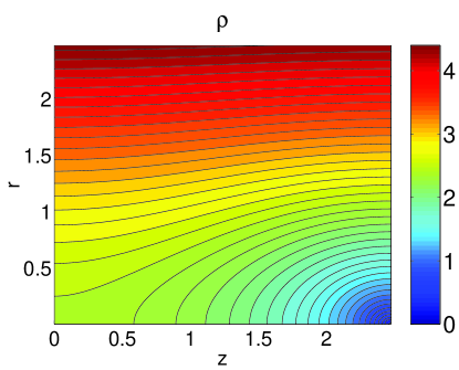
Figure 1: Plot of $\rho$ measured from the $\lambda=3.9$ string solution.

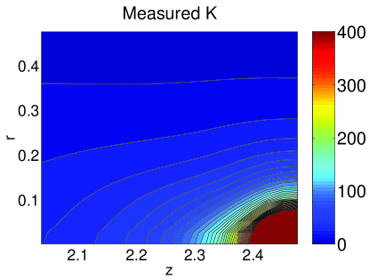
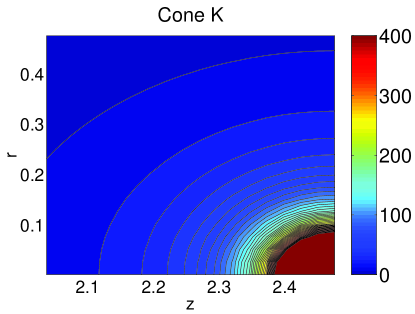
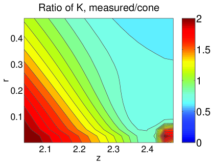
Figure 2: Plot showing $K$, the scalar curvature invariant, measured from the string ($\lambda=3.9$) compared to the cone prediction. The ratio is also shown, and we see good agreement slightly away from the apex, where finite $\lambda$ ‘resolves’ the cone. Moving far from the cone ie. $z<2.1$ or $r>0.4$ the cone is no longer a good approximation, the actual curvature becoming more homogeneous in $z$.

In figure 1 we plot the function $\rho$ against $r,z$ for the most non-uniform solution found numerically, with $\lambda=3.9$. We see very clearly the correct qualitative behaviour of $\rho$ for a cone near to the minimal sphere at $r=0,z=L_{n}$, where $\rho$ has its minimum. The degree to which the cone is ‘resolved’ can be estimated from this minimum value. For the value of $\lambda$ plotted in the figure, $\rho_{min}=0.27$. This indicates that the cone will be a good approximation for $\rho>\rho_{min}$, but $\rho<<L_{n}$, the characteristic scale of the compactification.

Quantities involving only $\rho$ provide the easiest numerical comparisons. In the next section we see that computing $\chi$ from $A,B,C$ involves further processing, and thus tests only involving $\rho$ should be more robust. A non-trivial test of the cone conjecture, simply involving $\rho$ is a comparison of the Kretschmann curvature scalar with the cone prediction. For the cone metric (4) one finds,

$$K=R^{\mu\nu\alpha\beta}R_{\mu\nu\alpha\beta}=\frac{48}{\rho^{4}}$$ (8)

One can compute the same quantity for the numerical solutions directly from $A,B,C$ and the two are plotted in figure 2 for the region near the waist. We also plot the ratio of these quantities in the same figure. We see that at the waist agreement is lost, as we expect because we are at finite $\lambda$. However, moving away from the apex, agreement seems to be good, considering the relatively low numerical resolution available over such a small subregion of the string solution. The ratio is close to one, and we also see a possible sub-leading behaviour in $r$, and less strongly in $z$ as we move away from the ‘apex’. Moving further from the waist we see the curvature contribution from the cone decays sufficiently that a more homogeneous curvature emerges, as expected for a string.

III.2 Full metric comparison

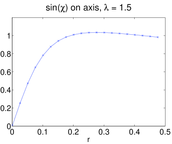
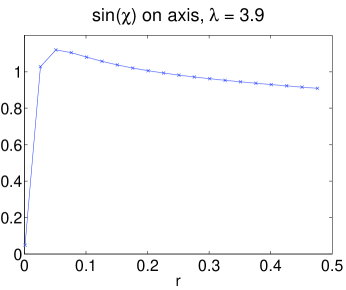
Figure 3: Plots of $\sin{\chi}$ on the $z=L_{n}$ axis measured from string solutions with $\lambda=1.5,3.9$. For the larger $\lambda$ we see the curve become more ‘constant’, and furthermore, the value is remarkably consistent with one, the cone prediction.

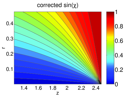
Figure 4: Plot of $\sin{\chi}$ computed from $\lambda=3.9$ string, including normalisation correction to ensure $\sin{\chi}=1$ at $z=L_{n}$, so that $\chi$ can be meaningfully extracted.

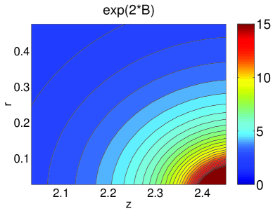
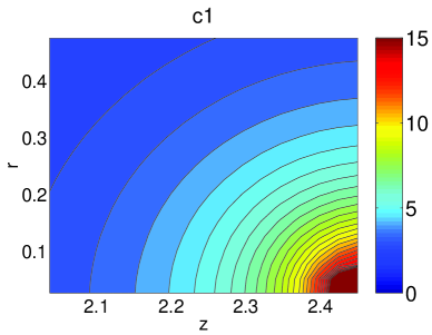
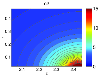
Figure 5: Plots of remaining metric components $c1,c2$ computed from the numerical solution with $\lambda=3.9$ using the ‘corrected’ $\sin{\chi}$. The cone predicts that $c1=c2=e^{2B}$ which is also plotted for comparison. Very good agreement is seen, given that the underlying data is on a lattice of only approximately $20*20$ and resolution effects may give significant numerical errors.

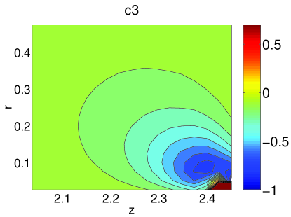
Figure 6: The off-diagonal metric component $c3$ which the cone predicts to be zero. Away from the resolved apex, we see it is indeed much smaller than the values of $c1,c2$ in the previous plot, again being consistent with the cone ansatz.

This curvature invariant indicates the size of the region where we expect good agreement. Now we perform a full metric comparison using $\chi$ as well as $\rho$. However, use of $\chi$ is subtle. For the cone obviously $\sin{\chi}=1$ for $\chi=\pi/2$. However, we are measuring $\sin{\chi}$ directly, not $\chi$, and due to finite $\lambda$ resolving of the cone, and limited numerical resolution, we no longer can expect that $\sin{\chi}=1$ exactly at $z=L_{n}$. In figure 3 we plot $\sin{\chi}$ for two values of $\lambda=1.5,3.9$ at $z=L_{n}$, over the range of $r$ indicated in the previous section to yield good agreement. Not only do we clearly see that for the larger $\lambda$ value $\sin{\chi}$ on the axis $z=L_{n}$ appears to be more constant, but moreover this constant is indeed consistent with one. Bearing in mind the low resolution we regard this as remarkably good agreement. For the lower value of $\lambda$, a constant behaviour is still seen at large $r$, again consistent with one, but there is a larger region near the apex where $\sin{\chi}$ is clearly not a constant, being approximately linear in $r$.

In order to compute (6) we must compute $\chi$ from the $\sin{\chi}$ and obviously this may lead to pathologies, as we see above that the $\sin{\chi}$ measured at $z=L_{n}$ is larger than one at its peak. Therefore, we normalise the $\sin{\chi(r,z)}$ measured by its value on the $z=L_{n}$ axis (which ‘should’ be one, and we have seen does well approximate one) as,

$$\sin{\chi(r,z)}_{corrected} = \sin{\chi(r,z)}/\sin{\chi(r_{0},L_{n})}$$

$$\rho(r_{0},L_{n}) = \rho(r,z)$$ (9)

so we use contours of $\rho$ to find the value on the axis $z=L_{n}$ to normalise by. This tidies up $\chi$ at $z=L_{n}$, and it is difficult to see how to extract $\chi$ without dealing with this issue.

Now we plot $\sin{\chi}_{corrected}$ in figure 4. We see exactly the type of behaviour we would expect, with contours of $\chi$ parameterising an angle near the apex. Then in figure 5 we plot the $dr^{2}$ and $dz^{2}$ components of the metric ($c1,c2$) (6) calculated using the corrected $\chi$. According to the cone conjecture, these components should be equal to each other, and to $e^{2B(r,z)}$, which we also plot in this figure. We see rather remarkable consistency with the cone prediction. The remaining test is that the measured $drdz$ component ($c3$) should be zero, or numerically speaking, much smaller than the $dr^{2},dz^{2}$ components. This is finally plotted in figure 6, and again we see that the prediction is indeed true.

IV Charged strings

Uniform strings electrically charged under a Maxwell field can be constructed from black hole solutions of Einstein-Maxwell-Dilaton theory Gibbons et al. (1995); Gibbons and Maeda (1988); Garfinkle et al. (1991). For small charges non-uniform deformations will exist since the GL instability persists. As the string horizon is an equipotential surface which is “dented” we expect the field to be reduced in the waist region – this is the complementary effect to the appearance of high fields near a “pointed protrusion”. Here we consider whether we can quantify this further, using our concrete example $d=6$.

Unfortunately at this time we know of no generalisation of the cone to include an electric flux. Therefore we simply consider putting a small charge on the cone and neglecting its back-reaction. Making the electric ansatz that the vector potential $A_{t}=\phi(\rho,\chi)$ with other components being zero, one finds,

$$\partial_{\rho}^{2}\phi+\frac{3}{\rho}\partial_{\rho}\phi+\frac{4}{\rho^{2}}\left(\partial_{\chi}^{2}\phi-\cot{\chi}\partial_{\chi}\phi\right)=0$$ (10)

The solution can be separated, $\phi(\rho,\chi)=f(\rho)g(\chi)$ and the resulting equations solved in terms of a separation constant $k$, which we may chose to be positive. The radial equation is easily solved giving,

$$f(\rho)=\rho^{\pm k-1}$$ (11)

and since we wish the back-reaction to be small, we may only take solutions that are regular as $\rho\rightarrow 0$.

Now we consider the angular equation. The horizon, at $\chi=0,\pi$, must be an equipotential surface. Due to the separable form, we see this may either be achieved by $f$ being constant (ie. k = 1), or by $g=0$ at $\chi=0,\pi$. The first case yields only the trivial solution $\phi=const$. The second is more subtle, and we find the solution,

$$g(\chi)=\sin^{2}{\chi}\,F\left(\frac{3-k}{4},\frac{3+k}{4};2;\sin^{2}{\chi}\right)$$ (12)

where $F(a,b;c;x)$ is the hyper-geometric function. Additionally we add the geometric boundary condition at $\chi=\pi/2$, where the differential equation is singular, that $g(\chi)$ be reflection symmetric. The hyper-geometric function is a finite degree polynomial in $\sin^{2}{\chi}$ if $k=3+4n$ with integer $n\geq 0$, and hence has the required reflection symmetry. Indeed we may Taylor expand $g$ about $\chi=\pi/2$ giving,

$$g(\chi)=\frac{\sqrt{\pi}}{\Gamma{\left(\frac{5-k}{4}\right)}\Gamma{\left(\frac{5+k}{4}\right)}}-\frac{2\sqrt{\pi}}{\Gamma{\left(\frac{3-k}{4}\right)}\Gamma{\left(\frac{3+k}{4}\right)}}\cos{\chi}+O(\cos{\chi}^{2})$$ (13)

which confirms that only for these values of $k$ is the reflection boundary condition obeyed.

If we consider the exact cone geometry these modes with $k=3+4n$ clearly blow up at large $\rho$, far from the apex. However, for the non-uniform string, it is unclear what the geometry will be for large $\rho$ and therefore we cannot specify precisely the remaining boundary condition for the radial equation. Instead we assume that the leading order term is not absent in the solution, so the dominant contribution to the potential near the apex is from the lowest $k$, $k=3$, giving,

$$\phi=q\left(\rho\sin{\chi}\right)^{2}+O(\rho^{6})$$ (14)

for constant $q$, the higher corrections coming from $n\geq 1$. Therefore we see the electric field vanishes on the cone horizon confirming our expectation of a reduced field near the apex.

To conclude, we still expect the cone to describe the limiting waist geometry for a weakly charged string. Obviously it would be interesting to understand how this picture changes as the charge is increased to extremality where one expects the GL instability to disappear Gregory and Laflamme (1994, 1995); Horowitz and Maeda (2002).

References

- Gregory and Laflamme (1993) R. Gregory and R. Laflamme, Phys. Rev. Lett. 70, 2837 (1993), eprint [http://arXiv.org/abs]hep-th/9301052.
- Gregory and Laflamme (1988) R. Gregory and R. Laflamme, Phys. Rev. D37, 305 (1988).
- Gubser and Mitra (2000) S. Gubser and I. Mitra (2000), eprint [http://arXiv.org/abs]hep-th/0009126.
- Gubser and Mitra (2001) S. Gubser and I. Mitra, JHEP 08, 018 (2001), eprint [http://arXiv.org/abs]hep-th/0011127.
- Reall (2001) H. Reall, Phys. Rev. D64, 044005 (2001), eprint [http://arXiv.org/abs]hep-th/0104071.
- Gregory and Ross (2001) J. Gregory and S. Ross, Phys. Rev. D64, 124006 (2001), eprint [http://arXiv.org/abs]hep-th/0106220.
- Chamblin et al. (2000) A. Chamblin, S. Hawking, and H. Reall, Phys. Rev. D61, 065007 (2000), eprint [http://arXiv.org/abs]hep-th/9909205.
- Gregory (2000) R. Gregory, Class. Quant. Grav. 17, L125 (2000), eprint [http://arXiv.org/abs]hep-th/0004101.
- Hirayama and Kang (2001) T. Hirayama and G. Kang, Phys. Rev. D64, 064010 (2001), eprint [http://arXiv.org/abs]hep-th/0104213.
- Gibbons and Hartnoll (2002) G. Gibbons and S. Hartnoll, Phys. Rev. D66, 064024 (2002), eprint [http://arXiv.org/abs]hep-th/0206202.
- Kol (2002a) B. Kol (2002a), eprint [http://arXiv.org/abs]hep-th/0206220.
- Gubser (2002) S. Gubser, Class. Quant. Grav. 19, 4825 (2002), eprint [http://arXiv.org/abs]hep-th/0110193.
- Horowitz and Maeda (2001) G. Horowitz and K. Maeda, Phys. Rev. Lett. 87, 131301 (2001), eprint [http://arXiv.org/abs]hep-th/0105111.
- Harmark and Obers (2002) T. Harmark and N. Obers, JHEP 05, 032 (2002), eprint [http://arXiv.org/abs]hep-th/0204047.
- Kol (2002b) B. Kol (2002b), eprint [http://arXiv.org/abs]hep-ph/0207037.
- Kol (2002c) B. Kol (2002c), eprint [http://arXiv.org/abs]hep-th/0208056.
- Smet (2002) P. D. Smet, Class. Quant. Grav. 19, 4877 (2002), eprint [http://arXiv.org/abs]hep-th/0206106.
- Myers (1987) R. Myers, Phys. Rev. D35, 455 (1987).
- Korotkin and Nicolai (1994) D. Korotkin and H. Nicolai (1994), eprint gr-qc/9403029.
- Frolov and Frolov (2003) A. Frolov and V. Frolov (2003), eprint [http://arXiv.org/abs]hep-th/0302085.
- Emparan and Reall (2002) R. Emparan and H. Reall, Phys. Rev. D65, 084025 (2002), eprint [http://arXiv.org/abs]hep-th/0110258.
- Wiseman (2002) T. Wiseman, Phys. Rev. D65, 124007 (2002), eprint [http://arXiv.org/abs]hep-th/0111057.
- Wiseman (2003a) T. Wiseman, Class. Quant. Grav. 20, 1137 (2003a), eprint [http://arXiv.org/abs]hep-th/0209051.
- Wiseman (2003b) T. Wiseman, Class. Quant. Grav. 20, 1177 (2003b), eprint [http://arXiv.org/abs]hep-th/0211028.
- Gibbons et al. (1995) G. Gibbons, G. Horowitz, and P. Townsend, Class. Quant. Grav. 12, 297 (1995), eprint [http://arXiv.org/abs]hep-th/9410073.
- Gibbons and Maeda (1988) G. Gibbons and K. Maeda, Nucl. Phys. B298, 741 (1988).
- Garfinkle et al. (1991) D. Garfinkle, G. Horowitz, and A. Strominger, Phys. Rev. D43, 3140 (1991).
- Gregory and Laflamme (1994) R. Gregory and R. Laflamme, Nucl. Phys. B428, 399 (1994), eprint [http://arXiv.org/abs]hep-th/9404071.
- Gregory and Laflamme (1995) R. Gregory and R. Laflamme, Phys. Rev. D51, 305 (1995), eprint [http://arXiv.org/abs]hep-th/9410050.
- Horowitz and Maeda (2002) G. Horowitz and K. Maeda, Phys. Rev. D65, 104028 (2002), eprint [http://arXiv.org/abs]hep-th/0201241.
- Bohm (1998) C. Bohm, Invent. Math. 134, 147 (1998).
- Herzog and Klebanov (2001) C. P. Herzog and I. R. Klebanov, Phys. Rev. D63, 126005 (2001), eprint hep-th/0101020.