Ghosts in a Mirror

Abstract

We look at some dynamic geometries produced by scalar fields with both the “right” and the “wrong” sign of the kinetic energy. We start with anisotropic homogeneous universes with closed, open and flat spatial sections. A non-singular solution to the Einstein field equations representing an open anisotropic universe with the ghost field is found. This universe starts collapsing from $t\to-\infty$ and then expands to $t\to\infty$ without encountering singularities on its way. We further generalize these solutions to those describing inhomogeneous evolution of the ghost fields. Some interesting solutions with the plane symmetry are discussed. These have a property that the same line element solves the Einstein field equations in two mirror regions $\left|t\right|\geq z$ and $\left|t\right|\leq z$, but in one region the solution has the right and in the other, the wrong signs of the kinetic energy. We argue, however, that a physical observer can not reach the mirror region in a finite proper time. Self-similar collapse/expansion of these fields are also briefly discussed.

I Introduction

Recently some authors have discussed scalar fields with negative kinetic energies (NKE) Carroll ; Gibbons ; Nojiri . In Carroll the authors have studied these fields in connection to the dark matter problem in the universe. Also, since observational evidence does not exclude cosmological models with the pressure to density ratio $<-1$, various models with negative densities were studied recently by several groups negative .

In Gibbons , to motivate these studies, it was argued that one may find several physical examples, such as Lifshitz transitions in condensed matter physics or an unusual dispersion relation for rotons in liquid helium, suggesting that the NKE may appear in nature. Also, negative energy densities may appear in quantum particle creation processes in curved backgrounds Candelas or in squeezed states of the electromagnetic fields Slusher . Their appearance, however, signals usually the unhealthy vacuum instability. Therefore, if the time scale of this instability is too short, the matter cannot serve as viable candidate for the dark energy component Carroll . A different reasoning towards NKE, however, may be applied if one approaches the cosmological singularity problem.

One believes that the emergence of spacetime singularities in General Relativity suggests the breakdown of the theory at its natural scales. At these scales one expects the quantum corrections to take a leading role and save the situation. Different approaches to regularize the singularity have been undertaken. Phenomenologically, and in the light of all the standard singularity theorems, what appears to be the simplest way to tackle the singularity problem is to allow for negative energy densities, and probably some degree of anisotropy and/or inhomogeneity. This would produce the repulsive gravity effects and may smoothen the singularity. Phenomenologically, again, one can associate the negative energy densities with the back reaction of the quantum fluctuations, so that the idea in itself is not that ridiculous. Thus, allowing for NKE may prove to be an interesting approach to spacetime singularities in General Relativity. Here, the problem of the vacuum instability should be irrelevant, and even may become a blessing, for if these exotic fields decay rapidly, after having smoothed the singularity, this well could be a reason as to why we live in a ghost-free world. Consequently, it is worthwhile to have a closer look at some geometries produced by such fields, and we suggest here that one should keep her/his eyes wide open, just in case.

We will be especially interested in dynamical spacetimes in this setting, some static solutions in the ghost sector were presented elsewhere Gibbons ; Gibbons-Rasheed . Just to concentrate on the simplest examples we consider the energy-momentum tensor of a massless scalar field in the following form,

$$T_{\mu\nu}=\epsilon(2\varphi_{,\mu}\varphi_{,\nu}-g_{\mu\nu}\varphi_{,\alpha}\varphi^{,\alpha}),$$ (1)

which is derived from the Lagrangian

$${\cal L}={\cal R}-2\epsilon\varphi_{,\alpha}\varphi^{,\alpha},$$ (2)

and where $\varphi$ is a scalar, ${\cal R}$ is the Ricci scalar and $\epsilon$ may take values $1$ and $-1$. Our metric signature convention is $(-,+,+,+)$. When $\epsilon=1$, the energy-momentum tensor is of a standard form, while $\epsilon=-1$ stands for the ghost field.

II HOMOGENEOUS ANISOTROPIC MODELS

Our starting point is the family of Kantowski-Sachs metrics. We choose these space-times because they combine both the non-trivial curvature as well as the effects of anisotropy. We should note, moreover, that we couldn’t find any other non-pathological, dynamical homogeneous and isotropic spacetime with the ghost fields.

With the energy-momentum tensor given by (1) we find the following formal solution to the Einstein field equations,

$$ds^{2}=-(\frac{2\eta}{t}-k)^{-\alpha}dt^{2}+(\frac{2\eta}{t}-k)^{\alpha}dr^{2}$$

$$+t^{2}(\frac{2\eta}{t}-k)^{1-\alpha}(d\theta^{2}+f_{k}(\theta)^{2}d\phi),$$ (3)

with the scalar field given by

$$\varphi(t)=\frac{1}{2}\sqrt{\frac{1-\alpha^{2}}{\epsilon}}\log\left(\frac{2\eta}{t}-k\right).$$ (4)

Here $k$ is spatial curvature $(k=-1,0,1)$, and

$$f_{k}(\theta)=\left\{\begin{array}[]{ll}\sin\theta&k=1,\\ \theta&k=0,\\ \sinh\theta&k=-1.\end{array}\right.$$ (5)

Now, for $\epsilon=1$ and $|\alpha|<1$, we recover the usual Einstein-dilaton solution given, for example, in AF-VM .

When $\epsilon=-1$ one must continue the scalar field analytically in order to finish with a real field and a non-pathological metric. In this case one may obtain real solutions simply by considering the case $|\alpha|>1$. When $\alpha=0$, however, we must continue analytically the $log$ function. It follows, thus, that it is only possible to obtain real solutions in the homogeneous case when $k\neq 0$. On the other hand, when certain amount of inhomogeneity is introduced the extension of $k=0$ solutions is also possible. We will discuss these cases in the next section.

The two ghost solutions with $\alpha=0$ are:

• $k=1$

  $$ds^{2} = -dt^{2}+dr^{2}-(\eta^{2}+t^{2})(d\theta^{2}+\sin^{2}\theta d\phi^{2}),$$

  $$\varphi(t)=\arctan\left(\frac{\eta}{t}\right),$$

• $k=-1$

  $$ds^{2} = -dt^{2}+dr^{2}+(\eta^{2}+t^{2})(d\theta^{2}+\sinh^{2}\theta d\phi^{2}),$$

  $$\varphi(t)=\arctan\left(\frac{\eta}{t}\right).$$

The solution (• ‣ II) is just the Gibbons-Rasheed’s massless “ghost” wormhole Gibbons-Rasheed with $t$ now being the spacelike and $r$ the timelike co-ordinates. The solution (• ‣ II), however, represents a non-singular anisotropic universe with open spatial sections. Its volume expansion $\Theta$ is :

$$\Theta=\frac{2t}{\eta^{2}+t^{2}}.$$ (8)

Figure 1: Volume expansion of nonsingular universe

The volume deformation reads:

$$\sigma=-\frac{t}{\sqrt{3}(\eta^{2}+t^{2})}$$ (9)

The average scale factor $a(t)=(\eta^{2}+t^{2})^{1/6}$, behaves as $a\propto t^{1/3}$ for $\left|t\right|>>\eta$, proper of a stiff fluid.

The non-singular universe is flat and static as $t\to-\infty$, with the vanishing scalar field. It collapses towards a flat universe at $t=0$, where the scalar stabilizes to a constant, and then expands again to a flat universe as $t\to\infty$, with the vanishing scalar field. The solution (• ‣ II) is definitely too crude to represent even a toy cosmology. But imagine, that the massless scalar field with the NKE is supplemented by an ordinary matter, or by a potential as in Carroll . Then, it may be possible that the evolution of the model at different stages is dominated by either the ghost field or by ordinary matter. Near the singularity, the kinetic terms always dominate the potential, and therefore the short period of the ghost domination may give rise to a regular solution. There could also be situations where both ingredients will just conspire to produce a cosmological constant, as in Gibbons , during some epoch. Such a model could then be an interesting test bench to address the singularity, inflation and the coincidence problem at one go. The realistic model building, however, is far beyond the scope of the present paper.

In a different setting, one can make a connection between the solution (• ‣ II) and the singularity problem in low energy string cosmology. The related models are those of the pre-Big Bang scenario (for a review see, Lidsey ; Gasperini ). One of the main difficulties in these models is the smooth exit from the pre-Big Bang into the post-Big Bang regime. The possibilities of the smooth transitions in the context of the lowest-order effective string action were discussed in Risi . There it was concluded that the transitional singularities at $t=0$ can be avoided for anisotropic backgrounds provided one accepts the sources with negative energy densities. The solution (• ‣ II) therefore represents an exact evolution of such a model near $t=0$.

III Inhomogeneous solutions

When $k=0$, the spatially flat case, the two dimensional line element $(d\theta^{2}+\theta^{2}d\phi^{2})$ can be cast into an explicitly flat form: $dx^{2}+dy^{2}$. In this case the analytical continuation of the scalar field simply does not exist. We, therefore, will allow for a certain degree of inhomogeneity and consider the following form of the plane symmetric solutions,

$$ds^{2}=\frac{1}{\sqrt{t}}e^{f(t,z)}(-dt^{2}+dz^{2})+t(dx^{2}+dy^{2}).$$ (10)

It should be noted that the discussion here can be generalized in a straightforward manner to any $G_{2}$ spacetime with two commuting spacelike Killing vectors by introducing transversal gravitational degrees of freedom in the following form $(e^{P(t,z)}dx^{2}+e^{-P(t,z)}dy^{2})$. The off-diagonal terms may also be included. For the sake of clarity, however, we stick to a simple plane symmetric case, which we feel is sufficient to make our point.

Assuming the geometry (10) the Klein-Gordon equation reads

$${\varphi_{,tt}}+\frac{1}{t}{\varphi_{,t}}-{\varphi_{,zz}}=0,$$ (11)

and when $\varphi(t,z)$ is the solution of this equation, the metric function $f(t,z)$ can be obtained by quadratures:

$$f_{,t} = 2\epsilon t({\varphi_{,t}}^{2}+{\varphi_{,z}}^{2})$$ (12)

$$f_{,z} = -4\epsilon{\varphi_{,t}}{\varphi_{,z}}.$$ (13)

Again, if $\epsilon$ is $1$ we are dealing with the standard scalar field, and when $\epsilon=-1$ it is a ghost. Thus, the NKE solutions are related to the positive kinetic energy solutions by $f\to-f$ transformation.

We consider now two possible solutions to (11):

$$\varphi_{1}=b\;\hbox{arccosh}\left(\frac{z}{t}\right),\qquad{|z|\geq t}$$ (14)

and

$$\varphi_{2}=b\;\hbox{arccos}\left(\frac{z}{t}\right),\qquad{|z|\leq t}.$$ (15)

Note that $\varphi_{1}$ relates to $\varphi_{2}$ by $b\to ib$ transformation even though they “operate” in two different, mirror, regions of spacetime. The positive energy solutions of Einstein equations for $\varphi_{1}$ and $\varphi_{2}$ are:

$$ds^{2}[1]=\frac{1}{{\sqrt{t}}}(\frac{z^{2}}{t}-t)^{-2b^{2}}(-dt^{2}+dz^{2})+t(dx^{2}+dy^{2}),$$ (16)

for $|z|\geq t$, and

$$ds^{2}[2]=\frac{1}{{\sqrt{t}}}(t-\frac{z^{2}}{t})^{2b^{2}}(-dt^{2}+dz^{2})+t(dx^{2}+dy^{2}),$$ (17)

for $|z|\leq t$. It is amazing, however, that the positive and the negative energy solutions interchange when the kinetic energy sign flips over and the power $2b^{2}$ is even: the negative energy solution for $\varphi_{1}$, is given by the line element (17), while the negative energy solution for $\varphi_{2}$ is given by (16). Therefore, the same geometry (16) is induced by either the normal scalar field in region $|z|\geq t$, or by a ghost field in its mirror region $|z|\leq t$. The same applies to (17).

Now, for the solution (16) Ricci scalar is

$${\cal R}=-2b^{2}t^{-3/2}(\frac{z^{2}}{t}-t)^{2b^{2}},$$ (18)

and, for the solution (17),

$${\cal R}=2b^{2}t^{-3/2}(t-\frac{z^{2}}{t})^{-2b^{2}}.$$ (19)

Therefore, the solutions (17) are singular at $t=z$, but (16) are not. Of course, there happen to be singularities at $t=0$ in these expressions, but these are not of our interest in this section. We have further checked the other curvature scalars for (16), such as square and the cube of the Ricci and the Riemann tensors and found those regular at $t=z$. The possibility then arises, to continue the solution (16) as it stands into the region $|z|<t$, by flipping the sign of the action. The spacetime could have looked as depicted in fig. 2 below.

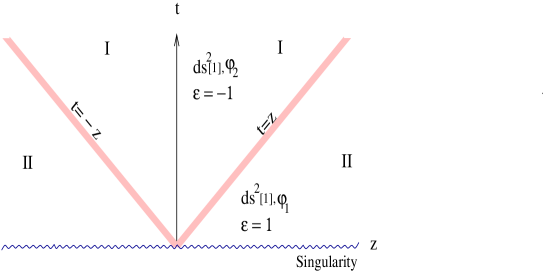
Figure 2: Mirror solutions

The picture looks quite unexpected. One has equivalent geometry on both sides of the mirror line $z=t$, produced by the standard scalar field in the region II, while the same geometry in the region I is produced by a ghost. Technically this happens because the pure imaginary transformation of the scalar field $\varphi_{1}$ into $\varphi_{2}$ produces a real scalar field in a mirror region. It is tempting to call such scalar fields as mirror-ghosts. A different pair of scalar fields which solve the equation (11) and have the mirror ghost properties are $\varphi=b/\sqrt{t^{2}-z^{2}}$ and $\varphi=b/\sqrt{z^{2}-t^{2}}$.

On a closer inspection of the geometry, described by the fig. 2, one finds that the co-ordinates $t$ and $z$ are not that appropriate to describe the situation. It is convenient to introduce the following chart $t=u^{n}+v^{n}$ and $z=u^{n}-v^{n}$, where $n=1/(1-2b^{2})$ Feinstein , and since we have insisted that $2b^{2}$ is even, the power $n$ must be negative. It is then easy to see that the surface $z=t$ corresponds to $v^{n}=0$ and it cannot be reached by a physical observer in a finite proper time. Thus the two regions are worlds apart for their internal observers. The “mirror” and the “real” world do not mix up!

We now consider inhomogeneous evolution with nontrivial spatial curvature. To do so, we generalize the $\alpha=0$ solutions of the previous section using the following anzatz:

$$ds^{2}=-dudv+R^{2}(u,v)(d\theta^{2}+f_{k}(\theta)^{2}d\phi^{2}).$$ (20)

with $f_{k}(\theta)$ as defined in Eqn. (5).

With the energy-momentum tensor given by (1) we find the following solution:

$$\varphi(u,v) = \frac{1}{2{\sqrt{\epsilon}}}\ln\left[\frac{(1-{\sqrt{\epsilon}}p)kv-u}{(1+{\sqrt{\epsilon}}p)kv-u}\right],$$ (21)

$$R^{2}(u,v) = \frac{1}{4}[(1-\epsilon p^{2})k^{2}v^{2}-2kvu+u^{2}],$$ (22)

where the parameter $p$ represents the strength of the scalar field. For $k=1$ and $\epsilon=1$ the solution reduces to the one found by Roberts Roberts . It was further thoroughly investigated by various authors in connection with the spherically symmetric scalar field collapse (see, for example, ONT ). In the standard scalar field case, the $k=0$ solutions are flat spacetimes written in plane wave co-ordinates. While, the $k=-1$ represents scalar field collapse/expansion with open geometry where one does not expect black hole formations since the trapped surfaces, if formed, are non-compact. Thus, in the $k=-1$ case one either has a naked singularity or a regular collapse/expansion similar to the case of $k=1$ ONT .

We now consider the phantom solutions ($\epsilon=-1$). These are given by

$$\varphi(u,v)=\hbox{arctan}\left(\frac{pkv}{kv-u}\right).$$ (23)

One can see that the scalar field remains regular everywhere. As a consequence, the scalar curvature is also regular everywhere, but in the geometrical centre $u=0$ and $v=0$:

$${\cal R}=-\frac{8k^{2}p^{2}uv}{[p^{2}k^{2}v^{2}+(kv-u)^{2}]^{2}}.$$ (24)

The higher order curvature invariants behave in a similar way. It is further informative to look at the character of the gradient of the area coordinate $R(u,v)$, i.e., $R_{\alpha}(u,v)R^{\alpha}(u,v)$ Senovilla , which is given by

$$R_{\alpha}R^{\alpha}=k-k^{2}\frac{p^{2}uv}{p^{2}k^{2}v^{2}+(kv-u)^{2}}$$ (25)

The character of the gradient of the area coordinate tells one about trappedness of the surfaces. It follows, that for a given $k$, the character of the area gradient never changes the sign (this doesn’t happen in the non-ghost case where the area gradient is parameter $p$- sensitive). Note, that the change $k=1$ to $k=-1$ corresponds to a change $v\to-v$, or, in $t$ and $r$ co-ordinates ($t=u+v$ and $r=u-v$) to an $r\leftrightarrow t$ interchange, exactly as in the homogeneous cases (• ‣ II), (• ‣ II). Therefore, the solutions with $k=1$ should be seen as dynamical generalizations of the Gibbons-Rasheed worm hole Gibbons-Rasheed , and in fact if looked at carefully in ($t,r$) coordinates represent a time sequence of static worm holes. The solutions with $k=-1$ are inhomogeneous generalizations of the solution (• ‣ II). This interpretation is further stressed by the behaviour of the area gradient, being globally timelike (or null) in the cosmological case, and globally spacelike (or null) in the case of $k=1$.

One can as well look at the scalar curvature singularity at $u=0$ $\cap$ $v=0$ in $t$ and $r$ coordinates. The singularity occurs at $R(t,r)=0$. In the $k=1$ case this surface is given by the equation $r^{2}+p^{2}(t-r)^{2}/4=0$, while in the $k=-1$ case, it is $t^{2}+p^{2}(t-r)^{2}/4=0$. Therefore, the singularity occurs at $t=r=0$.

One may interpret the $k=1$ solution along the lines of ONT . These, then represent non-singular ghost field collapse. The ghost fields should be thought of as imploding from the past null infinity, ($u\to-\infty$). One can easily check that the scalar field vanishes on $v=0$ and is constant along $u=0$ null hypersurfaces. The mass function vanishes on both and so does the flux across these null hypersurfaces. Therefore, one can match $v<0$ and $u>0$ regions with flat spacetime ONT , avoiding singularities. We note that the parameter $p$ plays no essential role here.

IV Conclusions

We have looked at various geometries produced by massless scalar fields both with the positive and the negative kinetic energies. In the homogeneous case, we have shown the existence of non-singular anisotropic solution with open spatial sections and NKE. Assuming inhomogeneous plane symmetry we have found mirror images with exactly the same geometry in different regions of spacetime produced by the scalar fields with positive (in one region) and the negative (in the other) kinetic energies. We have shown, however, that the physical observers from the positive energy region cannot reach the phantom geometry in a finite proper time. We have further generalized the self-similar scalar field dynamical solutions to include both the nontrivial curvature and the negative NKE. These generalize the static ghost worm hole solution to the dynamical case ($k=1$), and the homogeneous anisotropic universe to the inhomogeneous one ($k=-1$). The generalizations introduce singularities which can, probably, be removed by cutting and pasting methods. In particular, if one interprets these solutions as a phantom scalar field collapse, the singularities can be easily removed.

There seems to be much prejudice and suspicion against fields with NKE, especially, due to their possible vacuum instability. The stability is important, however, depending on which problem is to be addressed. If we approach the cosmological singularity, the decay of the fields with NKE should not pose conceptual difficulties. One needs these fields just for short times to smoothen the singularity, and when this is achieved they may as well decay: the ghost appears and then disappears, leaving the world ghost-free. It would be interesting to see whether the phenomenological approach considered here can be obtained from field/string theories, we leave this, however, for future works.

V Acknowledgements

We are grateful to José Senovilla for helpful discussions and valuable comments. A.F. was supported by the University of the Basque Country Grants 9/UPV00172.310-14456/2002, and The Spanish Science Ministry Grant 1/CI-CYT 00172. 310-0018-12205/2000. S.J. acknowledges support from the Basque Government research fellowship.

References

- (1) S. M. Carroll, M. Hoffman and M. Trodden, Can the dark energy equation-of-state parameter w be less than -1?, arXiv:astro-ph/0301273.
- (2) G. W. Gibbons, Phantom Matter and the Cosmological Constant, arXiv: hep-th/0302199.
- (3) S. Nojiri and S.D. Odintsov, Quantum deSitter cosmology and phantom matter, arXiv:hep-th/0303117 .
- (4) R. R. Caldwell, Phys. Lett. B 545, 23 (2002); T. Chiba, T. Okabe and M. Yamaguchi, Phys. Rev. D 62 023511 (2000); B. Boisseau, G. Esposito-Farese, D. Polarski and A. A. Starobinsky, Phys. Rev. Lett. 85, 2236 (2000); V. Faraoni, Int. J. Mod. Phys. D 11, 471 (2002); L. Parker and A. Raval, Phys. Rev. D 60, 123502 (1999) [Erratum-ibid. D 67, 029902 (2003)]; I. Maor, R. Brustein, J. McMahon and P. J. Steinhardt, Phys. Rev. D 65, 123003 (2002); J. G. Hao and X. Z. Li, An attractor solution of phantom field, arXiv:gr-qc/0302100; Varun Sahni and Yuri Shtanov, Braneworld models of dark energy, arXiv:astro-ph/0202346 .
- (5) P. Candelas, Phys. Rev. D 21, 2185 (1980); D. W. Sciama, P. Candelas and D. Deutsch, Adv. Phys. 30, 327 (1981).
- (6) R. E. Slusher, L. W. Hollberg, B. Yurke, J. C. Mertz, J. F. Valley, Phys. Rev. Lett. 55, 2409 (1985).
- (7) G. W. Gibbons and D. A. Rasheed, Nucl. Phys. B 476, 515 (1996).
- (8) A. Feinstein and M. A. Vazquez-Mozo, Phys. Lett. B 441, 40 (1998); A. Buonanno, T. Damour and G. Veneziano, Nucl. Phys. B 543, 275 (1999).
- (9) J. E. Lidsey, D. Wands and E. J. Copeland, Phys. Rept. 337, 343 (2000).
- (10) M. Gasperini and G. Veneziano, Phys. Rept. 373, 1 (2003).
- (11) G. De Risi and M. Gasperini, Phys. Lett. B 521, 335 (2001).
- (12) A. Feinstein and J. Ibañez, Phys. Rev. D 39, 470 (1989).
- (13) Yu. Kozarev, L. Okun and I. Pomeranchuk, Yad. Fiz. 3, 1154 (1966).
- (14) S. L. Glashow, Phys. Lett. B 167, 35 (1986).
- (15) M. D. Roberts, Gen. Rel. Grav. 21, 907 (1989).
- (16) Y. Oshiro, K. Nakamura and A. Tomimatsu, Prog. Theor. Phys. 91, 1265 (1994).
- (17) J. M. Senovilla, Class. Quant. Grav. 19, L113 (2002).