SD-brane gravity fields and rolling tachyons

Abstract:

S(pacelike)D-branes are objects arising naturally in string theory when Dirichlet boundary conditions are imposed on the time direction. SD-brane physics is inherently time-dependent. Previous investigations of gravity fields of SD-branes have yielded undesirable naked spacelike singularities. We set up the problem of coupling the most relevant open-string tachyonic mode to massless closed-string modes in the bulk, with backreaction and Ramond-Ramond fields included. We find solutions numerically in a self-consistent approximation; our solutions are naturally asymptotically flat and time-reversal asymmetric. We find completely nonsingular evolution; in particular, the dilaton and curvature are well-behaved for all time. The essential mechanism for spacetime singularity resolution is the inclusion of full backreaction between the bulk fields and the rolling tachyon. Our analysis is not the final word on the story, because we have to make some significant approximations, most notably homogeneity of the tachyon on the unstable branes. Nonetheless, we provide significant progress in plugging a gaping hole in prior understanding of the gravity fields of SD-branes.

1 Introduction

SD-branes in string theory were first studied by Gutperle and Strominger in ref. [1]. They were introduced as objects arising when Dirichlet boundary conditions on open strings are put on the time coordinate, as well as on spatial coordinates. SD-branes are not supersymmetric objects, which makes them hard to handle but potentially very interesting. The boundary conditions for SD-branes imply that they live for only an “instant” of time, and so the worldvolume is purely spatial. SD-branes should not be confused with instantons, because they live out their lives in Lorentzian signature context. Recent discussion of the relation between SD-branes and instantons may be found in section 6 of ref. [10].

SD-branes are especially interesting objects to study in the context of tachyon condensation, which will be the arena of our investigation. SD-branes are indeed inherently related to the general study of time dependence in string theory. One of the original goals of ref. [1] was in fact to seek examples of gauge/gravity dualities where a time direction on the gravity side is holographically reconstructed by a Euclidean field theory.

There have been several investigations of SD-branes since they were introduced [4, 5, 6, 7, 8, 9, 10]. Most of them involve taking the limit $g_{s}\rightarrow 0$, the regime in which perturbative string computations can be done. As the tachyon rolls down its potential hill, there is a divergence in production of higher mass open string modes [6, 11, 10]. This divergence occurs before the tachyon gets to the bottom of the potential well, as it must because there are no perturbative open string excitations around the true minimum of the tachyon potential [12]. Also, the time taken to convert the energy of the rolling tachyon into these massive open string modes is of order ${\cal{O}}(g_{s}^{0})$ . This analysis was done for a single SD-brane using CFT methods; analysis for production of massive closed string modes was also done [13, 14].

One aspect of SD-brane physics has become clear: that the decoupling limit applied to SD-branes is not a smooth limit like it is for regular D-branes. In particular, as $g_{s}\rightarrow 0$ the brane tachyon becomes decoupled from bulk modes, which were however the most natural modes into which the initial energy of the unstable brane should decay. Then, the endpoint of the rolling tachyon must include a somewhat mysterious substance called “tachyon matter” [15]. Consideration of the full problem with $g_{s}$ finite would presumably eliminate the need for mysterious tachyon matter; this was in fact part of our motivation for this work. Regarding production of closed string massive modes, at very small $g_{s}$, it seemed that there was some debate [13, 14] about the form of a divergence. The results from ref. [14] make clear that the divergence depends on the number of dimensions transverse to the decaying unstable brane: for unstable D$p$-branes with $p<2$ there was a need to invoke a cutoff to get a finite result. In any case, unstable brane decay should presumably be a physically smooth process for $\{g_{s},\ell_{s}\}$ finite.

The point of view that we will be taking is to consider a system of $N$ SD-branes, with $g_{s}N$ large, study the overall centre-of-mass tachyon, and couple it to bulk massless closed string modes. Obviously, it would be nice to understand the full problem including coupling to all massive open and closed string modes, but this is a hard problem beyond our reach. We will make a beginning here with a quantitative analysis involving only the lowest modes in each of the open and closed string sectors. We believe that our approach, while “lowbrow” by comparison to SFT computations, already shows some very interesting physics.

The punchline of our paper will be this: we find nonsingular solutions for the evolution of the open string tachyon coupled to bulk supergravity modes. This plugs a gaping hole in our previous understanding [1, 4, 5] of the supergravity fields arising from a large number of SD-branes. All previous attempts at describing SD-branes in the context of supergravity had found that the corresponding solutions were plagued with naked spacelike singularities. We find that resolution of these singularities is achieved in a conceptually simple way: by including full backreaction on the rolling tachyon.

Our investigation can also be considered to shed light on the question of tachyon cosmology [16] including Ramond-Ramond fields, the effect of which was ignored in previous investigations. Tachyon cosmology itself may not yet provide realistic models for inflation, nonetheless, see recent work including, e.g., refs. [17, 18]. One of the reasons is that, in the low-energy actions used to describe tachyon cosmology dynamics, there is only one length scale — the string length. It would certainly be interesting if a mechanism generating a lower scale for inflation were found within this context. Also, the behavior of inhomogeneities during the later stage of the roll of the tachyon may be a general problem [17]. Tachyon cosmology involving brane-antibrane annihilation may be relevant only to a pre-inflationary period, but it is interesting to analyze the dynamics from the “top-down” perspective in string theory.

The plan of our paper is as follows. We begin by reviewing in section 2 the previous work on gravity fields of SD-branes, and commenting on the nature of singularities found in the past. In section 2.1 we discuss pathologies of the solutions found in refs. [4, 5], where only supergravity fields were considered. In section 2.2 we move to discussing ref. [7], in which an unstable brane probe was coupled to a $d=4$ SD0-brane supergravity background; we generalized their arguments but still find generic singularities in the probe approximation (exceptions are considered in Appendix A). In section 3 we set up the full backreacted problem of interest. The equations are naturally highly nonlinear, and since backreaction is essential we have no desire to ignore it or treat it perturbatively. We need to use a particular homogeneous ansatz to facilitate solution of the equations of motion, and we discuss implications of the ansatz. In section 4 we demonstrate numerical solutions of our backreaction-inclusive equations, and interpret qualitative features found. In particular, we follow carefully the evolution of both the dilaton and curvature invariants. Lastly, in the Discussion section we summarize our conclusions, open issues, and directions of future work.

2 Singular supergravity SD-branes: Review

In the paper [1], a small number of supergravity solutions, thought to be appropriate for a large number $N$ of SD-branes, were presented. Subsequently, the class of supergravity solutions was widened considerably, simultaneously by two groups (refs. [4] and [5]). A later paper showed that these two sets of solutions were equivalent [8], by matching boundary conditions on asymptotic fields and finding the coordinate transformation explicitly.

2.1 Sourceless SD-brane supergravity solutions

The convention of ref. [1], which we will use, is that SD$p$-branes have $(p{+}1)$ worldvolume coordinates. We call these ${\vec{y}}$. There is also the time coordinate $t$, and the $(8{-}p)$ overall transverse coordinates ${\vec{x}}$.

The most general SD$p$-brane supergravity solutions of refs. [4] and [5] can then be written in string frame as follows,

$$ds^{2}_{{\scriptscriptstyle Sp}} = F(t)^{1/2}\beta(t)^{G}\alpha(t)^{H}\left(-dt^{2}+t^{2}dH^{2}_{8-p}({\vec{x}})\right)$$

$$+F(t)^{-1/2}\left[\sum_{i=2}^{p+1}\left({\beta(t)\over\alpha(t)}\right)^{-k_{i}}(dy^{i})^{2}+\left({\beta(t)\over\alpha(t)}\right)^{k_{1}+{\tilde{k}}}(dy^{1})^{2}\right]\,,$$

$$e^{2\Phi} = F(t)^{3-p\over 2}\left({\beta(t)\over\alpha(t)}\right)^{-\sum_{i=2}^{p+1}k_{i}}\ ,$$ (2.1)

$$C^{(p+1)} = \sin\theta\cos\theta\,{C(t)\over F(t)}\,dy^{1}\wedge\cdots\wedge dy^{p+1}\ ,$$

where

$$C(t)\equiv\left({\beta(t)\over\alpha(t)}\right)^{k_{1}}-\left({\beta(t)\over\alpha(t)}\right)^{{\tilde{k}}}\,,\qquad F(t)\equiv\cos^{2}\theta\left({\beta(t)\over\alpha(t)}\right)^{{\tilde{k}}}+\sin^{2}\theta\left({\beta(t)\over\alpha(t)}\right)^{k_{1}}\ ,$$ (2.2)

and

$$\alpha(t)\equiv 1+\left({\frac{\omega}{t}}\right)^{7-p}\,,\quad\beta(t)\equiv 1-\left({\frac{\omega}{t}}\right)^{7-p}\,.$$ (2.3)

The supergravity equations of motion will be satisfied when the exponents satisfy the constraints,

$${\tilde{k}}^{2}+\sum_{i=1}^{p+1}k_{i}^{2}+{7-p\over 4}(H-G)^{2}-4{8-p\over 7-p} = 0\ ,$$

$${\tilde{k}}+\sum_{i=1}^{p+1}k_{i}-{7-p\over 2}(H-G) = 0\ ,$$ (2.4)

$$H+G-{4\over 7-p} = 0\ .$$

The general metric above is not isotropic in the worldvolume directions ${\vec{y}}$. However, from a microscopic point of view, one expects that the supergravity solution would have an isotropic worldvolume. Isotropy in the worldvolume will be restored in the above solution for the choice $-k_{2}=\cdots=-k_{p+1}=k_{1}+{\tilde{k}}\equiv n$. Unfortunately, the isotropy requirement excludes SD-brane solutions with regular Cauchy horizon. In fact, the curvature invariants associated to all isotropic solutions diverge at $t=\pm\omega$ and $t=0$. Consequently, although they possess the right symmetries and “charge”, these solutions do not appear to be well-defined.

Besides, SD-branes should be represented by solutions with, roughly, three distinct regions: the infinite past with incoming radiation only in the form of massless closed strings, an intermediate region with both open and closed strings, and finally the infinite future with dissipating outgoing radiation in the form of massless closed strings. But the supergravity solutions of refs. [1, 4, 5] cannot represent this process, because there are no rules for deciding how to go through the singular regions (see, however, Appendix A where we show that some anisotropic solutions avoid the pathology).

Nevertheless, the isotropic solutions have a positive feature worth noting: they have the correct asymptotics at large time. In the limit that the functions $\alpha(t)$ and $\beta(t)$ become trivial, part of the metric is simply the Milne universe: flat Minkowski space foliated by hyperbolic sections,

$$\lim_{t\rightarrow\pm\infty}ds^{2}_{{\scriptscriptstyle Sp}}=-dt^{2}+t^{2}dH^{2}_{8-p}({\vec{x}})+\sum_{i=1}^{p+2}(d{y}^{i})^{2}.$$ (2.5)

On the other hand, there are (at least) two reasons to suspect that the above solutions are not the final word in the SD-brane supergravity story. The first is that there are one too many parameters in the solution, by comparison to expectations from microscopics of SD-branes [5]. A possible explanation for this may be as follows. In the rest of our paper, we will be showing that the full coupling/backreaction between the open-string tachyon and the closed-string bulk modes is crucial for resolution of spacetime singularities. It is possible that the freedom in the supergravity solutions may correspond to a freedom in picking boundary conditions for the rolling tachyon — the coupling to which was not included in refs. [1, 4, 5].

The most noticeable negative feature of the above solutions is that the isotropic solutions are nakedly singular. Quite generally, nakedly singular spacetimes arising in low-energy string theory come under immediate suspicion, even though they are solutions to the supergravity field equations. No-hair theorems are usually what we rely on in order to be sure that we have the unique supergravity solution, but no-hair theorems are never valid for solutions with naked spacetime singularities. It is worth noting that it has been shown with an explicit counterexample [19] that even no-hair theorems themselves fail for black holes in $d=5$ with mass and angular momentum — and hence the idea of no-hair theorems in all higher dimensions is under suspicion. (Nonetheless, with particular assumptions about field couplings, no-hair theorems can be proven for static asymptotically flat dilaton black holes [20]. Also, uniqueness of the supersymmetric rotating BMPV [21] black hole in $d=5$ has been proven [22].) Even if a no-hair theorem appropriate to the supergravity theory involving SD-branes could be proven, however, the above solutions we have reviewed would be ruled out as candidates because their singularities are uncontrollably nasty. So we have to look elsewhere.

Let us take a brief sidetrip here to comment on the singularity story for supergravity fields of $N{\gg}1$ regular D-branes with timelike worldvolume. Certainly, the geometry of BPS D3-branes is nonsingular, and there are several other pretty situations known in the literature where branes “melt” into fluxes: the sources are no longer needed. However, the disappearance of D-brane sources for supergravity fields only occurs when the branes are BPS. If any energy density above BPS is added to these systems, singularities reappear: this certainly happens for the D3-brane system. Also, in the low-energy approximation to string theory, it is misleading to think of supergravity fields of D$p$-branes as simple condensates of massless closed string modes. The reason is directly analogous to the fact that the Coulomb field of an electron cannot be a photon condensate because the photon is transverse. Similarly, Coulomb Ramond-Ramond fields of D$p$-branes cannot be represented by supergravity fields alone. This river runs deeper: in the decoupling limit, resolution of dilaton and curvature singularities for $p\not=3$ D$p$-branes is in fact provided by the gauge theory on the D-branes [23, 24].

Let us now get back to our SD-branes. The supergravity situation looks similar to that for non-BPS (ordinary) D-branes: it seems that brane modes will be required for singularity resolution. Therefore, we are motivated to try to solve all problems with prior candidate SD-brane spacetimes by solving the coupled system of brane tachyon plus bulk supergravity fields with full backreaction.

2.2 Unstable brane probes in sourceless SD-brane backgrounds

The first progress towards the goal of singularity resolution in SD-brane systems was made by Buchel, Langfelder and Walcher [7]. We now briefly review what is, for our purposes, the most relevant point of their work.

Essentially, they take the reasonable point of view that the process of creation and subsequent decay of a SD$p$-brane must be driven by a single open string mode: the tachyon field denoted $T(t)$, which lives on the associated unstable D$(p{+}1)$-brane. They use the $p=0$ non-dilatonic version of the worldvolume action [25, 26, 27, 28, 15, 29]

$$S_{brane}=-T_{p+1}\int d^{p+2}y\,e^{-\Phi}V(T)\sqrt{-det\,\left({\cal P}G_{\alpha\beta}+\partial_{\alpha}T\partial_{\beta}T\right)}+\mu_{p+1}\int f(T)dT\wedge C^{(p+1)},$$ (2.6)

to study the dynamics of the tachyon and its couplings with bulk (closed string) modes. The operation ${\cal P}$ is for pullback, and $\alpha,\beta=1\ldots(p{+}1)$. In section 3.1 we will comment both on the validity of this type of effective action, and on the expected form for the tachyon potential $V(T)$ and the Ramond-Ramond coupling $f(T)$. For now, we just use it.

The way we look at the calculation of ref. [7] is as follows. Supergravity SD-brane fields should be regarded as arising directly from a large number of unstable branes. Then, using the intuition gained from studying the enhançon mechanism [30], it is natural to use an unstable brane probe to study more substantively the candidate supergravity solutions of refs. [4, 5]. Then, we look for problems arising in the probe calculation. The idea is that whenever the probe analysis goes wrong, it signals a pathology for the gravitational background. There are at least two ways the probe analysis can signal a problem: infinite energy or pressure density for the tachyon may be induced, ($\rho_{probe},p_{probe}\rightarrow\pm\infty$), or there might not exist any reasonable solutions for $T(t)$ across the horizon.

So let us consider inserting an unstable brane probe in a background with fields corresponding to the sourceless SD-brane supergravity fields, eqs. (2.1), of the previous subsection. The equation of motion for the open string tachyon is, generally,

$$(-g_{tt})^{\frac{1}{2}}(g_{y^{i}y^{i}})^{\frac{p}{2}}(g_{y^{1}y^{1}})^{\frac{1}{2}}e^{-\Phi}\frac{\partial V(T)}{\partial T}\Delta^{\frac{1}{2}}$$

$$+ f(T)\,F^{(p+2)}+\frac{d}{dt}\left(\dot{T}\,V(T)\frac{(g_{y^{1}y^{1}})^{\frac{1}{2}}(g_{y^{i}y^{i}})^{\frac{p}{2}}}{e^{\Phi}\Delta^{\frac{1}{2}}(-g_{tt})^{\frac{1}{2}}}\right)=0,$$ (2.7)

where ${\dot{\ }}\equiv d/dt$, our notation for the Ramond-Ramond field strength is $F^{(p+2)}=dC^{(p+1)}$, we have factored out $T_{p+1}$ by including a factor of $g_{s}$ in $C^{(p+1)}$, and we also defined the following expression,

$$\Delta=1+\frac{(\dot{T})^{2}}{g_{tt}}.$$ (2.8)

The question needing attention here is whether or not the tachyon field, regarded as a probe, is well-behaved when inserted in the candidate supergravity backgounds (2.1). Ref. [7] provided a clear answer for the case of a $d=4$ SD0-brane with dilaton field set to zero. Let us now see how this goes.

The $d=4$ SD0-brane background introduced in ref. [1] has the form,

$$g_{tt}=-g^{y^{1}y^{1}}=-\frac{Q^{2}}{\omega^{2}}\frac{t^{2}}{t^{2}-\omega^{2}},\;\;\;\;g_{y^{i}y^{i}}=0,\;\;\;\;g_{xx}=\frac{Q^{2}}{\omega^{2}}t^{2},$$ (2.9)

and

$$F_{2}=Q\epsilon_{2}\,,\quad\Phi=0.$$ (2.10)

This spacetime metric has a regular horizon (a coordinate singularity) at $t=\omega$, and a genuine timelike curvature singularity at $t=0$. The expressions for the energy density ($T^{t}_{t}$) and the pressure ($T^{y^{1}}_{y^{1}}$) associated with the probe are respectively,

$$\rho_{probe}\sim\frac{V(T)}{\Delta^{1/2}}\,,\quad p_{probe}\sim V(T)\Delta^{1/2}.$$ (2.11)

The only time (apart from $t=0$) when the probe limit becomes ill-defined is around $t=\omega$. In fact, in the near horizon limit, the dynamical quantity $\Delta$ satisfies the simple ordinary differential equation

$$\Delta^{2}-\Delta+(t-\omega)\dot{\Delta}=0.$$ (2.12)

This has the general solution

$$\Delta=\frac{t-\omega}{t-\omega+g},$$ (2.13)

where $g$ is a constant of integration. There are two possible solutions at $t=\omega$: $\Delta=0$ ($g\neq 0$) or $\Delta=1$ ($g=0$). Clearly, the case for which $\Delta=0$ corresponds to the probe limit breaking down since the energy density of the unstable brane diverges. The other possibility, $\Delta=1$, implies that the time-derivative of the tachyon diverges on the horizon. This last case is clearly pathological and cannot correspond to a physically relevant tachyon field solution.

The conclusion is that unstable brane probes are not well-defined in the SD0-brane background. Not only are they useless to resolve the timelike singularity at $t=0$ but, worse, they appear to generically induce a spacelike curvature singularity on the horizon at $t=\omega$. That is, if we take the probe story to be a good indicator of the story for the full backreacted problem.

One of our first motivations for the work leading to our paper was to plumb how restricted the conclusions of ref. [7] were. Did this above story work only for bulk couplings of the kind arising for SD0-branes in $d=4$, where no dilaton field appears? Was it true only for the case of SD0-branes, which are a special case for SD$p$-branes since there can be no anistropy in a one-dimensional worldvolume? Are all timelike clothed singularities turned into naked spacelike singularities by probes? Could we even trust the probe approximation to tell us anything about the solution with full backreaction?

The first generalization we considered was to look at an unstable brane probe in the background of the isotropic SD$p$-brane solutions of ref. [5]. However, what we saw there was that the naked spacelike singularities remained naked spacelike singularities; the small effect of the probe could not undo that pathology. Next, we moved to analyzing anisotropic solutions of the form (2.1), those with regular horizons. Some of these are actually completely nonsingular; we analyzed the details of the probe computation in those backgrounds, and the specifics are recorded in Appendix A. The results there are simple to summarize: the solutions with singularities hidden behind horizons do not give rise to conclusions qualitatively different than what we have reviewed here for $d=4$ SD0-branes. The picture therefore remains unsatisfactory.

The upshot, then, is that the probe story does not resolve singularities found for sourceless supergravity SD-brane solutions. So we now move to the full backreacted problem for SD$p$-branes in $d{=}10$, which is the main content of our paper.

3 Supergravity SD-branes with a tachyon source

In this section we find, in the context of supergravity, the equations of motion associated with the real-time (formation and) decay of a clump of unstable D-branes. We begin this section by writing the form of the action which we will use in our analysis. We will concentrate on only the most relevant modes in both the open and closed string sectors; in other words, we keep in our analysis only the (homogeneous) tachyon and massless bulk supergravity fields. Potentially, the effect of massive modes could be encoded in a modified equation of state for the tachyon fluid on the unstable D-brane. We leave for future work the issue of non-homogeneous tachyonic modes, and of massive string modes in both the open and closed string sectors, for the coupled bulk-brane system with full backreaction. In order to use the supergravity approximation here self-consistently, we will take $g_{s}$ small but $g_{s}N$ large, and time-derivatives will be small compared to $\ell_{s}$. We will see that it is simple to choose boundary conditions in our numerical integration such that these remain true for all time.

3.1 Preliminaries: action and equations of motion

For this section we will be able to suppress R-R Chern-Simons terms in writing the bulk action. This is a consistent truncation, to set the NS-NS two-form to zero throughout the evolution of the system of interest, as long as consistency conditions on the R-R fields are satisfied. E.g. for the SD2-brane system with R-R field $C^{(3)}$ activated, it is necessary to make certain that $dC^{(3)}\wedge dC^{(3)}=0$ in order not to activate the NS-NS two-form and the accompanying Chern-Simons terms. Other cases are related to this one by T-duality. Therefore, we allow only electric-type coupling of the SDp-brane to $C^{(p+1)}$ (or equivalently magnetic-type coupling to $C^{(7-p)}$). Later we will show that this ansatz is physically consistent provided we assume that there is $ISO(p+1)$ symmetry along the worldvolume of the SDp-brane, the object we are interested in. This is equivalent to considering only the lowest-mass tachyon, i.e., not allowing any excitations of the brane tachyon along the spatial worldvolume directions. Of course, the R-R field strengths are then very simple: $G^{(p+2)}=dC^{(p+1)}$, and the string frame bulk action takes the form [31]

$$S_{{\rm{bulk}}}={\frac{1}{16\pi G_{10}}}\int d^{10}x\,\sqrt{-g}\left\{e^{-2\Phi}\left[{\cal R}+4(\partial\Phi)^{2}\right]-{\frac{1}{2}}\left|dC^{p+1}\right|^{2}\right\}\,,$$ (3.14)

where ${\cal R}$ is the Ricci scalar. We use a mostly plus signature. In the above conventions, the R-R field solutions automatically get a factor of $g_{s}$ (as we mentioned also in the previous subsection), and

$$16\pi G_{10}=(2\pi)^{7}g_{s}^{2}\ell_{s}^{8}\,,\quad\tau_{Dp}={\frac{1}{g_{s}(2\pi)^{p}\ell_{s}^{p+1}}}.$$ (3.15)

Our analytical and numerical results in following sections will be given in string frame. If desired, it is easy to convert to Einstein frame – with metric ${\tilde{g}}_{\mu\nu}$ – with canonical normalization of the metric and positive dilaton kinetic energy, by using the standard $d=10$ conformal transformation

$${\tilde{g}}_{\mu\nu}=e^{-(\Phi-\Phi_{\infty})/2}g_{\mu\nu}.$$ (3.16)

Stress-tensors are defined in Einstein frame,

$${\tilde{T}}_{\mu\nu}\equiv{\frac{-1}{\sqrt{-{\tilde{g}}}}}{\frac{\delta S_{{\rm{matter}}}}{\delta{\tilde{g}}^{\mu\nu}}},$$ (3.17)

with the usual

$${\tilde{T}}_{\mu\nu}\left[\Phi\right] = {\frac{1}{2}}\left[\partial_{\mu}\Phi\partial_{\nu}\Phi-{\frac{1}{2}}{\tilde{g}}_{\mu\nu}({\tilde{\partial\Phi}})^{2}\right]\,,$$ (3.18)

$${\tilde{T}}_{\mu\nu}\left[C^{p+1}\right] = {\frac{1}{2(p+1)!}}e^{(3-p)\Phi/2}\left[{\tilde{G}}_{\mu}^{\ \lambda_{2}\ldots\lambda_{p+2}}G_{\nu\lambda_{2}\ldots\lambda_{p+2}}-{\frac{1}{2(p+2)}}{\tilde{g}}_{\mu\nu}{\tilde{G}}^{2}\right].$$ (3.19)

We can transform to string-frame “Einstein” equation using standard formulæ

$${\tilde{{\cal R}}}_{\mu\nu}-{\frac{1}{2}}{\tilde{g}}_{\mu\nu}{\tilde{{\cal R}}}-{\frac{1}{2}}\left[\partial_{\mu}\Phi\partial_{\nu}\Phi-{\frac{1}{2}}{\tilde{g}}_{\mu\nu}({\tilde{\partial\Phi}})^{2}\right]$$ (3.20)

$$= {\cal R}_{\mu\nu}-{\frac{1}{2}}g_{\mu\nu}{\cal R}+2\left[\nabla_{\mu}\partial_{\nu}\Phi-g_{\mu\nu}\nabla^{2}\Phi+g_{\mu\nu}(\partial\Phi)^{2}\right].$$

For all matter fields except the dilaton, it is therefore obvious that string frame “stress-tensors” take the form

$$T_{\mu\nu}={\frac{-1}{\sqrt{-g}}}{\frac{\delta S_{\rm matter}}{\delta g^{\mu\nu}}}.$$ (3.21)

For the dilaton we find

$$T^{\mu}_{\ \nu}\left[\Phi\right]=2\left[-\nabla^{\mu}\partial_{\nu}\Phi+g^{\mu}_{\ \nu}\nabla^{2}\Phi-g^{\mu}_{\ \nu}(\partial\Phi)^{2}\right]\,,$$ (3.22)

and, obviously, familiar energy conditions for bulk fields are only satisfied in Einstein frame, not string frame.

For the bulk field equations, we must include coupling to the brane tachyon — this is of course an important point of our paper. Hence, we now turn to the brane action. The brane theory is that appropriate to unstable D($p+1$)-branes, for SD$p$-branes. We consider $N$ branes. At low energy, the overall $U(1)$ center-of-mass tachyon $T$ couples as follows:

$$S_{{\rm{brane}}}={\frac{\Lambda}{16\pi G_{10}}}\left\{\int dtd^{p+1}y\left[-\ e^{-\Phi}\sqrt{-A}V(T)\right]+\int f(T)dT\wedge C^{p+1}\right\}\,,$$ (3.23)

where the matrix $A_{\alpha\beta}$ is defined as

$$A_{\alpha\beta}={\cal{P}}\left(G_{\alpha\beta}+B_{\alpha\beta}\right)+F_{\alpha\beta}+\partial_{\alpha}T\partial_{\beta}T\,,$$ (3.24)

where ${\cal{P}}$ stands for pullback. For the constants, our conventions are that $T$ is normalized like $F_{\alpha\beta}$, and also

$$\Lambda\equiv{\frac{N\mu_{p+1}}{g_{s}}}(16\pi G_{10})=(Ng_{s})(2\pi\ell_{s})^{6-p}.$$ (3.25)

Notice that $\Lambda$ is proportional to $g_{s}N$. This will be the sole continuous control parameter associated with the physics of our final solutions for the coupled tachyon-supergravity system.

It is important to know when we can expect to trust the action we use. Our approach consists in assuming that the kinetic terms of the open string tachyon field are re-summed to take a Born-Infeld–like form. Strictly speaking, this has only be shown to be a valid claim late in the tachyon evolution. We refer the reader to ref. [29] for more details on the limits in which this approximation holds (see also ref. [32]). The functions $V(T)$ and $f(T)$ are therefore not known exactly at all times. For definiteness in our numerical analysis, we will choose a specific form and assume that the dynamics of the tachyon is governed by eq. (3.23). For a SD-brane, we make the choice $V(T)=1/\cosh(T/\sqrt{2})=|f(T)|$ which has been shown to be the correct large-$T$ behavior of the couplings. Our results turn out to be quite robust, in that their qualitative features do not depend on the precise form of $V(T)$ and $f(T)$.

For the remainder of our discussion it will be convenient to use static gauge, which is an appropriate gauge choice for our problem of interest. Therefore, in the following, we will be rather cavalier about dropping pullback signs.

When we get to solving the coupled brane-bulk equations, it will be convenient to allow for a density of branes, denoted $\rho_{\perp}$, in the transverse space:

$$\int_{{\rm{brane}}}dtd^{p+1}y\longrightarrow\int_{{\rm{bulk}}}dtd^{p+1}xd^{8-p}x\rho_{\perp}\,.$$ (3.26)

Therefore our brane action becomes

$$S_{{\rm{brane}}}={\frac{\Lambda}{16\pi G_{10}}}\int d^{10}x\rho_{\perp}\left\{-V(T)\sqrt{-A}e^{-\Phi}+f(T)\epsilon^{\lambda_{1}\ldots\lambda_{p+2}}C_{[\lambda_{2}\ldots\lambda{p+2}}\partial_{\lambda_{1}]}T\right\},$$ (3.27)

where $\epsilon$ is the worldvolume permutation tensor with values $(0,\pm 1)$.

We are now ready to write down the coupled field equations. The simplest bulk equation to pick off is the dilaton. In string frame we see immediately that

$$\nabla^{2}\Phi-(\partial\Phi)^{2}+{\frac{1}{4}}{\cal R}={\frac{1}{8}}\left({\frac{\Lambda\rho_{\perp}}{\sqrt{-g}}}\right)e^{+\Phi}V(T)\sqrt{-A},$$ (3.28)

and for the Ramond-Ramond field

$$\nabla_{\mu}G^{\mu\lambda_{2}\ldots\lambda_{p+2}}=-\left({\frac{\Lambda\rho_{\perp}}{\sqrt{-g}}}\right)f(T)\epsilon^{\mu\lambda_{2}\ldots\lambda_{p+2}}\partial_{\mu}T.$$ (3.29)

For the metric equation of motion (string frame “Einstein” equations), it is convenient to define

$${\cal R}^{\mu}_{\ \nu}={\hat{T}}^{\mu}_{\ \nu}\equiv T^{\mu}_{\ \nu}-{\frac{1}{8}}T^{\lambda}_{\lambda}.$$ (3.30)

Therefore, we have

$${\hat{T}}^{\mu}_{\ \nu}[\Phi]=-2\nabla^{\mu}\partial_{\nu}\Phi-{\frac{1}{4}}g^{\mu}_{\ \nu}\nabla^{2}\Phi+{\frac{1}{2}}(\partial\Phi)^{2}g^{\mu}_{\ \nu}.$$ (3.31)

For the brane stress-tensor, we need to figure out the dependence of $\sqrt{-A}$ on $g_{\mu\nu}$ (the Wess-Zumino term clearly does not contribute). We find

$$T^{\mu}_{\ \nu}[T]=-{\frac{1}{2}}e^{\Phi}\left({\frac{\Lambda\rho_{\perp}}{\sqrt{-g}}}\right)V(T)\sqrt{-A}(A^{-1})^{\alpha\mu}g_{\alpha\nu}\,,$$ (3.32)

$${\hat{T}}^{\mu}_{\ \nu}[T]=-{\frac{1}{2}}e^{\Phi}\left({\frac{\Lambda\rho_{\perp}}{\sqrt{-g}}}\right)V(T)\sqrt{-A}\left[(A^{-1})^{\alpha\mu}g_{\alpha\nu}-{\frac{1}{8}}g^{\mu}_{\nu}(A^{-1})^{\lambda\sigma}g_{\lambda\sigma}\right]\,.$$ (3.33)

The other object we need for the metric equation of motion is

$${\hat{T}}^{\mu}_{\ \nu}[C]={\frac{1}{2(p+1)!}}e^{2\Phi}G^{\mu\lambda\ldots\sigma}G_{\nu\lambda\ldots\sigma}-{\frac{(p+1)}{16}}e^{2\Phi}{\frac{G^{2}}{(p+2)!}}g^{\mu}_{\ \nu}\,.$$ (3.34)

Lastly, for the tachyon we find the equation of motion

$${\frac{dV}{dT}}e^{-\Phi}\sqrt{-A}-\partial_{\mu}\left[V(T)e^{-\Phi}\sqrt{-A}(A^{-1})^{\mu\alpha}\partial_{\alpha}T\right]+f(T)\epsilon^{\mu\ldots\lambda}G_{\mu\ldots\lambda}=0\,.$$ (3.35)

In the Discussion section we will make some remarks about the robustness of these equations.

3.2 The homogeneous brane self-consistent ansatz

As pointed out earlier, we are interested in time-dependent processes by which massless Type IIa or Type IIb supergravity fields are sourced by an open-string tachyon mode on the worldvolume of an unstable brane. A reasonable assumption is that the gravitational background generated by backreaction of the rolling tachyon is of the form

$$ds^{2}=-dt^{2}+a(t)^{2}d\Sigma^{2}_{p+1}(k_{\parallel})+R(t)^{2}d\Sigma^{2}_{8-p}(k_{\perp})\,,$$ (3.36)

where the $n$-dimensional Euclidean metric $d\Sigma^{2}_{n}(k)$ is

$$d\Sigma^{2}_{n}(k)=\left\{\begin{array}[]{ll}d\Omega^{2}_{n}&{\rm for}\;k=+1\\ dE_{n}^{2}&{\rm for}\;k=0\\ dH^{2}_{n}&{\rm for}\;k=-1\ ,\end{array}\right.$$ (3.37)

where $d\Omega^{2}_{n}$ is the unit metric on $S^{n}$, $dE_{n}^{2}$ the flat Euclidean metric, and $dH^{2}_{n}$ the ‘unit metric’ on $n$–dimensional hyperbolic space $H^{n}$. The corresponding symmetry groups are

$$\left\{\begin{array}[]{ll}SO(n+1)&{\rm for}\;k=+1\\ ISO(n)&{\rm for}\;k=0\\ SO(1,n)&{\rm for}\;k=-1\ .\end{array}\right.$$ (3.38)

For $k{=}\pm 1$ we obviously require that $n\geq 2$.

We note that the ansatz (3.36), for $k_{\perp}=-1$ and $k_{\parallel}=0$, appears, after using an appropriate change of coordinates, to be equivalent to that considered for supergravity SD-branes in ref. [5]. One can show that this is actually not the case. In order to bring solutions of the form (3.36) with $-\infty<t<+\infty$ to the form introduced in ref. [5] we must find a change of coordinates such that

$$dt^{2}=d\tau^{2}\,F(\tau)^{1/2}(\beta(\tau)\alpha(\tau))^{\frac{2}{7-p}}\left(\frac{\beta(\tau)}{\alpha(\tau)}\right)^{(k_{1}+\tilde{k})(p-1)/(7-p)},$$ (3.39)

where $-\infty<\tau<+\infty$. It turns out that for all values of the parameters associated with the isotropic supergravity solutions, such a change of coordinates does not exist. However, the main feature of our analysis is that we are allowing for modifications of SD-brane physics in the region close to the spacelike worldvolume (the region around $t=0$ for the system of coordinates we use). It should therefore have been expected that our new solutions are not included in those presented in ref. [5]. However, we do expect the asymptotics to agree.

To be physically relevant, solutions should be asymptotically flat. For example, SD-brane gravity solutions will be such that

$$\lim_{t\rightarrow\pm\infty}\dot{a}(t)=0\,,\quad\lim_{t\rightarrow\pm\infty}\dot{R}(t)=1\,,$$ (3.40)

for $k_{\parallel}=0$ and $k_{\perp}=-1$. We will also see in our numerical analysis that only some values of $k_{\perp}$ and $k_{\parallel}$ are allowed. Also, we expect that for the dilaton and R-R field

$$\lim_{t\rightarrow\pm\infty}{\dot{C}}(t)=0\,,\quad\lim_{t\rightarrow\pm\infty}{\dot{\Phi}}(t)=0.$$ (3.41)

By inspection of the tachyon equation of motion (3.35), we see that the electric- (or magnetic-) only ansatz referred to at the beginning of this section will be obviously consistent if we only allow worldvolume time-derivatives. This is tantamount to imposing an $ISO(p+1)$ symmetry on the worldvolume. Ref. [33] argues that spatial inhomogeneities of the tachyon field will play an important role in the decay (a view which is also supported, although using a different line of reasoning, by the results of ref. [34, 17]). It will be interesting to investigate the full importance of such effects in the context of our effective supergravity analysis. We will include a discussion of the nontrivial issues raised in the Discussion section.

It turns out that the equations for the combined bulk-brane evolution in the time-dependent system are complicated enough to require numerical solution. For this reason, we will not be able to accommodate the most natural ansatz $\rho_{\perp}=\delta({\vec{x}})$. Instead, we will use the “smeared” ansatz also used by Buchel et al. in ref. [7],

$$\rho_{\perp}=\rho_{0}\sqrt{g_{\perp}}\,.$$ (3.42)

Note that in this ansatz, the implicit time dependence in the transverse metric components is not varied in producing the equation of motion, rather it is only taken into consideration at the end of the calculation. Also, a smeared brane source does not contribute stress-energy perpendicular to the worldvolume, which is in the directions $t\,,{\vec{y}}$. It should be noted that the effect of using this ansatz will be minimized by using a small value for the density parameter $\rho_{0}$. Of course, the aim when using such an ansatz is to get rid of any brane action dependence on the transverse coordinates ${\vec{x}}$.

We should remark that supergravity solutions corresponding to unstable D-brane systems have been found before [35]. Their solutions are time-independent, a feature which might seem rather unreasonable since they are, after all, supposed to describe unstable objects. Typically, these solutions are nakedly singular; there is no horizon. For reasons discussed previously, these solutions would therefore justifiably be regarded with some level of suspicion. Possibly, we should really regard these solutions as fixed-time snap-shots of the unstable brane system during its evolution. They do however reflect one desirable feature: taking into account warping of space in the directions transverse to the unstable branes.

What we really want is a sort of hybrid of that approach – where transverse dependence is the only dependence – and what we are doing here – where time dependence is all there is. This is something we postpone to a future investigation; remarks on this will be given in the Discussion section.

Let us now get back to the simplified ansatz, and just go ahead and solve it. We are therefore interested in the precise system of ordinary differential equations for our coupled tachyon-supergravity system. Using the form $C_{12\ldots p+1}\equiv C(t)$ (which is consistent with our ansatz) the equation of motion for the R-R field (3.29) becomes

$${\ddot{C}}+{\dot{C}}\left[(8-p){\frac{{\dot{R}}}{R}}-(p+1){\frac{{\dot{a}}}{a}}\right]=\lambda a^{p+1}f(T){\dot{T}}.$$ (3.43)

Now let us find the dilaton equation of motion. A useful identity is

$${\cal R}=5(\partial\Phi)^{2}-{\frac{9}{2}}\nabla^{2}\Phi+{\frac{(3-p)}{8(p+2)!}}e^{2\Phi}G^{2}+{\frac{1}{8}}\left({\frac{\Lambda\rho_{\perp}}{\sqrt{-g}}}\right)e^{\Phi}V(T)\sqrt{-A}(A^{-1})^{\lambda\sigma}g_{\lambda\sigma}\,,$$ (3.44)

with which the dilaton equation of motion can be written,

$$2(\partial\Phi)^{2}-\nabla^{2}\Phi={\frac{(p-3)}{4(p+2)!}}e^{2\Phi}G^{2}+\left({\frac{\Lambda\rho_{\perp}}{\sqrt{-g}}}\right)e^{\Phi}V(T)\sqrt{-A}\left[1-{\frac{1}{4}}(A^{-1})^{\lambda\sigma}g_{\lambda\sigma}\right]\,.$$ (3.45)

This last expression is simply the Einstein frame equation of motion. So the dilaton in our ansatz satisfies

$${\ddot{\Phi}}+{\dot{\Phi}}\left[(8-p){\frac{{\dot{R}}}{R}}+(p+1){\frac{{\dot{a}}}{a}}\right]-2{\dot{\Phi}}^{2}$$

$$={\frac{(3-p)}{4}}\left({\frac{e^{\Phi}{\dot{C}}}{a^{(p+1)}}}\right)^{2}+{\frac{\lambda}{4}}e^{\Phi}V(T)\left[(3-p)\sqrt{\Delta}-{\frac{1}{\sqrt{\Delta}}}\right]\,.$$ (3.46)

This will be used whenever double time-derivatives of the dilaton need to be substituted for.

With $T=T(t)$ we find that the dynamics of the tachyon field is governed by

$${\ddot{T}}=\Delta\left\{{\dot{\Phi}}{\dot{T}}-{\dot{T}}\left[(p+1){\frac{\dot{a}}{a}}\right]-{\frac{1}{V(T)}}{\frac{dV(T)}{dT}}+{\frac{f(T)}{V(T)}}{\dot{C}}e^{\Phi}a^{-(p+1)}\sqrt{\Delta}\right\}\,,$$ (3.47)

where $\Delta=1-\dot{T}^{2}$. In this paper we will be assuming that $|f(T)|=V(T)$, a statement which has been shown to be correct only at past and future asymptopia. However, we have also done numerical experiments which show that some breaking of this relation at intermediate times (near the hilltop) does not change the important features of our solutions.

We now turn to the equations of motion for the metric components $a(t)$ and $R(t)$. For the stress-tensors, eliminating second order derivatives in matter fields, we have

$${\hat{T}}^{t}_{\ t} \!= \!4({\dot{\Phi}})^{2}-2{\dot{\Phi}}\left[(p+1){\frac{{\dot{a}}}{a}}+(8-p){\frac{{\dot{R}}}{R}}\right]+{\frac{(5-2p)}{4}}\left({\frac{e^{\Phi}{\dot{C}}}{a^{p+1}}}\right)^{2}$$ (3.49)

$$\qquad\qquad+{\frac{1}{4}}\lambda e^{\Phi}V(T)\left[(7-2p)\sqrt{\Delta}-{\frac{4}{\sqrt{\Delta}}}\right]\,,$$

$${\hat{T}}^{y}_{\ y} \!= \!2{\dot{\Phi}}{\frac{{\dot{a}}}{a}}-{\frac{1}{4}}\left({\frac{e^{\Phi}{\dot{C}}}{a^{p+1}}}\right)^{2}-{\frac{1}{4}}\lambda e^{\Phi}V(T)\sqrt{\Delta}\,,$$ (3.50)

$${\hat{T}}^{x}_{\ x} \!= \!2{\dot{\Phi}}{\frac{{\dot{R}}}{R}}+{\frac{1}{4}}\left({\frac{e^{\Phi}{\dot{C}}}{a^{p+1}}}\right)^{2}+{\frac{1}{4}}\lambda e^{\Phi}V(T)\sqrt{\Delta}\,.$$ (3.51)

The components of the Ricci tensor are easily evaluated:

$${\cal R}^{t}_{\ t} = (p+1){\frac{\ddot{a}}{a}}+(8-p){\frac{\ddot{R}}{R}}\,,$$ (3.52)

$${\cal R}^{y}_{\ y} = {\frac{\ddot{a}}{a}}+(8-p){\frac{\dot{a}}{a}}{\frac{\dot{R}}{R}}+p\left[\left({\frac{\dot{a}}{a}}\right)^{2}+{\frac{k_{\parallel}}{a^{2}}}\right]\,,$$ (3.53)

$${\cal R}^{x}_{\ x} = {\frac{\ddot{R}}{R}}+(p+1){\frac{\dot{a}}{a}}{\frac{\dot{R}}{R}}+(7-p)\left[\left({\frac{\dot{R}}{R}}\right)^{2}+{\frac{k_{\perp}}{R^{2}}}\right]\,.$$ (3.54)

For the (string-frame) “Einstein” equations, the time, longitudinal and transverse components are respectively

$$(p+1){\frac{\ddot{a}}{a}}+(8-p){\frac{\ddot{R}}{R}} = +4({\dot{\Phi}})^{2}-2{\dot{\Phi}}\left[(p+1){\frac{{\dot{a}}}{a}}+(8-p){\frac{{\dot{R}}}{R}}\right]$$ (3.56)

$$+{\frac{(5-2p)}{4}}\left({\frac{e^{\Phi}{\dot{C}}}{a^{p+1}}}\right)^{2}+{\frac{1}{4}}\lambda e^{\Phi}V(T)\left[(7-2p)\sqrt{\Delta}-{\frac{4}{\sqrt{\Delta}}}\right]\,,$$

$${\frac{\ddot{a}}{a}}=-(8-p){\frac{\dot{a}}{a}}{\frac{\dot{R}}{R}}-p\left[\left({\frac{\dot{a}}{a}}\right)^{2}+{\frac{k_{\parallel}}{a^{2}}}\right]+2{\dot{\Phi}}{\frac{{\dot{a}}}{a}}-{\frac{1}{4}}\left({\frac{e^{\Phi}{\dot{C}}}{a^{p+1}}}\right)^{2}-{\frac{1}{4}}\lambda e^{\Phi}V(T)\sqrt{\Delta}\,,$$ (3.57)

$${\frac{\ddot{R}}{R}}=-(p+1){\frac{\dot{R}}{R}}{\frac{\dot{a}}{a}}-(7-p)\left[\left({\frac{\dot{R}}{R}}\right)^{2}+{\frac{k_{\perp}}{R^{2}}}\right]+2{\dot{\Phi}}{\frac{{\dot{R}}}{R}}+{\frac{1}{4}}\left({\frac{e^{\Phi}{\dot{C}}}{a^{p+1}}}\right)^{2}+{\frac{1}{4}}\lambda e^{\Phi}V(T)\sqrt{\Delta}\,.$$ (3.58)

In the end we have a system of five second order coupled ordinary differential equations for $\{T,C,\Phi,a,R\}$ as functions of $t$. These are respectively equations (3.47), (3.43), (3.2), (3.57) and (3.58). For consistency this system of equations must be supplemented with the first-order constraint

$$\begin{array}[]{l}{\displaystyle{\frac{1}{\lambda e^{\Phi}}\left\{2(p+1)(8-p)\frac{\dot{a}}{a}\frac{\dot{R}}{R}+p(p+1)\left[\left(\frac{\dot{a}}{a}\right)^{2}+\frac{k_{\parallel}}{a^{2}}\right]+(7-p)(8-p)\left[\left(\frac{\dot{R}}{R}\right)^{2}+\frac{k_{\perp}}{R^{2}}\right]\right.}}\\ \qquad\qquad{\displaystyle{\left.-4\dot{\phi}\left[(p+1)\frac{\dot{a}}{a}+(8-p)\frac{\dot{R}}{R}-\dot{\phi}\right]-\frac{1}{2}\left(\frac{e^{\Phi}\dot{C}}{a^{p+1}}\right)^{2}\right\}}}={\displaystyle{\frac{V(T)}{\sqrt{\Delta}}}}\end{array}$$

obtained by plugging eqs. (3.57) and (3.58) in eq. (3.56). Of course, if this last equation is satisfied at $t=0$ it will be for all times.

4 The roll of the tachyon

We refer to a supergravity SD-brane as the field configuration generated by a system composed of a large number, $N$, of microscopic SD-branes. As emphasized in section 3.2, there is a single continuous parameter that controls the dynamics of these fields, i.e., $\lambda=\rho_{0}\Lambda$. This is the parameter that determines the relative importance of the unstable brane source. Clearly, for $\lambda\rightarrow 0$ the open string tachyon decouples from the bulk fields (no backreaction) and the corresponding supergravity solutions will presumably be the singular ones found in refs. [1, 4, 5].

In this section we present solutions with the symmetries of SD-branes and a non-vanishing $\lambda$. We demonstrate that they are generically non-singular.

4.1 Tachyon evolution in flat space

The solutions relevant for SD-brane physics in Type II a,b superstring theory could be the ones corresponding to an open string tachyon evolving from

$$\lim_{t\rightarrow-\infty}T(t)=+\infty$$ (4.59)

to

$$\lim_{t\rightarrow+\infty}T(t)=-\infty$$ (4.60)

in a symmetric runaway potential of the form shown on figure 1. Solutions of this type correspond to the tachyon evolving between two different minima of the potential. Possible initial conditions (at $t=0$) for these solutions are of the form

$$\dot{T}(0)={\rm const.}\,,\;\;\;\;\;\;T(0)=0\,.$$ (4.61)

Another set of solutions corresponds to a tachyon evolution with

$$\lim_{t\rightarrow\pm\infty}T(t)=\alpha\,\infty\,,$$ (4.62)

where $\alpha=1$ and $\alpha=-1$ lead to equivalent solutions. Appropriate boundary conditions for the tachyon (at $t=0$) are then of the form

$$\dot{T}(0)=0\,,\;\;\;\;\;\;T(0)={\rm const.}$$ (4.63)

In this section we characterize the supergravity solutions generated by a tachyonic source with the properties mentioned above. The results we present are for solutions with boundary conditions (4.63) and asymptotic behavior (4.62). We have found that the solutions associated with the boundary conditions (4.61) and asymptotic behavior (4.59) have similar qualitative features. Strictly speaking, our approach to studying real-time evolution in supergravity can also be extended to more general cases, i.e., brane decay or creation (half SD-branes).

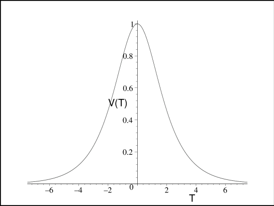
Figure 1: Possible form of the open string tachyon potential $V(T)$ on a SD-brane in Type II a,b superstring theory.

In our analysis we use the potential

$$V(T)=\frac{1}{\cosh\left(T/\sqrt{2}\right)}$$ (4.64)

because it agrees with open string field theory calculations for large values of the tachyon for unstable D-brane systems in Type II a,b superstring theory. It is not known what the exact potential is for intermediate times but our solutions are only mildly affected by its particular form. The expression for the tachyon when $\lambda=0$, i.e., when there are no couplings to the bulk supergravity modes, is

$$T(t)=-\sqrt{2}\;{\rm arcsinh}\left(-\dot{T}(0)\sinh\frac{t}{\sqrt{2}}\right)$$ (4.65)

for the boundary conditions (4.61). When the boundary conditions are of the form (4.63), the analytic expression for the tachyon is

$$T(t)=-\sqrt{2}\;{\rm arcsinh}\left(\sinh\left(-\frac{T(0)}{\sqrt{2}}\right)\cosh\frac{t}{\sqrt{2}}\right).$$ (4.66)

Figure 2 shows a tachyon profile for $T(0)=0.83$ and $\dot{T}(0)=0$. Homogeneous solutions such as eqs. (4.65) and (4.66), derived from a tachyonic action, correspond to a fluid that has a constant energy density and vanishing pressure asymptotically (tachyon matter). We will shortly see how these features are affected by the inclusion of couplings to bulk modes.

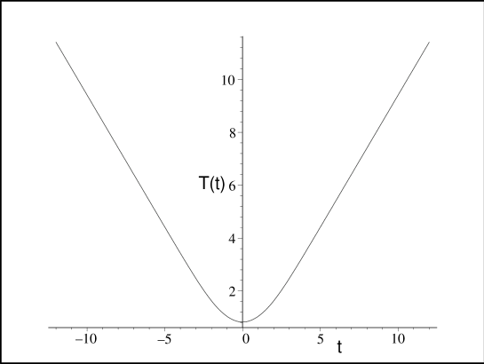
Figure 2: The tachyon field evolution for $\dot{T}(0)=0$ and $T(0)=0.83$.

4.2 R-symmetry group

Before presenting the numerical results we comment on the issue of R-symmetry. As pointed out in ref. [1], SD-brane solutions should be invariant under the transverse Lorentz transformations leaving the location of the brane fixed. This corresponds to an $SO(1,8-p)$ R-symmetry. This property is embodied in the supergravity solutions found in refs. [1, 4, 5] where the transverse space metric has a factor of the form: $R(t)^{2}dH_{8-p}^{2}$. The embedding group of the hyperbolic space $H^{8-p}$ is $SO(1,8-p)$. This explains why we study supergravity solutions with $k_{\parallel}=0$ and $k_{\perp}=-1$ in more details. However, the cases with $k_{\perp}=0$ are also candidate solutions for SD-brane (and, more generally, unstable D-brane) supergravity solutions. We present an analysis of those and other cases in section 4.4.

It is suggested in ref. [1] that the spacelike naked singularities [1, 4, 5] associated with the supergravity SD-branes could be resolved by using a metric ansatz that allows for a breaking of the R-symmetry in the region around the core of the object ($t=0$). The intuition from the AdS/CFT correspondence comes from ref. [36] which describes cases of spontaneously broken R-symmetry. Our ansatz as it is cannot accommodate such an R-symmetry breaking. Presumably, this would correspond to a time-dependent process by which the R-symmetry is broken down to $SO(8-p)$ in a finite region. The closest our ansatz can come to realizing this scenario is if we consider the cases with $k_{\perp}=0$. Then, the transverse symmetry group is $ISO(8-p)$, the compactification of which is $SO(8-p)$. We find that solutions with $k_{\perp}=0$ are regular and asymptotically flat. Moreover, as we will see in section 4.4, a generic feature of the $k_{\perp}=0$ solutions is that the effective string coupling $g_{s}\exp(\Phi(t))$ vanishes asymptotically. We will also remark on the cases with $k_{\perp}$ and/or $k_{\parallel}$ equal to +1, which all develop big-crunch singularities in finite time.

4.3 Numerical SD-brane solutions

Our ansatz for describing supergravity SD$p$-brane solutions is

$$ds^{2}_{Sp} = -dt^{2}+a(t)^{2}d{\vec{y}}^{2}+R(t)^{2}dH_{8-p}^{2},$$

$$C = C(t)\,,\quad\Phi=\Phi(t),$$ (4.67)

where we have taken $k_{\parallel}=0$ and $k_{\perp}=-1$ in accord with the original paper ref. [1]. Again, these supergravity bulk modes will be excited by couplings to an homogeneous open string tachyon as described in section 3.1. We consider only homogeneous solutions (i.e., depending only on time). As discussed earlier, it is possible that inhomogeneities might play an important role in the creation/decay process [33], but we are postponing this issue for now.

The resulting system of coupled differential equations for which we will find solutions is of course highly non-linear. Among other things, this implies that it is not possible to extract scaling behavior for the fields from their equations of motion. We could therefore expect that the behavior of these solutions depends in a physically important way on the initial conditions for the field components involved: $a(t)$, $R(t)$, $C(t)$, $\Phi(t)$ and the source $T(t)$. We will see that the qualitative behavior of the supergravity SD-brane solutions actually does not depend very much on these initial conditions.

The multiplicity of potential solutions could be large: one solution would be expected for each set of initial conditions. Now, for SD-branes the number of solutions is greatly restricted by the constraint equation (3.2). It would appear natural to consider, as candidate solutions for SD-branes, those which are time-reversal symmetric around $t=0$. In fact, precisely time-symmetric solutions actually do not exist! That is, unless they have $k_{\parallel}=0,k_{\perp}=+1$, in which case they have R-symmetry which is markedly in conflict with the proposals of earlier papers, e.g. [1]. As we said above, these solutions with wrong R-symmetry also develop a big-crunch singularity in finite time.

In a sense, motivated by inflationary cosmology, the absence of precisely time-symmetric solutions is not particularly bothersome to us. What we mean by this is that it is an extremely fine-tuned situation to have exactly zero kinetic energy in each of the bulk fields at $t=0$. Any small quantum fluctuation of a bulk field takes us away from time-symmetry. Therefore, all solutions which we will exhibit here will have some kinetic energy in one or more of the bulk fields at $t=0$. And the kick in bulk field(s) at $t=0$, required to solve the initial constraint, can actually be made very small by, e.g., choosing $R(0)$ large. Such initial conditions are quite generic: even a little bit of kick in $a(t)$ alone will suffice to give completely nonsingular solutions for the entire time-evolution. The precisely time-symmetric solutions are however inaccessible; see subsection 4.4.2 for a more detailed exposition of this case.

Another reason why we find a slight bulk asymmetry at $t=0$ reasonable relates to particle/string production. We have of course neglected such production in our analysis. It is nonetheless clear that, for a full SD-brane solution, backreaction will combine with particle production to make bulk fields naturally asymmetric. It is only in the approximation of zero backreaction that time-symmetry is possible when particle production occurs, but of course that approximation cannot be self-consistent.

Let us now move to the solution of our problem of interest. Unfortunately we have been unsuccessful at finding analytical expressions for the bulk modes and tachyon field when their mutual coupling is non-vanishing ($\lambda\neq 0$). We therefore resorted to solving the corresponding system of differential equations numerically. In what follows we show the results associated with a SD4-brane, and present some interesting analysis of the effect of varying the initial conditions. We provide general comments for other SD-branes with $p<7$ and explain how the SD$p$-branes with $p=7,8$ are different. We comment on the robustness of the solutions to changes in initial conditions. Throughout our analysis we pay special attention to the impact of varying the initial condition $\Phi(0)$ on the dilaton, because this controls the string coupling close to the hilltop.

For finding the numerical solutions we fix the initial conditions at $t=0$, and evolve this data forward in time. Then, we evolve the same data backward in time from $t=0$. The result is the solution associated with a full SD-brane, i.e., the bulk fields sourced by the open string tachyon as it evolves from $t=-\infty$ to $t=+\infty$. In this section we present the results associated with a SD4-brane with boundary conditions

$$T(0)=0.83\,,\;\;\;\dot{T}(0)=0\,,\;\;\;a(0)=1\,,\;\;\;\dot{a}(0)=0.091\,,\;\;\;R(0)=10\,,$$

$$\dot{R}(0)=0.01\,,\;\;\;\phi(0)=-1\,,\;\;\;\dot{\phi}(0)=0.01\,,\;\;\;C(0)=0\,,\;\;\;\dot{C}(0)=0.01\,,$$ (4.68)

and $\lambda=0.1\,$. Again, these solutions correspond to the tachyon rolling up the potential from $T=+\infty$ ($t=-\infty$) and coming to a halt for $T(0)=0.83$ which corresponds to a turning point. Then, the tachyon evolves toward the bottom of the potential at $T=+\infty$ for $t=+\infty$. This type of tachyon evolution was considered, for example, in refs. [14, 10] where they are called full S-branes. We could of course have chosen different initial conditions - including some with less time-asymmetry; these are used just for the sake of illustration.

4.3.1 Deformation of the tachyon field

Figure 2 shows the evolution of the tachyon for the S4-brane. For $\lambda=0$ (no coupling between the closed and the open string modes), we find

$$\lim_{t\rightarrow\pm\infty}T(t)=\pm t.$$ (4.69)

This observation is suggestive that the tachyon field might play the role of time itself in cosmological models driven by brane decay (as proposed in ref. [29]). We find that this asymptotic behavior for the tachyon survives when couplings to bulk modes are introduced. In fact, for $\lambda\neq 0$ we find

$$\lim_{t\rightarrow\pm\infty}T(t)=\pm(t+\kappa_{\scriptscriptstyle\pm T}).$$ (4.70)

The constants $\kappa_{\scriptscriptstyle\pm T}$ depend non-trivially on the boundary conditions at $t=0$ and $p$. For example, as $p$ is increased $\kappa_{\scriptscriptstyle T}$ decreases. Also, for large values of $\Phi(0)$ the tachyon deformation from the flat space case becomes larger. As mentioned in Appendix B, for $\lambda=0$ the state of the tachyon for large time ($t\rightarrow\pm\infty$) is that of a perfect fluid with constant energy density and vanishing pressure. This is the so-called tachyon matter. We find that for $\lambda\neq 0$, both the energy density and the pressure (physical quantities measured in the Einstein frame) vanish. In other words, the tachyon matter is clearly only an illusion of the $g_{s}\rightarrow 0$ limit.

We consider briefly the effect of varying the initial conditions $\dot{T}(0)$ and $T(0)$. For half SD-branes (i.e., the future of the full SD-branes) we find that the time it takes the tachyon to reach the bottom of its potential increases for smaller values of $\dot{T}(0)$ and $T(0)$. Not only that, for very small initial velocities the tachyon stays perched at the top of the potential for a certain period of time. In general, we observe that it takes less time for the tachyon to reach the bottom of its potential when we increase $\lambda$. Now, we also observe that the difference between the curves associated with flat space ($\lambda=0$) and $\lambda\neq 0$ tachyons decreases as $\dot{T}(0)$ and $T(0)$ increase. Also, for large negative values of $\Phi(0)$, $\kappa_{\scriptscriptstyle T}$ becomes very small. This is simply a reflection of the fact that such cases correspond to a very small initial string coupling (see below for details).

There is another interesting feature of the tachyon when coupled to the massless closed string modes. Firstly, the time it takes the tachyon to reach the bottom of its potential is not significantly altered even when considering large values of the ‘coupling’ $\lambda$. Finally, we find that as the coupling $\lambda$ is increased, $\kappa_{\scriptscriptstyle T}$, or the deformation away from the flat space tachyon, increases correspondingly.

4.3.2 Time-dependent string coupling

The string coupling is given by the expression

$$g_{s}=e^{<\Phi_{0}>}\,,$$ (4.71)

where $\Phi_{0}$ is the background dilaton field in the absence of sources, i.e., strings and D-branes. Typically the presence of stringy excitations will modify the coupling of the theory,

$$g_{s}\rightarrow g_{s}e^{\Phi(\eta)},$$ (4.72)

where $\eta$ is a spacelike variable for D-branes and is timelike for SD-branes.

For supergravity D$p$-brane solutions the dilaton field is (see, for example, ref. [37]),

$$g_{s}(r)=g_{s}e^{\Phi(r)}=g_{s}\left(1+\frac{c_{p}g_{s}N_{p}l_{s}^{7-p}}{r^{7-p}}\right)^{\frac{1}{4}(3-p)},$$ (4.73)

where $c_{p}=(2\sqrt{\pi})^{5-p}\Gamma[\frac{1}{2}(7-p)]$. The string coupling is seen to vary according to whether test closed strings propagate close or far from the horizon ($r=0$) of these geometries. For all static supergravity solutions (including NS5-branes), the asymptotic string coupling is such that

$$\lim_{r\rightarrow+\infty}g_{s}(r)=g_{s}.$$ (4.74)

The effect of supergravity D-branes is therefore to modify the coupling locally. For $p<3$, it is large close to the horizon and decreases to $g_{s}$ as $r\rightarrow+\infty$. For $p>3$, the string coupling is small close to the horizon but increases to $g_{s}$ for large $r$. The case $p=3$ is special because the dilaton field sourced by the 3-brane is constant throughout the spacetime. Typically, the size of the region where the dilaton is not constant depends on the parameter $g_{s}N$. Large values of this parameter are associated with larger regions where dilaton perturbations associated with the brane are noticeable.

The solutions associated with supergravity SD-branes induce dilaton perturbations corresponding to a time-dependent string coupling,

$$g_{s}(t)=g_{s}e^{\Phi(t)}.$$ (4.75)

We find that the time dependence of the dilaton sourced by SD-branes is qualitatively different when compared to the radial dependence of the dilaton associated with regular D-branes.

Figure 3 shows the time-evolution of the dilaton function $g_{s}^{-1}e^{\Phi(t)}$ for a SD4-brane with boundary conditions (4.3). Typically, the function $g_{s}^{-1}e^{\Phi}(t)$ decreases from $t=0$ as $t\rightarrow\pm\infty$. We find that smaller values of $p$ correspond to larger asymptotic string couplings.

The dilaton field generated by SD-branes has at least two interesting properties. First, all solutions are such that the dilaton stabilizes to a constant asymptotically,

$$\lim_{t\rightarrow\pm\infty}\Phi(t)=\Phi_{\pm\infty}.$$ (4.76)

More generally, the relation between $\Phi_{+\infty}$ and $\Phi_{-\infty}$ depends on the initial conditions. This last statement applies to all other bulk fields. Secondly, the asymptotic value of the dilaton is always smaller than its initial value at $t=0$,

$$\Phi_{\pm\infty}<\Phi(0).$$ (4.77)

This implies that the late/early string coupling ($t\rightarrow\pm\infty$) is always smaller than the coupling when the tachyon is at the top of its potential ($t=0$), i.e.,

$$g_{s}e^{\Phi_{\pm\infty}}<g_{s}e^{\Phi(0)}.$$ (4.78)

We find that the qualitative features shown on figure 3 are preserved when the boundary conditions on the various fields are changed. Nevertheless, we consider the effect of varying $\Phi(0)$ in some detail. An interesting quantity to study is the ratio

$$h=\frac{e^{\Phi_{\pm\infty}}}{e^{\Phi(0)}},$$ (4.79)

which gives a quantitative measure of how much the initial string coupling is modified asymptotically. The tachyon profile is not altered significantly when the initial condition on $\Phi(t)$ is varied. Nevertheless, we observe that that for large values of $\Phi(0)$ (large initial coupling) the tachyon field reaches the bottom of the potential well faster. A large initial coupling also means that the bulk fields relax faster to their stable asymptotic configuration compared to cases where $\Phi(0)$ is smaller. The overall effect on the bulk fields is also enhanced for larger values of $\Phi(0)$. For example, as the initial coupling is increased the scale factor $a(t)$ stabilizes to significantly smaller values (see next section). As for the dilaton field itself, we find that the ratio $h$ is large for larger values of $\Phi(0)$. For very small values of the initial string coupling (large negative values of $\Phi(0)$), the ratio $h$ approaches unity.

In summary, we find that the parameter $\Phi(0)$, i.e., the parameter determining the string coupling when the tachyon is close to the top of its potential, strongly determines the importance of the unstable brane source effect on the supergravity bulk modes.

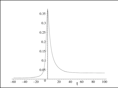
Figure 3: Time dependence of the function $e^{\Phi(t)}/g_{s}$ for a SD4-brane with boundary conditions (4.3).

4.3.3 Gravitational field

We now describe the effect of the unstable brane source on the time-dependent metric components $a(t)$ and $R(t)$.

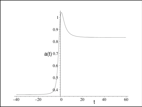
Figure 4: The scale factor on the worldvolume of a supergravity SD4-brane with boundary conditions (4.3).

Figure 4 shows the scale factor $a(t)$ on the worldvolume of a SD4-brane with the boundary conditions (4.3). A general feature is that away from $t=0$ the scale factor monotonically decreases from its initial value, $a(0)$, to a stable asymptotic value,

$$\lim_{t\rightarrow\pm\infty}a(t)=a_{\pm\infty},$$ (4.80)

with $a_{+\infty}>a_{-\infty}$. The time it takes for this scale factor to reach its asymptotic value corresponds roughly to the time it takes for the tachyon to reach the bottom of its potential. As pointed out above, for large initial values of the dilaton, $\Phi(0)$, the asymptotic values of the scale factor, $a_{\pm\infty}$, become smaller. Correspondingly, when the initial coupling is weak the effect of the probe on the bulk modes is small and $a(t)$ stabilizes to a value closer to its initial value $a(0)$.

Figure 5 shows the behavior of the metric function $R(t)$. A generic feature of the supergravity SD-brane solutions is that

$$\lim_{t\rightarrow\pm\infty}R(t)=\pm(t+\kappa_{\scriptscriptstyle\pm R}).$$ (4.81)

The constants $\kappa_{\scriptscriptstyle\pm R}$ are generically larger for larger values of $p$.

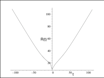
Figure 5: The SD4-brane transverse scale factor $R(t)$ with boundary conditions (4.3).

4.3.4 Ramond-Ramond field

Figure 6 shows the time dependence of the Ramond-Ramond form field for a supergravity SD4-brane with boundary conditions (4.3). Again, the energy stored in this field (proportional to its time-derivative) goes to zero in approximately the time it takes for the tachyon to reach the bottom of its potential. A generic feature of the Ramond-Ramond field associated with a SD-brane is therefore,

$$\lim_{t\rightarrow\pm\infty}C(t)=C_{\pm\infty},$$ (4.82)

where $C_{\pm\infty}$ is a constant. Typically we find that these constants are smaller for larger values of $p$.

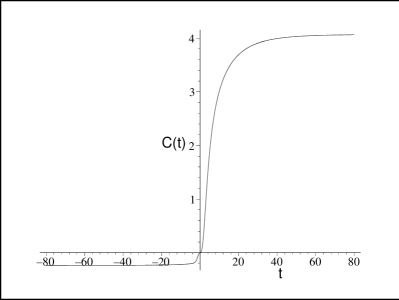
Figure 6: The SD4-brane Ramond-Ramond field $C(t)$ associated with the boundary conditions (4.3).

4.3.5 Curvature bounds and asymptotic flatness

The supergravity equations of motion are derived from a worldsheet calculation by requiring that, at a certain order in perturbation theory, the beta-functions associated with bulk fields vanish. Typically, there are higher order (in $\alpha^{\prime}$) curvature corrections to the beta-functions. These corrections are negligible only if the curvature involved is small when measured with respect to the string length, $l_{s}=\sqrt{\alpha^{\prime}}$. This is why our solutions can, strictly speaking, be trusted only if the curvature involved is such that $\left|{\cal R}\right|,\;\left|{\cal R}_{\mu\nu}{\cal R}^{\mu\nu}\right|,\;\left|{\cal R}_{\mu\nu\rho\lambda}{\cal R}^{\mu\nu\rho\lambda}\right|$ are small. We verify that this condition is satisfied by studying the behavior of the time-dependent Ricci scalar of the supergravity SD-branes,

$${\cal R}(t)= 2(p+1)\frac{\ddot{a}}{a}+2(8-p)\frac{\ddot{R}}{R}+2(p+1)(8-p)\frac{\dot{a}}{a}\frac{\dot{R}}{R}$$ (4.83)

$$+p(p+1)\left(\frac{\dot{a}^{2}}{a^{2}}+{\frac{k_{\parallel}}{a^{2}}}\right)+(8-p)(7-p)\left(\frac{\dot{R}^{2}}{R^{2}}+\frac{k_{\perp}}{R^{2}}\right),$$

where $k_{\perp}=-1$ and $k_{\parallel}=0$ for the cases of interest here.

A property of the solutions, which is apparent from studying the evolution of bulk modes, is that of asymptotic flatness. In fact, we find

$$\lim_{t\rightarrow\pm\infty}ds^{2}_{Sp}=-dt^{2}+a_{\pm\infty}^{2}d{\vec{y}}^{2}+(t+\kappa_{\pm R})^{2}dH_{8-p}^{2}\,,$$ (4.84)

$$\lim_{t\rightarrow\pm\infty}\Phi(t)=\Phi_{\pm\infty},\;\;\;\;\lim_{t\rightarrow\pm\infty}C(t)=C_{\pm\infty},$$ (4.85)

where $a_{\pm\infty}$, $\kappa_{\pm R}$, $\Phi_{\pm\infty}$ and $C_{\pm\infty}$ are constants. Both the first- and second-derivative of the bulk modes vanish asymptotically. The resulting brane configuration is then clearly flat for $t\rightarrow\pm\infty$, as it should be.

An important question to answer at this stage is: Which quantity in the problem sets an upper bound on the curvature for SD-branes ? First, we have found that whatever the curvature is at $t=0$, its absolute value will never exceed it significantly in the course of the evolution. This is true only for half S-branes with boundary conditions corresponding to positive derivatives of the bulk fields. More generally for full S-branes the acceptable solutions are those with a combination of the boundary conditions such that

$$\lim_{t\rightarrow 0}\left|{\cal R}(t)\right|\ {\rm{small}}\ .$$ (4.86)

These requirements are certainly attainable within the self-consistent supergravity approximation we are considering — along with the specific ansatz we introduced in order to be able to solve the equations numerically.

4.3.6 The $p=7$ and space-filling SD-branes

The case $p=8$ should be special because there is no transverse space into which “energy” can be dissipated. The only bulk fields involved are then the metric component, $a(t)$, the dilaton, $\Phi(t)$, and the Ramond-Ramond field, $C(t)$. We find that the time-derivative of the scale factor, $\dot{a}(t)$, decreases to zero, as $t\rightarrow\pm\infty$, many orders of magnitude slower than for $p<7$. The scale factor $a(t)$ also goes to zero after an infinite time (see section 4.3.7 for a physical interpretation) which is to be contrasted with the cases $p<7$ where $a_{\pm\infty}\neq 0$. One would expect that to be the source of a curvature singularity at $t=\pm\infty$ but it is not the case. The Ricci scalar for the space filling SD-brane is

$${\cal R}(t)=-72\left(\frac{\dot{a}}{a}\right)^{2}-\frac{9}{2}\left(\frac{e^{\Phi}\dot{C}}{a^{9}}\right)^{2}+36\dot{\Phi}\frac{\dot{a}}{a}+\frac{9}{2}\lambda e^{\Phi}\Delta^{1/2}V(T).$$ (4.87)

Curvature singularities are avoided because all time-derivatives in the problem go to zero faster than the scale factor as $t\rightarrow\pm\infty$. In particular, the quantity $e^{\Phi}\dot{C}$ goes to zero faster than $a(t)$ for large time. Also the string coupling slowly goes to zero asymptotically ($\Phi_{\pm\infty}\rightarrow-\infty$)! For the Ramond-Ramond field we find the same behavior as for the cases $p<7$. The only difference is that the relaxation time of the bulk modes is many orders of magnitude larger than in the other cases.

The functions $a(t)$, $\Phi(t)$ and $C(t)$ associated with the SD7-brane behave in the same way as the space-filling SD-brane. Of course in this case there is a transverse space and we find that the relaxation of $\left|R(t)\right|$ to its asymptotic form $t+\kappa_{\scriptscriptstyle\pm R}$ takes an infinite amount of time. In other words, it relaxes to its asymptotic form much slower than for the cases $p<7$.

4.3.7 Einstein frame

Let us end this section with a remark about the physics of our SD-branes in Einstein frame. This would be the more natural and more physical frame to use in discussions of potential uses of rolling tachyons in the context of cosmology.

The transformation from string frame to Einstein frame involves a multiplicative factor of $e^{-\Phi/2}$ for $d=10$, which is the dimension in which we are working here. Now, we have already commented at length on the behavior of the time-dependent dilaton field in section 4.3.2. The essential physics there was that the dilaton is biggest at the top of the potential hill; in particular, it stabilizes in the infinite past and future at a constant value smaller than the initial condition at the hilltop. Dilaton derivatives also remain small at all times during the evolution. Therefore, most of the qualitative features of our solutions will be preserved upon transformation to Einstein frame; in particular, all solutions remain completely nonsingular.

A case that deserves further comments is that of the space filling SD8-brane discussed earlier. In string frame the metric is written

$$ds^{2}_{S8}=-dt^{2}+a(t)^{2}d{\vec{y}}^{2}.$$ (4.88)

Upon converting to Einstein frame we get the metric

$$ds_{ES8}^{2}=-d\tau^{2}+a_{E}(\tau)^{2}d{\vec{y}}^{2},$$ (4.89)

where we have used a change of coordinate such that $d\tau^{2}=e^{-\Phi/2}dt^{2}$, and where

$$a_{E}(\tau)=e^{-\Phi(t)/4}a(t).$$ (4.90)

For the SD8-brane we found

$$\lim_{t\rightarrow\pm\infty}a(t)=0\,,\;\;\;\;\lim_{t\rightarrow\pm\infty}e^{\Phi(t)}=0.$$ (4.91)

In string frame this implies that the metric “closes off” at infinity but in the (more physical) Einstein frame the converse happens, i.e., the limit $\tau\rightarrow\pm\infty$ corresponds to a constant scale factor,

$$\lim_{t\rightarrow\pm\infty}a_{E}(\tau)={\rm const.}$$ (4.92)

This is a very sensible result. We mentioned before that, because of the absence of a transverse space, there appeared to be no channel into which the energy could go. We therefore find that asymptotically the energy has gone into inflating the worldvolume of the SD-brane. In fact, the relaxation time for the gravitational field is essentially infinite.

4.4 Other classes of solutions

In this section we present a more general analysis of the family of solutions with parameters $\{k_{\parallel},k_{\perp}\}$ associated with the metric ansatz (3.36).

4.4.1 Comment about the numerical analysis

For $\lambda=0$ there is clearly no source for the the bulk fields. The equation of motion for the tachyon is then (B.131). In Appendix B we found analytic expressions for the corresponding solutions. They have the large time property

$$\frac{V(T)}{\sqrt{\Delta}}={\rm const.}$$ (4.93)

However, if we solve eq. (B.131) numerically (using the same techniques as in section 4) we find that $V(T)/\sqrt{\Delta}$ appears to become constant but, after some more time has elapsed, its behavior becomes erratic, i.e., it starts oscillating with increasingly large amplitudes. Clearly this is only an artifact of the numerical analysis. The tachyon evolution is such that

$$\lim_{t\rightarrow\pm\infty}V(T)=0,\;\;\;\lim_{t\rightarrow\pm\infty}\sqrt{\Delta}=0.$$ (4.94)

The source of the problem can be traced down to the numerics having difficulties to evaluate a $\frac{0}{0}$ division at large times.

The same thing happens for $\lambda\neq 0$. The quantity that becomes ambiguous for large time is then

$$\frac{e^{\Phi(t)}V(T)}{\sqrt{\Delta}}.$$ (4.95)

Again, the problem is associated with the fact that both $e^{\Phi(t)}\,V(T)$ and $\sqrt{\Delta}$ are zero for large time. It is important to resolve this ambiguity because the quantity (4.95) directly feeds in the equations of motions for the bulk fields. We are able to show numerically that (at least for the solutions considered in this work) for large time

$$\frac{e^{\Phi(t)}V(T)}{\sqrt{\Delta}}=0.$$ (4.96)

Similarly to the $\lambda=0$ case, past some finite time the behavior of the function (4.95) becomes erratic. To obtain numerical solutions representing the evolution for all times we did the following: past the time value where (4.95) becomes ill-behaved, we solve the system of differential equations without a source, i.e., for

$$\frac{e^{\Phi(t)}V(T)}{\sqrt{\Delta}}=0,\;\;\;e^{\Phi(t)}V(T)\sqrt{\Delta}=0,$$ (4.97)

and appropriate boundary conditions. This introduces negligible errors.

4.4.2 Time-reversal symmetric solutions

We consider the time-reversal symmetric solutions, i.e., those associated with bulk fields having vanishing time-derivatives at $t=0$:

$$\dot{a}(0)=\dot{R}(0)=\dot{C}(0)=\dot{\Phi}(0)=0.$$ (4.98)

The constraint equation (3.2) at $t=0$ is then

$$\frac{V(T)}{\sqrt{\Delta}}=\frac{1}{\lambda e^{\Phi}}\left(p(p+1)\frac{k_{\parallel}}{a^{2}}+(7-p)(8-p)\frac{k_{\perp}}{R^{2}}\right).$$ (4.99)

The LHS being positive-definite, the constraint can be satisfied if and only if the metric ansatz contains a subspace of positive curvature. These consist in five categories of solutions, i.e., $\{k_{\parallel},k_{\perp}\}=\{0,1\},\{-1,1\},\{1,-1\},\{1,1\},\{1,0\}$. We have performed a detailed analysis of these solutions for $p=4$ and $\dot{T}(0)\leq 1/10$. Typically, we find that when the tachyon has reached a point of its evolution where $|V(T)|\simeq 0$, labelled $t_{c}$, the solutions develop a curvature singularity. The behavior of the bulk fields is as follows. The time derivative of the scale factor is such that

$$\lim_{t\rightarrow t_{c}}\dot{a}=-\infty,\;\;\;\lim_{t\rightarrow t_{c}}a(t)=0,$$ (4.100)

which corresponds to a big-crunch singularity on the ($p+1$)-dimensional worldvolume. The cases $\{k_{\parallel}=-1,k_{\perp}=1\}$, $\{k_{\parallel}=0,k_{\perp}=1\}$ and $\{k_{\parallel}=1,k_{\perp}=0\}$ are such that

$$\lim_{t\rightarrow t_{c}}\dot{R}(t)=-\infty,\;\;\;\lim_{t\rightarrow t_{c}}R(t)=0,$$ (4.101)

corresponding to the transverse spherical space collapsing to zero-size in finite time. For $\{k_{\parallel}=1,k_{\perp}=1\}$ and $\{k_{\parallel}=1,k_{\perp}=-1\}$, we find

$$\lim_{t\rightarrow t_{c}}\dot{R}(t)=+\infty,\;\;\;\lim_{t\rightarrow t_{c}}R(t)=+\infty.$$ (4.102)

For $k_{\perp}=-1$, $R(t)$ goes to infinity faster than $t$. All solutions are such that

$$\lim_{t\rightarrow t_{c}}\dot{\Phi}(t)=-\infty.$$ (4.103)

Generically, the large time behavior of the R-R field is well-behaved, i.e.,

$$\lim_{t\rightarrow t_{c}}\dot{C}(t)\approx 0,\;\;\;\lim_{t\rightarrow t_{c}}C(t)=C_{c},$$ (4.104)

where $C_{c}$ is finite but typically many orders of magnitudes larger than the constants $C_{\infty}$ associated with the regular solutions presented earlier. The case $\{k_{\parallel}=0,k_{\perp}=-1\}$ is special because then the time derivative of the R-R field diverges as well at finite time.

We believe our conclusions to be unaltered for other values of $p$. We found no evidence that the singularities are resolved when the time-reversal symmetry is broken.

4.4.3 More regular solutions

Another class of candidate SD-brane solutions we have studied are those with $k_{\parallel}=0$ and $k_{\perp}=0$. The results we present for these solutions are generic, i.e., they hold for all $p$ and reasonable boundary conditions (i.e., first derivatives not too large). Firstly, the solutions are always asymmetric around $t=0$ since it was shown before that, for consistency, at least one of the bulk fields must have non-vanishing kinetic energy at $t=0$. The level of asymmetry will be reduced by having smaller derivatives of the bulk fields at $t=0$. The corresponding solutions are regular and asymptotically flat. We find that

$$\lim_{t\rightarrow\pm\infty}\dot{a}(t)=0,\;\;\;\lim_{t\rightarrow\pm\infty}a(t)=0,$$ (4.105)

and

$$\lim_{t\rightarrow\pm\infty}\dot{R}(t)=0,\;\;\;\lim_{t\rightarrow\pm\infty}R(t)={\rm const.}$$ (4.106)

In Einstein frame both scale factors asymptote to non-zero constants. For the dilaton we obtain

$$\lim_{t\rightarrow\pm\infty}\dot{\Phi}(t)=0,\;\;\;\lim_{t\rightarrow\pm\infty}\Phi(t)=-\infty,$$ (4.107)

i.e., the string coupling vanishes asymptotically. Finally the R-R field behaves like

$$\lim_{t\rightarrow\pm\infty}\dot{C}(t)=0,\;\;\;\lim_{t\rightarrow\pm\infty}C(t)={\rm const.}$$ (4.108)

We note that the relaxation time for these solutions is many orders of magnitude larger than for the $\{k_{\parallel}=0$, $k_{\perp}=-1\}$ cases presented earlier.

The two remaining cases are $\{k_{\parallel},k_{\perp}\}$ equal to $\{-1,-1\}$ and $\{-1,0\}$. We found evidence that the corresponding solutions are regular and asymptotically flat.

5 Discussion

Our primary motivation for this work was the general problem of seeking mechanisms for resolution of singularities in spacetimes of interest in string theory. SD-brane supergravity spacetimes presented in refs. [1, 4, 5] create somewhat of a supergravity emergency because they are not only singular but nakedly so.

An important first step in the resolution program was made in ref. [7], where some effects of unstable brane probes in these backgrounds were considered. In particular, the probe physics was also sick, and taking this analysis seriously led to an even more dire assessment of the likelihood of singularity resolution without resorting to the inclusion of massive string modes in both the open and closed sectors. In our work, then, we began by plumbing the depths of the probe approach. We found it to be generally insufficient for our purposes; one reason is that the probe approximation takes itself out of its regime of self-consistency.

We then launched into an investigation of the physics of the gravitational fields exerted by SD$p$-branes for general $p$ by including backreaction. In order to get started on this problem, we had to make the approximation of considering only the most relevant open- and closed- string modes, with full gravitational backreaction taken into account. The equations we derived are highly nonlinear and couple brane with bulk, so did not lend themselves to solution analytically. We therefore resorted to numerical techniques to search for solutions. Because of this restriction, we had to use an ansatz which smeared the branes in the transverse space; this allowed us to turn the equations into ODE’s and integrate them numerically. An essential step was to begin the numerical integration near the top of the potential hill, and then reconstruct asymptopia, which we were able to do successfully. Generically, the solutions are time-reversal asymmetric. We have shown that the time-reversal symmetric solutions with the correct R-symmetry are unavailable. Given our two-stage approximation (lowest modes, and smeared ansatz), we found it rather satisfying that significant progress in the resolution program is already found at this level. In particular, our solutions for rolling tachyons backreacting on spacetime are completely nonsingular, and our approximations satisfy the fundamental property of self-consistency. We find these conclusions suggestive of resolution of the SD-brane spacetime singularity emergency.

It is however hard to know for sure whether our nonsingular results will survive refinement. Therefore, let us now make some specific remarks about technical roadblocks we encountered which forced us to make approximations, their physical consequences, and future outlook.

Section 3.1 was where we derived the coupled tachyon-supergravity equations for a general brane distribution, assuming Chern-Simons terms are turned off in a consistent truncation. Our resulting equations are on the one hand remarkably non-robust, and on the other quite robust. What we mean by non-robustness is this: our ability to obtain nonsingular evolution depends importantly on the structure of these equations of motion. Signs are crucial, coefficients are crucial, and so is the inclusion of Ramond-Ramond fields. In other words, our nonsingular results are highly specific to the field couplings arising from the low-energy approximation to string theory. Other “S-branes” arising from “string-motivated” actions will probably not possess similarly nonsingular behavior. The positive type of robustness we refer to is also a desirable property. What we see manifestly is that the precise form of the potentials $\{V(T),f(T)\}$ is not important, apart from the large-$|T|$ behavior which had been derived elsewhere. The most obvious refinement of our work here will be to attack the problem of relaxing the requirement of zero NS-NS $B$-field. Allowing $B^{(2)}$ to be turned on will allow us to break $ISO(p{+}1)$ on the worldvolume and allow inhomogeneous tachyonic modes — the importance of which is discussed in refs. [17, 33] — and also to turn on more components of R-R fields. Inhomogeneities would of course have to be included in initial conditions, because homogeneous on-shell tachyons do not couple to non-homogeneous tachyons [32]. We have postponed the non-homogeneous problem to the future mainly because it is messy; our work reported here should be considered a step in a larger program.

The other important approximation we made in our work was in section 3.2, where we had to smear the SD-brane sources in the transverse space to facilitate integrating the equations numerically by turning them into ODE’s. This limits our ability to fully probe the properties of the system in which we are interested. Here we would also like to record another physical consequence of this ansatz. Namely, this restriction has notable, negative, consequences for our ability to track whether black holes form as intermediate states during the time evolution of our coupled system including full backreaction. The issue of black holes was raised in the discussion section of ref. [5]. The essential point is that a black hole intermediate state may arise as an alternative to SD-brane formation and decay, at least with the half-advanced, half-retarded propagator. The fine-tuned nature of the initial conditions producing SD-branes highlights a reason why integrating partial differential equations of motion (including dependence on transverse coordinates) may be particularly difficult numerically. Or the obstruction to finding the full solution may yet turn out to be negotiable. It will also be interesting to think further about particle/string production.

Let us end with some somewhat speculative remarks. Typically in the limit $g_{s}N\rightarrow 0$ the open and closed strings decouple. This is true in our effective lowest-modes analysis here, but also explicit in other worldsheet-inspired approaches. There should also exist a limit (in time) to be taken where only the open strings survive. From the worldsheet definition of a SD-brane, it is suggestive that the open string degrees of freedom would combine to form a Euclidean conformal field theory in $p+1$ dimensions. The same appears true when considering the effective action of massless open string degrees of freedom on an unstable D-brane [34]. In both approaches, however, it is not clear what the role of the tachyon could be. Physically, it is the source of a process by which energy is siphoned out of the open string sector and pumped into the closed string sector. So, in a sense, the decay of a D-brane through tachyon condensation corresponds to the decrease of a $c$-function-like quantity on the gauge theory side. Then, we can entertain the idea that time-evolution on the gravity side should really be regarded as a renormalization group (RG) flow on the gauge theory side. From this viewpoint, formation and decay of a SD-brane would be a process corresponding to first an inverse RG flow (integrating in degrees of freedom) followed by regular RG flow (integrating out degrees of freedom). This might be related to the study of open string tachyon condensation using RG flow in the worldsheet theory [40].

Appendix A Regular KMP SD-brane solutions

Among the supergravity solutions found by [5], there exist some that are regular on the horizon located at $t=\omega$. This is only realized for the following values of the parameters,

$$\tilde{k}=2,\;\;\;H=\frac{4}{7-p},\;\;\;G=k_{i}=0.$$ (A.109)

The corresponding metric is

$$ds^{2}= F(t)^{1/2}\alpha(t)^{4/(7-p)}\left(-dt^{2}+t^{2}dH_{8-p}^{2}\right)$$ (A.110)

$$+F(t)^{-1/2}\left[\sum_{i=2}^{p+1}\left(dx^{i}\right)^{2}+\left(\frac{\beta(t)}{\alpha(t)}\right)^{2}\left(dx^{1}\right)^{2}\right].$$

Because these solutions are anisotropic in the worldvolume directions, it is not clear that they are physically relevant. We will nevertheless study some interesting properties not considered in ref. [5]. For example, the region $t=+\omega$ does not correspond to an horizon as suggested by the fact that none of the metric components either vanish or diverge there. For $p$ odd the solutions are time-reversal symmetric so the region $t=-\omega$ is also not an horizon.

A.1 The region close to the origin

For the anisotropic solutions there is no curvature singularity at $t=\omega$. It is therefore interesting to consider the behavior of the metric components and curvature invariants close to the potentially problematic region around the origin, $t=0$. We evaluated the curvature invariants: ${\cal R}$, ${\cal R}_{\mu\nu}{\cal R}^{\mu\nu}$, and ${\cal R}_{\mu\nu\rho\lambda}{\cal R}^{\mu\nu\rho\lambda}$. They identically vanish for $t=0$. The metric tensor there appears suspicious (for example, the component $g_{tt}$ diverges) but we find

$$\lim_{t\rightarrow 0}ds^{2}=-d\tau^{2}+\tau^{2}dH_{8-p}^{2}+\sum_{i=1}^{p+1}\left(dx^{i}\right)^{2},$$ (A.111)

where $\tau=\omega^{2}/t$. The expression (A.111) is simply flat space with part of it written in Milne coordinates. Not surprisingly, we find

$$\lim_{t\rightarrow 0}\dot{\Phi}(t)=0,\;\;\;\;\lim_{t\rightarrow 0}\dot{C}(t)=0,$$ (A.112)

which implies that all stress-energy components vanish in the the region close to the origin.

A.2 Horizon physics

We demonstrate that, contrary to previous claims, many of the anisotropic solutions are actually regular in the full range: $-\infty<t<+\infty$. The anisotropic solutions were already shown to be non-singular at $t=\omega$ and $t=0$. We now investigate the region $t=-\omega$ further. Let us introduce the change of coordinates

$$T=\left(1+\left(\frac{\omega}{t}\right)^{7-p}\right)^{2/(7-p)}t$$ (A.113)

in order to make comparison with the results of ref. [5] easier. For $p$ even, $T=0$ corresponds to $t=-\omega$ while for $p$ odd we have $T=-2\omega$ when $t=-\omega$. A comment in ref. [5] is that $T=0$ corresponds to a (non-naked) curvature singularity. Actually, this is not always the case! For example, we considered the case $p=1$ and computed the associated curvature invariants at all times. Figure 7 shows the evolution of the Ricci scalar for the solution with $\omega=1$ and $\theta=\pi/4$. Clearly, the $p=1$ solution is symmetric under time-reversal and therefore has no curvature singularity. It also does not possess any horizon, a feature common to the regular solutions found in this paper. The qualitative behavior of all curvature invariants is similar to the Ricci scalar and is quite generic, i.e., it is unchanged for all odd values of $p$, $\theta$ and $\omega$. For $p=1$ we obtain

$$\lim_{t\rightarrow\pm\omega}{\cal R}=-\frac{32^{1/3}}{\omega^{2}}\frac{19\cos^{4}\theta-26\cos^{2}\theta+7}{\sin^{5}\theta}.$$ (A.114)

This is finite except for $\theta=0$ in which case the Ricci scalar diverges like $R\sim 1/(t-\omega)^{3}$. We also found expressions for two other curvature invariants (for $p=1$),

$$\lim_{t\rightarrow\pm\omega}{\cal R}_{\mu\nu}{\cal R}^{\mu\nu}=\frac{92^{3/4}}{2\omega^{4}}\frac{-272\cos^{6}\theta+14+255\cos^{4}\theta+101\cos^{8}\theta-98\cos^{2}\theta}{\sin^{10}\theta},$$ (A.115)

$$\lim_{t\rightarrow\pm\omega}{\cal R}_{\mu\nu\rho\sigma}{\cal R}^{\mu\nu\rho\sigma}=\frac{32^{2/3}}{4\omega^{4}}\frac{-112\cos\theta+28+892\cos^{8}\theta-1840\cos^{6}\theta+1032\cos^{8}\theta}{\sin^{10}\theta}.$$ (A.116)

We found expressions with similar qualitative behavior for other values of $p$ odd.

For $p$ even the solutions are not time-reversal symmetric. As pointed out previously, curvature invariants are finite at $t=\omega$ but there is a curvature singularity at $t=-\omega$. These are the spacelike curvature singularities (protected by an horizon at $t=0$) described in ref. [5].

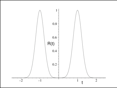
Figure 7: This figure illustrates the Ricci scalar for the $p=1$ anisotropic SD-brane solution with $\omega=1$ and $\theta=\pi/4$. The other curvature invariants behave similarly.

A.3 Unstable brane probe analysis

As mentioned in section 2.2, the motivation behind considering an unstable brane probe in a background with singularity problems is to ask if the singular background could actually be built.

The calculations and results of ref. [7] were summarized in section 2.2. In this appendix we generalize this calculation by probing the $d=10$ anisotropic backgrounds presented above, since these are the only ones which are either non-singular or have singularities (at $t=-\omega$) shielded by a horizon ($t=0$). We felt this generalization to be necessary because ref. [7] did not, for example, address the issue as to how the inclusion of the dilaton might affect the brane probe calculation. The unstable brane action is the obvious generalization eq. (2.6) of the case studied in ref. [7].

We investigate whether or not an unstable brane probe is a well-defined object in the vicinity of the region $t=\omega$. In Einstein frame, the energy density for the probe propagating in the anisotropic backgrounds is

$$\rho_{probe}=\frac{N\mu_{p+1}}{g_{s}}f(\Phi)\frac{V(T)}{\Delta^{1/2}},$$ (A.117)

while the pressure corresponds to

$$p_{probe}=\frac{N\mu_{p+1}}{g_{s}}f(\Phi)V(T)\Delta^{1/2}.$$ (A.118)

The dilaton function $f(\Phi)$ was picked up during the transformation from the string frame to the Einstein frame. It plays no role in the upcoming analysis because the dilaton is well-behaved,

$$\lim_{t\rightarrow\omega}f(\Phi)={\rm const.}$$ (A.119)

As we saw in section 2.2, whenever the probe analysis goes wrong, it signals a pathology for the gravitational background. As we saw, there are at least two ways the probe analysis can go wrong: it may induce an infinite energy or pressure density ($\rho_{probe},p_{probe}\rightarrow\pm\infty$), or, there might not exist any reasonable solutions for $T(t)$.

For $t\simeq\omega$, the dominant contribution to the equation of motion for the tachyon is

$$\Delta^{2}-\Delta+\frac{2}{9}(t-\omega)\dot{\Delta}=0.$$ (A.120)

This is solved for

$$\Delta(t)=\frac{(t-\omega)^{9/2}}{(t-\omega)^{9/2}-g},$$ (A.121)

where $g$ is a constant of integration. The solution $\Delta=0$ ($g\neq 0$) clearly corresponds to the brane probe inducing a curvature singularity on the horizon. The only physical solution is the one for which $g=0$ which corresponds to $\Delta=1$. For the anisotropic backgrounds considered here the metric component $g_{tt}$ neither vanishes nor blows up at $t=\omega$. The solution $\Delta=1$ therefore corresponds to a tachyon field for which the time-derivative vanishes ($\dot{T}=0$) at $t=\omega$. It therefore appears that there are solutions for the probe evolution that avoids the pathologies described earlier. This is no surprise since for these anisotropic backgrounds the region $t=\omega$ is not an horizon in the technical sense of the term. We repeated the calculation around the regions $t=0$ and $t=-\omega$. We find that for both $p$ odd and even the unstable brane probe is not well-behaved at $t=0$, i.e., it induces a curvature singularity there.

Appendix B Tachyon in flat space

We consider solutions to the equation of motion for an open string tachyon when the massless closed string modes are decoupled. The relevant equation of motion is

$$\ddot{T}+(1-\dot{T}^{2})\frac{\partial\ln V(T)}{\partial T}=0.$$ (B.122)

B.1 General solution

Eq. (B.122) is a second order differential equation with a general solution of the form

$$T(t)=\int dt\;\frac{1+a^{2}\,V^{2}(t)}{1-a^{2}\,V^{2}(t)}+b,$$ (B.123)

where $a$ and $b$ are constants of integration. To integrate this equation one needs the function $V(t)$ which would imply that we already know the solution $T(t)$. Open string field theory has taught us that for $t=t_{c}$ large we have

$$\lim_{t\rightarrow t_{c}}V(t)<<1,$$ (B.124)

which implies that

$$T(t)\simeq\int_{t_{c}}^{t}dt\;(1+2a^{2}V(t))+b.$$ (B.125)

Therefore at large time the tachyon behaves like

$$T(t)=t+(b-t_{c})+2a^{2}\int_{t_{c}}^{t}dt\;V^{2}(t).$$ (B.126)

Using the string field theory result

$$\lim_{T\rightarrow+\infty}V(T)=e^{-T/\sqrt{2}},$$ (B.127)

and taking $T(t)\simeq t$ leads to the large time formula

$$T(t)\simeq t-a^{2}\sqrt{2}e^{-\sqrt{2}t},$$ (B.128)

where we have fixed the integration constants by imposing

$$a^{2}\sqrt{2}e^{-\sqrt{2}t_{c}}+b-t_{c}=0.$$ (B.129)

B.2 Particular solutions

We consider solutions to the equation of motion (B.122) with the potential

$$V(T)=\frac{1}{\cosh\left(T/\sqrt{2}\right)}\,.$$ (B.130)

The tachyon equation of motion becomes

$$\ddot{T}+\frac{1}{\sqrt{2}}(1-\dot{T}^{2})\tanh\left(T/\sqrt{2}\right),$$ (B.131)

which has a solution of the form

$$T(t)=-\sqrt{2}\;{\rm arc\,sinh}\;\left(\frac{\sqrt{2}}{2}\left[c_{1}e^{t/\sqrt{2}}-c_{2}e^{-t/\sqrt{2}}\right]\right),$$ (B.132)

where $c_{1}$ and $c_{2}$ are constants of integration. We usually specify boundary conditions at $t=0$,

$$T(0)=-\sqrt{2}\;{\rm arc\,sinh}\;\left(\frac{\sqrt{2}(c_{1}-c_{2})}{2}\right),$$ (B.133)

$$\dot{T}(0)=-\sqrt{2}\frac{c_{1}+c_{2}}{\left(4+2(c_{1}-c_{2})^{2}\right)^{1/2}}.$$ (B.134)

The family of solutions characterized by $T(0)=0$ ($c_{1}=c_{2}$) corresponds to all possible tachyon velocities at $t=0$: $\dot{T}(0)=-\sqrt{2}c_{1}$. An other class of solutions are those for which $\dot{T}(0)=0$ ($c_{1}=-c_{2}$). Those correspond to allowing the tachyon to begin its evolution with $T(0)=-\sqrt{2}\;{\rm arcsinh}\;\sqrt{2}c_{1}$.

The solution we presented are referred to as tachyon matter. The stress-energy components (which are independent of the number of dimensions in the theory) correspond to a conserved energy density ($\rho\sim V(T)/\sqrt{\Delta}={\rm constant}$) and a pressure ($p\sim-V(T)\sqrt{\Delta}$) that vanishes as $t\rightarrow+\infty$ [15].

References

- [1] M. Gutperle and A. Strominger, “Spacelike branes,” JHEP 0204, 018 (2002) [arXiv:hep-th/0202210].
- [2] A. Strominger, “The dS/CFT correspondence,” JHEP 0110, 034 (2001) [arXiv:hep-th/0106113]; E. Witten, “Quantum gravity in de Sitter space,” arXiv:hep-th/0106109.
- [3] F. Leblond, D. Marolf and R. C. Myers, “Tall tales from de Sitter space II: Field theory dualities,” JHEP 0301, 003 (2003) [arXiv:hep-th/0211025].
- [4] C. M. Chen, D. V. Gal’tsov and M. Gutperle, “S-brane solutions in supergravity theories,” Phys. Rev. D 66, 024043 (2002) [arXiv:hep-th/0204071].
- [5] M. Kruczenski, R. C. Myers and A. W. Peet, “Supergravity S-branes,” JHEP 0205, 039 (2002) [arXiv:hep-th/0204144].
- [6] A. Strominger, “Open string creation by S-branes,” arXiv:hep-th/0209090.
- [7] A. Buchel, P. Langfelder and J. Walcher, “Does the tachyon matter?,” Annals Phys. 302, 78 (2002) [arXiv:hep-th/0207235]; A. Buchel and J. Walcher, “The tachyon does matter,” arXiv:hep-th/0212150.
- [8] S. Roy, “On supergravity solutions of space-like Dp-branes,” JHEP 0208, 025 (2002) [arXiv:hep-th/0205198].
- [9] B. McInnes, “dS/CFT, censorship, instability of hyperbolic horizons, and spacelike branes,” arXiv:hep-th/0205103; N. S. Deger and A. Kaya, “Intersecting S-brane solutions of D = 11 supergravity,” JHEP 0207, 038 (2002) [arXiv:hep-th/0206057]; J. E. Wang, “Spacelike and time dependent branes from DBI,” JHEP 0210, 037 (2002) [arXiv:hep-th/0207089]; C. P. Burgess, F. Quevedo, S. J. Rey, G. Tasinato and I. Zavala, “Cosmological spacetimes from negative tension brane backgrounds,” JHEP 0210, 028 (2002) [arXiv:hep-th/0207104]; V. D. Ivashchuk, “Composite S-brane solutions related to Toda-type systems,” Class. Quant. Grav. 20, 261 (2003) [arXiv:hep-th/0208101]; F. Quevedo, G. Tasinato and I. Zavala, “S-branes, negative tension branes and cosmology,” arXiv:hep-th/0211031; N. Ohta, “Intersection rules for S-branes,” arXiv:hep-th/0301095; C. P. Burgess, P. Martineau, F. Quevedo, G. Tasinato and I. Zavala C., “Instabilities and particle production in S-brane geometries,” arXiv:hep-th/0301122.
- [10] A. Maloney, A. Strominger and X. Yin, “S-brane thermodynamics,” arXiv:hep-th/0302146.
- [11] M. Gutperle and A. Strominger, “Timelike boundary Liouville theory,” arXiv:hep-th/0301038.
- [12] A. Sen, “Fundamental strings in open string theory at the tachyonic vacuum,” J. Math. Phys. 42, 2844 (2001) [arXiv:hep-th/0010240]; L. Rastelli, A. Sen and B. Zwiebach, “String field theory around the tachyon vacuum,” Adv. Theor. Math. Phys. 5, 353 (2002) [arXiv:hep-th/0012251].
- [13] T. Okuda and S. Sugimoto, “Coupling of rolling tachyon to closed strings,” Nucl. Phys. B 647, 101 (2002) [arXiv:hep-th/0208196].
- [14] N. Lambert, H. Liu and J. Maldacena, “Closed strings from decaying D-branes,” arXiv:hep-th/0303139.
- [15] A. Sen, “Rolling tachyon,” JHEP 0204, 048 (2002) [arXiv:hep-th/0203211]; A. Sen, “Tachyon matter,” JHEP 0207, 065 (2002) [arXiv:hep-th/0203265]; A. Sen, “Field theory of tachyon matter,” Mod. Phys. Lett. A 17, 1797 (2002) [arXiv:hep-th/0204143].
- [16] G. W. Gibbons, “Cosmological evolution of the rolling tachyon,” Phys. Lett. B 537, 1 (2002) [arXiv:hep-th/0204008].
- [17] A. V. Frolov, L. Kofman and A. A. Starobinsky, “Prospects and problems of tachyon matter cosmology,” Phys. Lett. B 545, 8 (2002) [arXiv:hep-th/0204187]; L. Kofman and A. Linde, “Problems with tachyon inflation,” JHEP 0207, 004 (2002) [arXiv:hep-th/0205121]; G. N. Felder, L. Kofman and A. Starobinsky, “Caustics in tachyon matter and other Born-Infeld scalars,” JHEP 0209, 026 (2002) [arXiv:hep-th/0208019].
- [18] M. Fairbairn and M. H. Tytgat, “Inflation from a tachyon fluid?,” Phys. Lett. B 546, 1 (2002) [arXiv:hep-th/0204070]; S. Mukohyama, “Brane cosmology driven by the rolling tachyon,” Phys. Rev. D 66, 024009 (2002) [arXiv:hep-th/0204084]; A. Feinstein, “Power-law inflation from the rolling tachyon,” Phys. Rev. D 66, 063511 (2002) [arXiv:hep-th/0204140]; T. Padmanabhan, “Accelerated expansion of the universe driven by tachyonic matter,” Phys. Rev. D 66, 021301 (2002) [arXiv:hep-th/0204150]; D. Choudhury, D. Ghoshal, D. P. Jatkar and S. Panda, “On the cosmological relevance of the tachyon,” Phys. Lett. B 544, 231 (2002) [arXiv:hep-th/0204204]; X. z. Li, J. g. Hao and D. j. Liu, “Can quintessence be the rolling tachyon?,” Chin. Phys. Lett. 19, 1584 (2002) [arXiv:hep-th/0204252]; G. Shiu and I. Wasserman, “Cosmological constraints on tachyon matter,” Phys. Lett. B 541, 6 (2002) [arXiv:hep-th/0205003]; H. B. Benaoum, “Accelerated universe from modified Chaplygin gas and tachyonic fluid,” arXiv:hep-th/0205140; M. Sami, “Implementing power law inflation with rolling tachyon on the brane,” arXiv:hep-th/0205146; M. Sami, P. Chingangbam and T. Qureshi, “Aspects of tachyonic inflation with exponential potential,” Phys. Rev. D 66, 043530 (2002) [arXiv:hep-th/0205179]; J. c. Hwang and H. Noh, “Cosmological perturbations in a generalized gravity including tachyonic condensation,” Phys. Rev. D 66, 084009 (2002) [arXiv:hep-th/0206100]; T. Mehen and B. Wecht, “Gauge fields and scalars in rolling tachyon backgrounds,” arXiv:hep-th/0206212; K. Ohta and T. Yokono, “Gravitational approach to tachyon matter,” Phys. Rev. D 66, 125009 (2002) [arXiv:hep-th/0207004]; Y. S. Piao, R. G. Cai, X. m. Zhang and Y. Z. Zhang, “Assisted tachyonic inflation,” Phys. Rev. D 66, 121301 (2002) [arXiv:hep-ph/0207143]; G. Shiu, S. H. Tye and I. Wasserman, “Rolling tachyon in brane world cosmology from superstring field theory,” arXiv:hep-th/0207119; X. z. Li, D. j. Liu and J. g. Hao, “On the tachyon inflation,” arXiv:hep-th/0207146; J. M. Cline, H. Firouzjahi and P. Martineau, “Reheating from tachyon condensation,” JHEP 0211, 041 (2002) [arXiv:hep-th/0207156]; B. Wang, E. Abdalla and R. K. Su, “Dynamics and holographic discreteness of tachyonic inflation,” arXiv:hep-th/0208023; S. Mukohyama, “Inhomogeneous tachyon decay, light-cone structure and D-brane network problem in tachyon cosmology,” Phys. Rev. D 66, 123512 (2002) [arXiv:hep-th/0208094]; M. C. Bento, O. Bertolami and A. A. Sen, “Tachyonic inflation in the braneworld scenario,” arXiv:hep-th/0208124; J. g. Hao and X. z. Li, “Reconstructing the equation of state of tachyon,” Phys. Rev. D 66, 087301 (2002) [arXiv:hep-th/0209041]; C. j. Kim, H. B. Kim and Y. b. Kim, “Rolling tachyons in string cosmology,” Phys. Lett. B 552, 111 (2003) [arXiv:hep-th/0210101]; F. Quevedo, “Lectures on string / brane cosmology,” Class. Quant. Grav. 19, 5721 (2002) [arXiv:hep-th/0210292]; G. Shiu, “Tachyon dynamics and brane cosmology,” arXiv:hep-th/0210313; J. S. Bagla, H. K. Jassal and T. Padmanabhan, “Cosmology with tachyon field as dark energy,” arXiv:astro-ph/0212198; Y. S. Piao, Q. G. Huang, X. m. Zhang and Y. Z. Zhang, “Non-minimally coupled tachyon and inflation,” arXiv:hep-ph/0212219; X. z. Li and X. h. Zhai, “The tachyon inflationary models with exact mode functions,” arXiv:hep-ph/0301063; G. W. Gibbons, “Thoughts on tachyon cosmology,” arXiv:hep-th/0301117; M. Sami, P. Chingangbam and T. Qureshi, “Cosmological aspects of rolling tachyon,” arXiv:hep-th/0301140; C. j. Kim, H. B. Kim, Y. b. Kim and O. K. Kwon, “Cosmology of rolling tachyon,” arXiv:hep-th/0301142.
- [19] R. Emparan and H. S. Reall, “A rotating black ring in five dimensions,” Phys. Rev. Lett. 88, 101101 (2002) [arXiv:hep-th/0110260].
- [20] G. W. Gibbons, D. Ida and T. Shiromizu, “Uniqueness and non-uniqueness of static black holes in higher dimensions,” Phys. Rev. Lett. 89, 041101 (2002) [arXiv:hep-th/0206049]; “Uniqueness of (dilatonic) charged black holes and black p-branes in higher dimensions,” Phys. Rev. D 66, 044010 (2002) [arXiv:hep-th/0206136].
- [21] J. C. Breckenridge, R. C. Myers, A. W. Peet and C. Vafa, “D-branes and spinning black holes,” Phys. Lett. B 391, 93 (1997) [arXiv:hep-th/9602065].
- [22] H. S. Reall, “Higher dimensional black holes and supersymmetry,” arXiv:hep-th/0211290.
- [23] N. Itzhaki, J. M. Maldacena, J. Sonnenschein and S. Yankielowicz, “Supergravity and the large N limit of theories with sixteen supercharges,” Phys. Rev. D 58, 046004 (1998) [arXiv:hep-th/9802042].
- [24] A. W. Peet, “More on singularity resolution,” published in the proceedings of Strings 2001 (World Scientific, 2002) [arXiv:hep-th/0106148].
- [25] A. Sen, “Supersymmetric world-volume action for non-BPS D-branes,” JHEP 9910, 008 (1999) [arXiv:hep-th/9909062].
- [26] M. R. Garousi, “On-shell S-matrix and tachyonic effective actions,” Nucl. Phys. B 647, 117 (2002) [arXiv:hep-th/0209068].
- [27] E. A. Bergshoeff, M. de Roo, T. C. de Wit, E. Eyras and S. Panda, “T-duality and actions for non-BPS D-branes,” JHEP 0005, 009 (2000) [arXiv:hep-th/0003221].
- [28] J. Kluson, “Proposal for non-BPS D-brane action,” Phys. Rev. D 62, 126003 (2000) [arXiv:hep-th/0004106].
- [29] A. Sen, “Time and tachyon,” arXiv:hep-th/0209122.
- [30] C. V. Johnson, A. W. Peet and J. Polchinski, “Gauge theory and the excision of repulson singularities,” Phys. Rev. D 61, 086001 (2000) [arXiv:hep-th/9911161].
- [31] J. Polchinski, “String Theory. Vol. 2: Superstring Theory And Beyond,”, Cambridge University Press, 1998.
- [32] D. Kutasov and V. Niarchos, “Tachyon Effective Actions In Open String Theory,” arXiv:hep-th/0304045.
- [33] F. Larsen, A. Naqvi and S. Terashima, “Rolling tachyons and decaying branes,” arXiv:hep-th/0212248.
- [34] K. Hashimoto, P. M. Ho and J. E. Wang, “S-brane actions,” arXiv:hep-th/0211090.
- [35] P. Brax, G. Mandal and Y. Oz, “Supergravity description of non-BPS branes,” Phys. Rev. D 63, 064008 (2001) [arXiv:hep-th/0005242].
- [36] J. M. Maldacena and C. Nunez, “Towards the large N limit of pure N = 1 super Yang Mills,” Phys. Rev. Lett. 86, 588 (2001) [arXiv:hep-th/0008001].
- [37] A. W. Peet, “TASI lectures on black holes in string theory,” arXiv:hep-th/0008241.
- [38] A. Strominger, “Inflation and the dS/CFT correspondence,” JHEP 0111, 049 (2001) [arXiv:hep-th/0110087].
- [39] F. Leblond, D. Marolf and R. C. Myers, “Tall tales from de Sitter space. I: Renormalization group flows,” JHEP 0206, 052 (2002) [arXiv:hep-th/0202094].
- [40] J. A. Harvey, D. Kutasov and E. J. Martinec, “On the relevance of tachyons,” arXiv:hep-th/0003101.