Dilatonic tachyon in Kerr-de Sitter space

Abstract

We study the dynamical behavior of the dilaton in the background of three-dimensional Kerr-de Sitter space which is inspired from the low-energy string effective action. The Kerr-de Sitter space describes the gravitational background of a point particle whose mass and spin are given by $1-M$ and $J$ and its curvature radius is given by $\ell$. In order to study the propagation of metric, dilaton, and Kalb-Ramond two-form, we perform the perturbation analysis in the southern diamond of Kerr-de Sitter space including a conical singularity. It reveals a mixing between the dilaton and other unphysical fields. Introducing a gauge-fixing, we can disentangle this mixing completely and obtain one decoupled dilaton equation. However it turns out to be a tachyon with $m^{2}=-8/\ell^{2}$. We compute the absorption cross section for the dilatonic tachyon to extract information on the cosmological horizon of Kerr-de Sitter space. It is found that there is no absorption of the dilatonic tachyon in the presence of the cosmological horizon of Kerr-de Sitter space.

I introduction

Recently an accelerating universe has proposed to be a way to interpret the astronomical data of supernova[1, 2, 3]. The inflation is employed to solve the cosmological flatness and horizon puzzles arisen in the standard cosmology. Combining this observation with the need of inflation leads to that our universe approaches de Sitter geometries in both the infinite past and the infinite future[4, 5, 6]. Hence it is very important to study the nature of de Sitter (dS) space and the dS/CFT correspondence[7]. However, there exist difficulties in studying de Sitter space. First there is no spatial infinity and global timelike Killing vector. Thus it is not easy to define the conserved quantities including mass, charge and angular momentum appeared in asymptotically de Sitter space. Second the dS solution is absent from string theories and thus we do not have a definite example to test the dS/CFT correspondence. Third it is hard to define the $S$-matrix because of the presence of the cosmological horizon.

Accordingly most of works on de Sitter space were concentrated on a free scalar propagation and its quantization[8, 9, 10, 11, 12]. Also the bulk-boundary relation for the free scalar was introduced to study the dS/CFT correspondence[13]. Hence it is important to find a model which can accommodate the de Sitter space solution. In this work we introduce an interesting de Sitter model which is motivated from the low-energy string action in (2+1)-dimensions[14]. This model includes a nontrivial scalar so-called the dilaton. Recently we used the dilaton to investigate the nature of the cosmological horizon in de Sitter space[17].

It is well known that the cosmological horizon is very similar to the event horizon in the sense that one can define its thermodynamic quantities of a temperature and an entropy using the same way as is done for the black hole. Two important quantities to understand the black hole are the Bekenstein-Hawking entropy and the absorption cross section (greybody factor). The former specifies intrinsic property of the black hole itself, while the latter relates to the effect of spacetime curvature surrounding the black hole. We emphasized here the greybody factor for the black hole arises as a consequence of scattering off the gravitational potential surrounding the event horizon[18]. For example, the low-energy $s$-wave greybody factor for a massless scalar has a universality such that it is equal to the area of the horizon for all spherically symmetric black holes[19]. This can be obtained by solving the wave equation explicitly. The entropy for the cosmological horizon was discussed in literature[20, 21, 22]. However, there exist a few of the wave equation approaches to find the greybody factor for the cosmological horizon[11, 12, 17]. A similar work for the four-dimensional Schwarzschild-de Sitter black hole appeared in[23] but it focused mainly on obtaining the temperature of the eternal black hole. Also the absorption rate for the four-dimensional Kerr-de Sitter black hole was discussed in[24].

In this paper we compute the absorption cross section of the dilaton in the background of three-dimensional Kerr-de Sitter space with the cosmological horizon. For this purpose we first confine the wave equation only to the southern diamond where the time evolution of waves is properly defined even though it contains a conical singularity at $r=0$. We mention that the Kerr-de Sitter as a quotient of de Sitter space [9] is not appropriate for studying the dilaton wave propagation in the southern diamond because the time coordinate is periodic in the picture. This is useful for the study of thermal states and dS/CFT correspondence. Hence we study the perturbation in the background of Kerr-de Sitter space itself. First we obtain approximate solutions at $r=\pm ir_{(-)},0,r_{+}$, where $r=\pm ir_{(-)}$ are complex locations and $r=r_{+}$ is the location of the cosmological horizon. Then we solve the wave equation explicitly to find the greybody factor by transforming it into a hypergeometric equation.

The organization of this paper is as follows. In section II we briefly review our model inspired from the low-energy string action and its Kerr-de Sitter solution. We introduce the perturbation to study the propagation of fields in the background of Kerr-de Sitter space in section III. In section IV we solve the wave equation for the dilatoic tachyon. In section V we calculate the absorption cross section of the dilatonic tachyon explicitly. Finally we discuss our results in section VI.

II Kerr-de Sitter solution

We start with the low-energy string action in string frame[14]

$$S_{l-s}=\int d^{3}x\sqrt{-g}e^{\Phi}\big{\{}R+(\nabla\Phi)^{2}+{8\over k}-{1\over 12}H^{2}\big{\}},$$ (1)

where $\Phi$ is the dilaton, $H_{\mu\nu\rho}=3\partial_{[\mu}B_{\nu\rho]}$ is the Kalb-Ramond field, and $k$ is related to the cosmological constant. This action was widely used for studying the BTZ black hole (Kerr-anti de Sitter solution) and the black string[16]. Although $k$ was originally proposed to be positive for the anti-de Sitter physics, we choose it to be negative by analytic continuation of $\ell\to i\ell$. Then the above action is suitable for studying the field propagation in de Sitter space. Because the dS solution may be absent from string theories, the above action is considered as a toy model to study the de Sitter physics. The equations of motion lead to

$$R_{\mu\nu}-\nabla_{\mu}\nabla_{\nu}\Phi-{1\over 4}H_{\mu\rho\sigma}H_{\nu}^{\rho\sigma} = 0,$$ (2)

$$\nabla^{2}\Phi+(\nabla\Phi)^{2}-{8\over k}-{1\over 6}H^{2} = 0,$$ (3)

$$\nabla_{\mu}H^{\mu\nu\rho}+(\nabla_{\mu}\Phi)H^{\mu\nu\rho} = 0.$$ (4)

The Kerr-de Sitter solution to Eqs.(2)-(4) is found to be[9, 17]

$$\bar{H}_{txr}=-i\frac{2r}{\ell},~{}~{}~{}~{}~{}~{}\bar{\Phi}=0,~{}~{}~{}~{}~{}~{}k=-2\ell^{2},$$ (5)

$$\bar{g}_{\mu\nu}=\left(\begin{array}[]{ccc}-(M-{r^{2}/\ell^{2}})&-{J/2}&0\\ -{J/2}&r^{2}&0\\ 0&0&f^{-2}\end{array}\right)$$ (9)

with the metric function $f^{2}=M-r^{2}/\ell^{2}+J^{2}/4r^{2}$. The above Kerr-de Sitter solution can be obtained from the BTZ black hole [15] by replacing both $M$ and $\ell^{2}$ by $-M$ and $-\ell^{2}$. One may worry about the pure imaginary value of the Kalb-Ramond field in Eq.(9). However, in the description of (Kerr)-de Sitter space in terms of a SL(2,C) Chern-Simons theory, the gauge field $A_{\mu}$ is usually given by the complex[20]. Hence we have no doubt of choosing an imaginary value. The metric $\bar{g}_{rr}$ is singular at $r=r_{\pm}$,

$$r_{\pm}^{2}={{M\ell^{2}}\over 2}\left\{1\pm\left[1+\left({J\over M\ell}\right)^{2}\right]^{1/2}\right\}$$ (10)

with $M=(r_{+}^{2}+r_{-}^{2})/\ell^{2}=(r_{+}^{2}-r_{(-)}^{2})/\ell^{2}$ and $J=2r_{+}r_{(-)}/\ell$. Here $M$ is the mass of Kerr-de Sitter space with the cosmological horizon at $r=r_{+}$ and $J$ is the angular momentum of it. For convenience we introduce $r_{-}^{2}\equiv-r^{2}_{(-)}(r^{2}_{(-)}>0)$ due to $r^{2}_{-}<0$ in Kerr-de Sitter space. This means that $r_{-}=\pm ir_{(-)}$ becomes purely imaginary and thus there exist only a cosmological horizon at $r=r_{+}$. This point contrasts to that of the BTZ black hole because the latter has two real horizons called the event(outer) horizon and Cauchy(inner) horizon. As is shown in Fig. 1, the Kerr-de Sitter solution is more similar to the eternal AdS-Schwarzschild black hole than the BTZ black hole.

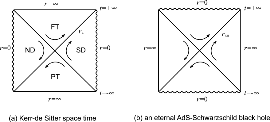
FIG. 1.: The upper/lower horizontal boundaries are future null infinity (${\cal I}^{+}$)/past null infinity (${\cal I}^{-}$) of $r=\infty$. For AdS-black hole, the horizontal lines belong to spacelike singularity of $r=0$. The vertical lines are spacelike singularity of $r=0$ for Kerr-de Sitter spacetime, while these are timelike infinity of $r=\infty$ for AdS-black hole. For Kerr-de Sitter spacetime, we call two regions with $0\leq r\leq 1$ as northern diamond (ND) and southern diamond (SD). An observer at $r=0$ is surrounded by a cosmological horizon $r=r_{+}$. Two regions with $1\leq r\leq\infty$ are called future triangle (FT) including ${\cal I}^{+}$ and past triangle (PT) including ${\cal I}^{-}$. The correct wave propagation is possible only in the southern diamond because a timelike Killing vector $\partial/\partial t$ is future-directed only in this region. The arrow($\rightarrow$) is the flow direction generated by the timelike Killing vector. Two of Kerr-de Sitter and AdS-black hole do not have a global timelike Killing vector.

There is no black hole horizon for three-dimensional Kerr-de Sitter space because the black hole degenerates to a conical singularity at the origin $r=0$. This space corresponds to the gravitational background of a point particle at $r=0$ in de Sitter space whose mass and spin are given by ${\cal M}$ and $J$, and the curvature radius of de Sitter space is given by $\ell$. Although this singularity gives rise to some difficulties to analyze the wave equation in the southern diamond (SD) of Kerr-de Sitter space, we introduce an observer within SD for our purpose. In this work we mainly consider the cosmological horizon with interest. For reference, we list the particle mass ${\cal M}$, Hawking temperature $T_{c}$, area of cosmological horizon ${\cal A}_{c}$, and angular velocity at the horizon $\Omega_{c}$ as

$${\cal M}=1-M,~{}~{}T_{c}=(r_{+}^{2}+r_{(-)}^{2})/2\pi\ell^{2}r_{+},~{}~{}{\cal A}_{c}=2\pi r_{+},~{}~{}\Omega_{c}=J/2r_{+}^{2}$$ (11)

which are measured by an observer at $r=\infty$. For $M=1,J=0$ case, one finds de Sitter solution which gives us with $r_{c}=\ell$ and $r_{-}=0$

$${\cal M}=0,~{}~{}T_{c}=1/2\pi\ell,~{}~{}{\cal A}_{c}=2\pi\ell,~{}~{}\Omega_{c}=0.$$ (12)

III Perturbation around Kerr-de Sitter solution

To study the propagation of all fields in Kerr-de Sitter space specifically, we introduce the small perturbation fields[16]

$$H_{t\phi r}=\bar{H}_{t\phi r}+{\cal H}_{t\phi r},~{}~{}~{}\Phi=0+\varphi,~{}~{}~{}g_{\mu\nu}=\bar{g}_{\mu\nu}+h_{\mu\nu}$$ (13)

around the background solution of Eq.(9). Here ${\cal H}_{t\phi r}=\partial_{[t}{\cal B}_{\phi r]}$. For convenience, we introduce the notation ${\hat{h}}_{\mu\nu}=h_{\mu\nu}-{\bar{g}}_{\mu\nu}h/2$ with $h=h^{\rho}_{~{}\rho}$. And then one needs to linearize Eqs.(2)-(4) to obtain

$$\delta R_{\mu\nu}(h)-\bar{\nabla}_{\mu}\bar{\nabla}_{\nu}\varphi-{1\over 2}\bar{H}_{\mu\rho\sigma}{\cal H}_{\nu}^{~{}\rho\sigma}+{1\over 2}\bar{H}_{\mu\rho\sigma}\bar{H}_{\nu\alpha}^{~{}~{}\sigma}h^{\rho\alpha} = 0,$$ (14)

$$\bar{\nabla}^{2}\varphi-{1\over 6}\Big{\{}2\bar{H}_{\mu\rho\sigma}{\cal H}^{\mu\rho\sigma}-3\bar{H}_{\mu\rho\sigma}\bar{H}^{\alpha\rho\sigma}h^{\mu}_{\alpha}\Big{\}} = 0,$$ (15)

$$\bar{\nabla}_{\mu}{\cal H}^{\mu\nu\rho}-(\bar{\nabla}_{\mu}h_{\beta}^{~{}\nu}){\bar{H}}^{\mu\beta\rho}+(\bar{\nabla}_{\mu}h_{\beta}^{~{}\rho}){\bar{H}}^{\mu\beta\nu}-(\bar{\nabla}_{\mu}{\hat{h}}_{~{}\alpha}^{\mu}){\bar{H}}^{\alpha\nu\rho}+(\partial_{\mu}\varphi)\bar{H}^{\mu\nu\rho} = 0,$$ (16)

where the Lichnerowicz operator $\delta R_{\mu\nu}(h)$ is given by

$$\delta R_{\mu\nu}=-{1\over 2}\bar{\nabla}^{2}h_{\mu\nu}+{\bar{R}}_{\sigma(\nu}h^{\sigma}_{~{}\mu)}-{\bar{R}}_{\sigma\mu\rho\nu}h^{\sigma\rho}+\bar{\nabla}_{(\nu}\bar{\nabla}_{|\rho|}{\hat{h}}^{\rho}_{~{}\mu)}.$$ (17)

These belong to the bare perturbation equations. It is desirable to examine whether we choose the physical perturbation by introducing a gauge which can simplify Eqs.(14)-(16) significantly. For this purpose we wish to count the physical degrees of freedom first. A symmetric traceless tensor has components of D(D+1)/2–1 in D-dimensions. D of them are eliminated by the gauge condition. Also D–1 are eliminated from our freedom to take further residual gauge transformations. Thus gravitational degrees of freedom are D(D+1)/2–1–D–(D–1)=D(D–3)/2. In three dimensions we have no propagating degrees of freedom for metric fluctuation $h_{\mu\nu}$. Also the Kalb-Romond two-form ${\cal B}_{\mu\nu}$ has no physical degrees of freedom for D=3. Hence the physical degree of freedom in the Kerr-de Sitter solution is just the dilaton $\varphi$.

Considering the $t$ and $\phi$-symmetries of the background spacetime Eq.(9), we can decompose $h_{\mu\nu}$ into frequency ($\omega$) and angular ($\mu=0,1,2,\cdots$) modes in these variables

$$h_{\mu\nu}(t,\phi,r)=e^{-i\omega t}e^{i\mu\phi}H_{\mu\nu}(r).$$ (18)

For simplicity, one chooses the same perturbation as in Eq.(18) for Kalb-Ramond field and dilaton as

$${\cal H}_{t\phi r}(t,\phi,r) =\bar{H}_{t\phi r}{\cal H}(t,\phi,r)=\bar{H}_{t\phi r}e^{-i\omega t}e^{i\mu\phi}\tilde{\cal H}(r),$$ (19)

$$\varphi(t,\phi,r) =e^{-i\omega t}e^{i\mu\phi}\tilde{\varphi}(r).$$ (20)

We stress again that this choice is possible only for D=3 because $h_{\mu\nu}$ and ${\cal H}_{\mu\nu\rho}$ are redundant fields. Since the dilaton is only a propagating mode, we focus on the dilaton equation (15). Eq.(14) is irrelevant to our analysis because it gives us a redundant relation. Eq.(15) can be rewritten as

$$\bar{\nabla}^{2}\varphi+{4\over l^{2}}(h-2{\cal H})=0.$$ (21)

We wish to decouple $h$ and ${\cal H}$ from the above $\varphi$-equation by making use of gauge-fixing and the Kalb-Ramond equation. If we start with full six degrees of freedom of Eq.(18), we should choose a gauge. Conventionally, we choose the harmonic gauge ($\bar{\nabla}_{\mu}{\hat{h}}^{\mu\rho}=0$) to describe the propagation of gravitons in D$>$3 dimensions[25]. A mixing between the dilaton and other fields of $h,{\cal H}$ can be disentangled with the harmonic gauge condition. Here we wish to introduce the dilaton gauge ($\bar{\nabla}_{\mu}\hat{h}^{\mu\rho}=h^{\mu\nu}\Gamma^{\rho}_{\mu\nu}$) for simplicity. Actually this gauge was designed for the study of the dilaton propagation[26]. We attempt to disentangle the last term in Eq.(21) by using both the dilaton gauge and Kalb-Ramond equation (16). Each component ($\rho=t,\phi,r$) of the dilaton gauge condition gives rise to

$$t : (\partial_{r}+{1\over r})h^{tr}-i\omega h^{tt}+i\mu h^{t\phi}+{1\over 2}i\omega h\bar{g}^{tt}-{1\over 2}i\mu h\bar{g}^{t\phi}=0,$$ (22)

$$\phi : (\partial_{r}+{1\over r})h^{\phi r}-i\omega h^{\phi t}+i\mu h^{\phi\phi}+{1\over 2}i\omega h\bar{g}^{\phi t}-{1\over 2}i\mu h\bar{g}^{\phi\phi}=0,$$ (23)

$$r : (\partial_{r}+{1\over r})h^{rr}-i\omega h^{rt}+i\mu h^{r\phi}-{1\over 2}(\partial_{r}h)\bar{g}^{rr}=0.$$ (24)

And each component ($\nu,\rho$) of the Kalb-Ramond equation (16) leads to

$$t\phi: -\partial_{r}(\varphi+{\cal H}-{h^{t}_{~{}t}}-{h^{\phi}_{~{}\phi}})+{1\over rf^{2}}\left(-M+{3r^{2}\over\ell^{2}}+{J^{2}\over 4r^{2}}\right)h^{r}_{~{}r}+i\omega h^{t}_{~{}r}-i\mu h^{\phi}_{~{}r}=0,$$ (25)

$$tr: -i\mu(\varphi+{\cal H}-h^{t}_{~{}t}-h^{r}_{~{}r})-{1\over r}h^{r}_{~{}\phi}+2f^{2}h^{\phi}_{~{}r}-\partial_{r}h^{r}_{~{}\phi}+i\omega h^{t}_{~{}\phi}=0,$$ (26)

$$\phi r: -i\omega(\varphi+{\cal H}-h^{\phi}_{~{}\phi}-h^{r}_{~{}r})+{1\over r}h^{r}_{~{}t}-{2rf^{2}\over\ell^{2}}h^{t}_{~{}r}+\partial_{r}h^{r}_{~{}t}+i\mu h^{\phi}_{~{}t}=0.$$ (27)

Solving six equations (22)-(27) simultaneously, one finds one constraint only

$$\partial_{\mu}(2\phi+2{\cal H}-h)=0,~{}~{}\mu=t,\phi,r$$ (28)

which leads to $h-2{\cal H}=2\varphi$. This means that $h$ and ${\cal H}$ becomes redundant if one follows the perturbations along Eqs.(18)-(20). It confirms that our counting for degrees of freedom is correct. We note here that the harmonic gauge with the Kalb-Ramond equation (16) leads to the same constraint as in Eq.(28). As a result, Eq.(21) becomes a decoupled dilaton equation

$$\bar{\nabla}^{2}\varphi+\frac{8}{\ell^{2}}\varphi=0$$ (29)

which can be rewritten explicitly as

$$\left[f^{2}\partial_{r}^{2}+\left\{{1\over r}(\partial_{r}rf^{2})\right\}\partial_{r}-{{J\mu\omega}\over{r^{2}f^{2}}}+{\omega^{2}\over f^{2}}+{(-M+{r^{2}/\ell^{2})}\over r^{2}f^{2}}j^{2}\right]\tilde{\varphi}+{8\over l^{2}}\tilde{\varphi}=0,$$ (30)

It is noted from Eq.(29) that if the last term is absent, it corresponds to the wave equation of a freely massive scalar in Kerr-de Sitter space. Comparing this dilaton equation with the freely massive scalar equation in Kerr-de Sitter space

$$\bar{\nabla}^{2}\varphi_{m}-m^{2}\varphi_{m}=0,$$ (31)

the dilaton propagates on Kerr-de Sitter space with the negative mass square of $m^{2}_{\varphi}=-8/\ell^{2}$. In Kerr-anti de Sitter space of the BTZ black hole, this is a good test field with $m^{2}_{\varphi}=8/\ell^{2}$. However the dilaton turns out to be a tachyon in the Kerr-de Sitter space background. Although in anti de Sitter space, the physical role of the tachyon is not clear, the dilatonic tachyon plays an important role in the study of the de Sitter physics[17]. Hence we have to do a further study for the tachyonic dilaton in the Kerr-de Sitter background.

IV solution to wave equation

It is not easy to solve the wave equation, Eq.(30), of the dilaton exactly on the southern diamond including the cosmological horizon ($r=r_{+}$) and the origin ($r=0$). The main difficulty comes from the fact that the black hole horizon degenerates to give a conical singularity at $r=0$. In other words, the Kerr-de Sitter solution represents a spinning point mass $1-M$ and spin $J$ within de Sitter space. Before solving Eq.(30), we present approximate solutions around $r=0$, $r^{2}=-r_{(-)}^{2}$ and $r=r_{+}$. For this purpose, see Fig. 2. Eq.(30) can be rewritten as

$${\tilde{\varphi}}^{\prime\prime}+{1\over f(r)}\left({f(r)\over r}+f^{\prime}(r)\right){\tilde{\varphi}}^{\prime}+{1\over f(r)}\left[-{{J\mu\omega}\over{r^{2}f(r)}}+{\omega^{2}\over f(r)}+{(-M+{r^{2}/\ell^{2})}\over r^{2}f(r)}\mu^{2}-m_{\varphi}^{2}\right]\tilde{\varphi}=0.$$ (32)

Each terms in Eq.(32) also can be written in terms of $r_{+}$ and $r_{(-)}$ as

$${1\over f(r)}\left({f(r)\over r}+f^{\prime}(r)\right)=-{1\over r}+{1\over{r_{+}+r}}-{1\over{r_{+}-r}}+{1\over{r+ir_{(-)}}}+{1\over{r-ir_{(-)}}},$$ (33)

$${1\over f(r)}\left[-{{J\mu\omega}\over{r^{2}f(r)}}+{\omega^{2}\over f(r)}+{(-M+{r^{2}/\ell^{2})}\over r^{2}f(r)}\mu^{2}-m_{\varphi}^{2}\right]$$ (34)

$$\hskip 10.0pt={r^{2}\ell^{4}\over{(r_{+}^{2}-r^{2})^{2}(r^{2}+r_{(-)}^{2})^{2}}}\left[\omega^{2}r^{2}-J\mu\omega+\left(-M+{r^{2}\over\ell^{2}}\right)\mu^{2}\right]-{r^{2}\ell^{2}m_{\varphi}^{2}\over{(r_{+}^{2}-r^{2})(r^{2}+r_{(-)}^{2})}}.$$ (35)

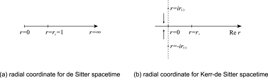
FIG. 2.: In de Sitter spacetime, $r=0$ is just a coordinate origin and $r=r_{c}=\ell$ is a position of the cosmological horizon. On the other hand, for $J\neq 0$ (Kerr-de Sitter space) $r=0$ becomes a conical singularity where a spinning source exists. Instead a role of $r=0$ in de Sitter space is split into $r=\pm ir_{(-)}$ ($r^{2}=-r_{(-)}^{2}$) in Kerr-de Sitter space. That is, if $J\rightarrow 0$, $\pm ir_{(-)}\rightarrow 0$. Further $r=r_{+}$ is a position of the cosmological horizon for $J\neq 0$. Hence, to solve the wave equation explicitly, one introduces a coordinate $z=r^{2}/\ell^{2}(0\leq z\leq 1)$ for de Sitter case, whereas one introduces $z={{r^{2}+r_{(-)}^{2}}\over{r_{+}^{2}+r_{(-)}^{2}}}$( $0\leq z\leq 1$) for Kerr-de Sitter case. For $J\neq 0$, $r=0$ corresponds to $z_{0}={{r_{(-)}^{2}}\over{r_{+}^{2}+r_{(-)}^{2}}}$ located between $z=0$ and $z=1$. Even though this complex picture (b) seems to be unphysical, it is useful for solving the wave equation in Kerr-de Sitter space.

A Approximate Solution around $r=0$

In this region the first term can be approximated as

$$\lim_{r\rightarrow 0}{1\over f(r)}\left({f(r)\over r}+f^{\prime}(r)\right)\simeq-{1\over r}+{8M\over J^{2}}r+{\cal O}(r^{3}).$$ (36)

and the second one takes approximately

$$\lim_{r\rightarrow 0}{1\over f(r)}\left[{\omega^{2}\over f(r)}-{{J\mu\omega}\over{r^{2}f(r)}}+{(-M+{r^{2}/\ell^{2})}\over r^{2}f(r)}\mu^{2}-m_{\varphi}^{2}\right]\simeq-C_{0}r^{2}+{\cal O}(r^{4}),$$ (37)

where

$$C_{0}={16\over J^{4}}\left[J\omega\mu+M\mu^{2}+{{m_{\varphi}^{2}J^{2}}\over 4}\right].$$ (38)

Hence Eq.(32) is reduced to

$${\tilde{\varphi}_{0}}^{\prime\prime}-{1\over r}{\tilde{\varphi}_{0}}^{\prime}-C_{0}r^{2}\tilde{\varphi}_{0}=0,$$ (39)

which has the solution

$${\tilde{\varphi}}_{0}\simeq A_{0}e^{-{{\sqrt{C_{0}}}\over 2}r^{2}}+B_{0}e^{{{\sqrt{C_{0}}}\over 2}r^{2}}.$$ (40)

This reflects that $r=0$ is a conical singularity, where a spinning source with $J\neq 0$ exists. In this sense Kerr-de Sitter space is different from de Sitter space. In the limit $J\rightarrow 0$, this solution is meaningless because of $\sqrt{C_{0}}\rightarrow\infty$.

B Approximate Solution around $r^{2}=-r_{(-)}^{2}$

In this region, $r$ is pure imaginary. It can be understood that $r$ is analytically extended here. We can split the limit $r^{2}\rightarrow-r_{(-)}^{2}$ into $r\rightarrow ir_{(-)}$ and $r\rightarrow-ir_{(-)}$. We consider the former because the latter gives us the same result. The first term takes

$$\lim_{r\rightarrow ir_{(-)}}{1\over f(r)}\left({f(r)\over r}+f^{\prime}(r)\right)\simeq{1\over{r-ir_{(-)}}}$$ (41)

and the second one is given by

$$\lim_{r\rightarrow ir_{(-)}}{1\over f(r)}\left[-{{J\mu\omega}\over{r^{2}f(r)}}+{\omega^{2}\over f(r)}+{(-M+{r^{2}/\ell^{2})}\over r^{2}f(r)}\mu^{2}-m_{\varphi}^{2}\right]$$ (42)

$$\hskip 10.0pt\simeq-{1\over 4}{1\over{(r-ir_{(-)})^{2}}}{\ell^{4}\over{(r_{+}^{2}+r_{(-)}^{2})^{2}}}\left[\omega^{2}r_{(-)}^{2}+J\mu\omega+\left(M+{r_{(-)}^{2}\over\ell^{2}}\right)\mu^{2}\right]$$ (43)

Hence Eq.(32) is approximated around $r=ir_{(-)}$ as

$${\tilde{\varphi}_{-+}}^{\prime\prime}+{1\over{r-ir_{(-)}}}{\tilde{\varphi}_{-+}}^{\prime}-{C_{-}\over{(r-ir_{(-)})^{2}}}{\tilde{\varphi}_{-+}}\simeq 0,$$ (44)

where

$$C_{-}={\ell^{4}\over{4(r_{+}^{2}+r_{(-)}^{2})^{2}}}\left[J\mu\omega+\omega^{2}r_{(-)}^{2}+\left(M+{r_{(-)}^{2}\over\ell^{2}}\right)\mu^{2}\right].$$ (45)

Here we have $C_{-}>0$ and in the de Sitter limit, $C_{-}\to\mu^{2}/4$. Eq.(44) has the solution

$${\tilde{\varphi}}_{-+} = A_{-+}(r-ir_{(-)})^{\sqrt{C_{-}}}+B_{-+}(r-ir_{(-)})^{-\sqrt{C_{-}}}$$ (46)

$$= A_{-+}e^{\sqrt{C_{-}}\ln(r-ir_{(-)})}+B_{-+}e^{-\sqrt{C_{-}}\ln(r-ir_{(-)})}.$$ (47)

Now we consider the latter. In this case two terms are given approximately by

$$\lim_{r\rightarrow-ir_{(-)}}{1\over f(r)}\left({f(r)\over r}+f^{\prime}(r)\right)\simeq{1\over{r+ir_{(-)}}}$$ (48)

and

$$\lim_{r\rightarrow-ir_{(-)}}{1\over f(r)}\left[-{{J\mu\omega}\over{r^{2}f(r)}}+{\omega^{2}\over f(r)}+{(-M+{r^{2}/\ell^{2})}\over r^{2}f(r)}\mu^{2}-m_{\varphi}^{2}\right]\simeq-{C_{-}\over{(r+ir_{(-)})^{2}}}$$ (49)

Then Eq.(32) is approximated around $r=-ir_{(-)}$ as

$${\tilde{\varphi}_{--}}^{\prime\prime}+{1\over{r+ir_{(-)}}}{\tilde{\varphi}_{--}}^{\prime}-{C_{-}\over{(r+ir_{(-)})^{2}}}{\tilde{\varphi}_{--}}\simeq 0.$$ (50)

The solution to Eq.(50) is the same form as in Eq.(47),

$${\tilde{\varphi}}_{--} = A_{--}(r+ir_{(-)})^{\sqrt{C_{-}}}+B_{--}(r+ir_{(-)})^{-\sqrt{C_{-}}}$$ (51)

$$= A_{--}e^{\sqrt{C_{-}}\ln(r+ir_{(-)})}+B_{--}e^{-\sqrt{C_{-}}\ln(r+ir_{(-)})}.$$ (52)

Taking the limit of $r_{(-)}\rightarrow 0$ ($J\rightarrow 0$), Eqs.(47) and (52) give the same solution for consistency, which implies that

$$A_{-+}=A_{--}\equiv A_{-},$$ (53)

$$B_{-+}=B_{--}\equiv B_{-}.$$ (54)

Using these, we express Eqs.(47) and (52) as

$${\tilde{\varphi}}_{-+} = A_{-}(r-ir_{(-)})^{\sqrt{C_{-}}}+B_{-}(r-ir_{(-)})^{-\sqrt{C_{-}}}$$ (55)

$$= A_{-}e^{\sqrt{C_{-}}\ln(r-ir_{(-)})}+B_{-}e^{-\sqrt{C_{-}}\ln(r-ir_{(-)})},$$ (56)

$${\tilde{\varphi}}_{--} = A_{-}(r+ir_{(-)})^{\sqrt{C_{-}}}+B_{-}(r+ir_{(-)})^{-\sqrt{C_{-}}}$$ (57)

$$= A_{-}e^{\sqrt{C_{-}}\ln(r+ir_{(-)})}+B_{-}e^{-\sqrt{C_{-}}\ln(r+ir_{(-)})}.$$ (58)

Note that if one takes the limit of $r_{(-)}\rightarrow 0$, Eqs.(44) and (50) becomes

$${\tilde{\varphi}_{-0}}^{\prime\prime}+{1\over r}{\tilde{\varphi}_{-0}}^{\prime}-{\mu^{2}\over{4M}}{1\over r^{2}}{\tilde{\varphi}_{-0}}=0,$$ (59)

which has the Kerr-de Sitter solution at $r=0$ when $J=0$.

$${\tilde{\varphi}}_{-0} = A_{-}r^{\mu\over{2\sqrt{M}}}+B_{-}r^{-{\mu\over{2\sqrt{M}}}}$$ (60)

$$= A_{-}e^{{\mu\over{2\sqrt{M}}}\ln r}+B_{-}e^{-{\mu\over{2\sqrt{M}}}\ln r}.$$ (61)

This approximate solution is obtained by taking the limit $r_{(-)}\rightarrow 0$, followed after $r\rightarrow 0$. On the other hand, if we take the limit $r\rightarrow 0$, followed after $r_{(-)}\rightarrow 0$, then Eq.(32) becomes

$$\tilde{\varphi}_{0-}^{\prime\prime}+{1\over r}\tilde{\varphi}_{0-}^{\prime}-{\mu^{2}\over M}{1\over r^{2}}\tilde{\varphi}_{0-}=0.$$ (62)

This equation is actually different from Eq.(59) and has the de Sitter solution at $r=0$

$$\tilde{\varphi}_{0-} = A_{-}^{\prime}r^{{\mu}\over{\sqrt{M}}}+B_{-}^{\prime}r^{-{\mu}\over{\sqrt{M}}}$$ (63)

$$= A_{-}^{\prime}e^{{{\mu}\over{\sqrt{M}}}\ln r}+B_{-}^{\prime}e^{{-{\mu}\over{\sqrt{M}}}\ln r}.$$ (64)

Hence the order of taking a limit is important to derive the correct solution.

C Approximate Solution around $r=r_{+}$

In this region two terms can obtained by using (33) and (35) as

$$\lim_{r\rightarrow r_{+}}{1\over f(r)}\left({f(r)\over r}+f^{\prime}(r)\right)\simeq-{1\over{r_{+}-r}}$$ (65)

and

$$\lim_{r\rightarrow r_{+}}{1\over f(r)}\left[-{{J\mu\omega}\over{r^{2}f(r)}}+{\omega^{2}\over f(r)}+{(-M+{r^{2}/\ell^{2})}\over r^{2}f(r)}\mu^{2}-m_{\varphi}^{2}\right]$$ (66)

$$\hskip 10.0pt\simeq{1\over 4}{1\over{(r_{+}-r)^{2}}}{\ell^{4}\over{(r_{+}^{2}+r_{(-)}^{2})^{2}}}\left[\omega^{2}r_{+}^{2}-J\mu\omega+\left(-M+{r_{+}^{2}\over\ell^{2}}\right)\mu^{2}\right]$$ (67)

Hence Eq.(32) is approximated around $r=r_{+}$ as

$${\tilde{\varphi}_{+}}^{\prime\prime}-{1\over{r_{+}-r}}{\tilde{\varphi}_{+}}^{\prime}+{C_{+}\over{(r_{+}-r)^{2}}}{\tilde{\varphi}_{+}}\simeq 0,$$ (68)

where

$$C_{+}={\ell^{4}\over{4(r_{+}^{2}+r_{(-)}^{2})^{2}}}\left[\omega^{2}r_{+}^{2}-J\mu\omega+\left(-M+{r_{+}^{2}\over\ell^{2}}\right)\mu^{2}\right].$$ (69)

We assume that $C_{+}>0$ for our purpose. This is valid because in the de Sitter limit of $J\rightarrow 0$, $r_{+}\rightarrow\ell$, $M\rightarrow 1$, one finds that $C_{+}\rightarrow\omega^{2}\ell^{2}/4>0$. Then Eq.(68) has the travelling wave solution

$${\tilde{\varphi}}_{+} = A_{+}(r_{+}-r)^{i\sqrt{C_{+}}}+B_{+}(r_{+}-r)^{-i\sqrt{C_{+}}}$$ (70)

$$= A_{+}e^{i\sqrt{C_{+}}\ln(r_{+}-r)}+B_{+}e^{-i\sqrt{C_{+}}\ln(r_{+}-r)}.$$ (71)

D Exact Solution for the whole region

Now we can convert Eq.(30) to a hypergeometric equation by introducing variable $z\equiv(r^{2}+r_{(-)}^{2})/(r_{+}^{2}+r_{(-)}^{2})$ as (see Fig. 2)

$${{d^{2}\tilde{\varphi}}\over{dz^{2}}}+\left({1\over z}-{1\over{1-z}}\right){{d\tilde{\varphi}}\over{dz}}-\left({C_{-}\over z}-{C_{+}\over{1-z}}+{{m_{\varphi}^{2}\ell^{2}}\over 4}\right){{\tilde{\varphi}}\over{z(1-z)}}=0,$$ (72)

where $m_{\varphi}^{2}\ell^{2}=-8$, $C_{+}$ and $C_{-}$ are defined in Eqs.(69) and (45). Note that $z\to 0$ corresponds to $r\to\pm ir_{(-)}$. With a new function $\tilde{\varphi}=z^{\alpha}(1-z)^{\beta}\bar{\varphi}$, Eq.(72) can be transformed into

$$z(1-z)\bar{\varphi}^{\prime\prime} + \left[1+2\alpha-(2+2\alpha+2\beta)\right]\bar{\varphi}^{\prime}$$ (73)

$$- \left[(\alpha+\beta)(\alpha+\beta+1)+{{m^{2}\ell^{2}}\over 4}-{{\alpha^{2}-C_{-}}\over z}-{{\beta^{2}+C_{+}}\over{1-z}}\right]\bar{\varphi}=0.$$ (74)

This equation leads to the standard hypergeometric equation if we choose $\alpha=\sqrt{C_{-}}$ and $\beta=i\sqrt{C_{+}}$. Other choices of $\alpha$ and $\beta$ are irrelevant to our purpose[12]. Then a normalizable solution near $z=0$ is

$$\tilde{\varphi}=E_{0}z^{\sqrt{C_{-}}}(1-z)^{i\sqrt{C_{+}}}F(a,b,c;z),$$ (75)

with

$$a = {1\over 2}\left(1+2\sqrt{C_{-}}+2i\sqrt{C_{+}}+\sqrt{1-m^{2}\ell^{2}}\right)$$ (76)

$$b = {1\over 2}\left(1+2\sqrt{C_{-}}+2i\sqrt{C_{+}}-\sqrt{1-m^{2}\ell^{2}}\right)$$ (77)

$$c = 1+2\sqrt{C_{-}}$$ (78)

and an arbitrary constant $E_{0}$. If we take the de Sitter limit ($J\to 0$, $M\rightarrow 1$, $r_{+}\rightarrow\ell$), the above quantities are reduced to[12]

$$\sqrt{C_{-}}\to{\mu\over{2}},~{}~{}\sqrt{C_{+}}\to{{\omega\ell}\over{2}}$$ (79)

$$a\to{1\over 2}(1+\mu+i\omega\ell+\sqrt{1-m_{\varphi}^{2}\ell^{2}}),$$ (80)

$$b\to{1\over 2}(1+\mu+i\omega\ell-\sqrt{1-m_{\varphi}^{2}\ell^{2}}),$$ (81)

$$c\to 1+\mu.$$ (82)

We transform Eq.(75) to a region around $z=1$ using the relation between the hypergeometric functions

$$F(a,b,c;z)=\frac{\Gamma(c)\Gamma(c-a-b)}{\Gamma(c-a)\Gamma(c-b)}F(a,b,a+b-c+1;1-z)$$ (83)

$$~{}~{}+\frac{\Gamma(c)\Gamma(a+b-c)}{\Gamma(a)\Gamma(b)}(1-z)^{c-a-b}F(c-a,c-b,-a-b+c+1;1-z).$$ (84)

Using $1-z\simeq 2r_{+}(r_{+}-r)/(r_{+}^{2}+r_{(-)}^{2})$$=2r_{+}/(r_{+}^{2}+r_{(-)}^{2})e^{\ln(r_{+}-r)}$, one finds from Eqs.(75) and (71) the following form :

$$\tilde{\varphi}_{z\rightarrow 1}\equiv\tilde{\varphi}_{in}+\tilde{\varphi}_{out}=A_{+}e^{i\sqrt{C_{+}}\ln(r_{+}-r)}+B_{+}e^{-i\sqrt{C_{+}}\ln(r_{+}-r)},$$ (85)

where $A_{+}$ and $B_{+}$ are determined as

$$A_{+} = E_{0}\left({{2r_{+}}\over{r_{+}^{2}+r_{(-)}^{2}}}\right)^{i\sqrt{C_{+}}}{{\Gamma(c)\Gamma(c-a-b)}\over{\Gamma(c-a)\Gamma(c-b)}}$$ (86)

$$B_{+} = E_{0}\left({{2r_{+}}\over{r_{+}^{2}+r_{(-)}^{2}}}\right)^{-i\sqrt{C_{+}}}{{\Gamma(c)\Gamma(a+b-c)}\over{\Gamma(a)\Gamma(b)}}$$ (87)

Note that $A_{+}=B_{+}^{*}$ if $E_{0}$ is chosen to be real. Because we find $|A_{+}/B_{+}|=1$, two travelling waves $(\tilde{\varphi}_{in}e^{-i\omega t},~{}\tilde{\varphi}_{out}e^{-i\omega t})$ have amplitudes of the same magnitude. The absolute square of the amplitude of the tachyonic dilaton must be proportional to the flux. As a result we conclude that an outgoing $(\leftarrow)$ wave is reflected back to give an ingoing $(\rightarrow)$ wave by the potential. This interpretation is in accordance with the classical picture of what the particle goes on[27]. Actually there is no wave propagating truly toward a conical singulaity.

V No absorption cross section

The absorption coefficient by the cosmological horizon is defined by the ratio of the outgoing flux at $r=0$ to the outgoing flux at $r=r_{+}$ as

$${\cal A}=\frac{{\cal F}_{out}(r=r_{+})}{{\cal F}_{out}(r=0)}.$$ (88)

Since the wave function near $r=0$ is real (see Eq.(40)), its flux should be zero (${\cal F}_{out}(r=0)=0$). Also ${\cal F}_{out}(r=r_{+})$ can be calculated as

$${\cal F}_{out}(r=r_{+})={{2\pi}\over i}\left.\left[\tilde{\varphi}_{out}^{*}(r_{+}-r)\partial_{r}\tilde{\varphi}_{out}-\tilde{\varphi}_{out}(r_{+}-r)\partial_{r}\tilde{\varphi}_{out}^{*}\right]\right|_{r=r_{+}}=4\pi\sqrt{C_{+}}\left|B_{+}\right|^{2}.$$ (89)

On the other hand, the ingoing flux at $r=r_{+}$ takes the form

$${\cal F}_{in}(r=r_{+})={{2\pi}\over i}\left.\left[\tilde{\varphi}_{in}^{*}(r_{+}-r)\partial_{r}\tilde{\varphi}_{in}-\tilde{\varphi}_{in}(r_{+}-r)\partial_{r}\tilde{\varphi}_{in}^{*}\right]\right|_{r=r_{+}}=4\pi\sqrt{C_{+}}\left|A_{+}\right|^{2}.$$ (90)

Here we find ${\cal F}_{out}(r=r_{+})={\cal F}_{in}(r=r_{+})$ because of $|B_{+}|=|A_{+}|$. This means that there is no absorption of the tachyonic dialton in Kerr-de Sitter space. This is obvious because there is no wave propagating truly toward a conical singulaity. This can be also checked by the zero flux of ${\cal F}_{out}(r=0)=0$. As a result, the absorption cross section $\sigma_{\rm abs}$ defined ${\cal A}/\omega$ in three dimensions is zero,

$$\sigma_{\rm abs}=0$$ (91)

even if one gets ${\cal F}_{out}(r=0)=0$. One finds the same situation if one uses $r=\pm ir_{(-)}$ instead of $r=0$ to calculate the denominator of Eq.(88).

VI discussion

We study the wave equation of the tachyonic dilaton which propagates on the southern diamond of three-dimensional Kerr-de Sitter space. We wish to point out that this space is somewhat different from de Sitter space because it contains a conical singularity at $r=0$. First we find approximate solutions at $r=\pm ir_{(-)},~{}0,~{}r_{+}$ to the wave equation. We compute the absorption cross section to investigate its cosmological horizon by transforming the wave equation into the standard hypergeometric equation. By analogy of the quantum mechanics of the wave scattering under the potential step, it turns out that there is no absorption of the tachyonic dilaton in Kerr-de Sitter space in the semiclassical approach. This means that Kerr-de Sitter space is usually stable and in thermal equilibrium, unlike the black hole. The cosmological horizon not only emits radiation but also absorbs that previously emitted by itself at the same rate, keeping the curvature radius $\ell$ of Kerr-de Sitter space fixed. This can be proved by the relation of ${\cal F}_{out}(r=r_{+})={\cal F}_{in}(r=r_{+})$ and ${\cal F}_{out/in}(r=0)=0$. This exactly coincides with the wave propagation of the energy $E$ under the potential step with $0<E<V_{0}$ which shows the classical picture of what the particle goes on[27]. Here we find a nature of the eternal Kerr-de Sitter horizon[28], which means that its cosmological constant $\Lambda=1/l^{2}$ remains unchanged, as like the eternal AdS-black hole[29].

Finally we remark on a few of results. 1) A conical singularity at $r=0$ is not so important to derive our conclusion of no absorption in Kerr-de Sitter space. In Kerr-de Sitter space, a role of the coordinate origin $r=0$ in de Sitter space is replaced by not $r=0$ but $r=\pm r_{(-)}$. 2) In the black hole study we usually avoid a naked singularity by making use of the cosmic censorship hypothesis. That is, the working region is from the event horizon to the infinity. However, in the de Sitter physics, we cannot avoid a singularity because our interesting region is the southern diamond (SD) in Fig.1 which includes a conical singulaity. 3) In this work we deal directly with a conical singularity to find the absorption cross section of the dilatonic tachyon. 4) Either the presence of a conical singularity (Kerr-de Sitter space) or the absence of a conical singularity (de Sitter space) gives us the same zero absorption cross section. This implies that a conical singularity does not affect on the absorption cross section of any scalar wave with the mass square $m^{2}$ including the dilatonic tachyon with $m^{2}_{\varphi}=-8/\ell^{2}$. In this sense the mass of a scalar wave does not play an important role in propagation of Kerr-de Sitter space.

REFERENCES

• [1] S. Perlmutter et al.(Supernova Cosmology Project), Astrophys. J. 483, 565(1997)[astro-ph/9608192].
• [2] R. R. Caldwell, R. Dave, and P. J. Steinhard, Phys. Rev. Lett. 80, 1582(1998)[astro-ph/9708069].
• [3] P. M. Garnavich et al., Astrophys. J. 509, 74(1998)[astro-ph/9806396].
• [4] E.Witten, “Quantum Gravity in de Sitter Space", hep-th/0106109.
• [5] S. Hellerman, N. Kaloper, and L. Susskind, JHEP 0106, 003(2001)[hep-th/0104180].
• [6] W. Fischler, A. Kashani-Poor, R. McNees, and S. Paban, JHEP 0107, 003 (2001)[hep-th/0104181].
• [7] R.Bousso, JHEP 0011, 038 (2000)[hep-th/0010252]; R. Bousso, JHEP 0104, 035 (2001)[hep-th/0012052]; S. Nojiri and D. Odintsov, Phys.Lett. B519, 145 (2001)[ hep-th/0106191]; D. Klemm, “Some Aspects of the de Sitter/CFT correspondence", hep-th/0106247 ; M. Spradlin, A. Strominger, and A. Volovich, “Les Houches Lectures on De Sitter Space", hep-th/0110007; S. Cacciatori and D. Klemm, “The Asymptotic Dynamics of de Sitter Gravity in three Dimensions", hep-th/0110031; A. C. Petkou and G. Siopsis, “dS/CFT correspondence on a brane", hep-th/0111085. V. Balasubramanian, J. de Boer, and D. Minic, “Mass, Entropy and Holography in Asymptotically de Sitter Spaces", hep-th/0110108; R. G. Cai, Y. S. Myung, and Y. Z. Zhang, “Check of the Mass Bound Conjecture in de Sitter Space", hep-th/0110234; Y. S. Myung, Mod. Phys. Lett.A16, 2353(2001)[hep-th/0110123]; R. G. Cai, “Cardy-Verlinde Formula and Asymptotically de Sitter Spaces", hep-th/0111093; A. M. Ghezelbach and R. B. Mann, JHEP 0201, 005 (2002)[hep-th/0111217]; M. Cvetic, S. Nojiri, and S.D. Odintsov, “Black Hole Thermodynamics and Negative Entropy in deSitter and Anti-deSitter Einstein-Gauss-Bonnet gravity", hep-th/0112045; Y. S. Myung, “Dynamic dS/CFT correspondence using the brane cosmology", hep-th/0112140; R. G. Cai, “Cardy-Verlinde Formula and Thermodynamics of Black Holes in de Sitter Spaces", hep-th/0112253; S. R. Das, “Thermality in de Sitter and Holography", hep-th/0202008; F. Lebond, D. Marolf and R. C. Myers, “Tall tales from de Sitter space I: Renorlamization group flows", hep-th/0202094; A. J. Medved, “How Not to Construct an Asymptotically de Sitter Universe", hep-th/0203191; G. Siopsis, “An ADS/DS Duality for a Scalar Particle", hep-th/0203208; T. R. Govindarajan, R. K. Kaul, and V. Suneeta, “Quantum Gravity on $dS_{3}$, hep-th/0203219; C. Teitelboim, “Gravitational Thermodynamics of Schwarzschild de Sitter space", hep-th/ 0203258; D. Klemm and L. Vanzo, “De Sitter gravity and Liouville Theory", hep-th/0203368.
• [8] A. Strominger, JHEP 0110, 034 (2001)[hep-th/0106113]; A. J. Tolley and N. Turok, “Quantization of the massless minimally coupled scalar field and the dS/CFT correspondence", hep-th/0108119.
• [9] R. Bousso, A. Maloney, and A. Strominger, “Conformal vacua and entropy in de Sitter space", hep-th/0112218.
• [10] M. Spradlin and A. Volovich, “Vacuum states and the S-matrix in dS/CFT", hep-th/0112223.
• [11] Y. S. Myung, “Absorption cross section in de Sitter space", hep-th/0201176.
• [12] Y. S. Myung and H. W. Lee, “No absorption in de Sitter space", hep-th/0302148.
• [13] Z. Chang and C.-B. Guan, “Dynamics of Massive Scalar Fields in dS Space and the dS/CFT Correspondence", hep-th/0204014; E. Abdalla, B. Wang, A. Lima-Santos and W. G. Qiu, “Support of dS/CFT correspondence from perturbations of three dimensional spacetime", hep-th/0204030.
• [14] G. Horowitz and D. Welch, Phys. Rev. Lett. 71, 328(1993); N. Kaloper, Phys. Rev. D48, 2598(1993); A. Ali and A. Kumar, Mod. Phys. Lett. A8, 2045(1993).
• [15] M. Banados, C. Teitelboim and A. Zanelli, Phys. Rev. Lett. 69, 1849(1992).
• [16] D. B. Birmingham, I. Sachs and S. Sen, Phys. Lett. B413, 281(1997); H.W. Lee, N. J. Kim, and Y. S. Myung, Phys. Rev. D58, 084022 (1988)[hep-th/9803080]; H.W. Lee, N. J. Kim, and Y. S. Myung, Phys. Lett. B441, 83(1988)[hep-th/9803227]; H.W. Lee and Y. S. Myung, Phys. Rev. D58, 104013 (1988)[hep-th/9804095].
• [17] H.W. Lee and Y. S. Myung, Phys. Lett. B537, 117(2002) [hep-th/0204083].
• [18] C. Callan, S. Gubser, I. Klebanov, and A. Tseytlin, Nucl. Phys. B489, 65(1997)[hep-th/9610172]; M. Karsnitz and I. Klebanov, Phys. Rev. D56, 2173(1997)[hep-th/9703216]; B. Kol and A. Rajaraman, Phys. Rev. D56, 983(1997)[hep-th/9608126]; M. Cvetic and F. Larsen, Nucl. Phys. B506, 107(1997)[hep-th/9706071].
• [19] A. Dhar, G. Mandal, and S. Wadia ,Phys. Lett. B388, 51(1996) [hep-th/9605234]; S. Das, G. Gibbons and S. Mathur, Phys. Rev. Lett. 78, 417(1977)[hep-th/9609052].
• [20] M. I. Park, Phys.Lett. B440, 275(1998) [hep-th/9806119]; M. Banados, T. Brotz and M. Ortiz, Phys. Rev. D59, 046002(1999)[hep-th/9807216].
• [21] W. T. Kim, Phys. Rev. D59, 047503(1999)[hep-th/9810169]; F. Lin and Y. Wu, Phys. Lett. B453, 222 (1999)[hep-th/9901147].
• [22] S. Shankaranarayanan, “Temperature and entropy of Schwarzschild-de Sitter space-time", gr-qc/0301090.
• [23] W. T. Kim, J.J. Oh, and K. H.Yee, “Scattering amplitudes and thermal temperatures of the Schwarzschild-de Sitter black holes", hep-th/ 0201117.
• [24] H. Suzuki, E. Takasugi, and H. Umetsu, Prog. Theor. Phys. 103, 103 (2000)[gr-qc/9911079].
• [25] S. Weinberg, Gravitation and Cosmology (Wiley, New York,1972), p.254.
• [26] H.W. Lee, N. J. Kim, Y. S. Myung, and J. Y. Kim, Phys. Rev. D57, 7361(1998)[hep-th/9801152].
• [27] E. H. Wichmann, quantum physics-berkely physics course 4 (Macgraw-hill, 1971, New York), p.280.
• [28] L. Dyson, M. Kleban, and L. Susskind, “Disturbing Implications of a Cosmological constant", hep-th/0208013.
• [29] J. Maldacena. “Eternal black hole in Anti de Sitter", hep-th/0106112.