Stability of Neutral Fermi Balls with Multi-Flavor Fermions

Abstract

A Fermi ball is a kind of non-topological soliton, which is thought to arise from the spontaneous breaking of an approximate $Z_{2}$ symmetry and to contribute to cold dark matter. We consider a simple model in which fermion fields with multi-flavors are coupled to a scalar field through Yukawa coupling, and examine how the number of the fermion flavors affects the stability of the Fermi ball against the fragmentation. (1)We find that the Fermi ball is stable against the fragmentation in most cases even in the lowest order thin-wall approximation. (2)We then find that in the other specific cases, the stability is marginal in the lowest order thin-wall approximation, and the next-to-leading order correction determines the stable region of the coupling constants; We examine the simplest case where the total fermion number $N_{i}$ and the Yukawa coupling constant $G_{i}$ of each flavor $i$ are common to the flavor, and find that the Fermi ball is stable in the limited region of the parameters and has the broader region for the larger number of the flavors.

I INTRODUCTION

A Fermi ball MAC ; MOR , a kind of non-topological soliton LEE , is composed of three parts: a false vacuum domain, a domain wall enveloping the domain, and zero-mode fermions DVA confined in the domain wall. The Fermi ball is stabilized owing to the dynamical balance of the shrinking force due to the surface energy and the volume energy, and the expanding force due to the Fermi energy. The Fermi ball is thought to be a candidate for one kind of cold dark matter in the present universe ARA .

Macpherson and Campbell pointed out that such stability holds good only for the spherical shape of the Fermi ball MAC . They further showed that the Fermi ball is not stable against the deformation of the spherical shape, and thus flattens and fragments into tiny Fermi balls. The destabilization is caused by the volume energy of the Fermi ball.

We, however, pointed out that the perturbative correction due to the domain wall curvature can stabilize the Fermi ball when the volume energy is small enough compared to the curvature effect YOS ; OGU . In case of a simple model with a single fermion flavor, we found that only in the quite narrow region of the parameters does the Fermi ball become stable.

The purpose of the present paper is to examine how the fermion content of the model affects the stability of the Fermi ball. As an example, we consider an extended model in which fermions with multi-flavors are coupled to a scalar field through Yukawa coupling. Since the Pauli’s exclusion principle does not apply to the different flavors of the fermions, the stable region of the parameters is expected to broaden.

II STABILITY OF FERMI BALL

We consider the following Lagrangian density,

$${\cal L}=\frac{1}{2}(\partial_{\mu}\phi)^{2}+\sum_{i=1}^{n}\overline{\Psi_{i}}(i\gamma_{i}^{\mu}\partial_{\mu}-G_{i}\phi)\Psi_{i}-U(\phi)~{}~{},$$ (1)

where the scalar potential $U(\phi)$ is given by

$$U(\phi)=\frac{\lambda}{8}(\phi^{2}-v^{2})^{2}+\Delta(\phi)~{}~{}.$$ (2)

If the quantity $|\Delta(v)-\Delta(-v)|$ is zero, the Lagrangian density is invariant under the $Z_{2}$ transformation, $\phi\leftrightarrow-\phi$. There is, however, a small but a finite quantity $|\Delta(v)-\Delta(-v)|\simeq\Lambda\ll\lambda v^{4}$, where the invariance is not a strict one.

We consider a spherical Fermi ball with the radius $R$, and assume that the wave function $\Psi_{i}$ and the boson $\phi$ are static and that $\phi$ depends only on the radial coordinate $r$. Let $\Psi_{i}$ be the eigenfunction of the total angular momentum squared ${\vec{\bf J}}^{2}$, the $z$ component ${\bf J_{z}}$ and the parity ${\bf P}$ with the eigenvalues of $J(J+1)$, $M$ and $(-1)^{J-\omega/2}$ ($\omega=\pm 1$), respectively. Then, $\Psi_{i}$ is written as

$$\Psi_{i}(\vec{x})=\frac{1}{r}\left(\begin{array}[]{l}f(r){\cal Y}_{lJ}^{M}(\theta,\varphi)\\ g(r){\cal Y}_{l^{\prime}J}^{M}(\theta,\varphi)\end{array}\right)~{}~{},$$ (5)

where ${\cal Y}_{lJ}^{M}$ and ${\cal Y}_{l^{\prime}J}^{M}=({\vec{\sigma}}{\vec{x}}/r){\cal Y}_{lJ}^{M}$ are the spherical spinors having the eigenvalues $J$ and $M$, with $J=l+\omega/2=l^{\prime}-\omega/2$. Substituting Eq.(5) into the Lagrangian $L=\int{\rm d}^{3}x~{}{\cal L}$, we obtain

$$L[\phi,\psi_{i}]=-\int_{0}^{\infty}{\rm d}r~{}\left[4\pi r^{2}\left\{\frac{1}{2}\left(\frac{{\rm d}\phi}{{\rm d}r}\right)^{2}+U(\phi)\right\}+\sum_{i}\sum_{KM}\psi_{i}^{\dagger}H_{f}\psi_{i}\right]~{}~{},$$ (6)

where

$$H_{f}=\sigma_{1}\frac{1}{i}\frac{{\rm d}}{{\rm d}r}+\sigma_{2}\frac{K}{r}+\sigma_{3}G_{i}\phi~{}~{},$$ (7)

with $K=\omega(J+\frac{1}{2})$ and $\psi_{i}(r)={f(r)\choose g(r)}$. Since the Fermi ball is a ground state with a fixed number of fermions,

$$N_{i}=\int{\rm d}^{3}x~{}\Psi_{i}^{\dagger}\Psi_{i}~{}~{},$$ (8)

we obtain the wave function $\psi_{i}$ and the scalar field $\phi$ by extremizing

$$L_{\epsilon}[\phi,\psi_{i}]=L[\phi,\psi_{i}]+\sum_{i}\epsilon_{i}\left(\sum_{KM}\int_{0}^{\infty}{\rm d}r~{}\psi_{i}^{\dagger}\psi_{i}-N_{i}\right)~{}~{},$$ (9)

with the Lagrange multipliers $\epsilon_{i}$. The energy of the Fermi ball is expressed in terms of the fields as

$$E=\int_{0}^{\infty}{\rm d}r~{}\left[4\pi r^{2}\left\{\frac{1}{2}\left(\frac{{\rm d}\phi}{{\rm d}r}\right)^{2}+U(\phi)\right\}\right]+\sum_{i}\sum_{KM}\epsilon_{i}$$ (10)

where $\epsilon_{i}$ is equal to the Fermi energy $\epsilon_{i}=\int_{0}^{\infty}{\rm d}r~{}\psi_{i}^{\dagger}H_{f}\psi_{i}$ and $\psi_{i}$ is normalized as $\int_{0}^{\infty}{\rm d}r~{}\psi_{i}^{\dagger}\psi_{i}=1$. In order to estimate the energy of the Fermi ball, we take the thin-wall approximation and obtain the correction due to the finite curvature radius $R$ by the perturbation with respect to $1/R$. We expand $\phi$, $\psi_{i}$, and $H_{f}$ in the power of $1/R$,

$$\left\{\begin{array}[]{l}\phi=\phi_{0}+\phi_{1}+\cdots\\ \psi_{i}=\psi_{i0}+\psi_{i1}+\cdots\\ H_{f}=H_{0}+H_{1}+H_{2}+\cdots~{}~{},\end{array}\right.$$ (14)

where

$$H_{0} = \sigma_{1}\frac{1}{i}\frac{{\rm d}}{{\rm d}r}+\sigma_{2}\frac{K}{R}+\sigma_{3}G_{i}\phi_{0}$$

$$H_{1} = -\sigma_{2}\frac{Kw}{R^{2}}+\sigma_{3}G_{i}\phi_{1}$$

$$H_{2} = \sigma_{2}\frac{Kw^{2}}{R^{3}}~{}~{},$$ (15)

with $w=r-R$. From $\delta L_{\epsilon}/\delta\phi=\delta L_{\epsilon}/\delta\psi_{i}^{\dagger}=0$, we obtain the equations of motion,

$$H_{0}\psi_{i0}=\epsilon_{i0}\psi_{i0}$$ (16)

$$\frac{{\rm d}^{2}\phi_{0}}{{\rm d}w^{2}}=\left.\frac{\partial U}{\partial\phi}\right|_{\phi=\phi_{0}}+\sum_{i}\frac{G_{i}}{4\pi R^{2}}\sum_{KM}\psi_{i0}^{\dagger}\sigma_{3}\psi_{i0}~{}~{},$$ (17)

and

$$(H_{0}-\epsilon_{i0})\psi_{i1}=-(H_{1}-\epsilon_{i1})\psi_{i0}$$ (18)

$$\left[\frac{{\rm d}^{2}}{{\rm d}w^{2}}-\left.\frac{\partial^{2}U}{\partial\phi^{2}}\right|_{\phi=\phi_{0}}\right]\phi_{1}=-\frac{2}{R}\frac{{\rm d}\phi_{0}}{{\rm d}w}+\sum_{i}\frac{G_{i}}{2\pi R^{2}}\sum_{KM}\psi_{i0}\sigma_{3}\psi_{i1}~{}~{}.$$ (19)

Neglecting $\Delta(\phi)$ in the scalar potential $U(\phi)$ for simplicity, we have analytic solutions for $\phi_{0}$ and $\psi_{i0}$,

$$\phi_{0}(w)=v\tanh{\frac{w}{\delta_{b}}}$$ (20)

$$\psi_{i0}(w)=\frac{1}{\sqrt{{\cal N}_{i}}}\frac{1}{{\rm cosh}^{\gamma_{i}}\frac{w}{\delta_{b}}}\chi_{+}~{}~{},$$ (21)

where $\delta_{b}=2\lambda^{-\frac{1}{2}}v^{-1}$ is the thickness of the domain wall, $\gamma_{i}=2\lambda^{-\frac{1}{2}}G_{i}$ is the constant, ${\cal N}_{i}=\int_{-\infty}^{+\infty}{\rm d}w~{}{\rm cosh}^{-2\gamma_{i}}w/\delta_{b}$ is the normalization factor, and $\chi_{\pm}$ is the eigenspinor of $\sigma_{2}$ with the eigenvalue $\pm 1$. We note that the second term of the r.h.s. of Eq.(17) vanishes. The leading order of the eigenvalue is given by

$$\epsilon_{i0}=\frac{K}{R}~{}~{},$$ (22)

where we take $K$ positive ($\omega=+1$). We have solutions for $\phi_{1}$ and $\psi_{i1}$,

$$\phi_{1}(w)=\frac{1}{{\rm cosh}^{2}\frac{w}{\delta_{b}}}\int_{0}^{w}{\rm d}w^{\prime}~{}{\rm cosh}^{4}\frac{w^{\prime}}{\delta_{b}}\int_{0}^{w^{\prime}}{\rm d}w^{\prime\prime}~{}\frac{h(w^{\prime\prime})}{{\rm cosh}^{2}\frac{w^{\prime\prime}}{\delta_{b}}}$$ (23)

$$\psi_{i1}(w)=\frac{1}{\sqrt{{\cal N}_{i}}}\biggl{\{}c_{i+}(w)\chi_{+}+c_{i-}(w)\chi_{-}\biggr{\}}~{}~{},$$ (24)

where

$$h(w)=-\frac{2v}{\delta_{b}R{\rm cosh}^{2}\frac{w}{\delta_{b}}}+\frac{1}{2\pi R^{4}}\sum_{i}\sum_{KM}\frac{KG_{i}}{{\cal N}_{i}}\int_{w}^{\infty}{\rm d}w^{\prime}~{}\frac{w^{\prime}}{{\rm cosh}^{2\gamma_{i}}\frac{w^{\prime}}{\delta_{b}}}~{}~{},$$ (25)

and

$$c_{i+}(w)=\frac{1}{{\rm cosh}^{\gamma_{i}}\frac{w}{\delta_{b}}}\Biggl{\{}\frac{2K^{2}}{R^{3}}\int_{0}^{w}{\rm d}w^{\prime}~{}{\rm cosh}^{2\gamma_{i}}\frac{w^{\prime}}{\delta_{b}}\int_{w^{\prime}}^{\infty}{\rm d}w^{\prime\prime}~{}\frac{w^{\prime\prime}}{{\rm cosh}^{2\gamma_{i}}\frac{w^{\prime\prime}}{\delta_{b}}}\Biggr{.}$$

$$\hskip 85.35826pt\Biggl{.}-G_{i}\int_{0}^{w}{\rm d}w^{\prime}~{}\phi_{1}(w^{\prime})\Biggr{\}}$$

$$c_{i-}(w)=\frac{K}{R^{2}}{\rm cosh}^{\gamma_{i}}\frac{w}{\delta_{b}}\int_{w}^{+\infty}{\rm d}w^{\prime}~{}\frac{w^{\prime}}{{\rm cosh}^{2\gamma_{i}}\frac{w^{\prime}}{\delta_{b}}}~{}~{}.$$ (26)

Substituting the solutions into Eq.(10), we obtain the energy of the Fermi ball,

$$E=E_{0}+\delta E~{}~{},$$ (27)

where $E_{0}$ is the leading order contribution to the energy,

$$E_{0}=\frac{8\pi\lambda^{\frac{1}{2}}v^{3}R^{2}}{3}+\frac{2\sum_{i}N_{i}^{\frac{3}{2}}}{3R}~{}~{},$$ (28)

and $\delta E$ is the energy correction of the order of $E_{0}\times(\delta_{b}/R)^{2}$,

$$\delta E = \frac{\sum_{i}N_{i}^{\frac{1}{2}}}{12R}+\pi\lambda v^{4}\int_{-\infty}^{+\infty}{\rm d}w~{}\frac{w^{2}}{{\rm cosh}^{4}\frac{w}{\delta_{b}}}$$ (29)

$$-2\pi\lambda^{\frac{1}{2}}v^{2}R\int_{-\infty}^{+\infty}{\rm d}w~{}\frac{1}{{\rm cosh}^{4}\frac{w}{\delta_{b}}}\int_{0}^{w}{\rm d}w^{\prime}~{}{\rm cosh}^{4}\frac{w^{\prime}}{\delta_{b}}\int_{0}^{w^{\prime}}{\rm d}w^{\prime\prime}~{}\frac{h(w^{\prime\prime})}{{\rm cosh}^{2}\frac{w}{\delta_{b}}}$$

$$+\frac{2}{3R^{3}}\sum_{i}\frac{N_{i}^{\frac{3}{2}}}{{\cal N}_{i}}\int_{-\infty}^{+\infty}{\rm d}w~{}\frac{w^{2}}{{\rm cosh}^{2\gamma_{i}}\frac{w}{\delta_{b}}}$$

$$-\frac{4}{5R^{5}}\sum_{i}\frac{N_{i}^{\frac{5}{2}}}{{\cal N}_{i}}\int_{-\infty}^{+\infty}{\rm d}w~{}\frac{w^{2}}{{\rm cosh}^{2\gamma_{i}}\frac{w}{\delta_{b}}}\int_{0}^{w}{\rm d}w^{\prime}~{}{\rm cosh}^{2\gamma_{i}}\frac{w^{\prime}}{\delta_{b}}$$

$$\hskip 113.81102pt\times\int_{w^{\prime}}^{\infty}{\rm d}w^{\prime\prime}~{}\frac{w^{\prime\prime}}{{\rm cosh}^{2\gamma_{i}}\frac{w^{\prime\prime}}{\delta_{b}}}$$

$$+\frac{2}{3R^{2}}\sum_{i}\frac{G_{i}N_{i}^{\frac{3}{2}}}{{\cal N}_{i}}\int_{-\infty}^{+\infty}{\rm d}w~{}\frac{w}{{\rm cosh}^{2\gamma_{i}}\frac{w}{\delta_{b}}}\int_{0}^{w}{\rm d}w^{\prime}~{}\frac{1}{{\rm cosh}^{2}\frac{w^{\prime}}{\delta_{b}}}$$

$$\hskip 56.9055pt\times\int_{0}^{w^{\prime}}{\rm d}w^{\prime\prime}~{}{\rm cosh}^{4}\frac{w^{\prime\prime}}{\delta_{b}}\int_{0}^{w^{\prime\prime}}{\rm d}w^{\prime\prime\prime}~{}\frac{h(w^{\prime\prime\prime})}{{\rm cosh}^{2}\frac{w^{\prime\prime}}{\delta_{b}}}~{}~{}.$$

In the above equations, we use the relations,

$$N_{i} = \sum_{KM}=\sum_{K=1}^{K_{max}}\sum_{M=-J}^{J}=\sum_{K=1}^{K_{max}}(2K)=K_{max}(K_{max}+1)~{}~{},$$ (30)

$$\sum_{KM}\epsilon_{i0} = \frac{1}{R}\sum_{KM}K=\frac{2}{3R}K_{max}\bigl{(}K_{max}+1\bigr{)}\bigl{(}K_{max}+\frac{1}{2}\bigr{)}$$ (31)

$$\simeq \frac{2N_{i}^{\frac{3}{2}}}{3R}+\frac{N_{i}^{\frac{1}{2}}}{12R}\hskip 42.67912pt(N_{i}\gg 1)~{}.$$

(1)Stability in the leading order approximation
Let us examine the stability of the Fermi ball within the leading order approximation in the $\delta_{b}/R$-expansion. From $\partial E_{0}/\partial R=0$, we get the minimizing radius,

$$R_{min}=\frac{\left(\sum_{i}N_{i}^{\frac{3}{2}}\right)^{\frac{1}{3}}}{2\pi^{\frac{1}{3}}\lambda^{\frac{1}{6}}v}~{},$$ (32)

and the energy at the radius,

$$E_{0}=2\pi^{\frac{1}{3}}\lambda^{\frac{1}{6}}\biggl{(}\sum_{i}N_{i}^{\frac{3}{2}}\biggr{)}^{\frac{2}{3}}v~{}~{}.$$ (33)

we note $\partial^{2}E_{0}/\partial R^{2}>0$ at $R=R_{min}$.

In order to examine the stability against the fragmentation, we compare two states; a state ${\cal A}$ in which a single Fermi ball has the fermion number $N_{i}$ for $i$-th flavor, and a state ${\cal B}$ in which $m$ Fermi balls have the fermion number $N_{i}^{(a)}$ each and conserve the total fermion number as $\sum_{a=1}^{m}N_{i}^{(a)}=N_{i}$ for each flavor. States ${\cal A}$ and ${\cal B}$ have the energy $E_{\cal A}=E_{0}(N_{i})$ and $E_{\cal B}=\sum_{a}E_{0}(N_{i}^{(a)})$, respectively. To compare the energy of the two states, we use Minkowski’s inequality,

$$\biggl{(}\sum_{i}(N_{i}^{(1)}+N_{i}^{(2)})^{\frac{3}{2}}\biggr{)}^{\frac{2}{3}}\leq\biggl{(}\sum_{i}(N_{i}^{(1)})^{\frac{3}{2}}\biggr{)}^{\frac{2}{3}}+\biggl{(}\sum_{i}(N_{i}^{(2)})^{\frac{3}{2}}\biggr{)}^{\frac{2}{3}}~{},$$ (34)

where the equality is valid only for $N_{i}^{(2)}=cN_{i}^{(1)}$ ($c\geq 0$) with $c$ being common for all $i$. Using the relation repeatedly, we have

$$\biggl{(}\sum_{i}(N_{i})^{\frac{3}{2}}\biggr{)}^{\frac{2}{3}}\leq\sum_{a}\biggl{(}\sum_{i}(N_{i}^{(a)})^{\frac{3}{2}}\biggr{)}^{\frac{2}{3}}~{},$$ (35)

where the r.h.s. is equal to the l.h.s. only for $N_{i}^{(a)}=c^{(a)}N_{i}$ ($c^{(a)}\geq 0$ and $\sum_{a=1}^{m}c^{(a)}=1$). This leads us to the fact that except for the special case of $N_{i}^{(a)}=c^{(a)}N_{i}$, state ${\cal A}$ has lower energy than that of state ${\cal B}$, and thus the Fermi ball is stable against the fragmentation in the leading order approximation. This situation that the Fermi ball is stable in most cases is characteristic of the case with multi-flavor of fermions, and qualitatively different from the case of a single flavor OGU . In case of $N_{i}^{(a)}=c^{(a)}N_{i}$, the two states have the same energy in the leading order approximation, and the correction term $\delta E$ determines the stability of the Fermi ball against the fragmentation.

(2)Stability in the next-to-leading order approximation in the special case $N_{i}^{(a)}=c^{(a)}N_{i}$
We examine the stability of the Fermi ball against the fragmentation in the case of $N_{i}^{(a)}=c^{(a)}N_{i}$. Substituting $R=R_{min}$ into Eq.(29) yields

$$\delta E={\cal C}(\lambda,G_{i},N_{i})v~{},$$ (36)

where

$${\cal C}(\lambda,G_{i},N_{i})=\frac{\pi^{\frac{1}{3}}\lambda^{\frac{1}{6}}\bigl{(}\sum_{i}N_{i}^{\frac{1}{2}}\bigr{)}}{6\bigl{(}\sum_{i}N_{i}^{\frac{3}{2}}\bigr{)}^{\frac{1}{3}}}+\frac{8\pi(I_{1}-I_{2})}{\lambda^{\frac{1}{2}}}+\frac{64\pi\bigl{(}\sum_{i}N_{i}^{\frac{3}{2}}\overline{{\cal N}_{i}}I_{3}(i)\bigr{)}}{3\lambda^{\frac{1}{2}}\bigl{(}\sum_{i}N_{i}^{\frac{3}{2}}\bigr{)}}$$

$$\hskip 45.52458pt-\frac{2048\pi^{\frac{5}{3}}\bigl{(}\sum_{i}N_{i}^{\frac{5}{2}}\overline{{\cal N}_{i}}I_{4}(i)\bigr{)}}{5\lambda^{\frac{7}{6}}\bigl{(}\sum_{i}N_{i}^{\frac{3}{2}}\bigr{)}^{\frac{5}{3}}}+\frac{128\pi\bigl{(}\sum_{i}G_{i}N_{i}^{\frac{3}{2}}\overline{{\cal N}_{i}}I_{5}(i)\bigr{)}}{3\lambda\bigl{(}\sum_{i}N_{i}^{\frac{3}{2}}\bigr{)}}~{}.$$ (37)

Here, $I_{1}$ to $I_{5}$ are given by

$$I_{1}=\int_{-\infty}^{+\infty}{\rm d}x~{}\frac{x^{2}}{{\rm cosh}^{4}x}$$

$$I_{2}=\int_{-\infty}^{+\infty}{\rm d}x~{}\frac{1}{{\rm cosh}^{4}x}\int_{0}^{x}{\rm d}x^{\prime}~{}{\rm cosh}^{4}x^{\prime}\int_{0}^{x^{\prime}}{\rm d}x^{\prime\prime}~{}\frac{\bar{h}(x^{\prime\prime})}{{\rm cosh}^{2}x^{\prime\prime}}$$

$$I_{3}(i)=\int_{-\infty}^{+\infty}{\rm d}x~{}\frac{x^{2}}{{\rm cosh}^{2\gamma_{i}}x}$$

$$I_{4}(i)=\int_{-\infty}^{+\infty}{\rm d}x~{}\frac{x}{{\rm cosh}^{2\gamma_{i}}x}\int_{0}^{x}{\rm d}x^{\prime}~{}{\rm cosh}^{2\gamma_{i}}x^{\prime}\int_{x^{\prime}}^{+\infty}{\rm d}x^{\prime\prime}~{}\frac{x^{\prime\prime}}{{\rm cosh}^{2\gamma_{i}}x^{\prime\prime}}$$

$$I_{5}(i)=\int_{-\infty}^{+\infty}{\rm d}x~{}\frac{x}{{\rm cosh}^{2\gamma_{i}}x}\int_{0}^{x}{\rm d}x^{\prime}~{}\frac{1}{{\rm cosh}^{2}x^{\prime}}\int_{0}^{x^{\prime}}{\rm d}x^{\prime\prime}~{}{\rm cosh}^{4}x^{\prime\prime}$$

$$\hskip 170.71652pt\times\int_{0}^{x^{\prime\prime}}{\rm d}x^{\prime\prime\prime}~{}\frac{\bar{h}(x^{\prime\prime\prime})}{{\rm cosh}^{2}x^{\prime\prime\prime}}~{},$$ (38)

with $h(w)$ rescaled as $\bar{h}(x)=\frac{R\delta_{b}}{v}h(\delta_{b}x)$ and ${\cal N}_{i}$ as $\overline{{\cal N}_{i}}=\frac{1}{\delta_{b}}{\cal N}_{i}$. We compare state ${\cal A}$ of the single Fermi ball and state ${\cal B}$ of $m$ Fermi balls with the total fermion number to be conserved for each flavor. States ${\cal A}$ and ${\cal B}$ have the energy $E_{\cal A}=E_{0}(N_{i})+{\cal C}(\lambda,G_{i},N_{i})v$ and $E_{\cal B}=\sum_{a}E_{0}(N_{i}^{(a)})+\sum_{a}{\cal C}(\lambda,G_{i},N_{i}^{(a)})v$, respectively. In case of $N_{i}^{(a)}=c^{(a)}N_{i}$, we derive $\sum_{a}E_{0}(N_{i}^{(a)})=E_{0}(N_{i})$ from Eq.(33) and ${\cal C}(\lambda,G_{i},N_{i}^{(a)})={\cal C}(\lambda,G_{i},N_{i})$ from Eq.(37), and thus find that state ${\cal B}$ has the energy $E_{\cal B}=E_{0}(N_{i})+m{\cal C}(\lambda,G_{i},N_{i})v$. Therefore, if ${\cal C}(\lambda,G_{i},N_{i})$ is positive, state ${\cal A}$ has lower energy than that of the state ${\cal B}$ by the magnitude of the correction term $\delta E$, and the Fermi ball is stable against fragmentation even in the special case of $N_{i}^{(a)}=c^{(a)}N_{i}$.

Let us consider the simplified model to examine how the number of the fermion flavors $n$ affects the stability of the Fermi ball in case of $N_{i}^{(a)}=c^{(a)}N_{i}$. We assume that $\Psi_{i}$ belongs to a multiplet of the internal symmetry with a common Yukawa coupling constant $G$ and also assume that the fermion number is common to the flavor, i.e., $N_{i}=N$. Under these assumptions, the coefficient ${\cal C}$ is independent of $N$ and dependent on $\lambda$, $G$ and $n$ from Eq.(37). We evaluate Eq.(37) using a numerical integration, and obtain the stable region of the parameters where ${\cal C}$ is positive (see Figures 1 and 2).

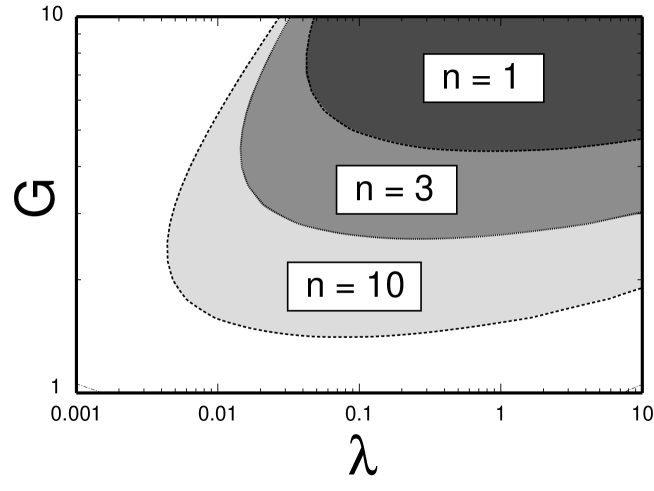
Figure 1: The allowed regions (shadowed) of the scalar self-coupling constant $\lambda$ and the Yukawa coupling constant $G$ for the Fermi ball to be stable against the fragmentation. We assume that the fermion $\Psi_{i}$ ($1\leq i\leq n$) belongs to a multiplet and the boson $\phi$ to a singlet of the internal symmetry, and that the fermion number $N_{i}$ is common to the flavor as $N_{i}=N$. The figure shows that the allowed region broadens as $n$ increases.

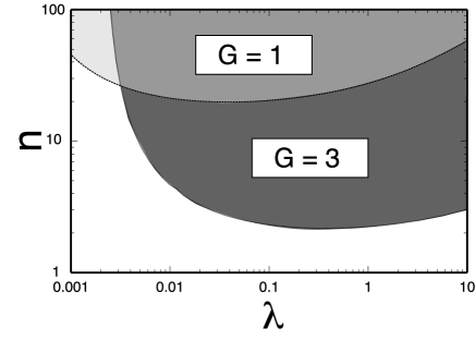
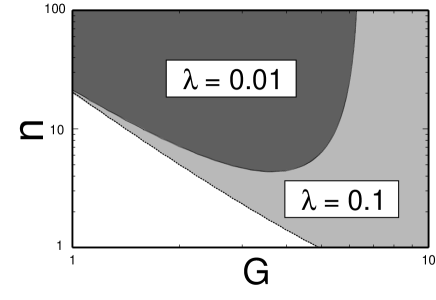
Figure 2: The allowed region (shadowed) of the scalar self-coupling constant $\lambda$ (left) and the Yukawa coupling constant $G$ (right) for the Fermi ball to be stable. The assumptions are the same as those in Figure 1. We see that the allowed regions broaden as $n$ increases.

These figures show that the allowed regions of the parameters exist for the Fermi ball to be stable against the fragmentation (the shadowed regions in the figures). We see in the figures that the allowed region broadens as the number of the flavors $n$ increases.

III CONCLUSION

We have considered a model for the Fermi ball in which the fermions with multi-flavors $\Psi_{i}$ ($1\leq i\leq n$) are coupled to the scalar field $\phi$ and the total fermion number of each $i$-th flavor is fixed as $N_{i}$. We have examined the region of the parameters for the Fermi ball to be stable against fragmentation, and how the number of the fermion flavors $n$ affects the stability.

We have considered the thin-wall Fermi ball, i.e., the radius $R$ is much larger than the wall thickness $\delta_{b}$. We have taken into account the effect due to the finite wall thickness by the perturbation expansion with respect to $\delta_{b}/R$. In the leading order thin-wall approximation, we have compared the energy of the initial state of a single Fermi ball and that of the final state of fragmented $m$ Fermi balls, with the total fermion number $N_{i}$ of each flavor $i$ being conserved, $\sum_{a=1}^{m}N_{i}^{(a)}=N_{i}$. We have found that the former is smaller than the latter and thus the Fermi ball is stable against fragmentation, except for the special case of $N_{i}^{(a)}=c^{(a)}N_{i}$ with $\sum_{a=1}^{m}c^{(a)}=1$. This situation that the Fermi ball is stable in most cases is characteristic of the case with multi-flavor of fermions, and qualitatively different from the case of a single flavor. In the special case of $N_{i}^{(a)}=c^{(a)}N_{i}$, the two states have the same energy in the leading order approximation and the next-to-leading order correction term $\delta E$ determines the stability. There we have found that the energy of the initial state is $E_{0}+{\cal C}v$ and that of the fragmented states is $E_{0}+m{\cal C}v$, where $v$ is a symmetry breaking scale and ${\cal C}$ is a coefficient dependent on the scalar self-coupling constant $\lambda$, the Yukawa coupling constant $G_{i}$ and the fermion number $N_{i}$. This tells us that even in that case the Fermi ball is stable when ${\cal C}$ takes a positive value in the parameter region of $\lambda$, $G_{i}$ and $N_{i}$.

We have considered the simplified model in which a multiplet of fermions has a common $G_{i}$ and a common $N_{i}$ for each flavor $i$. We have found that the allowed region of the parameters for the Fermi ball to be stable exists and broadens as the multiplet dimension $n$ increases.

References

• (1) A. L. Macpherson and B. A. Campbell, Phys. Lett. B347 (1995) 205.
• (2) J. R. Morris, Phys. Rev. D59 (1999) 023513.
• (3) T. D. Lee and Y. Pang, Phys. Rep. 221 (1992) 251.
• (4) For the examples of zero-mode fermions bound in the domain wall, see: G. Dvali and M. Shifman, Nucl. Phys. B504 (1997) 127 ; M. Sakamoto and M. Tachibana, Phys. Lett. B458 (1999) 231.
• (5) J. Arafune, T. Yoshida, S. Nakamura and K. Ogure, Phys. Rev. D62 (2000) 105013.
• (6) T. Yoshida, K. Ogure and J. Arafune, hep-ph/0210062, to appear in Phys. Rev. D.
• (7) K. Ogure, T. Yoshida and J. Arafune, hep-ph/0212332.