Torus structure on graphs and twisted partition functions for minimal and affine models

1 Introduction

1.1 Purpose and structure of this article

One of the purposes of our article is to present a discussion and a classification of twisted partition functions for conformal field theories associated with minimal models and affine models of type ADE, as well as some of their generalizations associated with diagrams belonging to higher Coxeter – Dynkin systems. The whole discussion is based on the quantum geometry of these diagrams. Since the graphs themselves provide the necessary combinatorial data, we shall avoid as much as possible to make any explicit use of the theory of affine Lie algebras (or of their finite dimensional counterparts). Actually, we shall not use much information coming from Conformal Field Theory, so that our presentation should be understood by readers with different backgrounds.

Many mathematical tools used in the study of the quantum geometry of graphs were introduced by A. Ocneanu (in the context of operator algebras) and later “explained” or adapted in various contexts (for instance CFT but not only) by several authors; this information is scattered in publications of very different nature. Our presentation starts from very elementary concepts and shows how one can calculate many (quantum) geometrical quantities of interest by using rather straightforward algorithms. From the data encoded in $ADE$ diagram or their generalizations, we remind the reader how the corresponding quantum geometry is related to the (twisted or not) partition functions in affine models. We then move to minimal models in particular the unitary ones, discuss the relation with graphs and give various examples (Ising, Potts and the exceptional $E_{6}$ - ${\ A_{10}}$ model). We also consider twisted ${\cal W}_{3}$ minimal models.

Our discussion of twisted partition functions for minimal models can be summarized as follows : to a pair $(G^{(1)},G^{(2)})$ of $ADE$ Dynkin diagrams one can associate six types of sesquilinear forms on the space of Virasoro characters. These forms can be interpreted, in terms of minimal models, as partition functions in boundary conformal field theory with defects. This classification rests on the possibility of introducing several “torus structures” for the two diagrams $G^{(1)}$ and $G^{(2)}$. Torus structures are parametrized by elements of a particular base in the Ocneanu algebra of quantum symmetries; a torus structure may have a single twist, two twists, or no twist at all. The interpretation of what we call torus structures in terms of defects (or twists) in a conformal field theory with boundary was proposed by V.B. Petkova and J.-B. Zuber [38]. An application of these ideas to the discussion of the different types of partition functions for minimal models was presented in the publication [34]. In general, twisted partition functions are not modular invariant, and we discuss what is left of this invariance in various cases. We also describe what happens when the $ADE$ Dynkin diagrams are replaced by members of an higher Coxeter-Dynkin system (Di Francesco – Zuber diagrams in the case of $SU(3)$).

We want this article to be almost “self contained” and we shall have therefore to remind the reader several facts or constructions that, in principle, can be found in the literature. For this reason we make here a short list of several specific results of the present paper, results that, to our knowledge, cannot be found elsewhere: the use of induction/restriction matrices to obtain all twisted partition functions (with one or two twists), the use of the multiplication table of the algebra of quantum symmetries $Oc(G)$ in order to obtain identities between toric matrices, the $12\times 12$ multiplication table of $Oc(E_{6})$, the list of toric matrices with two twists (and the corresponding partition functions) for the affine $E_{6}$ model, the behaviour of these functions with respect to the action of the modular group, a general discussion of the various types of twisted partition functions for minimal models (see however the previous footnote), several explicit examples of twisted versions of Virasoro minimal models, for instance $(A_{10}-E_{6})$ and several examples of twisted ${\cal W}_{3}$ - minimal models, for instance $({\mathcal{A}}_{4}-{\mathcal{E}}_{5})$.

Although many of the results and formulae that we mention belong to the lore of CFT (in particular affine WZW models or minimal models), we decide to adopt a presentation that uses graphs (or pairs of graphs) as primary data, so that we can avoid, as much as possible, to make use of results coming from the theory of Virasoro algebra or of affine Lie algebras; we therefore hope that the reader will find our presentation to be of independent interest.

1.2 Torus structures of Dynkin diagrams and their generalizations

Here is a brief presentation of the various structures that will be discussed later in this paper.

To a given Dynkin diagram $G$ (or to a member of an higher Coxeter-Dynkin system) one associates the complex vector space (also called $G$) spanned by the vertices of this diagram. In some cases (in particular for all diagrams belonging to the $A$ series), this vector space $G$ possesses an associative (and commutative) multiplication law with positive integral structure constants and it is called the “graph algebra”; one also says that the diagram (or the corresponding vector space) admits “self fusion”. In the case of ADE diagrams, whether or not the vector space of the diagram $G$ (with Coxeter number $\kappa$) admits self fusion, it is anyway a module over the graph algebra of the diagram $A_{\kappa-1}$, with the same Coxeter number. More generally, i.e., for higher Coxeter – Dynkin systems, the vector space $G$ is a module over a particular graph algebra that we call $\mathcal{A}(G)$.

Following Ocneanu [29], to every diagram $G$ (with or without self - fusion) belonging to a Coxeter-Dynkin system, one can associate a bi-algebra $\mathcal{B}G$. By using a particular scalar product, it is easier to think that $\mathcal{B}G$ is actually a di-algebra (a vector space with two compatible associative algebra structures). There are two – usually distinct – block decompositions for this di-algebra (see later). Blocks of the first type are labelled by points of a graph that we call $\mathcal{A}(G)$. Blocks of the second type are labelled by points of a graph that we call $Oc(G)$. The vector spaces spanned by the vertices of these two graphs are themselves endowed with natural associative algebra structures that we denote by the same symbol as the graphs themselves. The algebra $\mathcal{A}(G)$, coincides, for $G$ of type ADE, with the graph algebra of a particular member of the $A$ family, and it is a commutative algebra, but $Oc(G)$, also called “algebra of quantum symmetries” of $G$ is not always commutative.

The algebra of quantum symmetries $Oc(G)$, like the vector space $G$ itself, comes with a particular basis and its multiplicative structure is encoded by a graph called $Oc(G)$ whose vertices are in one to one correspondence with the distinguished generators. In the particular case where $G$ is a member of the $A$ series, the algebras $\mathcal{A}(G)$, $Oc(G)$ and $G$ coincide.

We call $i,j,\ldots$ the vertices of $\mathcal{A}(G)$, $a,b,\ldots$ the vertices of $G$ and $x,y,\ldots$ the vertices of $Oc(G)$. Remember that “vertices” should be thought of as elements of the various (distinguished) basis for the corresponding vector spaces. We denote by $\underline{0}$ the identity of $Oc(G)$. The vector space $G$ is a module over $\mathcal{A}(G)$ , and the algebra $Oc(G)$ is a bi-module over $\mathcal{A}(G)$; this bi-module structure is encoded by a set of matrices (toric matrices) defined as follow:

$$i.x.j=\Sigma_{y}(W_{x,y})_{ij}y$$

A torus structure for the diagram $G$ is (by definition) specified by the choice of a matrix $W_{x,y}$. If the dimension of $Oc(G)$ is $s$, the number of independent toric structures is a priori $s^{2}$, but very often we may have degeneracies, in the sense that we may obtain the same toric matrix for different choices of the pair $(x,y)$.

It is convenient to introduce the following terminology: the undeformed torus structure corresponds to the choice of the matrix $W_{\underline{0},\underline{0}}$, a deformed torus structure along one “defect line” specified by $x$ corresponds to the choice of the matrix $W_{\underline{0},x}$ (or $W_{x,\underline{0}}$) and a deformed torus structure along two defect lines specified by $x$ and $y$ corresponds to the choice of the matrix $W_{x,y}$. It is convenient to set $W_{x}\doteq W_{x,\underline{0}}$ and in particular $W_{0}\doteq W_{\underline{0},\underline{0}}$.

1.3 Frustrated (or twisted) partition functions for affine models

1.3.1 Twisted partition functions for affine models

For affine models characterized by the affine Kac - Moody algebra of type $\widehat{su}(2)$ (chiral algebra), the classification of modular invariant partition functions is well known [7], and was shown to be in one-to-one correspondence with $ADE$ Dynkin diagrams. More recently [29], it was shown that if the theory is associated with the Dynkin diagram $G$, its modular invariant partition function is given by $Z_{0}=\overline{\chi}W_{\underline{0},\underline{0}}\chi$ where $\chi$ is a vector of the complex vector space $\mathbb{C}^{n}$ and $W_{\underline{0},\underline{0}}$ is the toric matrix associated with the origin of the Ocneanu graph of the diagram $G$. This characterization of partition functions uses only the (quantum) geometry of the diagram $G$ and does not refer to the theory of affine algebras; in this approach, for instance, the fact that $\chi$ could be interpreted as a character of an affine Lie algebra is not used; in particular, modular invariance is implemented by finite dimensional matrices representing $SL(2,\mathbb{Z})$.

As shown in [37] and [38], the other partition functions of type $Z_{x}=\overline{\chi}W_{\underline{0},x}\chi$ , or more generally $Z_{x,y}=\overline{\chi}W_{x,y}\chi$, can be interpreted as twisted partition functions in a boundary conformal field theory (boundary “of type” $G$), in the presence of defect lines of type $x$ and $y$. A simple algorithm for the calculation of the matrices $W_{\underline{0},x}$ was presented in [9] (where the example of $E_{6}$ was chosen) and explicit results for all $ADE$ cases are given in [11] (see also [12] for generalizations to higher Coxeter-Dynkin systems). The definition of matrices $W_{x,y}$ in [38] looks different from ours (we use the description of the bimodule structure of $Oc(G)$ over $A_{\kappa-1}$) but it can be shown to be equivalent (see our comment in section 4.2). The matrix $W_{0}\doteq W_{0,0}$ is a modular invariant: it commutes with the generators $S$ and $T$, representing $SL(2,\mathbb{Z})$ in the vector space spanned by the vertices of the graph $\mathcal{A}_{\kappa-1}$. The corresponding sesquilinear form is the modular invariant partition function. The other matrices $W_{x,y}$ are associated with partition functions that are not modular invariant.

For affine models characterized by the affine Kac - Moody algebra of type $\widehat{su}(N)$, the story is very similar. Here $\chi$ is still a vector of the complex vector space $\mathbb{C}^{n}$ but $n$ now denotes the cardinality of the set of vertices of a graph $\mathcal{A}(G)$ generalizing the $A_{\kappa-1}$ Dynkin diagram. In the case of $SU(3)$ for instance, the $ADE$ diagrams are replaced by the Di Francesco - Zuber diagrams, but we can again define the bialgebra $\mathcal{B}G$ and the two related associative algebras $\mathcal{A}(G)$ and $Oc(G)$. Torus structures on these diagrams and corresponding twisted partition functions are defined as before.

1.3.2 Twisted partition functions for minimal models and their higher analogues

Minimal models

It has been known for quite a while (see for instance the book [18]) that the classification of modular invariant partition functions for minimal models, unitary or not, also follows a kind of $ADE$ classification, in the sense that every partition function describing a minimal model can be associated with a pair of Dynkin diagrams $(G^{(1)},G^{(2)})$. In our set-up, this affirmation can be precisely formulated as follows: the partition function of a minimal model of type $(G^{(1)},G^{(2)})$ can be obtained as the sesquilinear form associated with the matrix $W_{\underline{0},\underline{0}}^{(1)}\otimes W_{\underline{0},\underline{0}}^{(2)}$ where these two matrices respectively describe the undeformed torus structures of diagrams $G^{(1)}$ and $G^{(2)}$. It is also well known that the obtained minimal model is unitary if and only if the Coxeter numbers $\kappa_{1}$ and $\kappa_{2}$ of the two diagrams $G^{(1)}$ and $G^{(2)}$ just differ by one unit. The usual situation for minimal models corresponds therefore to the choice of the two trivial torus structures for the graphs $G^{(1)}$ and $G^{(2)}$; the possibility of replacing these two torus structures by more general ones (i.e., matrices $W_{\underline{0},\underline{0}}^{(1)}$ and $W_{\underline{0},\underline{0}}^{(2)}$ by matrices $W_{x_{1},y_{1}}^{(1)}$ and $W_{x_{2},y_{2}}^{(2)}$) leads to a natural classification of twisted partition functions for minimal models.

Analogues of minimal models for general Coxeter-Dynkin systems

The general case of minimal models corresponds to the choice of two graphs of type $SU(2)$ (i.e., two arbitrary Dynkin diagrams of type ADE) but one can also replace the two $ADE$ diagrams $G^{(1)}$ and $G^{(2)}$ by members of an higher Coxeter-Dynkin system (for example the Di Francesco - Zuber diagrams of type $SU(3)$) and obtain in this way similar classifications. Here the notion of “minimal model” is generalized and the corresponding partition functions, twisted or not, can be interpreted in terms of minimal models for ${\mathcal{W}}_{n}$ algebras (in particular ${\mathcal{W}}_{3}$ for the Di Francesco - Zuber diagrams).

1.4 A brief historical section

Here we make a long story short and gather only a few references. Many others can be found by looking at the quoted material. Apologies for omissions.

The study of quantum geometry of $ADE$ graphs was, at the beginning, presented as a nice example illustrating the general theory of “paragroups” and “Ocneanu cells” [27]. This class of examples and its generalizations turned out to be very rich. Much of the theory was developed by A. Ocneanu himself and described (sometimes in a rather allusive way) at several meetings and conferences during the years $95-2000$ ( for instance [28]). As far as we know, the first published material on this theory is [29].

From the physical side, many relations existing between $ADE$ graphs and physics (models of statistical mechanics) had been already observed and investigated by V. Pasquier in his thesis (see [32]). A classification of modular invariant partition functions for conformal field theories of $SU(2)$ type was obtained at the same time, i.e., at the end of the eighties, by [7] in a celebrated paper. Later, T. Gannon (and collaborators) could obtain ([21]) similar results for conformal field theories based on more general affine Kac – Moody algebras.

Di Francesco and Zuber made the crucial observation [16] that the $SU(3)$ classification could be related to a family of particular graphs (that we call the Di Francesco – Zuber diagrams), in a way similar to the relation existing between the $SU(2)$ classification and the $ADE$ Dynkin diagrams. Several precisions concerning this classification were brought by A. Ocneanu at the Bariloche school ([30], see also the lectures of J.-B. Zuber and D. Evans at the same school).

After the unpublished work by Ocneanu concerning the $ADE$ themselves, it was more or less clear that the existence of modular invariant partition functions associated with these diagrams (or their generalizations) was only the tip of a theoretical iceberg. For instance, from the existence of several toric structures on $ADE$ diagrams, it was clear that the modular invariant partition function was only describing a particular point of $Oc(G)$, and that other “interesting” partition functions claiming for a physical interpretation existed in the theory. A simple algorithm allowing one to obtain the toric matrices $W_{x,\underline{0}}$ was explained in [9], following the example of $E_{6}$, and, as already mentioned, a physical interpretation of the $W_{x,y}$ in terms of conformal field theory with a boundary and defects lines was given in [38]. Using the techniques explained in [9], a systematic study of all $ADE$ cases was performed in [11] and several interesting cases belonging to the $SU(3)$ family were analyzed in [12]. In [20], several properties of the twisted partition functions were interpreted in terms of bimodules for Frobenius algebras. More recently (see [35] and footnote 1), it was shown how to build a lattice realization of these models.

2 Quantum geometry on $ADE$ diagrams and their generalizations

2.1 From the classical to the quantum situation (in a nutshell)

Classical situation.

Representation theory of Lie groups ($SU(2)$, $SU(3)$, etc) and their subgroups can be encoded by graphs. These graphs tell us how to decompose the representations obtained by tensor multiplying irreducible representations (irreps); actually it is enough to know what happens when one tensor multiplies some irrep by the fundamental representations. Representation theory of $SU(2)$ is encoded, in this way, by the graph $A_{\infty}$ (it describes the coupling of an arbitrary spin with a spin $1/2$ ). Representation theory of $SU(3)$ is characterized by two generalized $\mathcal{A}_{\infty}$ diagrams differing only by orientation (multiplication by the fundamentals $3=(1,0)$ of $\overline{3}=(0,1)$). Such a graph defines an associative algebra (the “graph algebra”) which is the the Grothendieck ring spanned by the irreducible characters of the group. Notice that the graph algebra of a subgroup is a module over the graph algebra of the group and that the structure constants characterizing these associative algebras, or modules, are positive integers.

Quantum situation.

In the case of $SU(2)$, truncating the diagram $A_{\infty}$ leads to the usual $A_{n}$ Dynkin diagrams. In the case of $SU(3)$, truncating one of the two diagrams $\mathcal{A}_{\infty}$ leads to the Di Francesco – Zuber diagrams of type $\mathcal{A}$. This can be generalized to $SU(N)$ [39]. The vector space spanned by the vertices of any $\mathcal{A}$ diagram, for a given $SU(N)$ system, always possess a $\mathbb{Z}_{N}$ grading (called $N$ -ality). For instance, in the case of the usual $A_{n}$ Dynkin diagrams, vertices are either ”even” or ”odd”. All these graphs “of type $\mathcal{A}$” have self - fusion (an associative multiplication law with positive integral structure constants), but they are not the only ones enjoying this property. The obtained graph algebras are associative and commutative algebras with a particular basis, they are denoted by the same symbol as the graph itself. For a given $N$ (the choice of $SU(N)$), the first task is to determine all those diagrams which simultaneously admit $N$-ality, generate a module (with integral structure constants) over some associative algebras of type $\mathcal{A}$ and also admit self-fusion. The next task is to identify all those diagrams (with $N$-ality) which do not necessarily enjoy self-fusion, but which nevertheless generate a module (with integral structure constants) over one of the algebras defined by the previous family. A list of requirements that a given diagram should obey in order to be a member of some “generalized Coxeter - Dynkin system” was given in reference [39], but as mentioned by A. Ocneanu in [30] (see also [31]), this list was not complete, in the sense that a local condition of cohomological nature should also be imposed on its set of “cells”; this is not discussed here.

2.2 The classical and quantum systems of diagrams for $SU(2)$ and $SU(3)$

The classical $\mathbf{SU(2)}$ system.

Choose a finite subgroup of $SU(2)$, i.e., one of the so-called binary polyhedral groups. The fundamental representation is again $2$ dimensional and the multiplication of any of its irreps by the fundamental is encoded by the corresponding diagram of tensorisation, which, for the binary groups of symmetries of platonic bodies coïncides with the affine exceptional Dynkin diagrams $E_{6}^{(1)}$, $E_{7}^{(1)}$, $E_{8}^{(1)}$ (McKay correspondence, [26]). The vector space generated by the set of irreducible representations of such a subgroup is a module over the algebra generated by the set of irreps of $SU(2)$ (reduce irreps from the group $SU(2)$ to its subgroup and use tensor multiplication of representations). In diagrammatic parlance, we may say that affine $ADE$ diagrams are modules over the $A_{\infty}$ diagram. Irreps of a binary polyhedral group can also be tensor multiplied and decomposed into irreps (with positive integral structure constants). In other words : affine $ADE$ diagrams have self fusion. In particular one of the vertices $\sigma_{j}$ acts as the unit, we call it $\sigma_{0}$. For each of these diagrams, call $G_{1}$ the adjacency matrix; its highest eigenvalue $\beta$ (called the Perron - Frobenius norm of the diagram) is equal to $2$ in all cases and it coïncides with the dimension of the fundamental representation. For a given diagram, dimensions of the irreps are given by components of the (unique) normalized eigenvector corresponding to $\beta$ (it is normalized to $1$ at the unit point $\sigma_{0}$). The table of characters $S$ happens to be equal to the matrix of eigenvectors (properly normalized) of $G_{1}$. This is a way to express the general McKay correspondence in the case of $SU(2)$.

The quantum $\mathbf{SU(2)}$ system.

Now we move to the quantum case and replace the $A_{\infty}$ diagram by $A_{n}$ diagrams seen as truncated $A_{\infty}$ diagrams. These diagrams $A_{n}$ have self - fusion. The next task is to determine those diagrams (with bi-ality) that generate modules over the $A_{n}$ : we get the $A$, $D$ and $E$ diagrams. For example, $E_{6}$ is an $A_{11}$ module, $E_{7}$ an $A_{17}$ module, and $E_{8}$ an $A_{29}$ module. Some of them have self-fusion ($A_{n}$, $D_{eve}$, $E_{6}$, $E_{8}$), others don’t ($D_{odd}$, $E_{7}$). A diagram $D_{eve}$ actually determines a two-parameters family of associative structures, but only two of them have structure constants which are positive integers (self fusion); these two structures can be identified when we permute the two end points of the $D_{even}$ fork; when such a phenomenon appears, the algebra of quantum symmetries $Oc(G)$, to which we shall return later, appears to be non commutative.

The norm of a diagram $G$ is found to be $\beta=2\cos\frac{2\pi}{\kappa}$, where $\kappa=n+1$ if $G=A_{n}$ or when $G$ is a module over $A_{n}$. Note that $1<\beta<2$ (see also [23]). The quantum dimensions $qdim_{a}$ of the vertices of $G$ are obtained or defined as the components of the normalized Perron Frobenius eigenvector (which corresponds to the eigenvalue $\beta$). For every $ADE$ diagram, i.e., for every member $G$ of the system that we may call “the $SU(2)$ Coxeter-Dynkin system”, the integer $\kappa$ is called the Coxeter number of the diagram. All these diagrams (with or without self - fusion) can also be labelled by an integer $k$, called the level of the diagram and defined by $k=\kappa-2$. A description of the ADE diagrams in terms of representations of quantum subgroups (a quantum analogue of the McKay correspondance) was discussed by [25] in the framework of modular categories.

The classical $\mathbf{SU(3)}$ system.

Representation theory for finite subgroups of $SU(3)$ is fully characterized by a family of diagrams that have self – fusion and generate modules over the graph algebra of the generalized $\mathcal{A}_{\infty}$ diagram of $SU(3)$. All of these diagrams have a norm equal to $3$.

The quantum $\mathbf{SU(3)}$ system.

Now we move to the quantum and replace $\mathcal{A}_{\infty}$ by $\mathcal{A}_{k}$ (truncated $A_{\infty}$ diagrams). These $\mathcal{A}_{k}$ have self-fusion. The next task is to determine those diagrams (with tri-ality) that are modules over the $\mathcal{A}_{k}$ : we get the Di Francesco – Zuber diagrams. Some of them have self-fusion and others don’t. The system contains in particular the $\mathcal{A}$ series and a finite number of “genuine exceptional” cases ($\mathcal{E}_{5}$, $\mathcal{E}_{9}$ and $\mathcal{E}_{21}$). The other diagrams of the system are obtained as orbifolds of the genuine diagrams (exceptional or not) and as twists or conjugates (sometimes both) of the genuine diagrams and of their orbifolds. See references [16], [39] [30], [40]. All of them have a norm $\beta$ equal to $1+2\cos\left(\frac{2\pi}{\kappa}\right)$. Note that $2<\beta<3$. This again defines an integer $\kappa$ called the “generalized Coxeter number” or “altitude” (like in [16]). The level $k$ of a diagram belonging to this family is defined by the relation $k\doteq\kappa-3$. The truncated $\mathcal{A}_{\infty}$ diagrams that we call $\mathcal{A}_{k}$ are of level $k$ (see the footnote in the next subsection). Even when it exists, the determination of the graph algebra of a given diagram is not always unique; a phenomenon similar to what happens for the $D_{even}$ diagrams (see a previous remark) occurs for instance in the case of the ${\mathcal{E}}_{9}$ diagram of the $SU(3)$ system.

2.3 General notations and characteristic numbers for generalized Coxeter-Dynkin diagrams

The classical representation theory of $SU(N)$ can be encoded by a set of $N-1$ diagrams (with oriented edges and infinitely many vertices) generalizing the $A_{\infty}$ diagram of $SU(2)$; there is one such oriented diagram for each fundamental representation. For definiteness, we choose the basic representation of $SU(N)$; its Young tableau is given by a single box. A given system of diagrams is then labelled by an integer $N$, it has the same value for all diagrams of a system. For $ADE$ Dynkin diagrams, $N=2$, the (dual) Coxeter number of $SU(2)$. For Di Francesco - Zuber diagrams, $N=3$, the (dual) Coxeter number of $SU(3)$. The generalized Coxeter number (altitude) of a diagram $G$ is called $\kappa$ in our paper, it can be defined directly from the norm $\beta$ of $G$; for usual Dynkin diagrams, altitude is the usual dual Coxeter number. It is useful to define the root of unity $\mathbf{q}\doteq exp{\frac{i\pi}{\kappa}}$, so that $\mathbf{q}^{2\kappa}=1$. The level $k$ of a given diagram belonging to a given system of type $SU(N)$ is defined by the relation $k\doteq\kappa-N$. More generally, one could probably define generalized Coxeter-Dynkin systems for any Lie group (the case $SU(2)$ corresponding to the $ADE$ system), but such a theory remains to be investigated.

As we know, for a given system, members of the $\mathcal{A}$ family (call them $\mathcal{A}_{k}$, with $k$ standing for the level) are obtained as truncated $\mathcal{A}_{\infty}$ diagrams. They can be related to a particular category of representations of quantum groups at roots of unity, but we shall not discuss this aspect here.

A diagram $G$ of level $k$ belonging to such a generalized system is always such that the vector space spanned by the set of its $m$ vertices is a module over the member $\mathcal{A}_{k}$ of the $\mathcal{A}$ family with the same level (the number of vertices of this corresponding diagram of type $\mathcal{A}$ will be called $n$, so $m=n$ when $G$ is of type $A$. Notice that $n=k+1$ for usual $A_{n}=\mathcal{A}_{k}$ Dynkin diagrams, but $n=(k+1)(k+2)/2$ for Di Francesco – Zuber diagrams of type $\mathcal{A}_{k}$.

The list of exponents $\{r\}$ of a graph $G$ of type $ADE$ can be defined directly from the table of eigenvalues of the adjacency matrix $G_{1}$ of $G$: these eigenvalues are of the form $2Cos(r\pi/\kappa)$. For instance, in the case of $E_{6}$, from the list of eigenvalues,

$$\{2Cos(\pi/12),2Cos(4\pi/12),2Cos(5\pi/12),2Cos(7\pi/12),2Cos(8\pi/12),2Cos(11\pi/12)\}$$

we read the exponents $\{1,4,5,7,8,11\}$. Notice that exponents also refer to particular vertices of the corresponding diagram of type $\mathcal{A}$ with the same Coxeter number (for $E_{6}$, see the circled vertices on figure 3, and remember that our indices for labelling vertices are shifted by $1$). The list of exponents $\{r=(r_{1},r_{2})\}$ of a graph $G$ belonging to a generalized system can also be defined directly from the adjacency matrix $G_{1}$ of $G$. For Di Francesco - Zuber diagrams (ie the $SU(3)$ system), they can be read from the following general formula giving the eigenvalues of $G_{1}$ ([16]) ${(1+e^{\frac{2i\pi r_{1}}{\kappa}}+e^{\frac{2i\pi(r_{1}+r_{2})}{\kappa}})}/{e^{\frac{2i\pi(2r_{1}+r_{2})}{3\kappa}}}$. For instance, the exponents of ${\mathcal{E}}_{5}$ are

$$\{(1,1),(3,3),(1,3),(4,3),(3,1),(3,4),(3,2),(1,6),(4,1),(1,4),(2,3),(6,1)\}$$

Here again, exponents refer to particular vertices of the corresponding diagram of type $\mathcal{A}$ with the same Coxeter number and remember that indices labelling vertices are usually shifted by $(1,1)$. Exponents appear in the expression giving the corresponding modular invariant partition function (see the examples of ${E}_{6}$ or of ${\mathcal{E}}_{5}$ in sections 3.1.5 and 3.2) and in the usual (or generalized) Rocha-Cariddi formulae.

2.4 Paths, essential paths, the bi-algebra $\mathcal{B}G$ and the algebra $Oc(G)$ of quantum symmetries

We then move from the geometry of the “space” $G$ to the geometry of the paths on $G$, a procedure quite common in quantum physics! Paths on $G$ generate a vector space $Paths$ which comes with a grading: paths of homogeneous grade are associated with Young diagrams of SU(N). In the case of $SU(2)$ this grading is just an integer (to be thought of as a length, a Young frame with a single row, or as a point of $A_{n}\equiv\mathcal{A}_{k=n-1}$).

What turns out to be most interesting is a particular vector subspace of $Paths$ whose elements are called “essential paths” (we refer to [29], [9], see also [10] for a definition). The space of essential paths $EssPaths$ is itself graded in the same way as $Paths$ and one may consider the graded algebra of endomorphisms of essential paths $\mathcal{B}G\doteq End_{\sharp}(EssPaths)=\bigoplus_{j=0,r-1}End(EssPaths^{j})$.

By using the fact that paths on the chosen diagram can be concatenated , one may define another multiplicative (associative) structure on the vector space $\mathcal{B}G$ (see [29] for a definition). This leads to a di-algebra $\mathcal{B}G$ which turns out to be semi-simple for both structures, but existence of a scalar product allows one to transmute one of the multiplications into a co-multiplication compatible with the other structure and one obtains in this way a bi-algebra. This bi-algebra is sometimes called, by A. Ocneanu “Algebra of double triangles” (DTA), a terminology coming from the graphical representation of the corresponding elementary matrices by diffusion graphs or, dually, as double triangles.

For these two associative laws on the same space, that we may call “composition law” and “convolution law” (or “vertical law” and “horizontal law”), there are two — usually distinct — block decompositions for $\mathcal{\ B}G$ (ideals corresponding to simple blocks). The first type of blocks, labelled by $j$, corresponds to the grading associated with points $\sigma_{j}$ of $\mathcal{\ A}_{k}$, i.e., in the case of $SU(2)$, to the lengths of the paths, and, more generally, to Young diagrams of $SU(N)$); interpretation of this first block structure is therefore clear from the definition of $\mathcal{B}G$ as sum of algebras of endomorphisms. The second block decomposition can be interpreted as follows: $ADE$ diagrams (or their $SU(N)$ generalizations) may have classical symmetries, for instance, all $A_{n}$ diagrams have an obvious $\mathbb{Z}_{2}$ symmetry; these classical symmetries (action of a finite group on vertices) can be promoted to the level of paths in an obvious way and therefore lead to particular endomorphisms of $EssPaths$; but there are more “quantum symmetries” acting on the space of essential paths than classical symmetries: irreducible quantum symmetries (call them $x$) are precisely associated with the blocks of $\mathcal{B}G$ for the second multiplication. We call $Oc(G)$ the algebra spanned by the minimal central projectors associated with the later blocks, using the first multiplicative structure. $Oc(G)$ is called the “algebra of quantum symmetries”. In all cases it is an associative algebra with two generators (called “left” and “right” generators) and the Cayley graph of multiplication by these two generators, called the “Ocneanu graph of $G$” is also denoted by $Oc(G)$. The linear span of these generators are called left and right chiral parts, and their intersection is called “ambichiral”.

The number of (simple) blocks of ${\cal B}G$ for its first multiplication, is $n$ (the number of points of the corresponding ${\cal A}$ diagram); dimension of these blocks will be called $d_{j},j=1\ldots n$. The number of (simple) blocks of ${\cal B}G$ for its second multiplication, will be called $s$ (the number of points of the corresponding Ocneanu diagram); dimension of these blocks will be called $d_{x},x=1\ldots s$. Existence of two block decompositions for the same underlying vector space $\mathcal{B}G$ leads obviously to the number-theoretical identity (quadratic sum rule): $\sum_{i=1,n}d_{i}^{2}=\sum_{x=1,s}d_{x}^{2}$. In all cases explicitly studied so far, an unexpected linear sum rule also holds (in some cases one has to introduce a natural correction factor).

The direct determination of the algebra $Oc(G)$, using the definition provided by A. Ocneanu, is not an easy task, and the corresponding graphs were first known (published) for the $SU(2)$ Coxeter-Dynkin system [29]. This algebra is not always commutative. One of the purposes of [9] and [11], besides the calculation of the toric matrices, was actually to give an algebraic construction providing a realization of the algebra $Oc(G)$ in terms of graph algebras associated with appropriate Dynkin diagrams. In many relatively easy cases where $G$ admits self-fusion and is also such that $Oc(G)$ is commutative, the algebra of quantum symmetries is isomorphic with $G\otimes_{J}G$, where $J$ is a particular subalgebra of the graph algebra of $G$; the tensor product sign, taken “above $J$”, means that we identify $au\otimes b$ and $a\otimes ub$ whenever $u\in J\subset G$. In those easy cases, and as shown in [12], the subalgebra $J$ can be determined from the modular properties of the graph $G$; we shall remind the reader how this is done in a later section. Paradoxically, for Dynkin diagrams, and besides the $A_{n}$ themselves, the “simple” cases happen to be those where $G$ is an exceptional diagram equal to $E_{6}$ or $E_{8}$. We refer to [11] for a discussion of all $ADE$ cases and [12] for a discussion of a number of cases belonging to the Di Francesco - Zuber system.

2.5 The matrices $N_{i}$, $F_{i}$, $G_{a}$, $E_{a}$, $S_{x}$ and $W_{x,y}$

2.5.1 Fusion matrices: the $N_{i}$’s

Fusion matrices are defined for $\mathcal{A}_{k}$ diagrams. They are square matrices of dimension $n\times n$ called $N_{i}$. They are associated with the vertices $\tau_{i}$, with $i\in\{0,\ldots,n-1\}$, and provide a faithful representation of the graph algebra. Here $i$ is actually a multi-index referring to a Young frame of $SU(N)$ and the cardinality of the indexing set is $n$. When the Young frame refers to a fundamental representation (only one column), this fusion matrix is the adjacency matrix of the corresponding oriented diagram. Other matrices $N_{i}$ are obtained from the fundamental ones by applying the particular recurrence relation specific to $SU(N)$. Example: in the case of $SU(2)$, each Young diagram is an horizontal string of boxes and is characterized by its length; the matrix $N_{1}$ is the adjacency matrix of $\mathcal{A}_{k}=A_{n=k+1}$ and $N_{0}$ is the unit; the recurrence relation (coupling of spins) is

$$N_{i+1}=N_{1}N_{i}-N_{i-1}$$

Matrices $N_{i}$ have indices $(j,k)$ referring to vertices of $\mathcal{A}_{k}$. These matrices generate a (commutative) associative algebra isomorphic with the algebra of the given $\mathcal{A}$ diagram. The indices $i,j$ runs from $0$ to $n-1$ but we shall sometimes use indices $r=i+1,s=j+1$ running from $1$ to $n$. In the case of $SU(3)$, the index $j$ labelling vertices $\tau_{j}$ of the ${\mathcal{A}}_{\kappa}$ diagram is a pair $(j_{1},j_{2})$, with $j_{1},j_{2}\geq 0$ and $j_{1}+j_{2}\leq k$. The identity is $N_{0,0}$ and the matrix $N_{1,0}$ denotes the adjacency matrix of the (oriented) diagram $G$. The recurrence formula reads

$$\begin{array}[]{lcll}N_{j_{1},j_{2}}&=&0&{\text{if}\,j_{1}<0\;\,\text{or}\,j_{2}<0}\\ N_{j_{1},0}&=&N_{1,0}N_{j_{1}-1,0}-N_{j_{1}-2,1}&{}\\ N_{j_{1},j_{2}}&=&N_{1,0}N_{j_{1}-1,j_{2}}-N_{j_{1}-1,j_{2}-1}-N_{j_{1}-2,j_{2}+1}&{\text{if}\,j_{2}\neq 0}\\ N_{0,j_{1}}&=&N_{j_{1},0}^{T}&{}\end{array}$$

2.5.2 Fused adjacency matrices: the $F_{i}$’s

The module property (external multiplication) of the vector space associated with a diagram $G$, of level $k$ and possessing $m$ vertices, with respect to the action of the algebra $\mathcal{A}_{k}$ is encoded by a set of $n$ matrices $F_{i},{i=0\ldots n-1}$, of dimension $m\times m$, sometimes called “fused graph matrices” (a somehow misleading terminology!): $\tau_{i}\sigma_{a}=\sum_{b}(F_{i})_{ab}\sigma_{b}$.

If $G$ is of type $\mathcal{A}$, we shave $n=m$, $F_{i}=N_{i}$ and we are done. More generally, call $F_{0}$ the unit matrix of dimension $m\times m$, and $F_{1}$ the adjacency matrix of $G$. For usual $ADE$ diagrams, each edge carries both orientations and $F_{1}$ is symmetric; for generalized diagrams, this is not so. Other matrices $F_{i}$ are then obtained by imposing the same recurrence relation as for the fusion matrices. Matrices $F_{i}$ have indices $(a,b)$ referring to vertices of $G$; they characterize $G$ as a module over the corresponding $\mathcal{A}$ graph. They are also in one to one correspondence with the minimal central projectors diagonalizing one of the two associative structures of the di-algebra $\mathcal{B}G$, in other words they characterize the corresponding blocks and give their dimensions $d_{i}=\sum_{a,b}(F_{i})_{a,b}$.

In the case of $SU(3)$ diagrams, remember that indices $j$ are pairs $(j_{1},j_{2})$ and that fused adjacency matrices $F_{j}$, associated with any graph $G$ of a given level, are determined by the same recurrence relations as for matrices $N_{i}=N_{j_{1},j_{2}}$ associated with the graph ${\mathcal{A}}$ of the same level; only the seed is different: $F_{1}\doteq G_{1}$, the adjacency matrix of $G$.

2.5.3 Graph matrices: the $G_{a}$’s

The diagram $G$ sometimes admits self-fusion. In those cases, the $m$ linear generators $\sigma_{a}$ of $G$ ($a$ runs from $0$ to $m-1$) are represented by $m$ commuting matrices $G_{a}$ of dimension $m\times m$ spanning a faithful representation of the graph algebra. We call $G_{0}\doteq F_{0}$, $G_{1}\doteq F_{1}$ and more generally $G_{a}$ the set of matrices (one for each vertex of $G$) representing faithfully the multiplication of vertices. Warning: with the exception of $F_{0}$ and $F_{1}$, the matrices $F_{i}$ and $G_{a}$ are distinct (in the case of $\mathcal{A}$ diagrams, of course, they are identical).

2.5.4 Essential matrices: the $E_{a}$’s

By definition, the $m$ essential matrices $E_{a}$ are rectangular matrices of dimension $n\times m$ defined by setting, for every vertex $a$ of $G$, $(E_{a})_{i,b}\doteq(F_{i})_{a,b}$. These are rectangular matrices of dimension $(n,m)$. Matrices $E_{a}$ display “visually” the structure of essential paths emanating from a vertex $a$ on the diagram $G$. One can check that, for graphs with self fusion, $E_{a}=E_{0}G_{a}$. The particular matrix $E_{0}$ is usually called “intertwiner”, in the statistical physics literature.

As we know, vertices of the diagram $G$ should be thought of as an analogue of irreducible representations for a subgroup of a group; the irreducible representations of the bigger group are themselves represented by vertices of the corresponding $A$ graph. In this analogy, the first column of each matrix $F_{i}$ would describe the branching rule of $\tau_{i}$ with respect to the chosen subgroup (restriction mechanism). In the same way, the columns of the particular essential matrix $E_{0}$ would describe the induction mechanism: the non-zero matrix elements of the column labelled by $\sigma_{b}$ tell us what are those representations $\tau_{i}$ that contain $\sigma_{b}$ in their decomposition (for the branching $A\rightarrow G$).

2.5.5 Matrices for $Oc(G)$

Since we have a di-algebra $\mathcal{B}G$ we have also a set of matrices $S_{x}$ which characterize the blocks of the other associative structure (one for each point of the Ocneanu graph). In “simple cases”, like $E_{6}$ or $E_{8}$, the matrix $S_{x}$ associated with the vertex $x=a\otimes_{J}b$ of the Ocneanu graph is simply equal to the product $G_{a}G_{b}$. The dimension $d_{x}$ of the block $x$ is obtained by summing the matrix elements of $S_{x}$.

2.5.6 Toric matrices and generalized toric matrices: the $W_{x}$ and $W_{x,y}$

We know that $\mathcal{A}_{k}$ acts on $G$, but $\mathcal{A}_{k}$ also acts (from both sides) on $Oc(G)$. In general $Oc(G)$ is an $\mathcal{A}_{k}$ bimodule and the action is encoded as follows: $\tau_{i}\,x\,\tau_{j}=\sum_{y\in Oc(G)}(W_{xy})_{j}^{i}\;y$, with $x,y\in Oc(G)$ and $\tau_{i},\tau_{j}\in\mathcal{A}_{k}$. In general, one obtains $s\times s=s^{2}$ matrices $W_{xy}$ of dimension $s\times s$, (many of them may happen to be equal). In particular one obtains the $s$ matrices $W_{x}\doteq W_{x0}$ and the matrix $W_{0}=W_{00}$ associated with the origin of the Ocneanu graph. Practically, once we have the $m$ rectangular matrices $E_{a}$, of dimension $n\times m$, we first replace by $0$ all the matrix elements of the columns labelled by vertices $b$ that do not belong to the subset $J$ of the graph $G$, call $E_{a}^{red}$ these “reduced” matrices and obtain, for each point $x=a\stackrel{{\scriptstyle\cdot}}{{\otimes}}b$ of the Ocneanu graph $Oc(G)$, a “toric matrix” $W_{x}=E_{a}\,(E_{b}^{red})^{T}$, of dimension $n\times n$.

We will explain in section 3.1.5 how to generalize the previous method to obtain all the toric matrices $W_{x,y}$ (“first algorithm”). Actually, the $W_{x,y}$ can also be obtained from the $W_{x}$, determined as above, by working out the multiplication table of $Oc(G)$ (this is our “second algorithm”). All we have to do is to decompose the product $x\times y$ on the basis generators: if $x.y=\Sigma_{z}C_{x,y}^{z}z$ with $x,y,z\in Oc(G)$ then $W_{x,y}=\Sigma_{z}C_{x,y}^{z}W_{0,z}$. This can be seen as a compatibility equation; indeed, the action of ${\cal A}_{k}$ is central, so $\tau_{i}.x.\tau_{j}=x.\tau_{i}.\underline{0}.\tau_{j}$ implies

$$\Sigma_{y}(W_{xy})^{i}_{j}y = x.(\Sigma_{z}(W_{0z})^{i}_{j}z)=\Sigma_{z}(W_{0z})^{i}_{j}x.z$$

$$= \Sigma_{z}(W_{0z})^{i}_{j}\Sigma_{y}C_{x,z}^{y}y=\Sigma_{y}(\Sigma_{z}C_{x,z}^{y}(W_{0z})^{i}_{j})y$$

Notice that linearity of this relation implies in particular $W_{xy,0}=W_{x,y}$.Moreover, when $Oc(G)$ is commutative, i.e., $xy=yx$, we have $W_{x,y}=W_{y,x}$ (but the later equality does not imply the former).

From the toric matrices $W_{xy}$ describing the bimodule structure of $Oc(G)$, one obtains the corresponding twisted partition functions as sesquilinear forms in the complex vector space $\mathbb{C}^{s}$. Introducing a basis $\chi$ of vectors $(\chi_{j})$, usually interpreted as characters, we write

$$Z_{x,y}=\overline{\chi}W_{x,y}\chi$$

and $Z_{x}=Z_{x,\underline{0}}$. The modular invariant partition function is $Z_{\underline{0}}$ with $\underline{0}=0\stackrel{{\scriptstyle\cdot}}{{\otimes}}0$. The example of $E_{6}$ is discussed in section 3.1.

2.6 Modular aspects: $S$, $T$ and $SL(2,\mathbb{Z})$

2.6.1 The $S$ operator

Any finite subgroup of $SU(2)$ can be associated with an affine ADE graph, in such a way that the normalized Perron Frobenius vector of the graph gives the list of dimensions for irreducible representations of the finite subgroup. This observation, known as McKay correspondence, was later generalized by observing that the whole table of characters of a finite subgroup of $SU(2)$ can be identified with the list of eigenvectors (properly normalized) of the adjacency matrix of the corresponding affine Dynkin diagram (generalized McKay correspondence). For any finite group, not necessarily a subgroup of $SU(2)$, the commutative and associative algebra generated by irreducible characters (multiplication of representations) can be realized by a set of commuting matrices (the analogue of our matrices $G_{a}$ ) and the table of characters can be reconstructed, without using the notion of conjugacy classes, by diagonalizing simultaneously this set of (commuting) matrices: the character table $S$ is a properly normalized diagonalizing matrix. The following “quantum construction” is analogous.

In the quantum case (i.e., diagrams ADE), there is no group, there are no conjugacy classes and no table of characters. Nevertheless, there is an adjacency matrix for the chosen diagram. The matrix $S$ that we are looking for is precisely the quantum analogue of the table of characters, and is obtained, for each level $k$ as the (properly normalized) table of eigenvectors for the adjacency matrix of the diagram ${\mathcal{A}}_{k}$. The bonus in the quantum situation is that one can interpret $S$ as one of the generators of the modular group in a particular representation; this representation of $SL(2,\mathbb{Z})$ appeared in a work by Hurwitz [22] about a century ago. $S$, interpreted as a quantum table of characters (or a “quantum Fourier transform”) implements therefore a quantum analogue of the McKay correspondence. For illustration, the modular matrix $S$ for the $A_{11}$ diagram is determined in this way in section 3.1.8. The general expression for $S=s$, in the case of the $SU(2)$ system, with $\kappa=k+2$, is

$$S_{ij}=\sqrt{\frac{2}{\kappa}}\sin(\pi\frac{(i+1)(j+1)}{\kappa})\,\textstyle{for}\,0\leq i,j\leq\kappa-2$$

2.6.2 $SL(2,\mathbb{Z})$

A projective representation of $SL(2,\mathbb{Z})$ can be defined with two matrices $s$ and $t$ and a phase $\zeta$ which are such that $(st)^{3}=\zeta^{3}s^{2}$, $s^{2}=C$, $Ct=tC$ and $C^{2}=1$. The matrix $C$ is called “conjugation matrix” and $t$ is the “modular twist”. Such representations of the modular group can be obtained on the space generated by the simple objects in any braided modular category [1]. The general formula for the modular phase is $\zeta=e^{2\mathsf{i}\pi c/24}$ with $c=(\kappa-N)d/\kappa$. In the present context, i.e., generalized Coxeter - Dynkin diagrams of type $SU(N)$, $\kappa$ is the altitude (generalized Coxeter), $\kappa-N=k$ is the level and $d=dim\,SU(N)$. Therefore $c=\frac{3k}{k+2}$ for $SU(2)$ and $c=\frac{8k}{k+3}$ for $SU(3)$. The modular phase $\zeta$ is then equal to $e^{\frac{i\pi}{4}}e^{\frac{-i\pi}{2\kappa}}$ for an $ADE$ diagram and to $e^{\frac{2i\pi}{3}}e^{-\frac{2i\pi}{\kappa}}$ for a Di Francesco - Zuber diagram. We use modular generators $S,T$ normalized as follows: $S=s$ and $T=t/\zeta$. The $SL(2,Z)$ relations then read $(ST)^{3}=S^{2}$, $S^{2}=1$.

2.6.3 The $T$ operator

In the framework of modular categories, and for a Lie algebra ${\mathcal{G}}$, a general expression for the modular twist is $t_{ij}=\delta_{ij}\mathbf{q}^{<<j,j+2\rho>>}$ where $\mathbf{q}=e^{\mathsf{i}\pi/\kappa}$, $\rho$ is half the sum of positive roots, $i$, $j$ are elements of the weight lattice characterizing the representation $\tau_{i}$ and $\tau_{j}$; moreover $<<.,.>>$ is an invariant bilinear form on $\mathcal{G}$ normalized by $<<\alpha,\alpha>>=2$ for a short root $\alpha$. For $SU(2)$, with $i,j=0\ldots\kappa-2$, the modular twist is $t_{ij}=e^{\frac{\mathsf{i}\pi}{2\kappa}j(j+2)}\delta_{ij}$. Its logarithm is proportional to the Casimir operator: $j$ is related with the (would be) spin $\ell$ by $j+1=2\ell+1$, therefore ${\frac{\mathsf{i}\pi}{2\kappa}j(j+2)}={\frac{2\mathsf{i}\pi}{\kappa}\ell(\ell+1)}$. With our normalization, the modular generator $T$ is therefore

$$T_{ij}=exp[2\mathsf{i}\pi(\frac{(j+1)^{2}}{4\kappa}-\frac{1}{8})]\delta_{ij}$$

The expression $(\frac{(j+1)^{2}}{4\kappa}-\frac{1}{8})$ is the “modular anomaly”, and it is convenient to call “modular exponent” the quantity $\hat{T}=(j+1)^{2}$ mod $4\kappa$ (we could as well use $j(j+2)$ mod $4\kappa$ or any other expression differing by a constant shift).

In the case of $SU(3)$, the action of the modular matrix $T$ on vertices $\tau_{j}\equiv\tau_{(j_{1},j_{2})}$ of ${\mathcal{A}}_{k}$ is also diagonal and given by:

$$\left(T\right)_{ij}=e_{\kappa}\left[-(i_{1}+1)^{2}-(i_{1}+1).(i_{2}+1)-(i_{2}+1)^{2}+\kappa\right]\delta_{ij},$$

where $i\doteq(i_{1},i_{2})$, $j\doteq(j_{1},j_{2})$, $e_{\kappa}[x]\doteq\exp\left(\frac{-2\mathsf{i}\pi x}{3\kappa}\right)$, and $\kappa=k+3$. We call “modular exponent” the quantity $\hat{T}=[-(i_{1}+1)^{2}-(i_{1}+1).(i_{2}+1)-(i_{2}+1)^{2}+\kappa]\,\textstyle{mod}\,3\kappa$.

2.6.4 Modular invariance

Modular invariance of the partition function $Z_{00}$ can be proven either by checking that it is invariant when we replace the modular parameter $\tau$ by $\tau+1$ or $-1/\tau$ in the characters $\chi_{r}$ (these functions are generalized Jacobi’s theta functions) or, much more simply, by showing that the matrix $W_{0}$ commutes with the generators $S$ and $T$ of the modular group in this representation.

It can be checked, from the explicit expressions of $S$ and $T$ in the $SU(2)$ case, that, $T^{8\kappa}=1$ when $\kappa$ is odd and $T^{4\kappa}=1$ when $\kappa$ is even. This, by itself, is not enough to imply the following property, which is nevertheless true, and was proven more than hundred years ago [22]: the Hurwitz – Verlinde representation of $SL(2,\mathbb{Z})$ factorizes over the finite group $SL(2,\mathbb{Z}/8\kappa\mathbb{Z})$ when $\kappa$ is odd, and over $SL(2,\mathbb{Z}/4\kappa\mathbb{Z})$ when $\kappa$ is even. For instance, $T^{40}=1$ for $A_{4}$ ($40=8\times 5$), but $T^{48}=1$ for $A_{11}$ ($48=4\times 12$).

2.6.5 Determination of $Oc(G)$ from the modular properties of the diagram $G$

In general an Ocneanu cell system is defined by four graphs – two horizontal and two vertical – satisfying a number of matching properties (see [27], [19]). Particularly interesting cell systems are obtained when one chooses the two horizontal graphs as given by two Dynkin diagrams with the same Coxeter number. In the present situation, these two are given by the same Dynkin diagram $G$ (we write “Dynkin” but this graph can be a member of an higher system). A priori, the determination of $Oc(G)$ results from the study of the the block structure of ${\mathcal{B}}G$ for its convolution law. This, in turns, requires the determination of the values of all Ocneanu cells for the graph system of type $(G,G)$, a task that may involve rather long calculations…but if our only purpose is to determine $Oc(G)$, it is simpler to find a short cut. One possibility is to use the fact that we already know, in many cases, the expression of the modular invariant (as calculated by [7] for $SU(2)$ and [21] for $SU(3)$); such a technique was apparently followed by A. Ocneanu himself in his determination of the irreducible quantum symmetries $x$, also called “irreducible connections”, associated with a given diagram. However, if we do not want to use this a priori knowledge, there is another technique, which uses modular properties of the diagram; this was one of the purposes of the article [12].

The ${\mathcal{A}}$ series is always modular: one can define a representation of $SL(2,\mathbb{Z})$ on the vector space of every diagram of this class and the operator $T$ is diagonal on the vertices. Take now $G$ some member of a generalized Dynkin-Coxeter system, and call $A={\cal A}(G)$ the corresponding member of the ${\mathcal{A}}$ series (same Coxeter number or altitude). Being a module over the algebra of $A$, there are induction-restriction maps between $G$ and $A$. These maps are described by the essential matrices $E_{a}$ or by matrices $F_{i}$ (see section 2.5.4 and [9], [11]). One can try to define an action of $SL(2,\mathbb{Z})$ on the vector space of $G$ in a way that should be compatible with those maps, but this is not necessarily possible. In plain terms: suppose that the vertex $\sigma$ of $G$ appears both in the branching rules (restriction map from $A$ to $G$) of vertices $\tau_{p}$ and $\tau_{q}$ of $A$; one could think of defining the value of the modular generator $T$ on $\sigma$ either as $T(\tau_{p})$ or as $T(\tau_{q})$, but this is ambiguous, unless these two values are equal. In general, there is only a subset $J$ of the vertices of $G$ for which $T$ can be defined: a vertex $\sigma$ will belong to this subset whenever $T$ is constant along the vertices of $A$ whose restriction to $G$ contains $\sigma$. The knowledge of this set $J$ allows one, in the “simple cases”, to determine $Oc(G)$, the algebra of quantum symmetries of $G$: the set $J$ generates a particular subalgebra of $G$ and one finds $Oc(G)=G\otimes_{J}G$.

Results for the $ADE$ systems

: for diagrams of type ${\mathcal{A}}$, the subalgebra $J$ coincides with the algebra of the diagram itself, so that $Oc({\mathcal{A}})$ is isomorphic with ${\mathcal{A}}$. For $E_{6}$, the subalgebra $J$, isomorphic with $A_{3}$ is generated by the three extremal points, and $Oc(E_{6})=E_{6}\otimes_{A_{3}}E_{6}$ has dimension $12$ (notice that $\kappa=12$, as well, but this is an accident). For $E_{8}$, the subalgebra $J$, isomorphic with $A_{2}$ is generated by the two extremal points of the long branches , and $Oc(E_{8})=E_{8}\otimes_{A_{2}}E_{8}$ has dimension $32$ (notice that $\kappa=30$). The other cases are more difficult to analyze: $Oc(E_{7})=D_{10}\otimes_{\rho}D_{10}$, where the exceptional twist $\rho$ can be determined from the modular properties (with respect to $T$) of the $A_{17}$ diagram; its dimension is $17$. The algebra of quantum symmetries for a $D_{odd}$ diagram can be written as a quotient (using an identification map $\rho$) of the tensor square of the associated algebra of type ${\mathcal{A}}$ (for instance, $Oc(D_{5})=A_{7}\otimes_{\rho(A_{7})}A_{7}$); the Ocneanu graph of $D_{2n+1}$ has $4n-1$ vertices. In some respect, the determination of Ocneanu graphs for $D_{even}$ diagrams is more difficult; indeed, the algebra of quantum symmetries, in this case, is not commutative. We sketch its construction because the result will be used later in our study of the twisted partition functions for the Potts model. Starting from $D_{2n}$, one first obtains the induction-restriction rules with respect to the corresponding $A$ diagram with the same norm ($A_{4n-3}$) by calculating the essential matrices; from these rules and from the expression of the modular operator $T$ on $A_{4n-3}$, one determines the set $J$. One finds that $Oc(D_{2n})$ consists of two separate components. The first is given by $D_{2n}^{trunc}\otimes_{J^{{}^{\prime}}}D_{2n}^{trunc}$, where $D_{2n}^{trunc}$ is the vector space corresponding to the subdiagram spanned by $\{\sigma_{0},\sigma_{1},\sigma_{2},\ldots\sigma_{2n-3}\}$, obtained by removing the fork, and $J^{\prime}=\{\sigma_{0},\sigma_{2},\ldots\sigma_{2n-4}\}$ is the corresponding truncated subset of $J$. The second component is a non-commutative $2\times 2$ matrix algebra reflecting the indistinguishability of $\sigma_{2n-2}$ and $\sigma_{2n-2}^{{}^{\prime}}$. Ambichiral points are associated with the $n+1$ vertices of $J$ (i.e., $n-1$ for the linear branch and $2$ for the fork); the Ocneanu graph of $D_{2n}$ has $\frac{(2n-2)(2n-2)}{n-1}+4=4n$ vertices.

Results for the $SU(3)$ system: there is no complete treatment in the available literature, but several examples have been worked out in [12]. Because we shall use it later (see section 5.2.2) in our study of twisted minimal models of type ${\mathcal{W}}_{3}$, we just mention that the Ocneanu graph of the exceptional ${\mathcal{E}}_{5}$ diagram has $24$ points; both left and right chiral subgraphs have $12$ points; the ambichiral subalgebra is of dimension $6$ and the supplementary subspace has also dimension $6$.

2.7 Characters for affine models

Strictly speaking, we do not need to use characters in this paper since modular properties of the partition functions are to be discussed in terms of commutation relations between the toric matrices and the $S,T$ generators of $SL(2,\mathbb{Z})$. However, for completeness sake, and for the reader who wants to check explicitly the results in terms of invariance, or non invariance, with respect to transformations $\tau\rightarrow-1/\tau$ and $\tau\rightarrow\tau+1$ (or $\tau\rightarrow\tau+N$, for $T^{N}$), we remind the definitions of the characters as functions of $\tau$, for affine models. Here $\tau$ is a point in the upper – half plane and we set $q\doteq e^{2i\pi\tau}$. These characters provide a basis of the vector space $\mathbb{C}^{n}$, for the defining representation (matrices $N_{i}$) of the graph algebra of diagrams of type ${\mathcal{A}}$. In the case of the $SU(2)$ system, $k=\kappa-2$ denotes the level, and for each vertex $j=0\ldots k$ of a diagram $A_{k+1}={\mathcal{A}}_{k}$, we set $r=j+1\equiv 2\ell+1$ and define

$$\xi_{j}^{(k)}(q)=\frac{\sum\limits_{t=-\infty}^{\infty}\left(2\kappa t+r\right)q^{(2\kappa t+r)^{2}/(4\kappa)}}{\eta(\tau)}$$

A closed form, for this expression, is

$$\xi_{j}^{(k)}(q)=q^{\frac{{\left(1+j\right)}^{2}}{4\,\left(2+k\right)}}\,\frac{\left(\left(1+j\right)\,\left(1+{\theta}(3,\left(1+j\right)\,\tau,q^{2+k})\right)-\mathsf{i}\,\left(2+k\right)\,{\theta^{\prime}}(3,\left(1+j\right)\,\tau,q^{2+k})\right)}{{{\eta}(\tau)}^{3}}$$

where $\eta(\tau)$ is the Dedekind eta function, $\theta[3,u,v]$ is the third elliptic Jacobi theta function, and $\theta^{\prime}[3,u,v]$ is its first derivative with respect to $u$. More explicitly, these characters read

$$\xi_{j}^{(k)}(q)=q^{-\left(\frac{1}{8}\right)+\frac{{\left(1+j\right)}^{2}}{4\,\left(2+k\right)}}\,\frac{\left(\sum_{t=-\infty}^{{+}\infty}\left({j}+1+2\,t\,\left(k+2\right)\right)\,{{q}}^{t\,\left(j+1+t\,\left(k+2\right)\right)}\right)}{\sum_{t=-\infty}^{{+}\infty}\left(1+4\,t\right)\,{{q}}^{t\,\left(1+2\,t\right)}}$$

When $\tau\rightarrow i\infty$, then $\xi_{j}^{(k)}(q)\simeq(j+1)q^{-\frac{1}{8}+h}$, with $h=\frac{(j+1)^{2}}{4\kappa}$. The power of $q$ is negative when $r=j+1<\sqrt{\kappa/2}$. It is often convenient to use expressions that are valid in a neighborhood of infinity, for instance:

Graph $A_{1}$

$$\xi_{0}^{(0)}(q)=1$$

Graph $A_{2}$

$$\xi_{0}^{(1)}(q) = {q^{-\frac{1}{24}}}(1+3\,q+4\,q^{2}+7\,q^{3}+13\,q^{4}+19\,q^{5}+29\,q^{6}+\ldots)$$

$$\xi_{1}^{(1)}(q) = {q^{\frac{5}{24}}}\,\left(2+2\,q+6\,q^{2}+8\,q^{3}+14\,q^{4}+20\,q^{5}+34\,q^{6}+\ldots\right)$$

Graph $A_{3}$

$$\xi_{0}^{(2)}(q) = {q^{\frac{-1}{16}}}({1+3\,q+9\,q^{2}+15\,q^{3}+30\,q^{4}+54\,q^{5}+94\,q^{6}+\ldots})$$

$$\xi_{1}^{(2)}(q) = q^{\frac{1}{8}}\,\left(2+6\,q+12\,q^{2}+26\,q^{3}+48\,q^{4}+84\,q^{5}+146\,q^{6}+\ldots\right)$$

$$\xi_{2}^{(2)}(q) = q^{\frac{7}{16}}\,\left(3+4\,q+12\,q^{2}+21\,q^{3}+43\,q^{4}+69\,q^{5}+123\,q^{6}+\ldots\right)$$

$SU(3)$ characters have similar expressions, but indices $j$ refer then to a Young frame with two rows. Because of the two existing conventions, $(i,j)$ or $(r,s)$, for the label of the origin ($0$ or $1$) it is convenient to set $\chi_{1}\equiv\xi_{0}$, $\chi_{2}\equiv\xi_{1}$   etc. :

$$\chi_{j+1}^{(k)}\doteq\xi_{j}^{(k)}$$

3 Torus structures for affine models

3.1 Example of an affine model: the $E_{6}$ case

Toric matrices $W_{x0}$ have been determined for all $ADE$ cases and a few others. Since we shall need them later, we summarize the situation for $E_{6}$. We also present, in this case, several results that were not available before: the full multiplication table of $Oc(E6)$, the determination of the frustrated partition functions with two twists, and a discussion of modular properties of these functions. We also show how to display the expression of these partition functions in a compact way, by using induction – restriction rules for the pair $(A_{11},E_{6})$.

3.1.1 The $E_{6}$ diagram and its Ocneanu graph (summary)

Figure 1 displays $E_{6}$ and the related diagram $A_{11}$. Vertices $\sigma_{a}$ of $E_{6}$ are labelled $0,1,2,5,4,3$ as shown on the picture. $A_{11}$ acts on $E_{6}$, hence $A_{11}$ also acts from the left and from the right on the Ocneanu algebra of quantum symmetries which can be shown to be equal ([9], [11]) to $Oc(E_{6})=E_{6}\otimes_{A_{3}}E_{6}$. It has dimension $12$.

The bimodule structure of $Oc(E_{6})$ over $A_{11}$ is encoded by $12\times 12=144$ matrices $W_{xy}$ of dimension $11\times 11$, (as we shall see, many of them are equal). In particular one obtains the $12$ matrices $W_{x}\doteq W_{x0}$, one for each point of the Ocneanu graph, and the matrix $W_{0}\doteq 0\stackrel{{\scriptstyle\cdot}}{{\otimes}}_{A_{3}}0$ associated with the origin $\underline{0}$. Figure 2 displays the Ocneanu graph and the matrix $W_{0}$. Continuous and dashed lines on this graph describe respectively the multiplications by the left and right chiral generators $\underline{1}=1\stackrel{{\scriptstyle\cdot}}{{\otimes}}0$, $\underline{1}^{\prime}=0\stackrel{{\scriptstyle\cdot}}{{\otimes}}1$. We use the notations $\underline{a}=a\stackrel{{\scriptstyle\cdot}}{{\otimes}}0$, $\underline{a}^{\prime}=0\stackrel{{\scriptstyle\cdot}}{{\otimes}}a$ and $\underline{ab^{\prime}}\equiv{\underline{a}}\,{\underline{b}^{\prime}}\equiv a\stackrel{{\scriptstyle\cdot}}{{\otimes}}b$. There are many identities hidden in this graph, like for instance $\underline{31^{\prime}}=\underline{2^{\prime}}$; to see them, the reader should work out for himself the multiplication table of the graph algebra of $E_{6}$ or refer to references [9] or [11].

Figure 1: The $E_{6}$ and $A_{11}$ Dynkin diagrams

$W_{0}=\left(\begin{array}[]{ccccccccccc}1&.&.&.&.&.&1&.&.&.&.\cr.&.&.&.&.&.&.&.&.&.&.\cr.&.&.&.&.&.&.&.&.&.&.\cr.&.&.&1&.&.&.&1&.&.&.\cr.&.&.&.&1&.&.&.&.&.&1\cr.&.&.&.&.&.&.&.&.&.&.\cr 1&.&.&.&.&.&1&.&.&.&.\cr.&.&.&1&.&.&.&1&.&.&.\cr.&.&.&.&.&.&.&.&.&.&.\cr.&.&.&.&.&.&.&.&.&.&..\cr.&.&.&.&1&.&.&.&.&.&1\cr\end{array}\right)$   

[50]1(45,45)(25,65) [50]1(45,35)(25,55) [50]1(45,25)(25,45) [50]1(45,25)(45,45)

[50]1(5,45)(25,25) [50]1(5,35)(25,15) [50]1(5,25)(25,5) [50]1(24.7,5)(24.7,25)

Figure 2: The $E_{6}$ Ocneanu graph and its modular invariant

3.1.2 Induction - restriction mechanism and $Oc(G)$

From the diagram $E_{6}$ alone, we can determine the six essential matrices $E_{a}$ of dimension $(11,6)$, as explained before. Rows of $E_{0}$ give the restriction (branching) rules $A_{11}\rightarrow E_{6}$ and columns give the induction rules. Induction rules are displayed on Fig 3. We also give the values of the modular exponent $\hat{T}$ for the vertices $\tau_{i}$’s of $A_{11}$.

Figure 3: The $E_{6}\hookleftarrow A_{11}$ induction graph relative to vertex $\sigma_{0}$, and the values of $\hat{T}$ on irreps of $A_{11}$

We notice that the value of the modular matrix $T$ on $\tau_{0}$ and $\tau_{6}$ is the same (also for $\tau_{3}$ and $\tau_{7}$, and for $\tau_{4}$ and $\tau_{10}$). This allows one to assign a fixed value of $T$ to three particular vertices of $E_{6}$. For every other point of the $E_{6}$ graph, the value of $T$ that would be inherited from the $A_{n}$ graph by this induction mechanism is not uniquely determined. These elements $\{\sigma_{0},\sigma_{3},\sigma_{4}\}$ span the subalgebra $J$ isomorphic with the graph algebra of $A_{3}$; it admits an invariant supplement in the graph algebra of $E_{6}$. Using this determination of $J$, as explained in section 2.6.5 (or [12]), the algebra $Oc(E_{6})$ is found to be equal to $E_{6}\otimes_{A_{3}}E_{6}$.

Figure 4: The $E_{6}\hookleftarrow A_{11}$ induction graphs relative to vertices $\sigma_{1}$, $\sigma_{2}$ and $\sigma_{3}$

3.1.3 Linear and quadratic sum rules

Dimensions of the $11$ blocks $d_{i}$ are equal to $(6,10,14,18,20,20,20,18,14,10,6)$. Dimension of the $12$ blocks $d_{x}$ are equal to $(6,8,6,10,14,10,10,14,10,20,28,20)$. The quadratic sum rule reads: $\sum_{i}d_{i}^{2}=\sum_{x}d_{x}^{2}=2512.$ The linear sum rule also holds: $\sum_{i}d_{i}=\sum_{x}d_{x}=156.$

There are also quantum sum rules (mass relations): define $o(G)\doteq\sum_{a\in G}qdim_{a}^{2}$, where $qdim_{a}$ are the quantum dimensions of the vertices $a$ of $G$ (for example $o(E_{6})=4(3+\sqrt{3})$, $o(A_{11})=24(2+\sqrt{3})$, $o(A_{3})=1+(\sqrt{2}))^{2}=4)$; then, if $G$ is a module over ${\cal A}_{k}$ (for some $k$) and when $Oc(G)=G\otimes_{J}G$, one can check that $o(Oc(G))$ defined as $\frac{o(G)\times o(G)}{o(J)}$ is equal to $o({\cal A}_{k})$, for instance $\frac{o(E_{6})\times o(E_{6})}{o(A_{3})}=o(A_{11})$; we do not know any general formal proof of these quantum relations.

3.1.4 Toric matrices $W_{x\underline{0}}$ and frustrated functions with one twist (results)

The toric matrices $W_{x\underline{0}}$ calculated as explained in section 2.5.6 were explicitly listed in [9] and the corresponding partition functions $Z_{x\underline{0}}$ also appear in [11]. We recall the results :

$$\begin{array}[]{cc}W_{00}&W_{11}\\ {}\hfil&{}\hfil\\ \left(\begin{array}[]{ccccccccccc}1&.&.&.&.&.&1&.&.&.&.\cr.&.&.&.&.&.&.&.&.&.&.\cr.&.&.&.&.&.&.&.&.&.&.\cr.&.&.&1&.&.&.&1&.&.&.\cr.&.&.&.&1&.&.&.&.&.&1\cr.&.&.&.&.&.&.&.&.&.&.\cr 1&.&.&.&.&.&1&.&.&.&.\cr.&.&.&1&.&.&.&1&.&.&.\cr.&.&.&.&.&.&.&.&.&.&.\cr.&.&.&.&.&.&.&.&.&.&.\cr.&.&.&.&1&.&.&.&.&.&1\cr\end{array}\right)\par&\left(\begin{array}[]{ccccccccccc}.&.&.&.&.&.&.&.&.&.&.\cr.&1&.&.&.&1&.&1&.&.&.\cr.&.&1&.&1&.&1&.&1&.&.\cr.&.&.&1&.&1&.&.&.&1&.\cr.&.&1&.&1&.&1&.&1&.&.\cr.&1&.&1&.&2&.&1&.&1&.\cr.&.&1&.&1&.&1&.&1&.&.\cr.&1&.&.&.&1&.&1&.&.&.\cr.&.&1&.&1&.&1&.&1&.&.\cr.&.&.&1&.&1&.&.&.&1&.\cr.&.&.&.&.&.&.&.&.&.&.\cr\end{array}\right)\par\\ {}\hfil&{}\hfil\\ \end{array}$$

$$\begin{array}[]{cc}{}\hfil&{}\hfil\\ W_{30}&W_{21}\\ {}\hfil&{}\hfil\\ \left(\begin{array}[]{ccccccccccc}.&.&.&1&.&.&.&1&.&.&.\cr.&.&.&.&.&.&.&.&.&.&.\cr.&.&.&.&.&.&.&.&.&.&.\cr 1&.&.&.&1&.&1&.&.&.&1\cr.&.&.&1&.&.&.&1&.&.&.\cr.&.&.&.&.&.&.&.&.&.&.\cr.&.&.&1&.&.&.&1&.&.&.\cr 1&.&.&.&1&.&1&.&.&.&1\cr.&.&.&.&.&.&.&.&.&.&.\cr.&.&.&.&.&.&.&.&.&.&.\cr.&.&.&1&.&.&.&1&.&.&.\cr\end{array}\right)\par&\left(\begin{array}[]{ccccccccccc}.&.&.&.&.&.&.&.&.&.&.\cr.&.&1&.&1&.&1&.&1&.&.\cr.&1&.&1&.&2&.&1&.&1&.\cr.&.&1&.&1&.&1&.&1&.&.\cr.&1&.&1&.&2&.&1&.&1&.\cr.&.&2&.&2&.&2&.&2&.&.\cr.&1&.&1&.&2&.&1&.&1&.\cr.&.&1&.&1&.&1&.&1&.&.\cr.&1&.&1&.&2&.&1&.&1&.\cr.&.&1&.&1&.&1&.&1&.&.\cr.&.&.&.&.&.&.&.&.&.&.\cr\end{array}\right)\par\\ {}\hfil&{}\hfil\\ {}\hfil&{}\hfil\\ W_{40}&W_{51}\\ {}\hfil&{}\hfil\\ \left(\begin{array}[]{ccccccccccc}.&.&.&.&1&.&.&.&.&.&1\cr.&.&.&.&.&.&.&.&.&.&.\cr.&.&.&.&.&.&.&.&.&.&.\cr.&.&.&1&.&.&.&1&.&.&.\cr 1&.&.&.&.&.&1&.&.&.&.\cr.&.&.&.&.&.&.&.&.&.&.\cr.&.&.&.&1&.&.&.&.&.&1\cr.&.&.&1&.&.&.&1&.&.&.\cr.&.&.&.&.&.&.&.&.&.&.\cr.&.&.&.&.&.&.&.&.&.&.\cr 1&.&.&.&.&.&1&.&.&.&.\cr\end{array}\right)\par&\left(\begin{array}[]{ccccccccccc}.&.&.&.&.&.&.&.&.&.&.\cr.&.&.&1&.&1&.&.&.&1&.\cr.&.&1&.&1&.&1&.&1&.&.\cr.&1&.&.&.&1&.&1&.&.&.\cr.&.&1&.&1&.&1&.&1&.&.\cr.&1&.&1&.&2&.&1&.&1&.\cr.&.&1&.&1&.&1&.&1&.&.\cr.&.&.&1&.&1&.&.&.&1&.\cr.&.&1&.&1&.&1&.&1&.&.\cr.&1&.&.&.&1&.&1&.&.&.\cr.&.&.&.&.&.&.&.&.&.&.\cr\end{array}\right)\par\end{array}$$

$$\begin{array}[]{cc}W_{10}&W_{01}\\ {}\hfil&{}\hfil\\ \left(\begin{array}[]{ccccccccccc}.&.&.&.&.&.&.&.&.&.&.\cr 1&.&.&.&.&.&1&.&.&.&.\cr.&.&.&1&.&.&.&1&.&.&.\cr.&.&.&.&1&.&.&.&.&.&1\cr.&.&.&1&.&.&.&1&.&.&.\cr 1&.&.&.&1&.&1&.&.&.&1\cr.&.&.&1&.&.&.&1&.&.&.\cr 1&.&.&.&.&.&1&.&.&.&.\cr.&.&.&1&.&.&.&1&.&.&.\cr.&.&.&.&1&.&.&.&.&.&1\cr.&.&.&.&.&.&.&.&.&.&.\cr\end{array}\right)\par&\left(\begin{array}[]{ccccccccccc}.&1&.&.&.&1&.&1&.&.&.\cr.&.&.&.&.&.&.&.&.&.&.\cr.&.&.&.&.&.&.&.&.&.&.\cr.&.&1&.&1&.&1&.&1&.&.\cr.&.&.&1&.&1&.&.&.&1&.\cr.&.&.&.&.&.&.&.&.&.&.\cr.&1&.&.&.&1&.&1&.&.&.\cr.&.&1&.&1&.&1&.&1&.&.\cr.&.&.&.&.&.&.&.&.&.&.\cr.&.&.&.&.&.&.&.&.&.&.\cr.&.&.&1&.&1&.&.&.&1&.\cr\end{array}\right)\par\\ {}\hfil&{}\hfil\\ \end{array}$$

$$\begin{array}[]{cc}W_{20}&W_{02}=W_{31}\\ {}\hfil&{}\hfil\\ \left(\begin{array}[]{ccccccccccc}.&.&.&.&.&.&.&.&.&.&.\cr.&.&.&1&.&.&.&1&.&.&.\cr 1&.&.&.&1&.&1&.&.&.&1\cr.&.&.&1&.&.&.&1&.&.&.\cr 1&.&.&.&1&.&1&.&.&.&1\cr.&.&.&2&.&.&.&2&.&.&.\cr 1&.&.&.&1&.&1&.&.&.&1\cr.&.&.&1&.&.&.&1&.&.&.\cr 1&.&.&.&1&.&1&.&.&.&1\cr.&.&.&1&.&.&.&1&.&.&.\cr.&.&.&.&.&.&.&.&.&.&.\cr\end{array}\right)\par&\left(\begin{array}[]{ccccccccccc}.&.&1&.&1&.&1&.&1&.&.\cr.&.&.&.&.&.&.&.&.&.&.\cr.&.&.&.&.&.&.&.&.&.&.\cr.&1&.&1&.&2&.&1&.&1&.\cr.&.&1&.&1&.&1&.&1&.&.\cr.&.&.&.&.&.&.&.&.&.&.\cr.&.&1&.&1&.&1&.&1&.&.\cr.&1&.&1&.&2&.&1&.&1&.\cr.&.&.&.&.&.&.&.&.&.&.\cr.&.&.&.&.&.&.&.&.&.&.\cr.&.&1&.&1&.&1&.&1&.&.\cr\end{array}\right)\par\\ {}\hfil&{}\hfil\\ {}\hfil&{}\hfil\\ W_{50}&W_{05}=W_{41}\\ {}\hfil&{}\hfil\\ \left(\begin{array}[]{ccccccccccc}.&.&.&.&.&.&.&.&.&.&.\cr.&.&.&.&1&.&.&.&.&.&1\cr.&.&.&1&.&.&.&1&.&.&.\cr 1&.&.&.&.&.&1&.&.&.&.\cr.&.&.&1&.&.&.&1&.&.&.\cr 1&.&.&.&1&.&1&.&.&.&1\cr.&.&.&1&.&.&.&1&.&.&.\cr.&.&.&.&1&.&.&.&.&.&1\cr.&.&.&1&.&.&.&1&.&.&.\cr 1&.&.&.&.&.&1&.&.&.&.\cr.&.&.&.&.&.&.&.&.&.&.\cr\end{array}\right)\par&\left(\begin{array}[]{ccccccccccc}.&.&.&1&.&1&.&.&.&1&.\cr.&.&.&.&.&.&.&.&.&.&.\cr.&.&.&.&.&.&.&.&.&.&.\cr.&.&1&.&1&.&1&.&1&.&.\cr.&1&.&.&.&1&.&1&.&.&.\cr.&.&.&.&.&.&.&.&.&.&.\cr.&.&.&1&.&1&.&.&.&1&.\cr.&.&1&.&1&.&1&.&1&.&.\cr.&.&.&.&.&.&.&.&.&.&.\cr.&.&.&.&.&.&.&.&.&.&.\cr.&1&.&.&.&1&.&1&.&.&.\cr\end{array}\right)\par\par\end{array}$$

We shall come back to these toric matrices with a single twist at the end of the next section and write the corresponding partition functions in a compact way.

3.1.5 Toric matrices $W_{xy}$ from induction graphs

Here we give a first algorithm allowing a simple determination of all the $W_{xy}$. For simplicity, we choose to carry this discussion in the case of the $E_{6}$ graph. In the case of toric matrices with a single twist, this algorithm was described in [9] and [11], it is described here in the case of arbitrary toric matrices (two twists). It therefore generalizes the method of the previous section and uses the data given by essential matrices ($E_{6}/A_{11}$ induction rules). Another algorithm for the determination of the $W_{xy}$, using the multiplication table of the algebra of quantum symmetries, will be described later.

Call ${\mathcal{V}}_{034}[a]$ the $(11,3)$ rectangular matrix describing the $E_{6}\leftarrow A_{11}$ induction graph relative to the vertex $\sigma_{a}$ and restricted to vertices $\sigma_{0},\sigma_{3},\sigma_{4}$ of $E_{6}$ (spanning the subalgebra $J$ isomorphic with $A_{3}$). Call ${\mathcal{V}}_{125}[a]$ the analogous $(11,3)$ matrix relative to the same vertex $\sigma_{a}$ but obtained by restriction to vertices $\sigma_{1},\sigma_{2},\sigma_{5}$ (spanning a supplement of $J$). Both matrices (and induction graphs) can be obtained from the $(11,6)$ essential matrix $E_{a}$ by keeping only the columns labelled by $0,3,4$ (respectively those labelled by $1,2,5$). The induction graph relative to vertex $\sigma_{0}$ was given on figure 3; we also give the induction graph relative to vertices $\sigma_{1}$, $\sigma_{2}$ and $\sigma_{3}$ on figure 4; graphs relative to $\sigma_{5}$ and $\sigma_{4}$ are obtained from those relative to $\sigma_{1}$ and $\sigma_{0}$ by $\mathbb{Z}_{2}$ symmetry.

We need to use the three graph matrices of $A_{3}$, obviously given by

$$\begin{array}[]{ccc}W_{0}({A_{3}})=\left(\begin{array}[]{lll}1&0&0\\ 0&1&0\\ 0&0&1\end{array}\right)\;,&\;W_{1}({A_{3}})=\left(\begin{array}[]{lll}0&1&0\\ 1&0&1\\ 0&1&0\end{array}\right)\;,&\;W_{2}({A_{3}})=\left(\begin{array}[]{lll}0&0&1\\ 0&1&0\\ 1&0&0\end{array}\right)\end{array}$$

Since $A_{3}$ is a member of the $A$ series, graph matrices, essential matrices and toric matrices of type $W_{x0}$ are equal. Remember that, in the isomorphism $J\simeq A_{3}$, indices $0,1,2$ of $A_{3}$ are associated with indices $0,3,4$ of $E_{6}$. Toric matrices of $E_{6}$ are of dimension $(11,11)$; they can be written as products of matrices of dimension $(11,3)(3,3)(3,11)$ where the $(3,3)$ matrices are the toric matrices of $A_{3}$ and where the rectangular matrices of dimensions $(11,3)$ or $(3,11)$ give the induction/restriction rules from $A_{11}$ to $A_{3}$.

The set of toric matrices $W_{xy}$ with twists $x=a\stackrel{{\scriptstyle\cdot}}{{\otimes}}b$ and $y=c\stackrel{{\scriptstyle\cdot}}{{\otimes}}d$, written $W_{ab,cd}$ is

$$\{W_{x,cd}\}_{x\in Oc(E_{6})}=\left\{\begin{array}[]{ccc}\begin{array}[]{ccc}{}\hfil&{\mathcal{V}}_{034}[c]W_{i}(A_{3}){\mathcal{V}}_{034}^{T}[d]&{}\hfil\end{array}\\ \begin{array}[]{ccc}{\mathcal{V}}_{125}[c]W_{i}(A_{3}){\mathcal{V}}_{034}^{T}[d]&,&{\mathcal{V}}_{034}[c]W_{i}(A_{3}){\mathcal{V}}_{125}^{T}[d]\end{array}\\ \begin{array}[]{ccc}{}\hfil&{\mathcal{V}}_{125}[c]W_{i}(A_{3}){\mathcal{V}}_{125}^{T}[d]&{}\hfil\end{array}\end{array}\right\}_{i=1,2,3}$$

The above table exhibits, on purpose, a one to one correspondence with the drawing of the Ocneanu graph (figure 2), with ambichiral generators on the first line, left and right chiral generators on the second line and supplementary generators on the third line. Moreover the correspondence with $i$ indices of $A_{3}$ runs from top to bottom on each vertical of figure 2. For instance, $x=\underline{21^{\prime}}=2\stackrel{{\scriptstyle\cdot}}{{\otimes}}1$, is the second supplementary generator, so that a matrix $W_{21,cd}$ is equal to ${\mathcal{V}}_{125}[c]W_{1}(A_{3}){\mathcal{V}}_{125}^{T}[d]$.

Introducing the “adapted vectors” $w[a]\doteq{\mathcal{V}}_{034}[a].\chi$ and $v[a]\doteq{\mathcal{V}}_{125}[a].\chi$ , where $\chi$ is the vector of characters, we write the partition functions $Z_{xy}$ associated with matrices $W_{xy}$ as

$$\{Z_{x,cd}\}_{x\in Oc(E_{6})}=\left\{\begin{array}[]{ccc}\begin{array}[]{ccc}{}\hfil&(\overline{\chi}.w[c])W_{i}(A_{3})(w[d]^{T}.\chi)&{}\hfil\end{array}\\ \begin{array}[]{ccc}(\overline{\chi}.v[c])W_{i}(A_{3})(w[d]^{T}.\chi)&,&(\overline{\chi}.w[c])W_{i}(A_{3})(v[d]^{T}.\chi)\end{array}\\ \begin{array}[]{ccc}{}\hfil&(\overline{\chi}.v[c])W_{i}(A_{3})(v[d]^{T}.\chi)&{}\hfil\end{array}\end{array}\right\}_{i=1,2,3}$$

For instance, $Z_{21,cd}=(\overline{\chi}.v[c])W_{1}(A_{3})(v[d]^{T}.\chi)$, and, $Z_{21}\doteq Z_{21,00}=(\overline{\chi}.v[0])W_{1}(A_{3})(v[0]^{T}.\chi)$.

Altogether, we have six adapted vectors $v[a]$ and six adapted vectors $w[a]$, all of them have three components. The use of these two adapted vectors $w[a]$ and $v[a]$ associated with induction rules for the vertex $a$ allows one to write all the results for $W_{xy}$ (or $Z_{xy}$) in a very compact way. Let us now rewrite the partition functions with one twist, already obtained in the last section (matrices $W_{x}$) in terms of these adapted vectors.

Adapted vectors for the vertex $0$ (see figure 3):

$$\begin{array}[]{ccc}w_{1}\doteq w_{1}[0]=\chi_{1}+\chi_{7}&,&v_{1}\doteq v_{1}[0]=\chi_{2}+\chi_{6}+\chi_{8}\\ w_{2}\doteq w_{2}[0]=\chi_{4}+\chi_{8}&,&v_{2}\doteq v_{2}[0]=\chi_{3}+\chi_{5}+\chi_{7}+\chi_{9}\\ w_{3}\doteq w_{3}[0]=\chi_{11}+\chi_{5}&,&v_{3}\doteq v_{3}[0]=\chi_{4}+\chi_{6}+\chi_{10}\end{array}$$

With $v=v[0]=\{v_{1},v_{2},v_{3}\}$ and $w=w[0]=\{w_{1},w_{2},w_{3}\}$, the twisted partition functions of type $Z_{x0}$ read

$$\begin{array}[]{ccc}\begin{array}[]{ccc}{}\hfil&Z_{00}=\overline{{w}}W_{0}(A_{3}){w}&{}\hfil\\ {}\hfil&Z_{30}=\overline{{w}}W_{1}(A_{3}){w{}}\\ {}\hfil&Z_{40}=\overline{{w}}W_{2}(A_{3}){w}&{}\hfil\end{array}\\ \begin{array}[]{ccc}Z_{10}=\overline{{w}}W_{0}(A_{3}){v}&{}\hfil&Z_{01}=\overline{{v}}({W}_{0}(A_{3}){w}\\ Z_{20}=\overline{{w}}W_{1}(A_{3}){v}&{}\hfil&Z_{31}=\overline{{v}}({W}_{1}(A_{3}){w}\\ Z_{50}=\overline{{w}}W_{2}(A_{3}){v}&{}\hfil&Z_{41}=\overline{{v}}({W}_{2}(A_{3}){w}\end{array}\\ \begin{array}[]{ccc}{}\hfil&Z_{11}=\overline{{v}}W_{0}(A_{3}){v}&{}\hfil\\ {}\hfil&Z_{21}=\overline{{v}}W_{1}(A_{3}){v{}}\\ {}\hfil&Z_{51}=\overline{{v}}W_{2}(A_{3}){v}&{}\hfil\end{array}\end{array}$$

The first entry, $Z_{00}$, is the usual (modular invariant) partition function. Explicitly, we rewrite the 12 partition functions $Z_{ab}\doteq Z_{ab,00}$ (ambichiral, left and right chiral, and supplementary) in terms of these six linear combinations of characters $v$ and $w$ as follows:

$$\begin{array}[]{ccc}\begin{array}[]{ccc}{}\hfil&Z_{00}(q)=\left|w_{1}\right|^{2}+\left|w_{2}\right|^{2}+\left|w_{3}\right|^{2}&{}\hfil\\ {}\hfil&Z_{30}(q)=\left(\overline{w_{1}}+\overline{w_{3}}\right)w_{2}+\overline{w_{2}}\left(w_{1}+w_{3}\right)&{}\hfil\\ {}\hfil&Z_{40}(q)=\overline{w_{1}}w_{3}+\overline{w_{3}}w_{1}+\left|w_{2}\right|^{2}&{}\hfil\\ {}\hfil&{}\hfil&{}\hfil\end{array}\\ \begin{array}[]{ccc}Z_{10}(q)=\overline{v_{3}}w_{3}+\overline{v_{1}}w_{1}+\overline{v_{2}}w_{2}&{}\hfil&Z_{01}=\overline{Z}_{10}\\ Z_{20}(q)=\left(\overline{v_{1}}+\overline{v_{3}}\right)w_{2}+\overline{v_{2}}\left(w_{1}+w_{3}\right)&{}\hfil&Z_{02}=\overline{Z}_{20}\\ Z_{50}(q)=\overline{v_{3}}w_{1}+\overline{v_{1}}w_{3}+\overline{v_{2}}w_{2}&{}\hfil&Z_{05}=\overline{Z}_{50}\end{array}\\ \begin{array}[]{ccc}{}\hfil&{}\hfil&{}\hfil\\ {}\hfil&Z_{11}(q)=\left|v_{1}\right|^{2}+\left|v_{2}\right|^{2}+\left|v_{3}\right|^{2}&{}\hfil\\ {}\hfil&Z_{21}(q)=\left(\overline{v_{1}}+\overline{v_{3}}\right)v_{2}+\overline{v_{2}}\left(v_{1}+v_{3}\right)&{}\hfil\\ {}\hfil&Z_{51}(q)=\overline{v_{1}}v_{3}+\overline{v_{3}}v_{1}+\left|v_{2}\right|^{2}&{}\hfil\end{array}\end{array}$$

The table of twisted partition functions $Z_{xy}$ for all ADE models appearing at the end of reference [12] could be greatly simplified by using this compact reformulation.

3.1.6 The multiplication table for $Oc(E_{6})$

As we know, the Ocneanu graph encodes the result of multiplication of basis elements of $Oc(G)$ by the two chiral left and right generators. Determination of the full table of multiplication of $Oc(G)$ can then be obtained in a straightforward manner. It is given below for the algebra $Oc(E_{6})$.

$$\begin{array}[]{|c||c|c|c|c|c|c|c|c|c|c|c|c|}\hline\cr{}\hfil&&&&&&&&&&&&\\ {}\hfil&\underline{0}&\underline{1}&\underline{2}&\underline{3}&\underline{4}&\underline{5}&\underline{1^{{}^{\prime}}}&\underline{11^{{}^{\prime}}}&\underline{21^{{}^{\prime}}}&\underline{31^{{}^{\prime}}}&\underline{41^{{}^{\prime}}}&\underline{51^{{}^{\prime}}}\\ {}\hfil&&&&&&&&&&&&\\ \hline\cr\hline\cr{}\hfil&&&&&&&&&&&&\\ \underline{0}&\underline{0}&\underline{1}&\underline{2}&\underline{3}&\underline{4}&\underline{5}&\underline{1^{{}^{\prime}}}&\underline{11^{{}^{\prime}}}&\underline{21^{{}^{\prime}}}&\underline{31^{{}^{\prime}}}&\underline{41^{{}^{\prime}}}&\underline{51^{{}^{\prime}}}\\ {}\hfil&&&&&&&&&&&&\\ \hline\cr{}\hfil&&&&&&&&&&&&\\ \underline{1}&\underline{1}&\underline{0}+\underline{2}&\underline{1}+\underline{3}+\underline{5}&\underline{2}&\underline{5}&\underline{2}+\underline{4}&\underline{11^{{}^{\prime}}}&\underline{1^{{}^{\prime}}}+\underline{21^{{}^{\prime}}}&\underline{11^{{}^{\prime}}}+\underline{31^{{}^{\prime}}}+\underline{51^{{}^{\prime}}}&\underline{21^{{}^{\prime}}}&\underline{51^{{}^{\prime}}}&\underline{21^{{}^{\prime}}}+\underline{41^{{}^{\prime}}}\\ {}\hfil&&&&&&&&&&&&\\ \hline\cr{}\hfil&&&&&&&&&&&&\\ \underline{2}&\underline{2}&\underline{1}+\underline{3}+\underline{5}&\underline{0}+\underline{2}+\underline{2}+\underline{4}&\underline{1}+\underline{5}&\underline{2}&\underline{1}+\underline{3}+\underline{5}&\underline{21^{{}^{\prime}}}&\underline{11^{{}^{\prime}}}+\underline{31^{{}^{\prime}}}+\underline{51^{{}^{\prime}}}&\underline{1^{{}^{\prime}}}+\underline{21^{{}^{\prime}}}+\underline{21^{{}^{\prime}}}+\underline{41^{{}^{\prime}}}&\underline{11^{{}^{\prime}}}+\underline{51^{{}^{\prime}}}&\underline{21^{{}^{\prime}}}&\underline{11^{{}^{\prime}}}+\par\underline{31^{{}^{\prime}}}+\underline{51^{{}^{\prime}}}\\ {}\hfil&&&&&&&&&&&&\\ \hline\cr{}\hfil&&&&&&&&&&&&\\ \underline{3}&\underline{3}&\underline{2}&\underline{1}+\underline{5}&\underline{0}+\underline{4}&\underline{3}&\underline{2}&\underline{31^{{}^{\prime}}}&\underline{21^{{}^{\prime}}}&\underline{11^{{}^{\prime}}}+\underline{51^{{}^{\prime}}}&\underline{1^{{}^{\prime}}}+\underline{41^{{}^{\prime}}}&\underline{31^{{}^{\prime}}}&\underline{21^{{}^{\prime}}}\par\par\par\\ {}\hfil&&&&&&&&&&&&\\ \hline\cr{}\hfil&&&&&&&&&&&&\\ \underline{4}&\underline{4}&\underline{5}&\underline{2}&\underline{3}&\underline{0}&\underline{1}&\underline{41^{{}^{\prime}}}&\underline{51^{{}^{\prime}}}&\underline{21^{{}^{\prime}}}&\underline{31^{{}^{\prime}}}&\underline{1^{{}^{\prime}}}&\underline{11^{{}^{\prime}}}\par\par\par\\ {}\hfil&&&&&&&&&&&&\\ \hline\cr{}\hfil&&&&&&&&&&&&\\ \underline{5}&\underline{5}&\underline{2}+\underline{4}&\underline{1}+\underline{3}+\underline{5}&\underline{2}&\underline{1}&\underline{0}+\underline{2}&\underline{51^{{}^{\prime}}}&\underline{21^{{}^{\prime}}}+\underline{41^{{}^{\prime}}}&\underline{11^{{}^{\prime}}}+\underline{31^{{}^{\prime}}}+\underline{51^{{}^{\prime}}}&\underline{21^{{}^{\prime}}}&\underline{11^{{}^{\prime}}}&\underline{1^{{}^{\prime}}}+\underline{21^{{}^{\prime}}}\\ {}\hfil&&&&&&&&&&&&\\ \hline\cr{}\hfil&&&&&&&&&&&&\\ \underline{1^{{}^{\prime}}}&\underline{1^{{}^{\prime}}}&\underline{11^{{}^{\prime}}}&\underline{21^{{}^{\prime}}}&\underline{31^{{}^{\prime}}}&\underline{41^{{}^{\prime}}}&\underline{51^{{}^{\prime}}}&\underline{0}+\underline{31^{{}^{\prime}}}&\underline{1}+\underline{21^{{}^{\prime}}}&\underline{2}+\underline{11^{{}^{\prime}}}+\underline{51^{{}^{\prime}}}&\underline{3}+\underline{1^{{}^{\prime}}}+\underline{41^{{}^{\prime}}}&\underline{4}+\underline{31^{{}^{\prime}}}&\underline{5}+\underline{21^{{}^{\prime}}}\\ {}\hfil&&&&&&&&&&&&\\ \hline\cr{}\hfil&&&&&&&&&&&&\\ \underline{11^{{}^{\prime}}}&\underline{11^{{}^{\prime}}}&\underline{1^{{}^{\prime}}}+\underline{21^{{}^{\prime}}}&\underline{11^{{}^{\prime}}}+\underline{31^{{}^{\prime}}}+\underline{51^{{}^{\prime}}}&\underline{21^{{}^{\prime}}}&\underline{51^{{}^{\prime}}}&\underline{21^{{}^{\prime}}}+\underline{41^{{}^{\prime}}}&\underline{1}+\underline{21^{{}^{\prime}}}&\underline{0}+\underline{2}+\underline{11^{{}^{\prime}}}+\underline{31^{{}^{\prime}}}+\underline{51^{{}^{\prime}}}&\underline{1}+\underline{3}+\underline{5}+\underline{1^{{}^{\prime}}}+&\underline{2}+\underline{11^{{}^{\prime}}}+\underline{51^{{}^{\prime}}}&\underline{5}+\underline{21^{{}^{\prime}}}&\underline{2}+\underline{4}+\underline{11^{{}^{\prime}}}+\underline{31^{{}^{\prime}}}+\underline{51^{{}^{\prime}}}\\ {}\hfil&&&&&&&&&+\underline{21^{{}^{\prime}}}+\underline{21^{{}^{\prime}}}+\underline{41^{{}^{\prime}}}+\underline{41^{{}^{\prime}}}&&&\\ {}\hfil&&&&&&&&&&&&\\ \hline\cr{}\hfil&&&&&&&&&&&&\\ \underline{21^{{}^{\prime}}}&\underline{21^{{}^{\prime}}}&\underline{11^{{}^{\prime}}}+\underline{31^{{}^{\prime}}}+\underline{51^{{}^{\prime}}}&\underline{1^{{}^{\prime}}}+\underline{21^{{}^{\prime}}}+\underline{21^{{}^{\prime}}}+\underline{41^{{}^{\prime}}}&\underline{11^{{}^{\prime}}}+\underline{51^{{}^{\prime}}}&\underline{21^{{}^{\prime}}}&\underline{11^{{}^{\prime}}}+\underline{31^{{}^{\prime}}}+\underline{51^{{}^{\prime}}}&\underline{2}+\underline{11^{{}^{\prime}}}+\underline{51^{{}^{\prime}}}&\underline{1}+\underline{3}+\underline{5}+\underline{1^{{}^{\prime}}}+&\underline{0}+\underline{2}+\underline{2}+\underline{4}+&\underline{1}+\underline{5}+\underline{21^{{}^{\prime}}}+\underline{21^{{}^{\prime}}}&\underline{2}+\underline{11^{{}^{\prime}}}+\underline{51^{{}^{\prime}}}&\underline{1}+\underline{3}+\underline{5}+\underline{1^{{}^{\prime}}}+\\ {}\hfil&&&&&&&&\underline{21^{{}^{\prime}}}+\underline{21^{{}^{\prime}}}+\underline{41^{{}^{\prime}}}&+\underline{11^{{}^{\prime}}}+\underline{11^{{}^{\prime}}}+\underline{31^{{}^{\prime}}}+\underline{31^{{}^{\prime}}}+&&&+\underline{21^{{}^{\prime}}}+\underline{21^{{}^{\prime}}}+\underline{41^{{}^{\prime}}}\\ {}\hfil&&&&&&&&&+\underline{51^{{}^{\prime}}}+\underline{51^{{}^{\prime}}}&&&\\ {}\hfil&&&&&&&&&&&&\\ \hline\cr{}\hfil&&&&&&&&&&&&\\ \underline{31^{{}^{\prime}}}&\underline{31^{{}^{\prime}}}&\underline{21^{{}^{\prime}}}&\underline{11^{{}^{\prime}}}+\underline{51^{{}^{\prime}}}&\underline{1^{{}^{\prime}}}+\underline{41^{{}^{\prime}}}&\underline{31^{{}^{\prime}}}&\underline{21^{{}^{\prime}}}&\underline{3}+\underline{1^{{}^{\prime}}}+\underline{41^{{}^{\prime}}}&\underline{2}+\underline{11^{{}^{\prime}}}+\underline{51^{{}^{\prime}}}&\underline{1}+\underline{5}+\underline{21^{{}^{\prime}}}+\underline{21^{{}^{\prime}}}&\underline{0}+\underline{4}+\underline{31^{{}^{\prime}}}+\underline{31^{{}^{\prime}}}&\underline{3}+\underline{1^{{}^{\prime}}}+\underline{41^{{}^{\prime}}}&\underline{2}+\underline{11^{{}^{\prime}}}+\underline{51^{{}^{\prime}}}\\ {}\hfil&&&&&&&&&&&&\\ \hline\cr{}\hfil&&&&&&&&&&&&\\ \underline{41^{{}^{\prime}}}&\underline{41^{{}^{\prime}}}&\underline{51^{{}^{\prime}}}&\underline{21^{{}^{\prime}}}&\underline{31^{{}^{\prime}}}&\underline{1^{{}^{\prime}}}&\underline{11^{{}^{\prime}}}&\underline{4}+\underline{31^{{}^{\prime}}}&\underline{5}+\underline{21^{{}^{\prime}}}&\underline{2}+\underline{11^{{}^{\prime}}}+\underline{51^{{}^{\prime}}}&\underline{3}+\underline{1^{{}^{\prime}}}+\underline{41^{{}^{\prime}}}&\underline{0}+\underline{31^{{}^{\prime}}}&\underline{1}+\underline{21^{{}^{\prime}}}\\ {}\hfil&&&&&&&&&&&&\\ \hline\cr{}\hfil&&&&&&&&&&&&\\ \underline{51^{{}^{\prime}}}&\underline{51^{{}^{\prime}}}&\underline{21^{{}^{\prime}}}+\underline{41^{{}^{\prime}}}&\underline{11^{{}^{\prime}}}+\underline{31^{{}^{\prime}}}+\underline{51^{{}^{\prime}}}&\underline{21^{{}^{\prime}}}&\underline{11^{{}^{\prime}}}&\underline{1^{{}^{\prime}}}+\underline{21^{{}^{\prime}}}&\underline{5}+\underline{21^{{}^{\prime}}}&\underline{2}+\underline{4}+\underline{11^{{}^{\prime}}}+\underline{31^{{}^{\prime}}}+\underline{51^{{}^{\prime}}}&\underline{1}+\underline{3}+\underline{5}+\underline{1^{{}^{\prime}}}+&\underline{2}+\underline{11^{{}^{\prime}}}+\underline{51^{{}^{\prime}}}&\underline{1}+\underline{21^{{}^{\prime}}}&\underline{0}+\underline{2}+\underline{11^{{}^{\prime}}}+\underline{31^{{}^{\prime}}}+\underline{51^{{}^{\prime}}}\\ {}\hfil&&&&&&&&&+\underline{21^{{}^{\prime}}}+\underline{21^{{}^{\prime}}}+\underline{41^{{}^{\prime}}}&&&\\ {}\hfil&&&&&&&&&&&&\\ \hline\cr\end{array}$$

Table 1: Multiplication table for the Ocneanu algebra of $E_{6}$

Once toric matrices with one twist are determined, the knowledge of this multiplication table allows one to determine all toric matrices with two twists (“second algorithm”). Besides the general property $W_{x,y}=W_{y,x}$, which holds in the present case since $Oc(E_{6})$ is commutative, this table also allows one to obtain many other identities between toric matrices; for instance, from the fact that $(1\stackrel{{\scriptstyle\cdot}}{{\otimes}}1).(0\stackrel{{\scriptstyle\cdot}}{{\otimes}}4)=(5\stackrel{{\scriptstyle\cdot}}{{\otimes}}1)=(4\stackrel{{\scriptstyle\cdot}}{{\otimes}}1).(1\stackrel{{\scriptstyle\cdot}}{{\otimes}}0)=(5\stackrel{{\scriptstyle\cdot}}{{\otimes}}1).(0\stackrel{{\scriptstyle\cdot}}{{\otimes}}0)$ we deduce the identities $W_{11,04}=W_{51,00}=W_{41,10}$.

3.1.7 Toric matrices $W_{xy}$ and frustrated functions with two twists (results)

Since $dim(Oc(E_{6})=12$, we have, a priori, $12^{2}$ generalized toric structures $W_{x,y}$ for the graph $E_{6}$. However taking into account the symmetry $W_{x,y}=W_{yx}$ and other identities encoded by the previous table, it happens that only $36$, among the expected $144$ toric structures, are distinct. It is interesting to restrict our attention to those that are symmetric, but we already know that six among the twelve toric matrices with one twist are symmetric (the three ambichiral ones $W_{00,00},W_{30,00},W_{40,00}$ and the three which are neither ambichiral nor chiral, $W_{11,00},W_{21,00},W_{51,00}$). Therefore we are left with only six new matrices that are given below:

$$\begin{array}[]{cc}W_{30,21}=\left(\begin{array}[]{ccccccccccc}0&0&0&0&0&0&0&0&0&0&0\\ 0&1&0&1&0&2&0&1&0&1&0\\ 0&0&2&0&2&0&2&0&2&0&0\\ 0&1&0&1&0&2&0&1&0&1&0\\ 0&0&2&0&2&0&2&0&2&0&0\\ 0&2&0&2&0&4&0&2&0&2&0\\ 0&0&2&0&2&0&2&0&2&0&0\\ 0&1&0&1&0&2&0&1&0&1&0\\ 0&0&2&0&2&0&2&0&2&0&0\\ 0&1&0&1&0&2&0&1&0&1&0\\ 0&0&0&0&0&0&0&0&0&0&0\end{array}\right)\par\vskip 12.0pt plus 4.0pt minus 4.0pt\par&W_{11,51}=\left(\begin{array}[]{ccccccccccc}0&0&1&0&2&0&1&0&1&0&1\\ 0&1&0&2&0&2&0&2&0&1&0\\ 1&0&2&0&3&0&3&0&2&0&1\\ 0&2&0&4&0&4&0&4&0&2&0\\ 2&0&3&0&4&0&5&0&3&0&1\\ 0&2&0&4&0&4&0&4&0&2&0\\ 1&0&3&0&5&0&4&0&3&0&2\\ 0&2&0&4&0&4&0&4&0&2&0\\ 1&0&2&0&3&0&3&0&2&0&1\\ 0&1&0&2&0&2&0&2&0&1&0\\ 1&0&1&0&1&0&2&0&1&0&0\end{array}\right)\par\par\\ W_{11,21}=\left(\begin{array}[]{ccccccccccc}0&1&0&2&0&2&0&2&0&1&0\\ 1&0&2&0&3&0&3&0&2&0&1\\ 0&2&0&4&0&4&0&4&0&2&0\\ 2&0&4&0&6&0&6&0&4&0&2\\ 0&3&0&6&0&6&0&6&0&3&0\\ 2&0&4&0&6&0&6&0&4&0&2\\ 0&3&0&6&0&6&0&6&0&3&0\\ 2&0&4&0&6&0&6&0&4&0&2\\ 0&2&0&4&0&4&0&4&0&2&0\\ 1&0&2&0&3&0&3&0&2&0&1\\ 0&1&0&2&0&2&0&2&0&1&0\end{array}\right)\par\par&W_{03,03}=\left(\begin{array}[]{ccccccccccc}1&0&0&0&1&0&1&0&0&0&1\\ 0&0&0&0&0&0&0&0&0&0&0\\ 0&0&0&0&0&0&0&0&0&0&0\\ 0&0&0&2&0&0&0&2&0&0&0\\ 1&0&0&0&1&0&1&0&0&0&1\\ 0&0&0&0&0&0&0&0&0&0&0\\ 1&0&0&0&1&0&1&0&0&0&1\\ 0&0&0&2&0&0&0&2&0&0&0\\ 0&0&0&0&0&0&0&0&0&0&0\\ 0&0&0&0&0&0&0&0&0&0&0\\ 1&0&0&0&1&0&1&0&0&0&1\end{array}\right)\par\par\\ {}\hfil&\par{}\hfil\\ W_{51,51}=\left(\begin{array}[]{ccccccccccc}1&0&1&0&1&0&2&0&1&0&0\\ 0&1&0&2&0&2&0&2&0&1&0\\ 1&0&2&0&3&0&3&0&2&0&1\\ 0&2&0&4&0&4&0&4&0&2&0\\ 1&0&3&0&5&0&4&0&3&0&2\\ 0&2&0&4&0&4&0&4&0&2&0\\ 2&0&3&0&4&0&5&0&3&0&1\\ 0&2&0&4&0&4&0&4&0&2&0\\ 1&0&2&0&3&0&3&0&2&0&1\\ 0&1&0&2&0&2&0&2&0&1&0\\ 0&0&1&0&2&0&1&0&1&0&1\end{array}\right)\par\par&W_{21,21}=\left(\begin{array}[]{ccccccccccc}1&0&2&0&3&0&3&0&2&0&1\\ 0&2&0&4&0&4&0&4&0&2&0\\ 2&0&4&0&6&0&6&0&4&0&2\\ 0&4&0&8&0&8&0&8&0&4&0\\ 3&0&6&0&9&0&9&0&6&0&3\\ 0&4&0&8&0&8&0&8&0&4&0\\ 3&0&6&0&9&0&9&0&6&0&3\\ 0&4&0&8&0&8&0&8&0&4&0\\ 2&0&4&0&6&0&6&0&4&0&2\\ 0&2&0&4&0&4&0&4&0&2&0\\ 1&0&2&0&3&0&3&0&2&0&1\end{array}\right)\par\par\end{array}$$

Using our “first algorithm”, the last toric matrix $W_{21,21}$, for instance, is

$$W_{21,21}={\mathcal{V}}_{125}[2].W_{1}(A_{3}).{\mathcal{V}}_{125}[1]$$

The structure of the corresponding partition function $Z_{21,21}=\overline{\chi}.W_{21,21}.\chi$ is better understood if we use this last expression, leading to

$$Z_{21,21}=(\overline{v}[2]_{1}+\overline{v}[2]_{3})v[1]_{2}+\overline{v}[2]_{2}(v[1]_{1}+v[1]_{3})$$

with

$$\begin{array}[]{cc}{v[2]_{1}=\chi_{2}+2\chi_{4}+2\chi_{6}+2\chi_{8}+\chi_{10},}&{v[1]_{1}=\chi_{1}+\chi_{3}+\chi_{5}+2\chi_{7}+\chi_{9}}\\ {v[2]_{2}=\chi_{1}+2\chi_{3}+3\chi_{5}+3\chi_{7}+2\chi_{9}+\chi_{11},}&{v[1]_{2}=\chi_{2}+2\chi_{4}+2\chi_{6}+2\chi_{8}+\chi_{10}}\\ {v[2]_{3}=\chi_{2}+2\chi_{4}+2\chi_{6}+2\chi_{8}+\chi_{10},}&{v[1]_{3}=\chi_{3}+2\chi_{5}+\chi_{7}+\chi_{9}+\chi_{11}}\\ \end{array}$$

than if we just consider its fully developed form obtained by using the explicit expression for matrix $W_{21,21}$. The same toric matrix can also be obtained, using our “second algorithm”, as a linear combination of toric matrices with a single twist; indeed, the $Oc(E_{6})$ multiplication table tells us that

$$(2\stackrel{{\scriptstyle\cdot}}{{\otimes}}1)(2\stackrel{{\scriptstyle\cdot}}{{\otimes}}1)=0\stackrel{{\scriptstyle\cdot}}{{\otimes}}0+2\stackrel{{\scriptstyle\cdot}}{{\otimes}}0+2\stackrel{{\scriptstyle\cdot}}{{\otimes}}0+4\stackrel{{\scriptstyle\cdot}}{{\otimes}}0+1\stackrel{{\scriptstyle\cdot}}{{\otimes}}1+1\stackrel{{\scriptstyle\cdot}}{{\otimes}}1+3\stackrel{{\scriptstyle\cdot}}{{\otimes}}1+3\stackrel{{\scriptstyle\cdot}}{{\otimes}}1+5\stackrel{{\scriptstyle\cdot}}{{\otimes}}1+5\stackrel{{\scriptstyle\cdot}}{{\otimes}}1$$

therefore, once we have determined the toric matrices with a single twist, we get

$$W_{21,21}=W_{00,00}+2W_{20,00}+W_{40,00}+2W_{11,00}+2W_{31,00}+2W_{51,00}$$

3.1.8 Modular properties of $E_{6}$

The modular matrix $S$ for $A_{11}$

As discussed in section 2.6.1, rather than using a general formula, we determine directly the modular matrix $S$ from the properties of the diagram $A_{11}$. The following table gives, for each eigenvalue $\delta$ of the adjacency matrix of $A_{11}$ (so $k=10,\kappa=12$), the components of the associated eigenvector $\psi$, chosen in such a way that it takes the value $1$ at the vertex $\tau_{0}$. The table also gives the norm $\overline{\psi}\psi$. Define $\phi$ as the normalized eigenvector corresponding to $\psi$ (i.e., $\phi=\psi/\sqrt{\overline{\psi}\psi}$). The modular matrix $S$ is then obtained from the table $s$ of the $11$ eigenvectors $\phi$ (with our conventions, $S=s$).

$$\tiny{\begin{array}[]{c|ccccccccccc|c|}\delta&\tau_{0}&\tau_{1}&\tau_{2}&\tau_{3}&\tau_{4}&\tau_{5}&\tau_{6}&\tau_{7}&\tau_{8}&\tau_{9}&\tau_{10}&\overline{\psi}\psi\\ \hline\cr\\ \beta=\sqrt{2+\sqrt{3}}&[1]&[2]=\beta&[3]&[4]&[5]&[6]&[7]&[8]&[9]&[10]&[11]&24(2+\sqrt{3})\\ \sqrt{3}&1&\sqrt{3}&2&\sqrt{3}&1&0&-1&-\sqrt{3}&-2&-\sqrt{3}&-1&24\\ \sqrt{2}&1&\sqrt{2}&1&0&-1&-\sqrt{2}&-1&0&1&\sqrt{2}&1&12\\ 1&1&1&0&-1&-1&0&1&1&0&-1&-1&8\\ \sqrt{2-\sqrt{3}}&[1^{\prime}]&[2^{\prime}]&[3^{\prime}]&[4^{\prime}]&[5^{\prime}]&[6^{\prime}]&[7^{\prime}]&[8^{\prime}]&[9^{\prime}]&[10^{\prime}]&[11^{\prime}]&24(2-\sqrt{3})\\ 0&1&0&-1&0&1&0&-1&0&1&0&-1&6\\ -\sqrt{2-\sqrt{3}}&[1^{\prime}]&-[2^{\prime}]&[3^{\prime}]&-[4^{\prime}]&[5^{\prime}]&-[6^{\prime}]&[7^{\prime}]&-[8^{\prime}]&[9^{\prime}]&-[10^{\prime}]&[11^{\prime}]&24(2-\sqrt{3})\\ -1&1&-1&0&1&-1&0&1&-1&0&1&-1&8\\ -\sqrt{2}&1&-\sqrt{2}&1&0&-1&\sqrt{2}&-1&0&1&-\sqrt{2}&1&12\\ -\sqrt{3}&1&-\sqrt{3}&2&-\sqrt{3}&1&0&-1&\sqrt{3}&-2&\sqrt{3}&-1&24\\ -\beta=-\sqrt{2+\sqrt{3}}&[1]&-[2]&[3]&-[4]&[5]&-[6]&[7]&-[8]&[9]&-[10]&[11]&24(2+\sqrt{3})\end{array}}$$

With $[n]\doteq[n]_{+}$, $[n^{\prime}]\doteq[n]_{-}$ and

$$\begin{array}[]{ccc}[1]_{\pm}=[11]_{\pm}=1,&[2]_{\pm}=[10]_{\pm}=\sqrt{2{\pm}\sqrt{3}},&[3]_{\pm}=[9]_{\pm}=1{\pm}\sqrt{3},\cr[4]_{\pm}=[8]_{\pm}={\pm}\sqrt{3(2{\pm}\sqrt{3})},&[5]_{\pm}=[7]_{\pm}=2{\pm}\sqrt{3},&[6]_{\pm}=2\sqrt{2{\pm}\sqrt{3}}\end{array}$$

The modular matrix $T$ for $A_{11}$

$$T=e^{\mathsf{i}\pi/24}\,diag[7,10,15,22,-17,-6,7,22,-9,10,-17)]$$

Characters of $A_{11}.$

In a neighborhood of $i\infty$, the characters $\chi_{r}^{(10)}\doteq\xi_{r-1}^{(10)}$ of $A_{11}$ read

$$\begin{array}[]{cc}\chi_{1}^{(10)}(q)=q^{-\frac{5}{48}}\,(1+3\,q+9\,q^{2}+\ldots),&\chi_{2}^{(10)}(q)=q^{-\frac{1}{24}}\,(2+6\,q+18\,q^{2}+\ldots)\\ \chi_{3}^{(10)}(q)=q^{\frac{1}{16}}\,(3+9\,q+27\,q^{2}+\ldots),&\chi_{4}^{(10)}(q)=q^{\frac{5}{24}}\,(4+12\ q+36\,q^{2}+\ldots)\\ \chi_{5}^{(10)}(q)=q^{\frac{19}{48}}\,(5+15\,q+45\,q^{2}+\ldots),&\chi_{6}^{(10)}(q)=q^{\frac{5}{8}}\,(6+18\,q+54\,q^{2}+\ldots)\\ \chi_{7}^{(10)}(q)=q^{\frac{43}{48}}\,(7+21\,q+63\,q^{2}+\ldots),&\chi_{8}^{(10)}(q)=q^{\frac{29}{24}}\,(8+24\,q+72\,q^{2}+\ldots)\\ \chi_{9}^{(10)}(q)=q^{\frac{25}{16}}\,(9+27\,q+81\,q^{2}+\ldots),&\chi_{10}^{(10)}(q)=q^{\frac{47}{24}}\,(10+30\,q+76\,q^{2}+\ldots)\\ \chi_{11}^{(10)}(q)=q^{\frac{115}{48}}\,(11+20\,q+60\,q^{2}+\ldots).\end{array}$$

Modular properties for the twisted partition functions of $E_{6}$

Since $\kappa=12$ is even, the representation of the modular group factorizes over the finite group $SL(2,\mathbb{Z}/4\kappa\mathbb{Z})=SL(2,\mathbb{Z}/48\mathbb{Z})$. A presentation of $SL(2,\mathbb{Z}/N\mathbb{Z})$, by generators and relations, for $N>4$, can be found in [14]); all necessary relations can be checked here (in particular $T^{48}=1$). Notice that, since $48=16\times 3$ and since integers $16$ and $3$ are relatively prime, this finite group is isomorphic with $SL(2,\mathbb{Z}/3\mathbb{Z})\times SL(2,\mathbb{Z}/2^{4}\mathbb{Z})$, of order $24\times 3072$.

The eleven dimensional vector space spanned by the characters of $A_{11}$ carry a representation of $SL(2,\mathbb{Z}/48\mathbb{Z})$ which is not irreducible since the three dimensional vector subspace spanned by vectors $w_{1}=w[0]_{1}$, $w_{2}=w[0]_{2}$ and $w_{3}=w[0]_{2}$ is invariant. Indeed, under $S:\tau\mapsto-1/\tau$, $w_{1}\mapsto\frac{1}{2}(w_{1}+w_{2})-\frac{1}{\sqrt{2}}w_{2}$, $w_{2}\mapsto\frac{1}{\sqrt{2}}(w_{3}-w_{1})$, $w_{3}\mapsto\frac{1}{2}(w_{1}+w_{2})+\frac{1}{\sqrt{2}}w_{2}$ and, under $T:\tau\mapsto\tau+1$, $w_{1}\mapsto e^{\frac{19i\pi}{24}}w_{1}$, $w_{2}\mapsto e^{\frac{5i\pi}{12}}w_{2}$, $w_{3}\mapsto e^{\frac{-5i\pi}{24}}w_{3}$. Bilinear forms on this three dimensional irreducible subspace build a vector space $\mathbb{C}^{3}\otimes\mathbb{C}^{3}\simeq\mathbb{C}^{9}$, which itself contains an irreducible subspace of dimension one, spanned by the $W_{0,0}$ matrix. The above transformation properties of characters allow one to check that $Z_{0,0}$ is indeed invariant, but it is much easier to check that the toric matrix $W_{0,0}$ commutes with both $S$ and $T$.

Twisted partition functions are not, a priori, invariant under the modular group. By inspection, we found the following remarkable property: besides $W_{00,00}$ itself, none of the toric matrices $W_{x,y}$ commutes with $S$, but they all commute with the operator $ST^{-1}S$; moreover, toric matrices also commute with particular powers of the operator $T$. The results are summarized in the following table: columns and rows are labelled by vertices $x,y$ of the Ocneanu graph, the corresponding entry gives the smallest power $p$, such that $W_{x,y}$ commutes with $T^{p}$; dots stand for $p=48$ (but this commutation property is trivial since $T^{48}=1$ anyway).

$$\begin{array}[]{c||ccc|ccc|ccc|ccc}W_{x,y}&00&03&04&10&20&50&01&02&05&11&21&51\\ \hline\cr\hline\cr 00&1&16&2&.&12&.&.&12&.&12&.&12\\ 03&16&2&16&12&.&12&12&.&12&.&12&.\\ 04&2&16&1&.&12&.&.&12&.&12&.&12\\ \hline\cr 10&.&12&.&12&.&12&12&.&12&.&12&.\\ 20&12&.&12&.&12&.&.&12&.&12&.&12\\ 50&.&12&.&12&.&12&12&.&12&.&12&.\\ \hline\cr 01&.&12&.&12&.&12&12&.&12&.&12&.\\ 02&12&.&12&.&12&.&.&12&.&12&.&12\\ 05&.&12&.&12&.&12&12&.&12&.&12&.\\ \hline\cr 11&12&.&12&.&12&.&.&12&.&12&.&12\\ 21&.&12&.&12&.&12&12&.&12&.&12&.\\ 51&12&.&12&.&12&.&.&12&.&12&.&12\\ \end{array}$$

The operator $T^{N}$ represents the shift $\tau\mapsto\tau+N$ and $ST^{-1}S$ represents the transformation $\tau\mapsto\frac{\tau}{\tau+1}$. Together, these two elements generate $\Gamma_{0}(N)$, a congruence subgroup of level $N$. The usual partition function is invariant with respect to the modular group, but twisted partition functions are invariant only with respect to appropriate congruence subgroups. For instance, $Z_{03,03}$ is invariant under the subgroup $\Gamma_{0}(2)$. Actually, we should remember that, in this case, the whole representation factorizes through the principal congruence subgroup $\Gamma(48)$.

3.2 Example of an affine model of type $SU(3)$: the ${\mathcal{E}}_{5}$ case

The Di Francesco – Zuber $G=\mathcal{E}_{5}$ diagram is displayed below, it is a module over the $\mathcal{A}_{5}$ diagram (the generator corresponding to the given orientation is the vertex $(1,0)$).

Figure 5: The $\mathcal{E}_{5}$ and $\mathcal{A}_{5}$ generalized Dynkin diagrams

Induction-restriction rules between these two diagrams and determination of the corresponding Ocneanu graph was analyzed in [12]. The dimension of the space of paths on $\mathcal{E}_{5}$ is infinite, but when we restrict our attention to essential paths (one type of essential path for every vertex of $\mathcal{A}_{5}$), one finds $21$ possibilities i.e., $21$ blocks of dimensions $(d_{j},d_{j})$ for the first algebra structure of $\mathcal{B}G$. The integers $d_{j}$ are given by the list:

$(12)$, $(24,24)$, $(36,48,36)$, $(36,60,60,36)$, $(24,48,60,48,24)$, $(12,24,36,36,24,12)$

For its other multiplicative structure, $\mathcal{B}G$ has $24$ blocks. Its dimensions $d_{x}$ are as follows: six blocks with $d_{x}=12$, twelve blocks with $d_{x}=24$ and six blocks with $d_{x}=60$.

Notice that $\sum_{j}d_{j}^{2}=29376$ and $\sum_{x}d_{x}^{2}=29376$; moreover $\sum_{p}d_{j}=720$ and $\sum_{x}d_{x}=720$. The indexing set for $x$, i.e., the Ocneanu graph of $\mathcal{E}_{5}$, has $24$ points; it was obtained in [12] and is displayed on Figure 5.2.2, at the end of this article.

One obtains in this way $24$ toric matrices (and partition functions) of type $W_{x,0}$, and $24^{2}$ matrices of type $W_{x,y}$. Many of them happen to coïncide. The modular invariant partition function is associated with $W_{0,0}$ and is given by

$$\begin{array}[]{lcc}\mathcal{Z}_{\mathcal{E}_{5}}\doteq\mathcal{Z}_{1_{0}\stackrel{{\scriptstyle\cdot}}{{\otimes}}1_{0}}&=&|\chi_{(1,1)}+\chi_{(3,3)}|^{2}+|\chi_{(1,3)}+\chi_{(4,3)}|^{2}+|\chi_{(3,1)}+\chi_{(3,4)}|^{2}\\ {}&+&|\chi_{(3,2)}+\chi_{(1,6)}|^{2}+|\chi_{(4,1)}+\chi_{(1,4)}|^{2}+|\chi_{(2,3)}+\chi_{(6,1)}|^{2}\end{array}$$

It agrees with the expression first obtained by [21], using entirely different techniques. One could then determine all toric matrices with one or two twists and perform the same kind of analysis as the one that was carried out for the $E_{6}$ diagram.

4 From graphs to minimal models

4.1 Central charges

Affine $SU(2)$ models.

These are the models considered in the last section; they are associated with an $ADE$ diagram $G$ of level $k$ (with Coxeter number, or altitude, $\kappa=k+2$). For an affine Lie algebra $\widehat{\mathrm{g}}_{k}$ at level $k$, the central charge is obtained from the modular phase (or from the expression of the modular $T$ operator, see sections 2.6.3, or from the principal part of characters near complex infinity, see section 2.7) equal to $\frac{dim({\mathrm{g}}).k}{k+Coxeter({\mathrm{g}})}$. $SU(2)$ models have therefore a central charge $c(k)\doteq\frac{3k}{k+2}$, value that we may define as the central charge of the underlying $ADE$ diagram. All these models are unitary ($c\geq 1$). The limiting case $c=1$ is obtained for $k=1$, i.e., for the graph $A_{2}$.

Affine $SU(2)$ models can be identified with WZW $\widehat{su}(2)_{k}$ models or with coset models obtained from conformal embeddings (i.e., same central charge) of type $\widehat{su}(2)_{k}\subset\widehat{{\mathrm{g}}}_{1}$, here $\widehat{{\mathrm{g}}}_{1}$ is some affine Lie algebra at level $1$. For instance, both models associated with diagrams $A_{11}$ and $E_{6}$ have the same central charge ($c=5/2$) and the second model can be obtained from a conformal embedding $\widehat{su}(2)_{10}\subset\widehat{spin}(5)_{1}$; we can check that $dim(Spin(5))=10$, $Coxeter(Spin(5))=3$, and $\frac{3.10}{10+2}=\frac{10.1}{1+3}$.

Minimal models.

Minimal models of type ${\cal W}_{2}$ (or “minimal models”, for short) are defined by a pair of diagrams $(G_{1},G_{2})$ belonging to the $SU(2)$ system, i.e., two $ADE$ diagrams. We call $k_{1}$ and $k_{2}$ their respective levels (so that Coxeter numbers $\kappa_{1}$ and $\kappa_{2}$ are respectively equal to $k_{1}+2$ and $k_{2}+2$). Assuming that the Coxeter numbers of the diagrams are relatively prime, the general formula for the central charge is

$$c(k_{1},k_{2})=1-(k_{1}-k_{2})(c(k_{1})-c(k_{2}))=1-6\frac{(\kappa_{1}-\kappa_{2})^{2}}{\kappa_{1}\kappa_{2}}$$

Unitary minimal models are obtained when $|\kappa_{1}-\kappa_{2}|=1$, then $c=1-\frac{6}{\kappa_{1}\kappa_{2}}$ and ($0<c<1$). Ordering $k_{1}=k-1<k_{2}=k$, one gets $c(k-1,k)=1-\frac{6}{(k+1)(k+2)}$, which is the value obtained in particular for models of type $({\cal A}_{k-1},{\cal A}_{k})\equiv(A_{k},A_{k+1})$. The ordered set of values starts with $\{0,1/2,7/10,4/5,6/7,25/28,\ldots\}$. The limiting case $c=0$ is obtained for the pair $(A_{1},A_{2})$. In particular, $c=21/22$ for the $(A_{10},A_{11})$ model; the same value of $c$ is obtained for the $(A_{10},E_{6})$ model. The previous formula giving $c$, for unitary minimal models, can be written $c(k-1,k)=c(1)+c(k-1)-c(k)$, indeed $c(1)=1$. This expression is therefore compatible with a coset model $\frac{\widehat{SU(2)}_{k-1}\otimes\widehat{SU(2)}_{1}}{\widehat{SU(2)}_{k}}$, and it is a particular case of a more general formula, valid for coset models $\frac{\widehat{\mathrm{g}}_{k_{1}}\otimes\widehat{\mathrm{g}}_{k_{2}}}{\widehat{\mathrm{g}}_{k_{1}+k_{2}}}$, namely $c(k_{1},k_{2})=dim(\mathrm{g})(\frac{k_{1}}{k_{1}+h}+\frac{k_{2}}{k_{2}+h}-\frac{k_{1}+k_{2}}{k_{1}+k_{2}+h})$, where $h$ is the dual Coxeter number of $g$.

Affine $SU(3)$ models.

These are the models considered in the last section and associated with a Di Francesco – Zuber diagram $G$ of level $k$ (with generalized Coxeter number, or altitude, $\kappa=k+3$). From the general formula for the modular phase, we see that all affine $SU(3)$ models have a central charge $c(k)\doteq\frac{8k}{k+3}$. All these models are unitary ($c\geq 2$). The limiting case $c=2$ is obtained for $k=1$, i.e., for the graph ${\cal A}_{1}$.

Affine $SU(3)$ models can be identified with WZW $\widehat{su}(3)_{k}$ models or with coset models obtained from conformal embeddings (i.e., same central charge) of type $\widehat{su}(3)_{k}\subset\widehat{{\mathrm{g}}}_{1}$, here $\widehat{{\mathrm{g}}}_{1}$ is some affine Lie algebra at level $1$. For instance, both models associated with diagrams ${\cal A}_{5}$ and ${\cal E}_{5}$ have the same central charge ($c=5$) but the second model can be obtained from a conformal embedding $\widehat{su}(3)_{5}\subset\widehat{su}(6)_{1}$; we can check that $dim(SU(6))=35$ and $Coxeter(SU(6))=6$, so that $\frac{8\times 5}{5+3}=\frac{35\times 1}{6+1}$.

Minimal models of type ${\cal W}_{3}$.

Minimal models of type ${\cal W}_{3}$ are defined by a pair of diagrams $(G_{1},G_{2})$ belonging to the $SU(3)$ system, i.e., two Di Francesco – Zuber diagrams. We call $k_{1}$ and $k_{2}$ their respective levels, so that the generalized Coxeter numbers $\kappa_{1}$ and $\kappa_{2}$ are respectively equal to $k_{1}+3$ and $k_{2}+3$. Again, assuming that the Coxeter numbers of the diagrams are relatively prime, the general formula for the central charge is

$$c(k_{1},k_{2})=2-(k_{1}-k_{2})(c(k_{1})-c(k_{2}))=2(1-12\frac{(\kappa_{1}-\kappa_{2})^{2}}{\kappa_{1}\kappa_{2}})$$

Unitary minimal models of type ${\cal W}_{3}$ are obtained when $|\kappa_{1}-\kappa_{2}|=1$, then $c=2(1-12/\kappa_{1}\kappa_{2})$ and ($4/5\leq c<2)$. Ordering $k_{1}=k-1<k_{2}=k$, one gets $c(k-1,k)=c=2-\frac{24}{(k+2)(k+3)}$, and this holds in particular for models of type $({\cal A}_{k-1},{\cal A}_{k})$. The ordered set of values starts with $\{4/5,6/5,10/7,11/7,5/3,\ldots\}$. In particular, $c=11/7$ for the $({\cal A}_{4},{\cal A}_{5})$ model; the same value of $c$ is obtained for the $({\cal A}_{4},{\cal E}_{5})$ model. The limiting case (which is rather special), $c=4/5<1$ is obtained for the pair (${\cal A}_{1},{\cal A}_{2}$). For unitary models, the central charge can also be written $c(k-1,k)=c(1)+c(k-1)-c(k)$, indeed $c(1)=2$. This expression is therefore compatible with a coset model $\frac{\widehat{SU(3)}_{k-1}\otimes\widehat{SU(3)}_{1}}{\widehat{SU(3)}_{k}}$, and is a particular case of an already mentioned more general formula, valid for all coset models.

Remark.

Minimal models of type ${\cal W}_{N}$ involve, by definition, a finite number of irreducible representations of the algebra ${\cal W}_{N}$. The Virasoro algebra ${\cal W}_{2}$ is subalgebra of ${\cal W}_{N}$, for $N>2$ and, in particular, of ${\cal W}_{3}$. Under the restriction (“branching rules”) ${\cal W}_{3}\mapsto{\cal W}_{2}$, an irreducible representation of ${\cal W}_{3}$ can be decomposed as a sum of irreducible representations of ${\cal W}_{2}$, but this sum is in general infinite. For this reason, ${\cal W}_{3}$ minimal models do not give rise, in general, to usual (${\cal W}_{2}$) minimal models, although this may happens : it is the case for the smallest member (${\cal A}_{1},{\cal A}_{2}$) of the diagonal ${\cal W}_{3}$ series (its central charge $4/5$ is smaller than $1$) which can be identified with the Potts model, i.e., the non – diagonal minimal model $(A_{4},D_{4})$.

Affine $SU(N)$ models and minimal models of type ${\cal W}_{N}$.

Let us just mention that for a diagram of level $k$ belonging to a generalized Coxeter – Dynkin system of type $SU(N)$, the altitude is $\kappa=k+N$, the central charge is $c(k)=\frac{(N^{2}-1)k}{k+N}$. A minimal model of type ${\cal W}_{N}$ is defined by a pair of such diagrams and the central charge is

$$c(k_{1},k_{2})=(N-1)-(k_{1}-k_{2})(c(k_{1})-c(k_{2}))=(N-1)(1-N(N+1)\frac{(\kappa_{1}-\kappa_{2})^{2}}{\kappa_{1}\kappa_{2}})$$

More generally, if we replace $SU(N)$ by a Lie group of rank $r$ and dual Coxeter number $N$, the last formula reads [4]:

$$c(k_{1},k_{2})=r(1-N(N+1)\frac{(\kappa_{1}-\kappa_{2})^{2}}{\kappa_{1}\kappa_{2}})$$

In the later case the concept of ${\cal W}_{N}$ algebras has to be generalized.

4.2 Characters, symmetry of Kac tables and partition functions

A generalized minimal model is defined by a pair $(G_{1},G_{2})$ of diagrams which are members of some (generalized) Coxeter - Dynkin system. Characters are now labelled by a pair $(r,s)$ of vertices belonging to ${\cal A}(G_{1})\times{\cal A}(G_{2})$, where ${\cal A}(G_{1})$ and ${\cal A}(G_{2})$ refer to the diagrams of the $\cal{A}$ series which have respectively same Coxeter number (or altitude) as the given two diagrams. As it will be recalled below, in the case of minimal models of type ${\cal W}_{N}$, what matters is a quotient of this product of diagrams by the $\mathbb{Z}_{N}$ group.

Minimal models.

Vertices are labelled by integers $r$ or $s$ and we have a $\mathbb{Z}_{2}$ action on $(A_{k_{1}+1},A_{k_{2}+1})$: $(r,s)\mapsto(\sigma(r)\doteq k_{1}+2-r,\sigma(s)\doteq k_{2}+2-s)$. We take $1\leq r\leq k_{1}+1$ and $1\leq s\leq k_{2}+1$.

Minimal models of type ${\cal W}_{3}$.

Vertices are labelled by $SU(3)$ Young diagrams or by the (integer) components $(r_{1},r_{2})$ of the chosen vertex with respect to the two fundamental weights of $SU(3)$, and we have a $\mathbb{Z}_{3}$ action on $({\cal A}_{k_{1}},{\cal A}_{k_{2}})$, with $(r=(r_{1},r_{2}),s=(s_{1},s_{2}))\mapsto\sigma(r)\doteq((k_{1}+3-(r_{1}+r_{2}),r_{1}),\sigma(s)\doteq(k_{2}+3-(s_{1}+s_{2}),s_{1}))$. Here we take $1\leq r_{1},r_{2}\leq k_{1}+1$ and $1\leq s_{1},s_{2}\leq k_{2}+1$.

The different types of frustrated partition functions.

Partition functions for minimal models (twisted or not) can be thought as sesquilinear forms $Z=\overline{\phi}.W.\phi$ and the matrix $W$ is obtained as a tensor product of matrices $W=W(G_{1})\otimes W(G_{2})$ where $W(G_{1})$ and $W(G_{2})$ are respectively toric matrices for the affine models associated with diagrams $G_{1}$ and $G_{2}$. Calling $k_{1}$ and $k_{2}$ the levels of these two diagrams, we obtain in this way – for minimal models of type Virasoro – a square matrix of dimension $((k_{1}+1)\times(k_{2}+1))^{2}$; for minimal models of type ${\cal W}_{3}$, it is a square matrix of dimension $((k_{1}+1)(k_{1}+2)(k_{2}+1)(k_{2}+2)/4)^{2}$. Naively, the elements of a vector space basis on which this $W$ matrix acts could be labelled $\chi_{r}\otimes\chi_{s}$ in the first case, and the same thing in the second, but with $r=(r_{1},r_{2})$ and $s=(s_{1},s_{2})$. However, at this point one has to take into account the $\mathbb{Z}_{2}$ action (or the $\mathbb{Z}_{3}$ action, in the case of ${\cal W}_{3}$) that identifies basis vectors labelled by ${(r,s)}$ and by ${(\sigma(r),\sigma(s))}$. A priori, for each pair $(x_{1},y_{1})$ of vertices of the Ocneanu graph $Oc(G_{1})$ of the diagram $G_{1}$, we have a toric matrix $W_{x_{1},y_{1}}(G_{1})$. Same thing for the diagram $G_{2}$. The most general twisted (or frustrated ) partition function, for a minimal model defined by the pair $(G_{1},G_{2})$ is obtained as the $\mathbb{Z}(h)$ quotient of the sesquilinear form associated with the tensor product of toric matrices $W_{x_{1},y_{1}}(G_{1})\otimes W_{x_{2},y_{2}}(G_{2})$.

Because of the $\mathbb{Z}_{N}$ identification ($N=2$ for Virasoro and $N=3$ for ${\cal W}_{3}$), the formula for partition functions reads:

$$Z=\frac{1}{N}\overline{\chi}\left(W_{\underline{x},\underline{y}}^{\prime}\otimes W_{\underline{z},\underline{t}}^{\prime\prime}\right)\chi$$

Since any of the indices $x_{i}$ or $y_{i}$ can be equal to $\underline{0}$, we obtain the six types of twisted partition functions announced in the introduction; they are respectively obtained (up to a trivial permutation of the diagrams $G_{1},G_{2}$) by choosing $((x,y),(z,t))$ to be of one of the following: $((0,0),(0,0)$, $((x,0),(0,0))$ $((x,y),(0,0))$, $((x,0),(z,0))$, $((x,y),(z,t))$. These six cases exhaust all possibilities for a conformal theory specified by a pair of Dynkin diagrams; of course the last case is the most general since it encompasses all the others and the usual partition function is recovered when all four indices are equal to $\underline{0}$. In principle, we should denote the most general twisted partition functions of minimal models by the symbol $W_{(x_{1},y_{1});(x_{2},y_{2})}$ and remember that $x_{i}$ themselves are in general given by products of the type $a\stackrel{{\scriptstyle\cdot}}{{\otimes}}b$. To ease the reading we often drop these indices $x,y$ when they are equal to $\underline{0}=0\stackrel{{\scriptstyle\cdot}}{{\otimes}}0$ and hope that this will be clear from the context. We shall examine several examples in a later section. In the so called “diagonal cases”, one takes two diagrams of type ${\cal A}$; the different types of matrices (and indices) introduced before coïncide: $i=a=x$, $G_{a}=N_{i}=W_{x}$ and the undeformed toric matrix $W_{0}$ is just the unit matrix.

Torus structures versus twisted boundary conditions

The above partition functions, also called “frustrated partition functions” are not, in general, modular invariant — but they are not arbitrary either! Another definition of the same objects together with the following interpretation was given in [38] and we repeat it here. A usual partition function on a torus function can be written as $Z=\sum\limits_{i,j}Z_{ij}\chi_{i}(q)\overline{\chi_{j}}(q)$, with $q=\exp(2\mathsf{i}\pi\tau)$, where the calculation is made by identifying the states at the end of the cylinder through the trace operation. Then let us imagine that we incorporate the action of an operator $X$ attached to the non – trivial cycle of the cylinder before identifying the two ends. The operator $X$ called twisting operator should commute with the Virasoro operators $L_{n}$ and it is invariant under a distortion of the line to which it is attached. $X$ is therefore attached to the homotopy class of the contour $C$ and can be thought in general as a linear combination of operators intertwining the different copies of $\mathcal{V}_{i}\otimes\overline{\mathcal{V}_{j}}$ (Verma modules corresponding to the holomorphic and antiholomorphic sectors of the theory). In other words, the effect of $X$ is basically to twist the boundary conditions. The partition function reads

$$Z_{X}=tr_{H}X\,T=e^{-2LH}\;\;\;\;{\textstyle{with}}\;\;\;\;\left[L_{n},X\right]=\left[\overline{L_{n}},X\right]=0$$

An explicit expression, in the presence of two twists $X$ and $Y$, was written for $Z_{X}$ in [38], in terms of the matrix elements of the modular operator $S$ but we do not use this formula in our approach since we prefer to use directly the induction - restriction rules associated with the diagrams (we do not use the Verlinde formula either since the expression of the $S$ operator itself – and not the converse – comes from the graph algebra of the ${\cal A}_{k}$ diagrams).

4.3 Conformal weights and generalized Rocha - Cariddi formulae

If our goal is only to give expressions for the (twisted) partition functions, we do not need to use any explicit expressions for the characters $\phi_{r,s}$ of minimal models but an expression of conformal weights is needed when one wants to discuss the physical contents of a given theory. Let us recall briefly these standard results.

Characters for minimal models

Call $\kappa_{1}=k_{1}+2$ and $\kappa_{2}=k_{2}+2$ the Coxeter numbers of the two diagrams $G_{1}$, $G_{2}$, the conformal weights are given by the the Rocha - Cariddi formula

$$h_{r,s}=\frac{(r\kappa_{2}-s\kappa_{1})^{2}-(\kappa_{2}-\kappa_{1})^{2}}{4\kappa_{1}\kappa_{2}}\;\textstyle{with}\;1\leq r\leq\kappa_{1}-1\;\textstyle{and}\;1\leq s\leq\kappa_{2}-1$$

This expression is invariant under the $\mathbb{Z}_{2}$ diagonal action defined previously. In the unitary cases, $|\kappa_{2}-\kappa_{1}|=1$ and the above expression can be simplified. For unitary minimal models and near complex infinity, the Virasoro characters read

$$\phi_{r,s}\simeq q^{-c(k_{1},k_{2})/24+h_{r,s}}(1+\ldots)$$

where the expression of the central charge $c$ for a pair of $ADE$ diagrams was recalled before; notice that one can recover the conformal weights $h_{r,s}$ from these asymptotic expressions (without using the expression of the Kac determinant).

The general expression of characters $\phi_{r,s}$, for minimal models, is

$$\frac{q^{\frac{1}{24}-\frac{c({\kappa_{1}},{\kappa_{2}})}{24}}}{\eta(q)}\left(-\sum_{u=-\infty}^{{+}\infty}{{q}}^{\frac{{\left(2\,u\,{\kappa_{1}}\,{\kappa_{2}}+r\,{\kappa_{1}}+s\,{\kappa_{2}}\right)}^{2}-{\left({\kappa_{1}}-{\kappa_{2}}\right)}^{2}}{4\,{\kappa_{1}}\,{\kappa_{2}}}}+\sum_{u=-\infty}^{{+}\infty}{{q}}^{\frac{{\left(2\,u\,{\kappa_{1}}\,{\kappa_{2}}+r\,{\kappa_{1}}-s\,{\kappa_{2}}\right)}^{2}-{\left({\kappa_{1}}-{\kappa_{2}}\right)}^{2}}{4\,{\kappa_{1}}\,{\kappa_{2}}}}\right)$$

Both $\phi_{r,s}$ and $h_{r,s}$ are invariant under the $\mathbb{Z}_{2}$ action (a symmetry of the Kac table).

Relation between affine and Virasoro characters

Call $\chi_{1}$ and $\chi_{2}$ the two (affine) characters associated with the graph $A_{2}$. Call $\chi_{r}(G_{1})$ and $\chi_{s}(G_{2})$ the affine characters of the graph $G_{1}$ and $G_{2}$ and $\phi_{r,s}(G_{1},G_{2})$ the Virasoro characters. In the unitary case, i.e., for consecutive graphs $G_{i}$ ( $\kappa_{2}=\kappa_{1}+1$), we have the useful relations:

$$\chi_{r}(G_{1})\,\chi_{1} = \sum_{s,odd}\,\phi_{r,s}(G_{1},G_{2})\,\chi_{s}(G_{2})$$

$$\chi_{r}(G_{1})\,\chi_{2} = \sum_{s,even}\,\phi_{r,s}(G_{1},G_{2})\,\chi_{s}(G_{2})$$

Characters for ${\cal W}_{3}$ minimal models

In that case one has to consider two conformal weights; the first one, called $h=h^{(2)}$) is usually defined as the eigenvalue of the Virasoro generator $L_{0}$ for the highest weight vector of the representation, and the other, called $h^{(3)}$, is defined as the corresponding eigenvalue for the “$W_{3}$ generator” ([4] and [5]). These values can also be obtained from the principal parts, near complex infinity, of the ${\cal W}_{3}$ characters. We just give the formula for $h$; here $r$ and $s$ are vectors with two indices.

$$h_{r,s}=\frac{(\kappa_{2}r-\kappa_{1}s).(K).(\kappa_{2}r-\kappa_{1}s)-2(\kappa_{2}-\kappa_{1})^{2}}{2\kappa_{1}\kappa_{2}}$$

where $K=(K)_{u,v}=\frac{1}{3}\left(\begin{array}[]{ll}2&1\\ 1&2\end{array}\right)$ is the inverse Cartan matrix of $sl(3)$. Both characters and conformal weights are invariant under the $\mathbb{Z}_{3}$ action ($\mathbb{Z}_{3}$ symmetry of the ${\cal W}_{3}$ Kac table).

4.4 Modular operators for minimal models

We just remind the reader that the general formula giving the modular operator $T$, for minimal models, can for example be obtained from the prefactor giving the asymptotic form of Virasoro characters near complex infinity and that it is [17]:

$$T_{(r,s);(t,u)}=\delta_{r,t}\,\delta_{s,u}\,e^{2i\pi(h_{rs}-c/24)}$$

$$S_{(m,n);(r,s)}=2\sqrt{\frac{2}{\kappa_{1}\kappa_{2}}}(-1)^{1+nr+ms}\sin[\pi\frac{\kappa_{2}}{\kappa_{1}}mr]\sin[\pi\frac{\kappa_{1}}{\kappa_{2}}sn]$$

5 Torus structures for unitary minimal models

5.1 Examples from the $ADE$ series

The most general twisted partition functions are of the type

$$1/2\,W_{x_{1},y_{1}}(G_{1})\widehat{\otimes}W_{x_{2},y_{2}}(G_{2})$$

where the $\widehat{\otimes}$ symbol means that we first calculate the tensor product of the toric matrices, and then identify pairwise basis elements $\phi_{r,s}$ according to the $\mathbb{Z}_{2}$ symmetry of the Kac table. As we know, $W_{x_{1},y_{1}}(G_{1})$ can be gotten from the knowledge of the toric matrices with only one twist $W_{x_{1},0}(G_{1})$ and from the multiplication table of $Oc(G_{1})$ which, for members of the ${\cal A}$ series, co ncide with the graph matrices (fusion matrices) themselves, their determination is then relatively easy, see section 2.5). We have an analogous comment for the graph $G_{2}$. For minimal models, it is therefore enough to study twisted partition functions of the type $Z_{(x_{1},0);(x_{2},0)}=1/2\,W_{x_{1},0}(G_{1})\widehat{\otimes}W_{x_{2},0}(G_{2})$, that we shall call “fundamental toric structures”, for short. Now, if we if we consider unitary cases and further restrict our attention to the so-called “diagonal cases”, i.e., when both graphs are of type ${\cal A}$, unitarity requirement tells us that $G_{1}=A_{n}$ and $G_{2}=A_{n+1}$. In such cases, we would expect $n(n+1)$ fundamental toric structures, but $\mathbb{Z}_{2}$ symmetry brings this number down to $n(n+1)/2$. More general unitary models are obtained when the corresponding Coxeter numbers are consecutive integers; for pairs of diagrams involving members from the $D$ or $E$ series, a general general determination of all fundamental toric structures has to take fully into account the structure of the corresponding Ocneanu graphs. For illustration, we shall examine three unitary cases in this section: the Ising model — it is associated with $(A_{2},A_{3})$, the Potts model — it is associated with $(A_{4},D_{4})$), and the $(A_{10},E_{6})$ model.

5.1.1 Ising model

The first non trivial case of the minimal models series corresponds to the Ising model with central charge $c=1/2$. This model is associated with a pair of Dynkin diagrams $(A_{2},A_{3})$ with Coxeter numbers $(\kappa_{A_{2}}=3,\kappa_{A_{3}}=4)$. The modular invariant partition function can be build from the tensor product of the corresponding fundamental toric matrices $W_{0}^{(A_{2})}\otimes W_{0}^{(A_{3})}$ which respectively describe the undeformed torus structures of the two diagrams. In what follows we present the partition functions associated with the $3=2\times 3/2$ fundamental toric structures, as discussed above, they are of the form $W_{x_{1}}^{(A_{2})}\widehat{\otimes}W_{x_{2}}^{(A_{3})}\doteq W_{x_{1},0}^{(A_{2})}\widehat{\otimes}W_{x_{2},0}^{(A_{3})}$. Following [37], they can be interpreted as the result of the insertion of twisted boundary conditions (defect lines). The toric matrices of the type $W_{x}$ of the pair $(A_{2},A_{3})$ are

$$W_{0}({A_{2}})=\left(\begin{array}[]{ll}1&0\\ 0&1\end{array}\right)\;,W_{1}({A_{2}})=\left(\begin{array}[]{ll}0&1\\ 1&0\end{array}\right)\;$$

$$W_{0}({A_{3}})=\left(\begin{array}[]{lll}1&0&0\\ 0&1&0\\ 0&0&1\end{array}\right)\;,\;W_{1}({A_{3}})=\left(\begin{array}[]{lll}0&1&0\\ 1&0&1\\ 0&1&0\end{array}\right)\;,\;W_{2}({A_{3}})=\left(\begin{array}[]{lll}0&0&1\\ 0&1&0\\ 1&0&0\end{array}\right)$$

The fundamental twisted partitions functions are given by

$$Z_{xy} = \frac{1}{2}\overline{\phi}\left(W_{x}({A_{2}})\widehat{\otimes}W_{y}({\ A_{3}})\right)\phi$$

where $\phi=\left(\phi_{11},\phi_{21},\phi_{12},\phi_{22},\phi_{13},\phi_{23}\right)$ are the characters identifying highest weight representations with conformal dimensions given in the following table

$\;h_{11}=h_{23}=0$
$\;h_{12}=h_{22}=1/16$
$h_{13}=h_{21}=1/2$

Here and below, the Virasoro characters $\phi$ are labelled with indices $r,s$ starting from $1$ (because this is standard), but indices $i,j$ labelling partition functions or toric matrices in the $A$ cases, start from $0$ (because this is our convention for labelling vertices of $A_{n}$ diagrams). Such a choice is admittedly confusing but we hope that the reader, being warned, will not be mistaken. The characters will also be sometimes labelled by the corresponding conformal weights: $\phi_{h(r,s)}\equiv\phi_{r,s}$.

The six possible cases are listed and explicitly build as follows

$$Z_{00} = \frac{1}{2}\overline{\phi}\left(W_{0}({A_{2}})\otimes W_{0}({\ A_{3}})\right)\phi$$

$$= \frac{1}{2}\overline{\phi}\left(\begin{tabular}[]{ll|ll|ll}1&&&&&\\ &1&&&&\\ \hline\cr&&1&&&\\ &&&1&&\\ \hline\cr&&&&1&\\ &&&&&1\end{tabular}\right)\phi$$

$$= \frac{1}{2}\left[\left(\left|\phi_{1,1}\right|^{2}+\left|\phi_{2,3}\right|^{2}\right)+\left(\left|\phi_{1,2}\right|^{2}+\left|\phi_{2,2}\right|^{2}\right)+\left(\left|\phi_{1,3}\right|^{2}+\left|\phi_{2,1}\right|^{2}\right)\right]$$

$$= \left|\phi_{1,1}\right|^{2}+\left|\phi_{1,2}\right|^{2}+\left|\phi_{1,3}\right|^{2}=\left|\phi_{0}\right|^{2}+\left|\phi_{1/2}\right|^{2}+\left|\phi_{1/16}\right|^{2}$$

Actually, we should have written $\widehat{\otimes}$ rather than $\otimes$ in the above first line, but lines two and three also involve a (hidden) $\mathbb{Z}_{2}$ identification, which is explicitly performed on line four ($\phi_{1,1}=\phi_{2,3}$, etc). From now on we shall not mention it explicitly but it should always be understood that a $\mathbb{Z}_{2}$ identification of characters, corresponding to the symmetry of the Kac table (conformal weights), should be performed at the end of calculations.

1111111)​ϕ12¯italic-ϕfragments missing-subexpressionmissing-subexpressionmissing-subexpression1missing-subexpressionmissing-subexpression1missing-subexpressionmissing-subexpressionmissing-subexpression1missing-subexpressionmissing-subexpression1missing-subexpressionmissing-subexpressionmissing-subexpression1missing-subexpressionmissing-subexpression1missing-subexpressionmissing-subexpressionmissing-subexpressionmissing-subexpressionmissing-subexpressionmissing-subexpression1missing-subexpressionmissing-subexpressionitalic-ϕ\displaystyle\frac{1}{2}\overline{\phi}\left(\begin{tabular}[]{ll|ll|ll}&&1&&&\\ &&&1&&\\ \hline\cr 1&&&&1&\\ &1&&&&1\\ \hline\cr&&1&&&\\ &&&1&&\end{tabular}\right)\phi

$$Z_{01} = \frac{1}{2}\overline{\phi}\left(W_{0}({A_{2}})\otimes W_{1}({\ A_{3}})\right)\phi$$

$$= \frac{1}{2}\overline{\phi}\left(\begin{tabular}[]{ll|ll|ll}&&1&&&\\ &&&1&&\\ \hline\cr 1&&&&1&\\ &1&&&&1\\ \hline\cr&&1&&&\\ &&&1&&\end{tabular}\right)\phi$$ 11

$$= \phi_{1/16}\left(\overline{\phi_{1/2}}+\overline{\phi_{0}}\right)+\overline{\phi_{1/16}}\left(\phi_{1/2}+\phi_{0}\right)$$

$$Z_{02} = \frac{1}{2}\overline{\phi}\left(W_{0}({A_{2}})\otimes W_{2}({\ A_{3}})\right)\phi$$

$$= \frac{1}{2}\overline{\phi}\left(\begin{tabular}[]{ll|ll|ll}&&&&1&\\ &&&&&1\\ \hline\cr&&1&&&\\ &&&1&&\\ \hline\cr 1&&&&&\\ &1&&&&\end{tabular}\right)\phi$$

$$= \overline{\phi_{0}}\phi_{1/2}+\overline{\phi_{1/2}}\phi_{0}+\left|\phi_{1/16}\right|^{2}$$

$$Z_{10} = \frac{1}{2}\overline{\phi}\left(W_{1}({A_{2}})\otimes W_{0}({\ A_{3}})\right)\phi$$

$$= \frac{1}{2}\overline{\phi}\left(\begin{tabular}[]{ll|ll|ll}&1&&&&\\ 1&&&&&\\ \hline\cr&&&1&&\\ &&1&&&\\ \hline\cr&&&&&1\\ &&&&1&\end{tabular}\right)\phi$$

$$= \overline{\phi_{0}}\phi_{1/2}+\overline{\phi_{1/2}}\phi_{0}+\left|\phi_{1/16}\right|^{2}=Z_{02}$$

1111111)​ϕ12¯italic-ϕfragments missing-subexpressionmissing-subexpression1missing-subexpressionmissing-subexpressionmissing-subexpressionmissing-subexpression1missing-subexpressionmissing-subexpressionmissing-subexpression11missing-subexpressionmissing-subexpressionmissing-subexpression1missing-subexpressionmissing-subexpressionmissing-subexpressionmissing-subexpression1missing-subexpressionmissing-subexpressionmissing-subexpressionmissing-subexpression1missing-subexpressionmissing-subexpressionmissing-subexpressionitalic-ϕ\displaystyle\frac{1}{2}\overline{\phi}\left(\begin{tabular}[]{ll|ll|ll}&&&1&&\\ &&1&&&\\ \hline\cr&1&&&&1\\ 1&&&&1&\\ \hline\cr&&&1&&\\ &&1&&&\end{tabular}\right)\phi

$$Z_{11} = \frac{1}{2}\overline{\phi}\left(W_{1}({A_{2}})\otimes W_{1}({\ A_{3}})\right)\phi$$

$$= \frac{1}{2}\overline{\phi}\left(\begin{tabular}[]{ll|ll|ll}&&&1&&\\ &&1&&&\\ \hline\cr&1&&&&1\\ 1&&&&1&\\ \hline\cr&&&1&&\\ &&1&&&\end{tabular}\right)\phi$$ 11

$$= \phi_{1/16}\left(\overline{\phi_{1/2}}+\overline{\phi_{0}}\right)+\overline{\phi_{1/16}}\left(\phi_{1/2}+\phi_{0}\right)=Z_{01}$$

$$Z_{12} = \frac{1}{2}\overline{\phi}\left(W_{1}({A_{2}})\otimes W_{2}({\ A_{3}})\right)\phi$$

$$= \frac{1}{2}\overline{\phi}\left(\begin{tabular}[]{ll|ll|ll}&&&&&1\\ &&&&1&\\ \hline\cr&&&1&&\\ &&1&&&\\ \hline\cr&1&&&&\\ 1&&&&&\end{tabular}\right)\phi$$

$$= \left|\phi_{0}\right|^{2}+\left|\phi_{1/2}\right|^{2}+\left|\phi_{1/16}\right|^{2}=Z_{00}$$

We therefore obtain only three distinct partition functions, as expected: equalities $Z_{i,j}=Z_{2-i,3-j}$ are consequences of the $\phi_{r,s}=\phi_{3-r,4-s}$ identifications (remember that $i,j$ indices are shifted by one unit, compared with $r,s$ indices). In the graph algebra $A_{3}$, we have $\sigma_{1}^{2}=\sigma_{0}+\sigma_{2}$, and, since $Oc(A_{3})=A_{3}$, a corresponding toric structure, with two twists, described by the matrix $W_{1;1}(A_{3})=W_{0}(A_{3})+W_{2}(A3)$; in the Ising model, we can therefore also consider the (non fundamental) partition function associated with the toric matrix $W_{0}(A_{2})\otimes W_{1;1}(A_{3})$, i.e., $Z_{00}+Z_{02}=|\phi_{0}+\phi_{1/2}|^{2}+2|\phi_{1/16}|^{2}$ [36]. We summarize the results for the fundamental partition functions in the following table:

$Z_{00}=Z_{12}=\left|\phi_{0}\right|^{2}+\left|\phi_{1/2}\right|^{2}+\left|\phi_{1/16}\right|^{2}$
$Z_{01}=Z_{11}=\phi_{1/16}\left(\overline{\phi_{1/2}}+\overline{\phi_{0}}\right)+\overline{\phi_{1/16}}\left(\phi_{1/2}+\phi_{0}\right)$
$Z_{02}=Z_{10}=\overline{\phi_{0}}\phi_{1/2}+\overline{\phi_{1/2}}\phi_{0}+\left|\phi_{1/16}\right|^{2}$

The representations of the modular group appearing in these theories are usually not faithful: it can be checked that $T^{24}=1$ for the affine $A_{2}$ case, $T^{16}=1$ for the affine $A_{3}$ case and $T^{48}=1$ for the minimal model $(A_{2},A_{3})$. $Z_{00}$, determined above, is the usual modular invariant partition function of the Ising model, and the associated toric matrix commutes in particular with $T$. Toric matrices associated with $Z_{02}$ and $Z_{01}$ respectively commute respectively with $T^{2}$ and $T^{16}$. The twisted partition function $Z_{02}$ is invariant under the congruence subgroup $\Gamma_{0}(2)$, which involves an additional $Z_{2}$ symmetry (in general, $\Gamma_{0}(k)$ is not an invariant subgroup of the modular group $\Gamma$ but it contains, as well as all its conjugates, the principal congruence subgroup $\Gamma(k)$, which is invariant in $\Gamma$, moreover, $\Gamma_{0}(k)$ / $\Gamma_{(}k)\simeq\mathbb{Z}_{k}$). In the language of twisted boundary conditions, one assumes that the fields corresponding to given characters are invariant only up to a phase under translations of the lattice, i.e., one assumes that they transform according to one – dimensional representations of the cyclic group $\mathbb{Z}_{k}$. In the case of $Z_{0,2}$, these are periodic boundary conditions imposed on the spin in one direction, and antiperiodic ones in the other [36]. The interpretation of $Z_{01}$, for which the partition function is invariant under the congruence subgroup $\Gamma_{0}(16)$ would be interesting to study further.

5.1.2 Potts model

As a second example we consider the (non diagonal) Potts model with central charge $c=\frac{4}{5}$. This example differs from the previous one since the pair of Dynkin diagrams involved are not both of the $A_{n}$ type but $(A_{4},D_{4})$ with dual Coxeter numbers $(\kappa_{A_{4}}=5,\kappa_{D_{4}}=6)$. Following the same steps as before we present the fundamental partition functions.

The ${\cal A}$ diagram corresponding to $D_{4}$ is $A_{5}$ (same Coxeter number) so that the twisted partition functions in this case take the form

$$Z_{xy}=\frac{1}{2}\overline{\phi}\left(W_{x}({A_{4}})\otimes W_{y}(D_{{4}})\right)\phi$$

$$\begin{array}[]{l}\phi=(\phi_{11},\phi_{21},\phi_{31},\phi_{41},\phi_{12},\phi_{22},\phi_{32},\phi_{42},\phi_{13},\phi_{23},\phi_{33},\phi_{43},\phi_{14},\phi_{24},\phi_{34},\phi_{44},\phi_{15},\phi_{25},\phi_{35},\phi_{45})\end{array}$$

The table of conformal weights for the $(A_{4},A_{5})$ system is given by the following table which contains $4\times 5=20$ entries but only $10=20/2$ distinct weights. Only those weights $h_{r,s}$ such that $s$ belongs to the set of exponents of $D_{4}$ are conformal weights for the (undeformed) $(A_{4},D_{4})$ model. Exponents of $D_{4}$ are $1,3,5$ and $3$, as it is well known (or calculate the adjacency matrix of the diagram and use section 2.3). The conformal weights obeying this criteria are typed in bold in the following table; there are only 6 of them. In the Virasoro minimal models language, these states (called “Potts model states”) correspond only to a subset of conformal primary fields and are closed under fusion rules. Introduction of twists in general involves states of the $(A_{4},A_{5})$ system which are different from the usual Potts states; the usual identification, stemming from the $Z_{2}$ symmetry, of course still holds.

$\mathbf{h}_{11}\mathbf{=h}_{45}\mathbf{=0}$	$\mathbf{h}_{21}\mathbf{=h}_{35}\mathbf{=2/5}$
$h_{12}=h_{44}=1/8\;$	$h_{22}=h_{34}=1/40$
$\mathbf{h}_{13}\mathbf{=h}_{43}\mathbf{=2/3}$	$\mathbf{h}_{23}\mathbf{=h}_{33}\mathbf{=1/15}$
$h_{14}=h_{42}=13/8$	$h_{24}=h_{32}=21/40$
$\mathbf{h}_{15}\mathbf{=h}_{41}\mathbf{=3}$	$\mathbf{h}_{25}\mathbf{=h}_{31}\mathbf{=7/5}$

In order to build the fundamental toric matrices for this model, we need to use those corresponding to the Ocneanu graphs associated with diagrams $A_{4}$ and $D_{4}$. The first is easy: $Oc(A_{4})=A_{4}$. The corresponding toric matrices are $W_{0}({A_{4}})=\left(\begin{array}[]{llll}1&0&0&0\\ 0&1&0&0\\ 0&0&1&0\\ 0&0&0&1\end{array}\right)\;,\;$ $W_{1}({A_{4}})=\left(\begin{array}[]{llll}0&1&0&0\\ 1&0&1&0\\ 0&1&0&1\\ 0&0&1&0\end{array}\right),\;$ and $\;W_{2}({A_{4}})=\left(\begin{array}[]{llll}0&0&1&0\\ 0&1&0&1\\ 1&0&1&0\\ 0&1&0&0\end{array}\right)\;,\;W_{3}({A_{4}})=\left(\begin{array}[]{llll}0&0&0&1\\ 0&0&1&0\\ 0&1&0&0\\ 1&0&0&0\end{array}\right)\;.\;$

The graph $Oc(D4)$, given in [29] has eight points; it looks like like two “mixed” copies of the diagram $D_{4}$ (see fig. 6). A study of the corresponding algebra — which is non commutative — was performed in one of the sections of [12]. These points are labelled $0,1,2,2^{\prime}$ and $\epsilon,1\epsilon,2\epsilon,2^{\prime}\epsilon$.

Figure 6: The $D_{4}$ Ocneanu graph and the modular invariant matrix

There are eight generators but it turns out (see also [12]) that there are only five distinct toric matrices with one twist $W_{x}$ with $x\in\{0,2,\epsilon,1,1\epsilon\}$ (indeed $W_{\epsilon}=W_{2\epsilon}=W_{2^{\prime}\epsilon}$ and $W_{2}=W_{2^{\prime}}$). We call $\overline{1}\doteq 1\epsilon$. The non commutativity of $Oc(D_{4})$ does not show up in the fundamental twisted partition functions, indeed, although $2\epsilon\neq\epsilon 2$ in this algebra [11] (actually $\epsilon 2=2^{\prime}\epsilon$), the toric matrices associated with these two points are the same.

$$W_{0}(D_{{4}})=\left(\begin{array}[]{lllll}1&0&0&0&1\\ 0&0&0&0&0\\ 0&0&2&0&0\\ 0&0&0&0&0\\ 1&0&0&0&1\end{array}\right)\;,\;W_{2}(D_{{4}})=\left(\begin{array}[]{lllll}0&0&1&0&0\\ 0&0&0&0&0\\ 1&0&1&0&1\\ 0&0&0&0&0\\ 0&0&1&0&0\end{array}\right)\;,\;W_{\epsilon}(D_{{4}})=\left(\begin{array}[]{lllll}0&0&0&0&0\\ 0&1&0&1&0\\ 0&0&0&0&0\\ 0&1&0&1&0\\ 0&0&0&0&0\end{array}\right)\;,\;$$

$$W_{1}(D_{{4}})=\left(\begin{array}[]{lllll}0&0&0&0&0\\ 1&0&2&0&1\\ 0&0&0&0&0\\ 1&0&2&0&1\\ 0&0&0&0&0\end{array}\right)\;,\;W_{\overline{1}}(D_{{4}})=\left(\begin{array}[]{lllll}0&1&0&1&0\\ 0&0&0&0&0\\ 0&2&0&2&0\\ 0&0&0&0&0\\ 0&1&0&1&0\end{array}\right)$$

We expect $\mathbb{Z}_{2}$ to act as usual on $A_{4}$ but trivially on $Oc(D_{4})$; identification is a priori $Z_{(x_{1},0);(x_{2},0)}=Z_{(3-x_{1},0);(x_{2},0)}$, i.e., $Z_{0;x}=Z_{3;x}$ and $Z_{1;x}=Z_{2;x}$; this can be checked explicitly. So the number $4\times 8=32$ of partition functions of this type reduces to $4\times 5$ because of the accidental degeneracy between the toric matrices of $D_{4}$ (only five cases) and actually to $2\times 5=10$ because of the $\mathbb{Z}_{2}$ identifications. In the following we list these partition functions: we have $20$ fundamental toric matrices, but $10$ distinct partition functions (and only four among them involving the usual Potts’ model states):

...1...............1.....1...............1.............................................................................................2.....................2.....................2.....................2............................................................................................1...............1.....1...............1.....1...............1.....1...............1)​ϕ12¯italic-ϕfragments fragments ...1...............1.....1...............1.............................................................................................2.....................2.....................2.....................2............................................................................................1...............1.....1...............1.....1...............1.....1...............1italic-ϕ\displaystyle\frac{1}{2}\overline{\phi}\left({\scriptsize\begin{tabular}[]{llllllllllllllllllll}1&.&.&.&\vrule\lx@intercol.\hfil\lx@intercol &.&.&.&\vrule\lx@intercol.\hfil\lx@intercol &.&.&.&\vrule\lx@intercol.\hfil\lx@intercol &.&.&.&\vrule\lx@intercol 1\hfil\lx@intercol &.&.&.\\ ..&1&.&\lx@intercol.\hfil\lx@intercol\vrule\lx@intercol &.&.&.&\lx@intercol.\hfil\lx@intercol\vrule\lx@intercol &.&.&.&\lx@intercol.\hfil\lx@intercol\vrule\lx@intercol &.&.&.&\lx@intercol.\hfil\lx@intercol\vrule\lx@intercol &.&1&.&.\\ ..&.&1&\lx@intercol.\hfil\lx@intercol\vrule\lx@intercol &.&.&.&\lx@intercol.\hfil\lx@intercol\vrule\lx@intercol &.&.&.&\lx@intercol.\hfil\lx@intercol\vrule\lx@intercol &.&.&.&\lx@intercol.\hfil\lx@intercol\vrule\lx@intercol &.&.&1&.\\ ..&.&.&\lx@intercol 1\hfil\lx@intercol\vrule\lx@intercol &.&.&.&\lx@intercol.\hfil\lx@intercol\vrule\lx@intercol &.&.&.&\lx@intercol.\hfil\lx@intercol\vrule\lx@intercol &.&.&.&\lx@intercol.\hfil\lx@intercol\vrule\lx@intercol &.&.&.&1\\ \hline\cr..&.&.&\lx@intercol.\hfil\lx@intercol\vrule\lx@intercol &.&.&.&\lx@intercol.\hfil\lx@intercol\vrule\lx@intercol &.&.&.&\lx@intercol.\hfil\lx@intercol\vrule\lx@intercol &.&.&.&\lx@intercol.\hfil\lx@intercol\vrule\lx@intercol &.&.&.&.\\ ..&.&.&\lx@intercol.\hfil\lx@intercol\vrule\lx@intercol &.&.&.&\lx@intercol.\hfil\lx@intercol\vrule\lx@intercol &.&.&.&\lx@intercol.\hfil\lx@intercol\vrule\lx@intercol &.&.&.&\lx@intercol.\hfil\lx@intercol\vrule\lx@intercol &.&.&.&.\\ ..&.&.&\lx@intercol.\hfil\lx@intercol\vrule\lx@intercol &.&.&.&\lx@intercol.\hfil\lx@intercol\vrule\lx@intercol &.&.&.&\lx@intercol.\hfil\lx@intercol\vrule\lx@intercol &.&.&.&\lx@intercol.\hfil\lx@intercol\vrule\lx@intercol &.&.&.&.\\ ..&.&.&\lx@intercol.\hfil\lx@intercol\vrule\lx@intercol &.&.&.&\lx@intercol.\hfil\lx@intercol\vrule\lx@intercol &.&.&.&\lx@intercol.\hfil\lx@intercol\vrule\lx@intercol &.&.&.&\lx@intercol.\hfil\lx@intercol\vrule\lx@intercol &.&.&.&.\\ \hline\cr..&.&.&\lx@intercol.\hfil\lx@intercol\vrule\lx@intercol &.&.&.&\lx@intercol.\hfil\lx@intercol\vrule\lx@intercol &2&.&.&\lx@intercol.\hfil\lx@intercol\vrule\lx@intercol &.&.&.&\lx@intercol.\hfil\lx@intercol\vrule\lx@intercol &.&.&.&.\\ ..&.&.&\lx@intercol.\hfil\lx@intercol\vrule\lx@intercol &.&.&.&\lx@intercol.\hfil\lx@intercol\vrule\lx@intercol &.&2&.&\lx@intercol.\hfil\lx@intercol\vrule\lx@intercol &.&.&.&\lx@intercol.\hfil\lx@intercol\vrule\lx@intercol &.&.&.&.\\ ..&.&.&\lx@intercol.\hfil\lx@intercol\vrule\lx@intercol &.&.&.&\lx@intercol.\hfil\lx@intercol\vrule\lx@intercol &.&.&2&\lx@intercol.\hfil\lx@intercol\vrule\lx@intercol &.&.&.&\lx@intercol.\hfil\lx@intercol\vrule\lx@intercol &.&.&.&.\\ ..&.&.&\lx@intercol.\hfil\lx@intercol\vrule\lx@intercol &.&.&.&\lx@intercol.\hfil\lx@intercol\vrule\lx@intercol &.&.&.&\lx@intercol 2\hfil\lx@intercol\vrule\lx@intercol &.&.&.&\lx@intercol.\hfil\lx@intercol\vrule\lx@intercol &.&.&.&.\\ \hline\cr..&.&.&\lx@intercol.\hfil\lx@intercol\vrule\lx@intercol &.&.&.&\lx@intercol.\hfil\lx@intercol\vrule\lx@intercol &.&.&.&\lx@intercol.\hfil\lx@intercol\vrule\lx@intercol &.&.&.&\lx@intercol.\hfil\lx@intercol\vrule\lx@intercol &.&.&.&.\\ ..&.&.&\lx@intercol.\hfil\lx@intercol\vrule\lx@intercol &.&.&.&\lx@intercol.\hfil\lx@intercol\vrule\lx@intercol &.&.&.&\lx@intercol.\hfil\lx@intercol\vrule\lx@intercol &.&.&.&\lx@intercol.\hfil\lx@intercol\vrule\lx@intercol &.&.&.&.\\ ..&.&.&\lx@intercol.\hfil\lx@intercol\vrule\lx@intercol &.&.&.&\lx@intercol.\hfil\lx@intercol\vrule\lx@intercol &.&.&.&\lx@intercol.\hfil\lx@intercol\vrule\lx@intercol &.&.&.&\lx@intercol.\hfil\lx@intercol\vrule\lx@intercol &.&.&.&.\\ ..&.&.&\lx@intercol.\hfil\lx@intercol\vrule\lx@intercol &.&.&.&\lx@intercol.\hfil\lx@intercol\vrule\lx@intercol &.&.&.&\lx@intercol.\hfil\lx@intercol\vrule\lx@intercol &.&.&.&\lx@intercol.\hfil\lx@intercol\vrule\lx@intercol &.&.&.&.\\ \hline\cr 1&.&.&\lx@intercol.\hfil\lx@intercol\vrule\lx@intercol &.&.&.&\lx@intercol.\hfil\lx@intercol\vrule\lx@intercol &.&.&.&\lx@intercol.\hfil\lx@intercol\vrule\lx@intercol &.&.&.&\lx@intercol.\hfil\lx@intercol\vrule\lx@intercol &1&.&.&.\\ ..&1&.&\lx@intercol.\hfil\lx@intercol\vrule\lx@intercol &.&.&.&\lx@intercol.\hfil\lx@intercol\vrule\lx@intercol &.&.&.&\lx@intercol.\hfil\lx@intercol\vrule\lx@intercol &.&.&.&\lx@intercol.\hfil\lx@intercol\vrule\lx@intercol &.&1&.&.\\ ..&.&1&\lx@intercol.\hfil\lx@intercol\vrule\lx@intercol &.&.&.&\lx@intercol.\hfil\lx@intercol\vrule\lx@intercol &.&.&.&\lx@intercol.\hfil\lx@intercol\vrule\lx@intercol &.&.&.&\lx@intercol.\hfil\lx@intercol\vrule\lx@intercol &.&.&1&.\\ ..&.&.&1&\vrule\lx@intercol.\hfil\lx@intercol &.&.&.&\vrule\lx@intercol.\hfil\lx@intercol &.&.&.&\vrule\lx@intercol.\hfil\lx@intercol &.&.&.&\vrule\lx@intercol.\hfil\lx@intercol &.&.&1\end{tabular}}\right)\phi

$$Z_{00} = \frac{1}{2}\overline{\phi}\left(W_{0}({A_{4}})\otimes W_{0}(D_{{4}})\right)\phi$$

$$= \frac{1}{2}\overline{\phi}\left({\scriptsize\begin{tabular}[]{llllllllllllllllllll}1&.&.&.&\vrule\lx@intercol.\hfil\lx@intercol &.&.&.&\vrule\lx@intercol.\hfil\lx@intercol &.&.&.&\vrule\lx@intercol.\hfil\lx@intercol &.&.&.&\vrule\lx@intercol 1\hfil\lx@intercol &.&.&.\\ ..&1&.&\lx@intercol.\hfil\lx@intercol\vrule\lx@intercol &.&.&.&\lx@intercol.\hfil\lx@intercol\vrule\lx@intercol &.&.&.&\lx@intercol.\hfil\lx@intercol\vrule\lx@intercol &.&.&.&\lx@intercol.\hfil\lx@intercol\vrule\lx@intercol &.&1&.&.\\ ..&.&1&\lx@intercol.\hfil\lx@intercol\vrule\lx@intercol &.&.&.&\lx@intercol.\hfil\lx@intercol\vrule\lx@intercol &.&.&.&\lx@intercol.\hfil\lx@intercol\vrule\lx@intercol &.&.&.&\lx@intercol.\hfil\lx@intercol\vrule\lx@intercol &.&.&1&.\\ ..&.&.&\lx@intercol 1\hfil\lx@intercol\vrule\lx@intercol &.&.&.&\lx@intercol.\hfil\lx@intercol\vrule\lx@intercol &.&.&.&\lx@intercol.\hfil\lx@intercol\vrule\lx@intercol &.&.&.&\lx@intercol.\hfil\lx@intercol\vrule\lx@intercol &.&.&.&1\\ \hline\cr..&.&.&\lx@intercol.\hfil\lx@intercol\vrule\lx@intercol &.&.&.&\lx@intercol.\hfil\lx@intercol\vrule\lx@intercol &.&.&.&\lx@intercol.\hfil\lx@intercol\vrule\lx@intercol &.&.&.&\lx@intercol.\hfil\lx@intercol\vrule\lx@intercol &.&.&.&.\\ ..&.&.&\lx@intercol.\hfil\lx@intercol\vrule\lx@intercol &.&.&.&\lx@intercol.\hfil\lx@intercol\vrule\lx@intercol &.&.&.&\lx@intercol.\hfil\lx@intercol\vrule\lx@intercol &.&.&.&\lx@intercol.\hfil\lx@intercol\vrule\lx@intercol &.&.&.&.\\ ..&.&.&\lx@intercol.\hfil\lx@intercol\vrule\lx@intercol &.&.&.&\lx@intercol.\hfil\lx@intercol\vrule\lx@intercol &.&.&.&\lx@intercol.\hfil\lx@intercol\vrule\lx@intercol &.&.&.&\lx@intercol.\hfil\lx@intercol\vrule\lx@intercol &.&.&.&.\\ ..&.&.&\lx@intercol.\hfil\lx@intercol\vrule\lx@intercol &.&.&.&\lx@intercol.\hfil\lx@intercol\vrule\lx@intercol &.&.&.&\lx@intercol.\hfil\lx@intercol\vrule\lx@intercol &.&.&.&\lx@intercol.\hfil\lx@intercol\vrule\lx@intercol &.&.&.&.\\ \hline\cr..&.&.&\lx@intercol.\hfil\lx@intercol\vrule\lx@intercol &.&.&.&\lx@intercol.\hfil\lx@intercol\vrule\lx@intercol &2&.&.&\lx@intercol.\hfil\lx@intercol\vrule\lx@intercol &.&.&.&\lx@intercol.\hfil\lx@intercol\vrule\lx@intercol &.&.&.&.\\ ..&.&.&\lx@intercol.\hfil\lx@intercol\vrule\lx@intercol &.&.&.&\lx@intercol.\hfil\lx@intercol\vrule\lx@intercol &.&2&.&\lx@intercol.\hfil\lx@intercol\vrule\lx@intercol &.&.&.&\lx@intercol.\hfil\lx@intercol\vrule\lx@intercol &.&.&.&.\\ ..&.&.&\lx@intercol.\hfil\lx@intercol\vrule\lx@intercol &.&.&.&\lx@intercol.\hfil\lx@intercol\vrule\lx@intercol &.&.&2&\lx@intercol.\hfil\lx@intercol\vrule\lx@intercol &.&.&.&\lx@intercol.\hfil\lx@intercol\vrule\lx@intercol &.&.&.&.\\ ..&.&.&\lx@intercol.\hfil\lx@intercol\vrule\lx@intercol &.&.&.&\lx@intercol.\hfil\lx@intercol\vrule\lx@intercol &.&.&.&\lx@intercol 2\hfil\lx@intercol\vrule\lx@intercol &.&.&.&\lx@intercol.\hfil\lx@intercol\vrule\lx@intercol &.&.&.&.\\ \hline\cr..&.&.&\lx@intercol.\hfil\lx@intercol\vrule\lx@intercol &.&.&.&\lx@intercol.\hfil\lx@intercol\vrule\lx@intercol &.&.&.&\lx@intercol.\hfil\lx@intercol\vrule\lx@intercol &.&.&.&\lx@intercol.\hfil\lx@intercol\vrule\lx@intercol &.&.&.&.\\ ..&.&.&\lx@intercol.\hfil\lx@intercol\vrule\lx@intercol &.&.&.&\lx@intercol.\hfil\lx@intercol\vrule\lx@intercol &.&.&.&\lx@intercol.\hfil\lx@intercol\vrule\lx@intercol &.&.&.&\lx@intercol.\hfil\lx@intercol\vrule\lx@intercol &.&.&.&.\\ ..&.&.&\lx@intercol.\hfil\lx@intercol\vrule\lx@intercol &.&.&.&\lx@intercol.\hfil\lx@intercol\vrule\lx@intercol &.&.&.&\lx@intercol.\hfil\lx@intercol\vrule\lx@intercol &.&.&.&\lx@intercol.\hfil\lx@intercol\vrule\lx@intercol &.&.&.&.\\ ..&.&.&\lx@intercol.\hfil\lx@intercol\vrule\lx@intercol &.&.&.&\lx@intercol.\hfil\lx@intercol\vrule\lx@intercol &.&.&.&\lx@intercol.\hfil\lx@intercol\vrule\lx@intercol &.&.&.&\lx@intercol.\hfil\lx@intercol\vrule\lx@intercol &.&.&.&.\\ \hline\cr 1&.&.&\lx@intercol.\hfil\lx@intercol\vrule\lx@intercol &.&.&.&\lx@intercol.\hfil\lx@intercol\vrule\lx@intercol &.&.&.&\lx@intercol.\hfil\lx@intercol\vrule\lx@intercol &.&.&.&\lx@intercol.\hfil\lx@intercol\vrule\lx@intercol &1&.&.&.\\ ..&1&.&\lx@intercol.\hfil\lx@intercol\vrule\lx@intercol &.&.&.&\lx@intercol.\hfil\lx@intercol\vrule\lx@intercol &.&.&.&\lx@intercol.\hfil\lx@intercol\vrule\lx@intercol &.&.&.&\lx@intercol.\hfil\lx@intercol\vrule\lx@intercol &.&1&.&.\\ ..&.&1&\lx@intercol.\hfil\lx@intercol\vrule\lx@intercol &.&.&.&\lx@intercol.\hfil\lx@intercol\vrule\lx@intercol &.&.&.&\lx@intercol.\hfil\lx@intercol\vrule\lx@intercol &.&.&.&\lx@intercol.\hfil\lx@intercol\vrule\lx@intercol &.&.&1&.\\ ..&.&.&1&\vrule\lx@intercol.\hfil\lx@intercol &.&.&.&\vrule\lx@intercol.\hfil\lx@intercol &.&.&.&\vrule\lx@intercol.\hfil\lx@intercol &.&.&.&\vrule\lx@intercol.\hfil\lx@intercol &.&.&1\end{tabular}}\right)\phi$$ 1...............1.....1...............1..1...............1.....1...............1..

$$= \frac{1}{2}\left[\sum\limits_{r=1}^{4}\left(2\left|\phi_{r,3}\right|^{2}+\left|\phi_{r,1}+\phi_{r,5}\right|^{2}\right)\right]=\sum\limits_{r=1}^{2}\left(2\left|\phi_{r,3}\right|^{2}+\left|\phi_{r,1}+\phi_{r,5}\right|^{2}\right)$$

...........1.....................1............................................................................................1.......1.......1.....1.......1.......1.....1.......1.......1.....1.......1.......1.............................................................................................1.....................1.....................1.....................1........)​ϕ12¯italic-ϕfragments fragments ...........1.....................1............................................................................................1.......1.......1.....1.......1.......1.....1.......1.......1.....1.......1.......1.............................................................................................1.....................1.....................1.....................1........italic-ϕ\displaystyle\frac{1}{2}\overline{\phi}\left({\scriptsize\begin{tabular}[]{llllllllllllllllllll}..&.&.&.&\vrule\lx@intercol.\hfil\lx@intercol &.&.&.&\vrule\lx@intercol 1\hfil\lx@intercol &.&.&.&\vrule\lx@intercol.\hfil\lx@intercol &.&.&.&\vrule\lx@intercol.\hfil\lx@intercol &.&.&.\\ ..&.&.&\lx@intercol.\hfil\lx@intercol\vrule\lx@intercol &.&.&.&\lx@intercol.\hfil\lx@intercol\vrule\lx@intercol &.&1&.&\lx@intercol.\hfil\lx@intercol\vrule\lx@intercol &.&.&.&\lx@intercol.\hfil\lx@intercol\vrule\lx@intercol &.&.&.&.\\ ..&.&.&\lx@intercol.\hfil\lx@intercol\vrule\lx@intercol &.&.&.&\lx@intercol.\hfil\lx@intercol\vrule\lx@intercol &.&.&1&\lx@intercol.\hfil\lx@intercol\vrule\lx@intercol &.&.&.&\lx@intercol.\hfil\lx@intercol\vrule\lx@intercol &.&.&.&.\\ ..&.&.&\lx@intercol.\hfil\lx@intercol\vrule\lx@intercol &.&.&.&\lx@intercol.\hfil\lx@intercol\vrule\lx@intercol &.&.&.&\lx@intercol 1\hfil\lx@intercol\vrule\lx@intercol &.&.&.&\lx@intercol.\hfil\lx@intercol\vrule\lx@intercol &.&.&.&.\\ \hline\cr..&.&.&\lx@intercol.\hfil\lx@intercol\vrule\lx@intercol &.&.&.&\lx@intercol.\hfil\lx@intercol\vrule\lx@intercol &.&.&.&\lx@intercol.\hfil\lx@intercol\vrule\lx@intercol &.&.&.&\lx@intercol.\hfil\lx@intercol\vrule\lx@intercol &.&.&.&.\\ ..&.&.&\lx@intercol.\hfil\lx@intercol\vrule\lx@intercol &.&.&.&\lx@intercol.\hfil\lx@intercol\vrule\lx@intercol &.&.&.&\lx@intercol.\hfil\lx@intercol\vrule\lx@intercol &.&.&.&\lx@intercol.\hfil\lx@intercol\vrule\lx@intercol &.&.&.&.\\ ..&.&.&\lx@intercol.\hfil\lx@intercol\vrule\lx@intercol &.&.&.&\lx@intercol.\hfil\lx@intercol\vrule\lx@intercol &.&.&.&\lx@intercol.\hfil\lx@intercol\vrule\lx@intercol &.&.&.&\lx@intercol.\hfil\lx@intercol\vrule\lx@intercol &.&.&.&.\\ ..&.&.&\lx@intercol.\hfil\lx@intercol\vrule\lx@intercol &.&.&.&\lx@intercol.\hfil\lx@intercol\vrule\lx@intercol &.&.&.&\lx@intercol.\hfil\lx@intercol\vrule\lx@intercol &.&.&.&\lx@intercol.\hfil\lx@intercol\vrule\lx@intercol &.&.&.&.\\ \hline\cr 1&.&.&\lx@intercol.\hfil\lx@intercol\vrule\lx@intercol &.&.&.&\lx@intercol.\hfil\lx@intercol\vrule\lx@intercol &1&.&.&\lx@intercol.\hfil\lx@intercol\vrule\lx@intercol &.&.&.&\lx@intercol.\hfil\lx@intercol\vrule\lx@intercol &1&.&.&.\\ ..&1&.&\lx@intercol.\hfil\lx@intercol\vrule\lx@intercol &.&.&.&\lx@intercol.\hfil\lx@intercol\vrule\lx@intercol &.&1&.&\lx@intercol.\hfil\lx@intercol\vrule\lx@intercol &.&.&.&\lx@intercol.\hfil\lx@intercol\vrule\lx@intercol &.&1&.&.\\ ..&.&1&\lx@intercol.\hfil\lx@intercol\vrule\lx@intercol &.&.&.&\lx@intercol.\hfil\lx@intercol\vrule\lx@intercol &.&.&1&\lx@intercol.\hfil\lx@intercol\vrule\lx@intercol &.&.&.&\lx@intercol.\hfil\lx@intercol\vrule\lx@intercol &.&.&1&.\\ ..&.&.&\lx@intercol 1\hfil\lx@intercol\vrule\lx@intercol &.&.&.&\lx@intercol.\hfil\lx@intercol\vrule\lx@intercol &.&.&.&\lx@intercol 1\hfil\lx@intercol\vrule\lx@intercol &.&.&.&\lx@intercol.\hfil\lx@intercol\vrule\lx@intercol &.&.&.&1\\ \hline\cr..&.&.&\lx@intercol.\hfil\lx@intercol\vrule\lx@intercol &.&.&.&\lx@intercol.\hfil\lx@intercol\vrule\lx@intercol &.&.&.&\lx@intercol.\hfil\lx@intercol\vrule\lx@intercol &.&.&.&\lx@intercol.\hfil\lx@intercol\vrule\lx@intercol &.&.&.&.\\ ..&.&.&\lx@intercol.\hfil\lx@intercol\vrule\lx@intercol &.&.&.&\lx@intercol.\hfil\lx@intercol\vrule\lx@intercol &.&.&.&\lx@intercol.\hfil\lx@intercol\vrule\lx@intercol &.&.&.&\lx@intercol.\hfil\lx@intercol\vrule\lx@intercol &.&.&.&.\\ ..&.&.&\lx@intercol.\hfil\lx@intercol\vrule\lx@intercol &.&.&.&\lx@intercol.\hfil\lx@intercol\vrule\lx@intercol &.&.&.&\lx@intercol.\hfil\lx@intercol\vrule\lx@intercol &.&.&.&\lx@intercol.\hfil\lx@intercol\vrule\lx@intercol &.&.&.&.\\ ..&.&.&\lx@intercol.\hfil\lx@intercol\vrule\lx@intercol &.&.&.&\lx@intercol.\hfil\lx@intercol\vrule\lx@intercol &.&.&.&\lx@intercol.\hfil\lx@intercol\vrule\lx@intercol &.&.&.&\lx@intercol.\hfil\lx@intercol\vrule\lx@intercol &.&.&.&.\\ \hline\cr..&.&.&\lx@intercol.\hfil\lx@intercol\vrule\lx@intercol &.&.&.&\lx@intercol.\hfil\lx@intercol\vrule\lx@intercol &1&.&.&\lx@intercol.\hfil\lx@intercol\vrule\lx@intercol &.&.&.&\lx@intercol.\hfil\lx@intercol\vrule\lx@intercol &.&.&.&.\\ ..&.&.&\lx@intercol.\hfil\lx@intercol\vrule\lx@intercol &.&.&.&\lx@intercol.\hfil\lx@intercol\vrule\lx@intercol &.&1&.&\lx@intercol.\hfil\lx@intercol\vrule\lx@intercol &.&.&.&\lx@intercol.\hfil\lx@intercol\vrule\lx@intercol &.&.&.&.\\ ..&.&.&\lx@intercol.\hfil\lx@intercol\vrule\lx@intercol &.&.&.&\lx@intercol.\hfil\lx@intercol\vrule\lx@intercol &.&.&1&\lx@intercol.\hfil\lx@intercol\vrule\lx@intercol &.&.&.&\lx@intercol.\hfil\lx@intercol\vrule\lx@intercol &.&.&.&.\\ ..&.&.&.&\vrule\lx@intercol.\hfil\lx@intercol &.&.&.&\vrule\lx@intercol.\hfil\lx@intercol &.&.&1&\vrule\lx@intercol.\hfil\lx@intercol &.&.&.&\vrule\lx@intercol.\hfil\lx@intercol &.&.&.\end{tabular}}\right)\phi

$$Z_{02} = \frac{1}{2}\overline{\phi}\left(W_{0}({A_{4}})\otimes W_{2}(D_{{4}})\right)\phi$$

$$= \frac{1}{2}\overline{\phi}\left({\scriptsize\begin{tabular}[]{llllllllllllllllllll}..&.&.&.&\vrule\lx@intercol.\hfil\lx@intercol &.&.&.&\vrule\lx@intercol 1\hfil\lx@intercol &.&.&.&\vrule\lx@intercol.\hfil\lx@intercol &.&.&.&\vrule\lx@intercol.\hfil\lx@intercol &.&.&.\\ ..&.&.&\lx@intercol.\hfil\lx@intercol\vrule\lx@intercol &.&.&.&\lx@intercol.\hfil\lx@intercol\vrule\lx@intercol &.&1&.&\lx@intercol.\hfil\lx@intercol\vrule\lx@intercol &.&.&.&\lx@intercol.\hfil\lx@intercol\vrule\lx@intercol &.&.&.&.\\ ..&.&.&\lx@intercol.\hfil\lx@intercol\vrule\lx@intercol &.&.&.&\lx@intercol.\hfil\lx@intercol\vrule\lx@intercol &.&.&1&\lx@intercol.\hfil\lx@intercol\vrule\lx@intercol &.&.&.&\lx@intercol.\hfil\lx@intercol\vrule\lx@intercol &.&.&.&.\\ ..&.&.&\lx@intercol.\hfil\lx@intercol\vrule\lx@intercol &.&.&.&\lx@intercol.\hfil\lx@intercol\vrule\lx@intercol &.&.&.&\lx@intercol 1\hfil\lx@intercol\vrule\lx@intercol &.&.&.&\lx@intercol.\hfil\lx@intercol\vrule\lx@intercol &.&.&.&.\\ \hline\cr..&.&.&\lx@intercol.\hfil\lx@intercol\vrule\lx@intercol &.&.&.&\lx@intercol.\hfil\lx@intercol\vrule\lx@intercol &.&.&.&\lx@intercol.\hfil\lx@intercol\vrule\lx@intercol &.&.&.&\lx@intercol.\hfil\lx@intercol\vrule\lx@intercol &.&.&.&.\\ ..&.&.&\lx@intercol.\hfil\lx@intercol\vrule\lx@intercol &.&.&.&\lx@intercol.\hfil\lx@intercol\vrule\lx@intercol &.&.&.&\lx@intercol.\hfil\lx@intercol\vrule\lx@intercol &.&.&.&\lx@intercol.\hfil\lx@intercol\vrule\lx@intercol &.&.&.&.\\ ..&.&.&\lx@intercol.\hfil\lx@intercol\vrule\lx@intercol &.&.&.&\lx@intercol.\hfil\lx@intercol\vrule\lx@intercol &.&.&.&\lx@intercol.\hfil\lx@intercol\vrule\lx@intercol &.&.&.&\lx@intercol.\hfil\lx@intercol\vrule\lx@intercol &.&.&.&.\\ ..&.&.&\lx@intercol.\hfil\lx@intercol\vrule\lx@intercol &.&.&.&\lx@intercol.\hfil\lx@intercol\vrule\lx@intercol &.&.&.&\lx@intercol.\hfil\lx@intercol\vrule\lx@intercol &.&.&.&\lx@intercol.\hfil\lx@intercol\vrule\lx@intercol &.&.&.&.\\ \hline\cr 1&.&.&\lx@intercol.\hfil\lx@intercol\vrule\lx@intercol &.&.&.&\lx@intercol.\hfil\lx@intercol\vrule\lx@intercol &1&.&.&\lx@intercol.\hfil\lx@intercol\vrule\lx@intercol &.&.&.&\lx@intercol.\hfil\lx@intercol\vrule\lx@intercol &1&.&.&.\\ ..&1&.&\lx@intercol.\hfil\lx@intercol\vrule\lx@intercol &.&.&.&\lx@intercol.\hfil\lx@intercol\vrule\lx@intercol &.&1&.&\lx@intercol.\hfil\lx@intercol\vrule\lx@intercol &.&.&.&\lx@intercol.\hfil\lx@intercol\vrule\lx@intercol &.&1&.&.\\ ..&.&1&\lx@intercol.\hfil\lx@intercol\vrule\lx@intercol &.&.&.&\lx@intercol.\hfil\lx@intercol\vrule\lx@intercol &.&.&1&\lx@intercol.\hfil\lx@intercol\vrule\lx@intercol &.&.&.&\lx@intercol.\hfil\lx@intercol\vrule\lx@intercol &.&.&1&.\\ ..&.&.&\lx@intercol 1\hfil\lx@intercol\vrule\lx@intercol &.&.&.&\lx@intercol.\hfil\lx@intercol\vrule\lx@intercol &.&.&.&\lx@intercol 1\hfil\lx@intercol\vrule\lx@intercol &.&.&.&\lx@intercol.\hfil\lx@intercol\vrule\lx@intercol &.&.&.&1\\ \hline\cr..&.&.&\lx@intercol.\hfil\lx@intercol\vrule\lx@intercol &.&.&.&\lx@intercol.\hfil\lx@intercol\vrule\lx@intercol &.&.&.&\lx@intercol.\hfil\lx@intercol\vrule\lx@intercol &.&.&.&\lx@intercol.\hfil\lx@intercol\vrule\lx@intercol &.&.&.&.\\ ..&.&.&\lx@intercol.\hfil\lx@intercol\vrule\lx@intercol &.&.&.&\lx@intercol.\hfil\lx@intercol\vrule\lx@intercol &.&.&.&\lx@intercol.\hfil\lx@intercol\vrule\lx@intercol &.&.&.&\lx@intercol.\hfil\lx@intercol\vrule\lx@intercol &.&.&.&.\\ ..&.&.&\lx@intercol.\hfil\lx@intercol\vrule\lx@intercol &.&.&.&\lx@intercol.\hfil\lx@intercol\vrule\lx@intercol &.&.&.&\lx@intercol.\hfil\lx@intercol\vrule\lx@intercol &.&.&.&\lx@intercol.\hfil\lx@intercol\vrule\lx@intercol &.&.&.&.\\ ..&.&.&\lx@intercol.\hfil\lx@intercol\vrule\lx@intercol &.&.&.&\lx@intercol.\hfil\lx@intercol\vrule\lx@intercol &.&.&.&\lx@intercol.\hfil\lx@intercol\vrule\lx@intercol &.&.&.&\lx@intercol.\hfil\lx@intercol\vrule\lx@intercol &.&.&.&.\\ \hline\cr..&.&.&\lx@intercol.\hfil\lx@intercol\vrule\lx@intercol &.&.&.&\lx@intercol.\hfil\lx@intercol\vrule\lx@intercol &1&.&.&\lx@intercol.\hfil\lx@intercol\vrule\lx@intercol &.&.&.&\lx@intercol.\hfil\lx@intercol\vrule\lx@intercol &.&.&.&.\\ ..&.&.&\lx@intercol.\hfil\lx@intercol\vrule\lx@intercol &.&.&.&\lx@intercol.\hfil\lx@intercol\vrule\lx@intercol &.&1&.&\lx@intercol.\hfil\lx@intercol\vrule\lx@intercol &.&.&.&\lx@intercol.\hfil\lx@intercol\vrule\lx@intercol &.&.&.&.\\ ..&.&.&\lx@intercol.\hfil\lx@intercol\vrule\lx@intercol &.&.&.&\lx@intercol.\hfil\lx@intercol\vrule\lx@intercol &.&.&1&\lx@intercol.\hfil\lx@intercol\vrule\lx@intercol &.&.&.&\lx@intercol.\hfil\lx@intercol\vrule\lx@intercol &.&.&.&.\\ ..&.&.&.&\vrule\lx@intercol.\hfil\lx@intercol &.&.&.&\vrule\lx@intercol.\hfil\lx@intercol &.&.&1&\vrule\lx@intercol.\hfil\lx@intercol &.&.&.&\vrule\lx@intercol.\hfil\lx@intercol &.&.&.\end{tabular}}\right)\phi$$ .........1.....................1...................1.....................1..........

$$= \frac{1}{2}\left\{\sum\limits_{r=1}^{4}\left[\left|\phi_{r,3}\right|^{2}+\left(\overline{\phi_{r,3}}\left(\phi_{r,1}+\phi_{r,5}\right)+hc\right)\right]\right\}=\sum\limits_{r=1}^{2}\left[\left|\phi_{r,3}\right|^{2}+\left(\overline{\phi_{r,3}}\left(\phi_{r,1}+\phi_{r,5}\right)+hc\right)\right]$$

From now on, we no longer display the tensor product of matrices.

$$Z_{0\epsilon} = \frac{1}{2}\overline{\phi}\left(W_{0}({A_{4}})\otimes W_{\epsilon}(D_{4})\right)\phi$$

$$= \frac{1}{2}\left[\sum\limits_{r=1}^{4}\left|\phi_{r,2}+\phi_{r,4}\right|^{2}\right]=\sum\limits_{r=1}^{2}\left|\phi_{r,2}+\phi_{r,4}\right|^{2}$$

$$Z_{01} = \frac{1}{2}\overline{\phi}\left(W_{0}({A_{4}})\otimes W_{1}(D_{4}))\right)\phi$$

$$= \frac{1}{2}\left[\sum\limits_{r=1}^{4}\left(\overline{\phi_{r,2}}+\overline{\phi_{r,4}}\right)\left(\phi_{r,1}+\phi_{r,5}+2\phi_{r,3}\right)\right]=\sum\limits_{r=1}^{2}\left[\left(\overline{\phi_{r,2}}+\overline{\phi_{r,4}}\right)\left(\phi_{r,1}+\phi_{r,5}+2\phi_{r,3}\right)\right]$$

$$Z_{0\overline{1}} = \frac{1}{2}\overline{\phi}\left(W_{0}({A_{4}})\otimes W_{\overline{1}}(D_{4}))\right)\phi$$

$$= \frac{1}{2}\left[\sum\limits_{r=1}^{4}\left(\phi_{r,2}+\phi_{r,4}\right)\left(\overline{\phi_{r,1}}+\overline{\phi_{r,5}}+2\overline{\phi_{r,3}}\right)\right]=\sum\limits_{r=1}^{2}\left[\left(\phi_{r,2}+\phi_{r,4}\right)\left(\overline{\phi_{r,1}}+\overline{\phi_{r,5}}+2\overline{\phi_{r,3}}\right)\right]$$

$$= \overline{Z_{03}}$$

$$Z_{10} = \frac{1}{2}\overline{\phi}\left(W_{1}({A_{4}})\otimes W_{0}(D_{{4}})\right)\phi$$

$$= 2\left|\phi_{2,3}\right|^{2}+\left|\phi_{2,1}+\phi_{2,5}\right|^{2}+\left[\left(\overline{\phi_{2,1}}+\overline{\phi_{2,5}}\right)\left(\phi_{1,1}+\phi_{1,5}\right)+2\overline{\phi_{2,3}}\phi_{1,3}+hc\right]$$

$$Z_{12} = \frac{1}{2}\overline{\phi}\left(W_{1}({A_{4}})\otimes W_{2}(D_{4}))\right)\phi$$

$$= \left[\phi_{1,3}\left(\overline{\phi_{2,1}}+\overline{\phi_{2,5}}+\overline{\phi_{2,3}}\right)+\sum\limits_{r=1}^{2}\phi_{2,3}\left(\overline{\phi_{r,1}}+\overline{\phi_{r,5}}\right)+hc\right]+\left|\phi_{2,3}\right|^{2}$$

$$Z_{1\epsilon} = \frac{1}{2}\overline{\phi}\left(W_{1}({A_{4}})\otimes W_{\epsilon}(D_{4})\right)\phi$$

$$= \left|\phi_{2,2}+\phi_{2,4}\right|^{2}+\left[\left(\phi_{2,2}+\phi_{2,4}\right)\left(\overline{\phi_{1,2}}+\overline{\phi_{1,4}}\right)+hc\right]$$

$$Z_{11} = \frac{1}{2}\overline{\phi}\left(W_{1}({A_{4}})\otimes W_{1}(D_{4}))\right)\phi$$

$$= \sum\limits_{r=1}^{2}\left[\left(\overline{\phi_{r,2}}+\overline{\phi_{r,4}}\right)\left(\phi_{2,1}+\phi_{2,5}+2\phi_{2,3}\right)\right]+\left(\overline{\phi_{2,2}}+\overline{\phi_{2,4}}\right)\left(\phi_{1,1}+\phi_{1,5}+2\phi_{1,3}\right)$$

$$Z_{1\overline{1}} = \frac{1}{2}\overline{\phi}\left(W_{1}({A_{4}})\otimes W_{\overline{1}}(D_{4}))\right)\phi=\overline{Z_{13}}$$

$$\begin{array}[]{ccc}Z_{20}=\frac{1}{2}\overline{\phi}\left(W_{2}({A_{4}})\otimes W_{0}(D_{{4}})\right)\phi=Z_{10}&{\;,}&Z_{22}=\frac{1}{2}\overline{\phi}\left(W_{2}({A_{4}})\otimes W_{2}(D_{4}))\right)\phi=Z_{12}\\ Z_{2\epsilon}=\frac{1}{2}\overline{\phi}\left(W_{2}({A_{4}})\otimes W_{\epsilon}(D_{4})\right)\phi=Z_{1\epsilon}&{\;,}&Z_{21}=\frac{1}{2}\overline{\phi}\left(W_{2}({A_{4}})\otimes W_{1}(D_{4}))\right)\phi=Z_{11}\\ Z_{2\overline{1}}=\frac{1}{2}\overline{\phi}\left(W_{2}({A_{4}})\otimes W_{\overline{1}}(D_{4}))\right)\phi=Z_{1\overline{1}}&{\;,}&Z_{30}=\frac{1}{2}\overline{\phi}\left(W_{3}({A_{4}})\otimes W_{0}(D_{{4}})\right)\phi=Z_{00}\\ Z_{32}=\frac{1}{2}\overline{\phi}\left(W_{3}({A_{4}})\otimes W_{2}(D_{4}))\right)\phi=Z_{02}&{\;,}&Z_{3\epsilon}=\frac{1}{2}\overline{\phi}\left(W_{3}({A_{4}})\otimes W_{\epsilon}(D_{4})\right)\phi=Z_{0\epsilon}\\ Z_{31}=\frac{1}{2}\overline{\phi}\left(W_{3}({A_{4}})\otimes W_{1}(D_{4}))\right)\phi=Z_{01}&{\;,}&Z_{3\overline{1}}=\frac{1}{2}\overline{\phi}\left(W_{3}({A_{4}})\otimes W_{\overline{1}}(D_{4}))\right)\phi=Z_{0\overline{1}}\end{array}$$

The results are summarized in the following table:

$\mathbf{Z}_{00}\mathbf{=Z}_{30}\mathbf{=}\sum\limits_{r=1}^{2}\left(2\left|\phi_{r,3}\right|^{2}+\left|\phi_{r,1}+\phi_{r,5}\right|^{2}\right)$
$\mathbf{Z}_{02}\mathbf{=Z}_{32}\mathbf{=}\sum\limits_{r=1}^{2}\left[\left|\phi_{r,3}\right|^{2}+\left(\overline{\phi_{r,3}}\left(\phi_{r,1}+\phi_{r,5}\right)+hc\right)\right]$
$Z_{0\epsilon}=Z_{3\epsilon}=\sum\limits_{r=1}^{2}\left|\phi_{r,2}+\phi_{r,4}\right|^{2}$
$Z_{01}=Z_{31}=\sum\limits_{r=1}^{2}\left[\left(\overline{\phi_{r,2}}+\overline{\phi_{r,4}}\right)\left(\phi_{r,1}+\phi_{r,5}+2\phi_{r,3}\right)\right]$
$Z_{0\overline{1}}=Z_{3\overline{1}}=\overline{Z_{01}}=\overline{Z_{31}}$
$\mathbf{Z}_{10}\mathbf{=Z}_{20}\mathbf{=2}\left|\phi_{2,3}\right|^{2}\mathbf{+}\left|\phi_{2,1}+\phi_{2,5}\right|^{2}\mathbf{+}\left[\left(\overline{\phi_{2,1}}+\overline{\phi_{2,5}}\right)\left(\phi_{1,1}+\phi_{1,5}\right)+2\overline{\phi_{2,3}}\phi_{1,3}+hc\right]$
$\mathbf{Z}_{12}\mathbf{=Z}_{22}\mathbf{=}\left[\phi_{1,3}\left(\overline{\phi_{2,1}}+\overline{\phi_{2,5}}+\overline{\phi_{2,3}}\right)+\sum\limits_{r=1}^{2}\phi_{2,3}\left(\overline{\phi_{r,1}}+\overline{\phi_{r,5}}\right)+hc\right]\mathbf{+}\left|\phi_{2,3}\right|^{2}$
$Z_{1\epsilon}=Z_{2\epsilon}=\left|\phi_{2,2}+\phi_{2,4}\right|^{2}+\left[\left(\phi_{2,2}+\phi_{2,4}\right)\left(\overline{\phi_{1,2}}+\overline{\phi_{1,4}}\right)+hc\right]$
$Z_{11}=Z_{21}=\sum\limits_{r=1}^{2}\left[\left(\overline{\phi_{r,2}}+\overline{\phi_{r,4}}\right)\left(\phi_{2,1}+\phi_{2,5}+2\phi_{2,3}\right)\right]+\left(\overline{\phi_{2,2}}+\overline{\phi_{2,4}}\right)\left(\phi_{1,1}+\phi_{1,5}+2\phi_{1,3}\right)$
$Z_{1\overline{1}}=Z_{2\overline{1}}=\overline{Z_{11}}=\overline{Z_{21}}$

Only the partition functions written in bold letters involve the subset of states corresponding to the undeformed three states Potts model; we rewrite them by using conformal weights as field subscripts. We set $\mathbf{Z}_{0}=Z_{00},\mathbf{Z}_{1}=Z_{02},\mathbf{Z}_{2}=Z_{10},\mathbf{Z}_{3}=Z_{12}$.

$\mathbf{Z}_{0}\mathbf{=}2\left(\left|\phi_{2/3}\right|^{2}+\left|\phi_{1/15}\right|^{2}\right)+\left|\phi_{0}+\phi_{3}\right|^{2}+\left|\phi_{2/5}+\phi_{7/5}\right|^{2}$
$\mathbf{Z}_{1}\mathbf{=}\left|\phi_{2/3}\right|^{2}+\left|\phi_{1/15}\right|^{2}+\left(\overline{\phi_{2/3}}\left(\phi_{0}+\phi_{3}\right)+\overline{\phi_{1/15}}\left(\phi_{2/5}+\phi_{7/5}\right)+hc\right)$
$\mathbf{Z}_{2}\mathbf{=2}\left|\phi_{1/15}\right|^{2}\mathbf{+}\left|\phi_{2/5}+\phi_{7/5}\right|^{2}\mathbf{+}\left[\left(\overline{\phi_{2/5}}+\overline{\phi_{7/5}}\right)\left(\phi_{0}+\phi_{3}\right)+2\overline{\phi_{1/15}}\phi_{2/3}+hc\right]$
$\mathbf{Z}_{3}\mathbf{=}\left[\phi_{2/3}\left(\overline{\phi_{2/5}}+\overline{\phi_{7/5}}+\overline{\phi_{1/15}}\right)+\phi_{1/15}\left(\overline{\phi_{0}}+\overline{\phi_{3}}\right)+\phi_{1/15}\left(\overline{\phi_{2/5}}+\overline{\phi_{7/5}}\right)+hc\right]\mathbf{+}\left|\phi_{1/15}\right|^{2}$

When no twisted boundary conditions are imposed, we recover the usual modular invariant partition function $\mathbf{Z}_{0}$.

5.1.3 The $A_{10}-E_{6}$ example

Finally we consider the model $(A_{10}-E_{6})$ with dual Coxeter numbers $(\kappa_{A_{10}}=11,\,\kappa_{E_{6}}=12)$ and central charge $c=\frac{21}{22}$. First notice that ${\cal A}(E_{6})=A_{11}$ so that conformal weights $h_{r,s}$ of this model (which is unitary since $11=10+1$) is a subset of the set of conformal weights for $(A_{10},A_{11})$. Index $r$ stands for $A_{10}$ and $s$ for $A_{11}$. A priori there are $10\times 11=110$ possibilities, but because of the $Z_{2}$ symmetry of the Kac table ($h_{r,s}=h_{11-r,12-s};\;1\leq r\leq 10\;;\;1\leq s\leq 11$), there are only half of them, so $55$. The following table lists the conformal dimensions associated to the primary fields of this model. Only those columns $h_{r,s}$ such that $s$ belongs to the set of exponents of $E_{6}$ are conformal weights for the usual (undeformed) $(A_{10},E_{6})$ model. The exponents of diagram $E_{6}$ are $1,4,5,7,8,11$ (cf section 2.3). Columns $1,4,5,7,8,11$ of the following table are in boldface.

$h_{rs}$	${\bf s=1}$	${2}$	${3}$	${\bf 4}$	${\bf 5}$	${6}$	${\bf 7}$	${\bf 8}$	${9}$	${10}$	${\bf 11}$
${r=1}$	${\bf 0}$	$\frac{3}{16}$	$\frac{5}{6}$	${\bf\frac{31}{16}}$	${\bf\frac{7}{2}}$	$\frac{265}{48}$	${\bf 8}$	${\bf\frac{175}{16}}$	$\frac{43}{3}$	$\frac{291}{16}$	${\bf\frac{45}{2}}\rule[-5.69046pt]{0.0pt}{17.07182pt}$
${2}$	${\bf\frac{7}{22}}$	$\frac{1}{176}$	$\frac{5}{33}$	${\bf\frac{133}{176}}$	${\bf\frac{20}{11}}$	$\frac{1763}{528}$	${\bf\frac{117}{22}}$	${\bf\frac{1365}{176}}$	$\frac{703}{66}$	$\frac{2465}{176}$	${\bf\frac{196}{11}}$
${3}$	${\bf\frac{13}{11}}$	$\frac{65}{176}$	$\frac{1}{66}$	${\bf\frac{21}{176}}$	${\bf\frac{15}{22}}$	$\frac{899}{528}$	${\bf\frac{35}{11}}$	${\bf\frac{901}{176}}$	$\frac{248}{66}$	$\frac{1825}{176}$	${\bf\frac{301}{22}}$
${4}$	${\bf\frac{57}{22}}$	$\frac{225}{176}$	$\frac{14}{33}$	${\bf\frac{5}{176}}$	${\bf\frac{1}{11}}$	$\frac{323}{528}$	${\bf\frac{35}{22}}$	${\bf\frac{533}{176}}$	$\frac{325}{66}$	$\frac{1281}{176}$	${\bf\frac{111}{11}}$
${5}$	${\bf\frac{50}{11}}$	$\frac{481}{176}$	$\frac{91}{66}$	${\bf\frac{85}{176}}$	${\bf\frac{1}{22}}$	$\frac{35}{528}$	${\bf\frac{6}{11}}$	${\bf\frac{261}{176}}$	$\frac{95}{33}$	$\frac{833}{176}$	${\bf\frac{155}{22}}$

In order to build the fundamental toric matrices for this model we need to use the toric matrices (with one twist) associated with diagrams $A_{10}$ and $E_{6}$. The more general toric matrices of the model can be gotten from the multiplication table of $Oc(A_{10})$ which coincides with $A_{10}$ itself (so it is easy) and the multiplication table of $Oc(E_{6})$ was explicitly studied in a previous section. We have twelve toric matrices $W_{i}(E_{6})$ which are of size $11\times 11$ and ten toric matrices $W_{i}({A_{10}})$ which are of size $10\times 10$. Partition functions are then associated with matrices $Z_{(x_{1},0);(x_{2},0)}=1/2\,W_{x_{1},0}(A_{10})\otimes W_{x_{2},0}(E_{6})$ (of size $110\times 110$). A priori, we have $10\times 12=120$ of them, but because of $Z_{2}$ identifications only half of them, so $60$, will be distinct. It is therefore enough to consider partition functions of the type $Z_{(x_{1},0);(x_{2},0)}$ for $x_{1}=0,1,2,3,4\in A_{10}$ and $x_{2}$, a point of $Oc(E_{6})$, so $x_{2}$ is a member of the list: $\{(0\stackrel{{\scriptstyle\cdot}}{{\otimes}}0,0\stackrel{{\scriptstyle\cdot}}{{\otimes}}3,0\stackrel{{\scriptstyle\cdot}}{{\otimes}}4),(1\stackrel{{\scriptstyle\cdot}}{{\otimes}}0,2\stackrel{{\scriptstyle\cdot}}{{\otimes}}0,5\stackrel{{\scriptstyle\cdot}}{{\otimes}}0),(0\stackrel{{\scriptstyle\cdot}}{{\otimes}}1,0\stackrel{{\scriptstyle\cdot}}{{\otimes}}2,0\stackrel{{\scriptstyle\cdot}}{{\otimes}}5),(1\stackrel{{\scriptstyle\cdot}}{{\otimes}}1,2\stackrel{{\scriptstyle\cdot}}{{\otimes}}1,5\stackrel{{\scriptstyle\cdot}}{{\otimes}}1)\}$. Since the $12$ points $x_{2}$ of $Oc(E_{6})$ belong to four distinct subsets of three points each (ambichiral, left chiral, right chiral, or complementary), it is natural to decompose our $60$ candidates into four subsets of $15$ each, labelled in the same way. The corresponding table of results is quite long…so we shall only give the fifteen twisted partition functions that belong to the first family: they are of the type $Z_{(x_{1},0);(x_{2},0)}$ for $x_{1}=0,1,2,3,4$ and $x_{2}=\{0\stackrel{{\scriptstyle\cdot}}{{\otimes}}0,0\stackrel{{\scriptstyle\cdot}}{{\otimes}}3,0\stackrel{{\scriptstyle\cdot}}{{\otimes}}4\}$. These partition functions are the ones that involve only the combination of characters $(1,7),(4,8),(5,11)$, i.e., the adapted vector $w$ of section 3.1.5. The symmetry relations for this family will read: $Z_{(x_{1},0);(0\stackrel{{\scriptstyle\cdot}}{{\otimes}}0,0)}=Z_{(9-x_{1},0);(0\stackrel{{\scriptstyle\cdot}}{{\otimes}}4,0)}$ and $Z_{(x_{1},0);(0\stackrel{{\scriptstyle\cdot}}{{\otimes}}3,0)}=Z_{(9-x_{1},0);(0\stackrel{{\scriptstyle\cdot}}{{\otimes}}3,0)}$. Similar expressions are obtained for the other three families. Here are the explicit results.

Calling $\phi$ the characters vector of $110$ components (only $55$ distinct conformal weight), the $15$ twisted partition functions involving the characters of type $\phi_{i1}+\phi_{i7}$, $\phi_{i4}+\phi_{i8}$, $\phi_{i5}+\phi_{i11}$ take the following general form:

$$Z_{ij}=\frac{1}{2}\,\overline{\phi}\left(W_{i}({A_{10}})\otimes W_{j}(E_{6})\right)\phi$$

with $i=0,...,9$ the labels of the vertices of the $A_{10}$ diagram and $j=0,1,2$ corresponding respectively to $\{0\stackrel{{\scriptstyle\cdot}}{{\otimes}}0,0\stackrel{{\scriptstyle\cdot}}{{\otimes}}3,0\stackrel{{\scriptstyle\cdot}}{{\otimes}}4\}$ vertices of $Oc(E_{6})$.

$Z_{00}=Z_{92}=\sum\limits_{r=1}^{5}\left|\phi_{r,1}+\phi_{r,7}\right|^{2}+\left|\phi_{r,4}+\phi_{r,8}\right|^{2}+\left|\phi_{r,5}+\phi_{r,11}\right|^{2}$
$Z_{10}=Z_{82}=\left[\sum\limits_{r=1}^{4}(\overline{\phi_{r,1}}+\overline{\phi_{r,7}})(\phi_{r+1,1}+\phi_{r+1,7})+(\overline{\phi_{r,4}}+\overline{\phi_{r,8}})(\phi_{r+1,4}+\phi_{r+1,8})+\right.$
$\left.(\overline{\phi_{r,5}}+\overline{\phi_{r,11}})+(\phi_{r+1,5}+\phi_{r+1,11})+(\overline{\phi_{5,5}}+\overline{\phi_{5,11}})(\phi_{5,1}+\phi_{5,7})+hc\right]+\left|\phi_{5,4}+\phi_{5,8}\right|^{2}$
$Z_{20}=Z_{72}=\sum\limits_{r=2}^{5}\left|\phi_{r,1}+\phi_{r,7}\right|^{2}+\left|\phi_{r,4}+\phi_{r,8}\right|^{2}+\left|\phi_{r,5}+\phi_{r,11}\right|^{2}$
$+\sum\limits_{r=1}^{3}(\overline{\phi_{r,1}}+\overline{\phi_{r,7}})(\phi_{r+2,1}+\phi_{r+2,7})+(\overline{\phi_{r,4}}+\overline{\phi_{r,8}})(\phi_{r+2,4}+\phi_{r+2,8})+$
$(\overline{\phi_{r,5}}+\overline{\phi_{r,11}})(\phi_{r+2,5}+\phi_{r+2,11})+(\overline{\phi_{5,1}}+\overline{\phi_{5,7}})(\phi_{4,1}+\phi_{4,7})+(\overline{\phi_{5,4}}+\overline{\phi_{5,8}})(\phi_{4,4}+\phi_{4,8})$
$+(\overline{\phi_{5,5}}+\overline{\phi_{5,11}})(\phi_{4,5}+\phi_{4,11})+hc$
$Z_{30}=Z_{62}=\sum\limits_{r=0}^{2}(\overline{\phi_{4,1}}+\overline{\phi_{4,7}})(\phi_{2r+1,1}+\phi_{2r+1,7})+(\overline{\phi_{4,4}}+\overline{\phi_{4,8}})(\phi_{2r+1,4}+\phi_{2r+1,8})+$
$(\overline{\phi_{4,5}}+\overline{\phi_{4,11}})(\phi_{2r+1,5}+\phi_{2r+1,11})+\sum\limits_{r=1}^{2}(\overline{\phi_{2,1}}+\overline{\phi_{2,7}})(\phi_{2r+1,1}+\phi_{2r+1,7})+$
$(\overline{\phi_{2,4}}+\overline{\phi_{2,8}})(\phi_{2r+1,4}+\phi_{2r+1,8})+(\overline{\phi_{2,5}}+\overline{\phi_{2,11}})(\phi_{2r+1,5}+\phi_{2r+1,11})+$
$(\overline{\phi_{5,1}}+\overline{\phi_{5,7}})(\phi_{3,5}+\phi_{3,11})+(\overline{\phi_{5,4}}+\overline{\phi_{5,8}})(\phi_{3,4}+\phi_{3,8})+(\overline{\phi_{5,5}}+\overline{\phi_{5,11}})(\phi_{3,1}+\phi_{3,7})$
$+\sum\limits_{r=4}^{5}(\overline{\phi_{r,1}}+\overline{\phi_{r,7}})(\phi_{r,5}+\phi_{r,11})+hc+\sum\limits_{r=4}^{5}\left|\phi_{r,4}+\phi_{r,8}\right|^{2}$
$Z_{40}=Z_{52}=\sum\limits_{r=3}^{5}\left|\phi_{r,1}+\phi_{r,7}\right|^{2}+\left|\phi_{r,4}+\phi_{r,8}\right|^{2}+\left|\phi_{r,5}+\phi_{r,11}\right|^{2}$
$+\sum\limits_{r=1,3}(\overline{\phi_{5,1}}+\overline{\phi_{5,7}})(\phi_{r,1}+\phi_{r,7})+(\overline{\phi_{5,4}}+\overline{\phi_{5,8}})(\phi_{r,4}+\phi_{r,8})+(\overline{\phi_{5,5}}+\overline{\phi_{5,11}})(\phi_{r,5}+\phi_{r,11})$
$+(\overline{\phi_{4,1}}+\overline{\phi_{4,7}})(\phi_{2,1}+\phi_{2,7})+(\overline{\phi_{4,4}}+\overline{\phi_{4,8}})(\phi_{2,4}+\phi_{2,8})+(\overline{\phi_{4,5}}+\overline{\phi_{4,11}})(\phi_{2,5}+\phi_{2,11})$
$+\sum\limits_{r=2}^{4}(\overline{\phi_{5,1}}+\overline{\phi_{5,7}})(\phi_{r,5}+\phi_{r,11})+(\overline{\phi_{5,4}}+\overline{\phi_{5,8}})(\phi_{r,4}+\phi_{r,8})+(\overline{\phi_{5,5}}+\overline{\phi_{5,11}})(\phi_{r,1}+\phi_{r,7})+hc$
$Z_{50}=Z_{42}=\sum\limits_{r=3}^{5}\left|\phi_{r,4}+\phi_{r,8}\right|^{2}+\left((\overline{\phi_{r,1}}+\overline{\phi_{r,7}})(\phi_{r,5}+\phi_{r,11})+hc\right)$
$+\sum\limits_{r=2,4}(\overline{\phi_{5,1}}+\overline{\phi_{5,7}})(\phi_{r,1}+\phi_{r,7})+(\overline{\phi_{5,4}}+\overline{\phi_{5,8}})(\phi_{r,4}+\phi_{r,8})+(\overline{\phi_{5,5}}+\overline{\phi_{5,11}})(\phi_{r,5}+\phi_{r,11})$
$+\sum\limits_{r=1,3}(\overline{\phi_{5,1}}+\overline{\phi_{5,7}})(\phi_{r,5}+\phi_{r,11})+(\overline{\phi_{5,4}}+\overline{\phi_{5,8}})(\phi_{r,4}+\phi_{r,8})+(\overline{\phi_{5,5}}+\overline{\phi_{5,11}})(\phi_{r,1}+\phi_{r,7})$
$+(\overline{\phi_{4,5}}+\overline{\phi_{4,11}})\left((\phi_{2,1}+\phi_{2,7})+(\phi_{3,5}+\phi_{3,11})\right)+(\overline{\phi_{4,1}}+\overline{\phi_{4,7}})\left((\phi_{2,5}+\phi_{2,11})+(\phi_{3,1}+\phi_{3,7})\right)$
$\sum\limits_{r=1,3}(\overline{\phi_{4,4}}+\overline{\phi_{4,8}})(\phi_{r,4}+\phi_{r,8})+hc$

$Z_{60}=Z_{32}=\sum\limits_{r=4}^{5}\left|\phi_{r,1}+\phi_{r,7}\right|^{2}+\left|\phi_{r,4}+\phi_{r,8}\right|^{2}+\left|\phi_{r,5}+\phi_{r,11}\right|^{2}$

$+(\overline{\phi_{5,1}}+\overline{\phi_{5,7}})(\phi_{3,1}+\phi_{3,7})+(\overline{\phi_{5,4}}+\overline{\phi_{5,8}})(\phi_{3,4}+\phi_{3,8})+(\overline{\phi_{5,5}}+\overline{\phi_{5,11}})(\phi_{3,5}+\phi_{3,11})$

$+\sum\limits_{r=1,3,5}(\overline{\phi_{4,1}}+\overline{\phi_{4,7}})(\phi_{r,5}+\phi_{r,11})+(\overline{\phi_{4,4}}+\overline{\phi_{4,8}})(\phi_{r,4}+\phi_{r,8})+(\overline{\phi_{4,5}}+\overline{\phi_{4,11}})(\phi_{r,1}+\phi_{r,7})+hc$

$Z_{70}=Z_{22}=\sum\limits_{r=2}^{5}\left|\phi_{r,4}+\phi_{r,8}\right|^{2}+(\overline{\phi_{r,1}}+\overline{\phi_{r,7}})(\phi_{r,5}+\phi_{r,11})+$

$+\sum\limits_{r=1}^{3}(\overline{\phi_{r,1}}+\overline{\phi_{r,7}})(\phi_{r+2,5}+\phi_{r+2,11})+(\overline{\phi_{r,4}}+\overline{\phi_{r,8}})(\phi_{r+2,4}+\phi_{r+2,8})+(\overline{\phi_{r,5}}+\overline{\phi_{r,11}})(\phi_{r+2,1}+\phi_{r+2,7})$

$+(\overline{\phi_{5,1}}+\overline{\phi_{5,7}})(\phi_{4,1}+\phi_{4,7})+(\overline{\phi_{5,4}}+\overline{\phi_{5,8}})(\phi_{4,4}+\phi_{4,8})+(\overline{\phi_{5,5}}+\overline{\phi_{5,11}})(\phi_{4,5}+\phi_{4,11})+hc$

$Z_{80}=Z_{12}=\sum\limits_{r=1}^{4}(\overline{\phi_{r,1}}+\overline{\phi_{r,7}})(\phi_{r+1,5}+\phi_{r+1,11})+(\overline{\phi_{r,4}}+\overline{\phi_{r,8}})(\phi_{r+1,4}+\phi_{r+1,8})+$

$(\overline{\phi_{r,5}}+\overline{\phi_{r,11}})(\phi_{r+1,1}+\phi_{r+1,7})+hc+\left|\phi_{5,1}+\phi_{5,7}\right|^{2}+\left|\phi_{5,4}+\phi_{5,8}\right|^{2}+\left|\phi_{5,5}+\phi_{5,11}\right|^{2}$

$Z_{90}=Z_{02}=\sum\limits_{r=1}^{5}\left|\phi_{r,4}+\phi_{r,8}\right|^{2}+\left((\overline{\phi_{r,1}}+\overline{\phi_{r,7}})(\phi_{r,5}+\phi_{r,11})+hc\right)$

$Z_{01}=Z_{91}=\sum\limits_{r=1}^{5}(\overline{\phi_{r,4}}+\overline{\phi_{r,8}})(\phi_{r,5}+\phi_{r,11}+\phi_{r,1}+\phi_{r,7})+hc$
$Z_{11}=Z_{81}=\sum\limits_{r=1}^{4}(\overline{\phi_{r,4}}+\overline{\phi_{r,8}})(\phi_{r+1,5}+\phi_{r+1,11}+\phi_{r+1,1}+\phi_{r+1,7})+(r\leftrightarrow r+1)+hc$
$+(\overline{\phi_{5,4}}+\overline{\phi_{5,8}})(\phi_{5,5}+\phi_{5,11}+\phi_{5,1}+\phi_{5,7})+hc$
$Z_{21}=Z_{71}=\sum\limits_{r=2}^{5}(\overline{\phi_{r,4}}+\overline{\phi_{r,8}})(\phi_{r,5}+\phi_{r,11}+\phi_{r,1}+\phi_{r,7})+hc$
$+\sum\limits_{r=1}^{3}(\overline{\phi_{r,4}}+\overline{\phi_{r,8}})(\phi_{r+2,5}+\phi_{r+2,11}+\phi_{r+2,1}+\phi_{r+2,7})+(r\leftrightarrow r+2)+hc$
$+(\overline{\phi_{3,4}}+\overline{\phi_{3,8}})(\phi_{4,5}+\phi_{4,11}+\phi_{4,1}+\phi_{4,7})+(3\leftrightarrow 4)+hc$
$Z_{31}=Z_{61}=\sum\limits_{r=4}^{5}(\overline{\phi_{r,4}}+\overline{\phi_{r,8}})(\phi_{r,5}+\phi_{r,11}+\phi_{r,1}+\phi_{r,7})+hc$
$+\sum\limits_{r=2,4}\sum\limits_{s=1,2}(\overline{\phi_{r,4}}+\overline{\phi_{r,8}})(\phi_{2s+1,5}+\phi_{2s+1,11}+\phi_{2s+1,1}+\phi_{2s+1,7})+(r\leftrightarrow 2s+1)+hc$
$+(\overline{\phi_{3,4}}+\overline{\phi_{3,8}})(\phi_{5,5}+\phi_{5,11}+\phi_{5,1}+\phi_{5,7})+(3\leftrightarrow 5)+hc$
$+(\overline{\phi_{1,4}}+\overline{\phi_{1,8}})(\phi_{4,5}+\phi_{4,11}+\phi_{4,1}+\phi_{4,7})+(1\leftrightarrow 4)+hc$
$Z_{41}=Z_{51}=\sum\limits_{r=3}^{5}(\overline{\phi_{r,4}}+\overline{\phi_{r,8}})(\phi_{r,5}+\phi_{r,11}+\phi_{r,1}+\phi_{r,7})+hc$
$+\sum\limits_{r=1}^{4}(\overline{\phi_{5,4}}+\overline{\phi_{5,8}})(\phi_{r,5}+\phi_{r,11}+\phi_{r,1}+\phi_{r,7})+(5\leftrightarrow r)+hc$
$+\sum\limits_{r=2}^{3}(\overline{\phi_{4,4}}+\overline{\phi_{4,8}})(\phi_{r,5}+\phi_{r,11}+\phi_{r,1}+\phi_{r,7})+(4\leftrightarrow r)+hc$

5.2 Examples from higher Coxeter - Dynkin system

In general a pair of generalized Dynkin diagrams (Di Francesco-Zuber diagrams in the case of the $SU(3)$ system) and of levels $k_{1}$ and $k_{2}$ can be associated with a conformal theory whose central charge was recalled in a previous section. For the $SU(3)$ case, the corresponding generalized dual Coxeter numbers or altitudes are obtained from the relation $k=\kappa-3$. Taking $k_{1}+1=k_{2}$, like in the Virasoro minimal models, leads to a series of unitary ${\cal W}_{3}$ minimal models with central charges ${\frac{4}{5},\frac{6}{5},\frac{10}{7},\frac{11}{7},\frac{5}{3},\frac{26}{15},\frac{98}{55},\frac{20}{11},\frac{24}{13}...}$. In what follows we discuss two of these unitary theories corresponding to the $\left({\cal A}_{1},{\cal A}_{2}\right)$ and the $\left({\cal A}_{4},{\cal E}_{5}\right)$ pairs.

5.2.1 The $\left({\cal A}_{1},{\cal A}_{2}\right)$ model

Figure 7: The $\mathcal{A}_{1}$ and $\mathcal{A}_{2}$ generalized Dynkin diagrams

Toric matrices and partition functions.

The first member of this series, $c=4/5$, corresponds to the $\left({\cal A}_{1},{\cal A}_{2}\right)$ pair of diagrams with generalized Coxeter numbers $(\kappa_{{\cal A}_{1}}=4,\kappa_{{\cal A}_{2}=5})$. We know that there are already two minimal (i.e., ${\cal W}_{2}$ - minimal) models associated with this value of central charge, the diagonal $(A_{4},A_{5})$ theory and the three states Potts model $(A_{4},D_{4})$ already discussed in the previous section. We start considering the toric matrices of type $W_{{\cal A}_{k}}(\lambda,00)=W_{{\cal A}_{k}}(\lambda)$ with $k=1,2$ and $\lambda$ the weight of the representation (also index of the vertices of the diagram), $\lambda_{{\cal A}_{1}}=\{(00),(10),(01)\}$ and $\lambda_{{\cal A}_{2}}=\{(00),(11),(02),(10),(01),(20)\}.$ Triality $\theta$ is obviously defined on these two diagrams in the following way: ${\cal A}_{1}:\theta(00)=0,\theta(10)=1,\theta(01)=2$ and ${\cal A}_{2}:\theta(00)=\theta(10)=0,\theta(01)=\theta(20)=2,\theta(10)=\theta(02)=1$. We have three toric matrices (also graph matrices in this case) for ${\cal A}_{1}$:

$$\begin{array}[]{cc}W_{{\cal A}_{1}}(00)\equiv W_{{\cal A}_{1}}[1]=\left(\begin{array}[]{lll}1&0&0\\ 0&1&0\\ 0&0&1\end{array}\right),&W_{{\cal A}_{1}}(10)\equiv W_{{\cal A}_{1}}[2]=\left(\begin{array}[]{lll}0&0&1\\ 1&0&0\\ 0&1&0\end{array}\right),\\ {}\hfil&{}\hfil\\ W_{{\cal A}_{1}}(01)\equiv W_{{\cal A}_{1}}[3]=\left(\begin{array}[]{lll}0&1&0\\ 0&0&1\\ 1&0&0\end{array}\right),&{}\hfil\end{array}$$

and six toric matrices (also graph matrices in this case) for ${\cal A}_{2}$:

$$\begin{array}[]{cc}W_{{\cal A}_{2}}(00)\equiv W_{{\cal A}_{2}}[1]=\left(\begin{array}[]{llllll}1&0&0&0&0&0\\ 0&1&0&0&0&0\\ 0&0&1&0&0&0\\ 0&0&0&1&0&0\\ 0&0&0&0&1&0\\ 0&0&0&0&0&1\end{array}\right),&W_{{\cal A}_{2}}(10)\equiv W_{{\cal A}_{2}}[2]=\left(\begin{array}[]{llllll}0&0&0&0&1&0\\ 0&0&0&0&1&1\\ 0&1&0&0&0&0\\ 1&1&0&0&0&0\\ 0&0&1&1&0&0\\ 0&0&0&1&0&0\end{array}\right),\end{array}$$

$$\begin{array}[]{cc}W_{{\cal A}_{2}}(01)\equiv W_{{\cal A}_{2}}[3]=\left(W_{{\cal A}_{2}}(10)\right)^{T},&W_{{\cal A}_{2}}(20)\equiv W_{{\cal A}_{2}}[4]=W_{{\cal A}_{2}}(10).W_{{\cal A}_{2}}(10)-W_{{\cal A}_{2}}(01),\\ W_{{\cal A}_{2}}(02)\equiv W_{{\cal A}_{2}}[5]=\left(W_{{\cal A}_{2}}(20)\right)^{T},&W_{{\cal A}_{2}}(11)\equiv W_{{\cal A}_{2}}[6]=W_{{\cal A}_{2}}(10).W_{{\cal A}_{2}}(01)-W_{{\cal A}_{2}}(00)\end{array}$$

The fundamental twisted partition functions are $Z(\lambda,\nu)=\frac{1}{3}\overline{\chi}\,W^{({\cal A}_{1}{\cal,A}_{2})}\,(\lambda,\nu)\chi,$ with $W^{({\cal A}_{1}{\cal A}_{2})}[\lambda,\nu]=W^{({\cal A}_{1})}[\lambda]\otimes W^{({\cal A}_{2})}[\nu]$, a matrix of of dimension $(3\times 6)^{2}$, and where $\chi=\chi[\lambda^{{\cal A}_{1}},\mu^{{\cal A}_{2}}]$ denotes the basis

$$\begin{array}[]{l}\{\chi[00,00],\chi[10,00],\chi[01,00],\chi[00,11],\chi[10,11],\chi[01,11],\chi[00,02],\chi[10,02],\chi[01,02],\\ \chi[00,10],\chi[10,10],\chi[01,10],\chi[00,01],\chi[10,01],\chi[01,01],\chi[00,20],\chi[10,20],\chi[01,20]\}\end{array}$$

The matrix $W^{({\cal A}_{1}{\cal A}_{2})}(00,00)\equiv W^{({\cal A}_{1}{\cal A}_{2})}[1,1]$ $W^{({\cal A}_{1})}[1]\otimes W^{({\cal A}_{2})}[1]$ is the modular invariant; in the base $\{\chi\}$, it is just the identity matrix of size $(18,18)$. We give another example, $W^{({\cal A}_{1},{\cal A}_{2})}(00,10)\equiv W^{({\cal A}_{1}{\cal A}_{2})}[1,2]\doteq W^{({\cal A}_{1})}[1]\otimes W^{({\cal A}_{2})}[2]$ which is one of the twisted mass matrices:

.............1..................1...............1..1...............1..1...............1..1...1..................1..................1............1..1...............1..1...............1..1..................1..1...............1..1...............1..1...............1..................1..................1......)superscript𝑊subscript𝒜1subscript𝒜212fragments .............1..................1...............1..1...............1..1...............1..1...1..................1..................1............1..1...............1..1...............1..1..................1..1...............1..1...............1..1...............1..................1..................1......W^{({\cal A}_{1}{\cal,A}_{2})}[1,2]=\left(\begin{tabular}[]{lll|lll|lll|lll|lll|lll}.&.&.&.&.&.&.&.&.&.&.&.&1&.&.&.&.&.\\ .&.&.&.&.&.&.&.&.&.&.&.&.&1&.&.&.&.\\ .&.&.&.&.&.&.&.&.&.&.&.&.&.&1&.&.&.\\ \hline\cr.&.&.&.&.&.&.&.&.&.&.&.&1&.&.&1&.&.\\ .&.&.&.&.&.&.&.&.&.&.&.&.&1&.&.&1&.\\ .&.&.&.&.&.&.&.&.&.&.&.&.&.&1&.&.&1\\ \hline\cr.&.&.&1&.&.&.&.&.&.&.&.&.&.&.&.&.&.\\ .&.&.&.&1&.&.&.&.&.&.&.&.&.&.&.&.&.\\ .&.&.&.&.&1&.&.&.&.&.&.&.&.&.&.&.&.\\ \hline\cr 1&.&.&1&.&.&.&.&.&.&.&.&.&.&.&.&.&.\\ .&1&.&.&1&.&.&.&.&.&.&.&.&.&.&.&.&.\\ .&.&1&.&.&1&.&.&.&.&.&.&.&.&.&.&.&.\\ \hline\cr.&.&.&.&.&.&1&.&.&1&.&.&.&.&.&.&.&.\\ .&.&.&.&.&.&.&1&.&.&1&.&.&.&.&.&.&.\\ .&.&.&.&.&.&.&.&1&.&.&1&.&.&.&.&.&.\\ \hline\cr.&.&.&.&.&.&.&.&.&1&.&.&.&.&.&.&.&.\\ .&.&.&.&.&.&.&.&.&.&1&.&.&.&.&.&.&.\\ .&.&.&.&.&.&.&.&.&.&.&1&.&.&.&.&.&.\end{tabular}\right)

............1.................1.....

As in the previous section, we are considering only the “fundamental toric matrices” i.e., those of type $W^{({\cal A}_{1},{\cal A}_{2})}[\lambda,\nu]=W^{({\cal A}_{1})}[\lambda,00]\otimes W^{({\cal A}_{2})}[\nu,00]$. The more general ones would be of the type $W^{({\cal A}_{1},{\cal A}_{2})}[\lambda,\nu,\tau,\mu]=W^{({\cal A}_{1})}[\lambda,\nu]\otimes W^{({\cal A}_{2})}[\tau,\mu]$. A priori, we obtain in this way $3\times 6=18$ toric matrices, but because of the identifications resulting from the $\mathbb{Z}_{3}$ symmetries of the ${\cal W}_{3}$ Kac table, we obtain, at the end, only $18/3=6$ distinct partition functions $Z[i,j]$. The group $\mathbb{Z}_{3}$ acts on the pairs of vertices belonging to these two diagrams in a geometrically very intuitive way (counter-clockwise on both ${\cal A}_{1}$ and ${\cal A}_{2}$) so that characters are identified as follows:

$$\begin{array}[]{cc}\chi[00,00]=\chi[10,20]=\chi[01,02]=\chi_{1},\;\chi[00,02]=\chi[10,00]=\chi[01,20]=\chi_{2}\\ \chi[00,20]=\chi[10,02]=\chi[01,00]=\chi_{3},\;\chi[00,11]=\chi[10,01]=\chi[01,10]=\chi_{4}\\ \chi[00,10]=\chi[10,11]=\chi[01,01]=\chi_{5},\;\chi[00,01]=\chi[10,10]=\chi[01,11]=\chi_{6}\\ \end{array}$$

Implementation of this $Z_{3}$ symmetry over the characters leads to the following table where we list the six partition functions of the form $Z[i,j]$:

$Z[1,1]=Z[2,4]=3Z[3,5]=\sum\limits_{i=1}^{6}\left|\chi_{i}\right|^{2}$
$Z[1,2]=Z[2,6]=3Z[3,3]=\chi_{1}\overline{\chi_{5}}+\chi_{2}\overline{\chi_{6}}+\chi_{3}\overline{\chi_{4}}+\chi_{4}\left(\overline{\chi_{2}}+\overline{\chi_{5}}\right)+$
$\chi_{5}\left(\overline{\chi_{3}}+\overline{\chi_{6}}\right)+\chi_{6}\left(\overline{\chi_{1}}+\overline{\chi_{4}}\right)$
$Z[1,3]=Z[2,2]=3Z[3,6]=\chi_{1}\overline{\chi_{6}}+\chi_{2}\overline{\chi_{4}}+\chi_{3}\overline{\chi_{5}}+\chi_{4}\left(\overline{\chi_{3}}+\overline{\chi_{6}}\right)+$
$\chi_{5}\left(\overline{\chi_{1}}+\overline{\chi_{4}}\right)+\chi_{6}\left(\overline{\chi_{2}}+\overline{\chi_{5}}\right)$
$Z[1,4]=Z[2,5]=3Z[3,1]=\chi_{1}\overline{\chi_{3}}+\chi_{2}\overline{\chi_{1}}+\chi_{3}\overline{\chi_{2}}+\chi_{4}\overline{\chi_{6}}+\chi_{5}\overline{\chi_{4}}+\chi_{6}\overline{\chi_{5}}$
$Z[1,5]=Z[2,1]=3Z[3,4]=\overline{Z}[1,4]$
$Z[1,6]=Z[2,3]=3Z[3,2]=\left|\chi_{1}+\chi_{4}\right|^{2}+\left|\chi_{2}+\chi_{5}\right|^{2}+\left|\chi_{3}+\chi_{6}\right|^{2}+\sum\limits_{i=4}^{6}\left|\chi_{i}\right|^{2}$

The Potts model recovered.

From the value of the central charge (4/5) it is expected that the present model is the Potts model in a new guise. It is indeed so and this has been known for quite a while. However, here we want to show that not only we recover the usual (undeformed) partition function, but also the whole set of (four) twisted partition functions that were determined in section 4.3 and denoted in boldface. We first calculate conformal weights for the $SU(3)$ fields $\chi$ from the generalized ${\cal W}_{3}$ Rocha - Cariddi recalled in section 4.3. Remember that $r,s$ labels are shifted by $(1,1)$ compared with $(\lambda,\mu)$ labels. One finds: $h(\chi[00,00])=0$ and this is compatible with the $SU(2)$ fields for which $h=0$ or $h=3$, i.e., $\phi_{11}$ and $\phi_{41}$; $h(\chi[00,11])=2/5$, compatible with the $SU(2)$ fields for which $h=2/5$ or $h=7/5=2/5+1$, i.e., $\phi_{21}$ and $\phi_{31}$; $h(\chi[00,02])=2/3$, compatible with $\phi_{13}$, and $h(\chi[00,20])=2/3$, also compatible with $\phi_{13}$; $h(\chi[00,10])=1/15$, compatible with $\phi_{23}$ and $h(\chi[00,01])=1/15$, also compatible with $\phi_{23}$. It is therefore natural to consider the branching rules:

$$\begin{array}[]{cc}\chi[00,00]\rightarrow\phi_{11}+\phi_{41}&\chi[00,11]\rightarrow\phi_{21}+\phi_{31}\\ \chi[00,02]\rightarrow\phi_{13}&\chi[00,20]\rightarrow\phi_{13}\\ \chi[00,10]\rightarrow\phi_{23}&\chi[00,01]\rightarrow\phi_{23}\\ \end{array}$$

If we now perform these substitutions in the twisted partition functions of the previous table, we find:

$$Z[11]\rightarrow Z_{0},Z[12]\rightarrow 2Z_{3},Z[13]\rightarrow 2Z_{2},Z[14]\rightarrow Z1,Z[15]\rightarrow\overline{Z1},Z[16]\rightarrow Z0+Z2$$

The six twisted partitions functions of this $SU(3)$ minimal model can therefore be reinterpreted in terms of the four twisted partitions functions of the $SU(2)$ Potts model obtained in section 5.1.2.

5.2.2 The $\left({\mathcal{A}}_{4},{\mathcal{E}}_{5}\right)$ model

The $\left({\mathcal{A}}_{4},{\mathcal{E}}_{5}\right)$ pair of diagrams with generalized Coxeter numbers $(\kappa_{{\mathcal{A}}_{4}}=7,\kappa_{{\mathcal{E}}_{5}}=8)$ corresponds to a ${\cal W}_{3}$ minimal and unitary conformal model, with central charge $c=11/7$. One of these diagrams (${\mathcal{E}}_{5}$) was displayed in section 3.2, and ${\mathcal{A}}_{4}$ is of course similar to ${\mathcal{A}}_{5}$, (displayed in the same section) but with only four levels. There are several possible theories associated to this value of central charge, one is the diagonal theory associated to the pair $\left({\mathcal{A}}_{4},{\mathcal{A}}_{5}\right)$, another is the one we are considering here. There are 15 toric matrices (also graph matrices in this case) of type $W_{{\mathcal{A}}_{4}}(\lambda,00)=W_{{\mathcal{A}}_{4}}(\lambda)$ with $\lambda$ labelling the vertices of the generalized Dynkin diagram, $\lambda_{{\mathcal{A}}_{4}}=\{(00),(30),(03),(11),(22),(10),(40),(21),(02),(13),$
$(20),(12),(04),(01),(31)\}$ and 24 of type $W_{{\mathcal{E}}_{5}}(\sigma,00)=W_{{\mathcal{E}}_{5}}(\sigma)$ with $\sigma=\rho\times\nu$ labels of the $Oc({\mathcal{E}}_{5})$ vertices (this graph was obtained in [12] and is recalled below 8). Here $\rho,\nu\in\lambda_{{\mathcal{E}}_{5}}=\{1_{0},1_{3},2_{3},2_{0},1_{2},1_{5},2_{2},2_{5},1_{1},1_{4},2_{1},2_{4}\}$ labels the vertices of the generalized ${\mathcal{E}}_{5}$ Dynkin diagram. The $W_{{\mathcal{E}}_{5}}(\sigma)$ are matrices of dimension $21\times 21$ whose entries $(i,j)$ corresponds to the vertices of the diagram ${\mathcal{A}}_{5}={\cal A}({\cal E}_{5})$.

The general twisted partition functions are given by:

$$Z(\lambda,\sigma)=\frac{1}{3}\overline{\chi}W^{({\mathcal{A}}_{4}{\mathcal{,}E}_{5})}(\lambda,\sigma)\chi$$

where $\chi=\chi[\lambda^{{\mathcal{A}}_{4}},\lambda^{{\mathcal{A}}_{5}}]$ and $W^{({\mathcal{A}}_{4}{\mathcal{E}}_{5})}[\lambda,\sigma]=W^{({\mathcal{A}}_{4})}[\lambda]\otimes W^{({\mathcal{A}}_{5})}[\sigma]$.

Exponents of ${\cal E}_{5}$ can be read, for example, from the modular invariant toric matrix given in section 3.2). These are particular ${\cal A}_{5}$ vertices $s=(s_{1},s_{2})$ given by the list $\{(0,0),(2,2),(0,2),(3,2),(2,0),(2,3),(2,1),(0,5),(3,0),(0,3),(1,2),(5,0)\}$. The $\mathbb{Z}_{3}$ action on ${\cal A}_{4}$ gives, a priori, five equivalence classes labelled for example by $\{(0,0),(0,1),(0,2),\\ (0,3),(1,1)\}$. All together, the untwisted $({\cal A}_{4},{\cal E}_{5})$ model will therefore involve in principle $12\times 5=60$ distinct ${\cal W}_{3}$ characters with conformal weights given by the following table where we are including the fifteen $r$ vertices of ${\cal A}_{4}$ in a particular order $\{(00),(40),(04)\},$
$\{(22),(02),(20)\},\{(03),(10),(31)\},\{(13),(01),(30)\},\{(11),(12),(21)\}$ to make manifest the ocurrence of the five mentioned equivalence classes (this is only a subset of the Kac table of the pair $({\cal A}_{4},{\cal A}_{5}))$.

$s\backslash r$

$00$

$40$

$04$

$22$

$02$

$20$

$03$

$10$

$31$

$13$

$01$

$30$

$11$

$12$

$21$

$00$

$0$

$\frac{20}{3}$

$\frac{20}{3}$

$\frac{36}{7}$

$\frac{38}{21}$

$\frac{38}{21}$

$\frac{27}{7}$

$\frac{11}{21}$

$\frac{116}{21}$

$\frac{116}{21}$

$\frac{11}{21}$

$\frac{27}{7}$

$\frac{10}{7}$

$\frac{65}{21}$

$\frac{65}{21}\rule[-5.69046pt]{0.0pt}{17.07182pt}$

$05$

$\frac{20}{3}$

$\frac{20}{3}$

$0$

$\frac{38}{21}$

$\frac{38}{21}$

$\frac{36}{7}$

$\frac{11}{21}$

$\frac{116}{21}$

$\frac{27}{7}$

$\frac{11}{21}$

$\frac{27}{7}$

$\frac{116}{21}$

$\frac{65}{21}$

$\frac{10}{7}$

$\frac{65}{21}\rule[-5.69046pt]{0.0pt}{17.07182pt}$

$50$

$\frac{20}{3}$

$0$

$\frac{20}{3}$

$\frac{38}{21}$

$\frac{36}{7}$

$\frac{38}{21}$

$\frac{116}{21}$

$\frac{27}{7}$

$\frac{11}{21}$

$\frac{27}{7}$

$\frac{116}{21}$

$\frac{11}{21}$

$\frac{65}{21}$

$\frac{65}{21}$

$\frac{10}{7}\rule[-5.69046pt]{0.0pt}{17.07182pt}$

$03$

$\frac{9}{4}$

$\frac{59}{12}$

$\frac{11}{12}$

$\frac{39}{28}$

$\frac{5}{84}$

$\frac{173}{84}$

$\frac{3}{28}$

$\frac{149}{84}$

$\frac{233}{84}$

$\frac{65}{84}$

$\frac{65}{84}$

$\frac{87}{28}$

$\frac{19}{28}$

$\frac{29}{84}$

$\frac{113}{84}\rule[-5.69046pt]{0.0pt}{17.07182pt}$

$20$

$\frac{11}{12}$

$\frac{9}{4}$

$\frac{59}{12}$

$\frac{173}{84}$

$\frac{39}{28}$

$\frac{5}{84}$

$\frac{233}{84}$

$\frac{3}{28}$

$\frac{149}{84}$

$\frac{87}{28}$

$\frac{65}{84}$

$\frac{65}{84}$

$\frac{29}{84}$

$\frac{113}{84}$

$\frac{19}{28}\rule[-5.69046pt]{0.0pt}{17.07182pt}$

$32$

$\frac{59}{12}$

$\frac{11}{12}$

$\frac{9}{4}$

$\frac{5}{84}$

$\frac{173}{84}$

$\frac{39}{28}$

$\frac{149}{84}$

$\frac{233}{84}$

$\frac{3}{28}$

$\frac{65}{84}$

$\frac{87}{28}$

$\frac{65}{84}$

$\frac{113}{84}$

$\frac{19}{28}$

$\frac{29}{84}\rule[-5.69046pt]{0.0pt}{17.07182pt}$

$30$

$\frac{9}{4}$

$\frac{11}{12}$

$\frac{59}{12}$

$\frac{39}{28}$

$\frac{173}{84}$

$\frac{5}{84}$

$\frac{87}{28}$

$\frac{65}{84}$

$\frac{65}{84}$

$\frac{233}{84}$

$\frac{149}{84}$

$\frac{3}{28}$

$\frac{19}{28}$

$\frac{113}{84}$

$\frac{29}{84}\rule[-5.69046pt]{0.0pt}{17.07182pt}$

$23$

$\frac{59}{12}$

$\frac{9}{4}$

$\frac{11}{12}$

$\frac{5}{84}$

$\frac{39}{28}$

$\frac{173}{84}$

$\frac{65}{84}$

$\frac{87}{28}$

$\frac{65}{84}$

$\frac{3}{28}$

$\frac{233}{84}$

$\frac{149}{84}$

$\frac{113}{84}$

$\frac{29}{84}$

$\frac{19}{28}\rule[-5.69046pt]{0.0pt}{17.07182pt}$

$02$

$\frac{11}{12}$

$\frac{59}{12}$

$\frac{9}{4}$

$\frac{173}{84}$

$\frac{5}{84}$

$\frac{39}{28}$

$\frac{65}{84}$

$\frac{65}{84}$

$\frac{87}{28}$

$\frac{149}{84}$

$\frac{3}{28}$

$\frac{233}{84}$

$\frac{29}{84}$

$\frac{19}{28}$

$\frac{113}{84}\rule[-5.69046pt]{0.0pt}{17.07182pt}$

$22$

$3$

$\frac{5}{3}$

$\frac{5}{3}$

$\frac{1}{7}$

$\frac{17}{21}$

$\frac{17}{21}$

$\frac{6}{7}$

$\frac{32}{21}$

$\frac{11}{21}$

$\frac{11}{21}$

$\frac{32}{21}$

$\frac{6}{7}$

$\frac{3}{7}$

$\frac{2}{21}$

$\frac{2}{21}\rule[-5.69046pt]{0.0pt}{17.07182pt}$

$12$

$\frac{5}{3}$

$3$

$\frac{5}{3}$

$\frac{17}{21}$

$\frac{1}{7}$

$\frac{17}{21}$

$\frac{11}{21}$

$\frac{6}{7}$

$\frac{32}{21}$

$\frac{6}{7}$

$\frac{11}{21}$

$\frac{32}{21}$

$\frac{2}{21}$

$\frac{2}{21}$

$\frac{3}{7}\rule[-5.69046pt]{0.0pt}{17.07182pt}$

$21$

$\frac{5}{3}$

$\frac{5}{3}$

$3$

$\frac{17}{21}$

$\frac{17}{21}$

$\frac{1}{7}$

$\frac{32}{21}$

$\frac{11}{21}$

$\frac{6}{7}$

$\frac{32}{21}$

$\frac{6}{7}$

$\frac{11}{21}$

$\frac{2}{21}$

$\frac{3}{7}$

$\frac{2}{21}\rule[-5.69046pt]{0.0pt}{17.07182pt}$

The Ocneanu graph of ${\cal E}_{5}$ has $24$ points and the intersection of the vector spaces spanned by the $12$ left and the $12$ right generators – ambichiral subspace – is of dimension $6$ (generators are of the type $1_{0}\stackrel{{\scriptstyle\cdot}}{{\otimes}}1_{j}=1_{j}\stackrel{{\scriptstyle\cdot}}{{\otimes}}1_{0}$). The supplementary subspace has also dimension $6$. We therefore expect to obtain four sets of $5\times 6$ twisted fundamental partition functions.

If we further restrict our attention to those fundamental twisted partition functions which only involve the fields appearing in the undeformed $({\cal A}_{4},{\cal E}_{5})$ model (labelled by the above 60 conformal weights), i.e., if we only take the ambichiral points into account, we expect $5\times 6=30$ distinct cases. Notice that the description of this ${\cal W}_{3}$ minimal model is very similar to the one that we made for the Virasoro minimal model of type $(A_{10},E_{6})$.

We shall not give this full list of $30$ partition functions but only two of them: those associated with toric matrices $W_{00,00}({\cal A}_{4})\otimes W_{1_{0}\otimes 1_{0}}({\cal E}_{5})$ and $W_{00,00}({\cal A}_{4})\otimes W_{1_{0}\otimes 1_{3}}({\cal E}_{5})$.

$Z[00,1_{0}\times 1_{0}]=\sum\limits_{i}\left|\chi[i,05]+\chi[i,21]\right|^{2}+\left|\chi[i,00]+\chi[i,22]\right|^{2}+\left|\chi[i,20]+\chi[i,23]\right|^{2}$

$+\left|\chi[i,03]+\chi[i,30]\right|^{2}+\left|\chi[i,02]+\chi[i,32]\right|^{2}+\left|\chi[i,12]+\chi[i,50]\right|^{2}$

$Z[00,1_{0}\times 1_{3}]=\sum\limits_{i}\left(\chi[i,02]+\chi[i,32]\right)\left(\overline{\chi}[i,05]+\overline{\chi}[i,21]\right)+$

$\left(\chi[i,03]+\chi[i,30]\right)\left(\overline{\chi}[i,00]+\overline{\chi}[i,22]\right)+\left(\chi[i,12]+\chi[i,50]\right)\left(\overline{\chi}[i,20]+\overline{\chi}[i,23]\right)+hc$

where the sums are over $i=(0,0),(0,1),(0,2),(0,3),(1,1)$ vertices of ${\mathcal{A}_{4}}$.

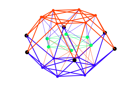
Figure 8: Ocneanu graph for $\mathcal{E}_{5}$

References

- [1] B. Bakalov, A. Kirillov Jr., Lectures on tensor categories and modular functors, AMS, Univ. Lect. Notes Series Vol.21(2001).
- [2] J. Böckenhauer and D. Evans; Modular invariants, graphs and induction for nets of subfactors II. Commun. Math. Phys. 200, 57-103 (1999).
- [3] J. Böckenhauer and D. Evans; Modular invariants from subfactors D. Evans lectures at Bariloche Summer School, Argentina, Jan 2000. AMS Contemporary Mathematics 294, R. Coquereaux, A. García and R. Trinchero eds.
- [4] P. Bouwknegt and K. Schoutens, W-symmetry in Conformal Field Theory Phys. Rep. 223 183-276 (1993).
- [5] P. Bouwknegt, J. McCarthy and K. Pilch, The W3 algebra: Modules, semi-infinite cohomology and BV-algebras, Lect. Notes in Physics: Monographs 42 (Springer Verlag, Berlin, 1996).
- [6] A. Cappelli, C. Itzykson and J.B.Zuber, Nucl. Phys. B 280 (1987) 445-465; Comm.Math. Phys. 113 (1987) 1-26.
- [7] A. Cappelli, C. Itzykson et J.-B. Zuber; The ADE classification of minimal and conformal invariant theories. Commu. Math. Phys. 13,1 (1987).
- [8] J.Cardy, Nucl.Phys. B 270 (1986) 186-204; J.Cardy, Nucl.Phys. B 275 (1986) 200-218, Nucl.Phys. B 324 (1989) 581-596.
- [9] R. Coquereaux, Notes on the quantum tetrahedron, Moscow Math. J. vol2, n1, Jan.-March 2002, 1-40, hep-th/0011006.
- [10] R. Coquereaux; Classical and quantum polyhedra: A fusion graph algebra point of view AIP Conference Proceedings 589 (2001), 37th Karpacz Winter School of Theor. Phys., J. Lukierski and J. Rembielinski eds, 181-203, hep-th/0105239.
- [11] R. Coquereaux, G. Schieber, Twisted partition functions for boundary conformal field theories and Ocneanu algebras of quantum symmetries, J. of Geom. and Phys. 781 (2002), 1-43, hep-th/0107001.
- [12] R. Coquereaux, G. Schieber, Determination of quantum symmetries for higher systems from the modular matrix, Jour. of Math. Phys. (to appear), hep-th/0203242.
- [13] R. Coquereaux, A. Garcia, G. Schieber, R. Trinchero, Ocneanu bi-algebras for diagrams and quantum groupoïds, to appear.
- [14] A. Coste and T. Gannon, Congruence subgroups and rational conformal field theory, math.QA/9909080.
- [15] P. Di Francesco and J.-B. Zuber, in Recent developments in Conformal Field Theory, Trieste Conference, 1989, S. Randjbar-Daemi, E. Sezgin and J.-B. Zuber eds, World Scientific, 1990; P. Di Francesco, Int. J. of Mod. Phys. A7, 92, 407.
- [16] P. Di Francesco and J.-B. Zuber; lattice integrable models associated with graphs, Nucl. Phys. B338, 602 (1990).
- [17] P. Di Francesco, P. Mathieu and S. Sénéchal; Conformal Field Theory, Springer 1997.
- [18] J.M. Drouffe, C. Itzykson, Theorie statistique des champs, Vol I et II, Savoirs Actuels, InterEditions, CNRS (1989).
- [19] D. Evans and Y. Kawahigashi, Quantum symmetries and operator algebras, Clarendon Press, 1998.
- [20] J. Fuchs, I. Runkel and C. Schweigert, TFT construction of RCFT correlators I: Partition functions, hep-th/0204148.
- [21] T. Gannon, The Classification of affine su(3) modular invariants, Comm. Math. Phys. 161, 233-263 (1994).
- [22] A. Hurwitz; Uber endliche Gruppen, welche in der Theorie der elliptschen Transzendenten auftreten Math. Annalen 27, 183-233 (1886).
- [23] F.M. Goodman, P. de la Harpe and V.F.R Jones, Coxeter graphs and towers of algebras, MSRI publications 14 (Springer, 1989).
- [24] Y. Kawahigashi and R. Longo, Classification of Local Conformal Nets. Case , math-ph/0201015.
- [25] A. Kirillov Jr and V. Ostrik, On q-analog of McKay correspondence and ADE classification of conformal field theories, math.QA/0101219.
- [26] J. McKay; Graphs, singularities and finite groups Proc. Symp. Pure Math. 37, 183 (1980).
- [27] A. Ocneanu; Quantized groups, string algebras and Galois theory for algebras. Warwick (1987), in Operator algebras and applications, Lond Math Soc Lectures note Series 136, CUP (1988).
- [28] A. Ocneanu; Paths on Coxeter diagrams: from Platonic solids and singularities to minimal models and subfactors. Talks given at the Centre de Physique Théorique, Luminy, Marseille, 1995.
- [29] A. Ocneanu; Paths on Coxeter diagrams: from Platonic solids and singularities to minimal models and subfactors. Notes taken by S. Goto, Fields Institute Monographs, AMS 1999, Rajarama Bhat et al, eds.
- [30] A. Ocneanu; Quantum symmetries for CFT-models A. Ocneanu, The Classification of subgroups of quantum SU(N), Lectures at Bariloche Summer School, Argentina, Jan.2000, AMS Contemporary Mathematics 294, R. Coquereaux, A. García and R. Trinchero eds.
-
[31]
A. Ocneanu, Higher Coxeter systems, Talk given
at MSRI,
http://www.msri.org/publications/ln/msri/2000/subfactors/ocneanu. - [32] V. Pasquier; Two-dimensional critical systems labelled by Dynkin diagrams Nucl.Phys. B285, 162 (1987).
- [33] P.A. Pearce and Yk Zhou; Intertwiners and A-D-E lattice models, IJMPhys B, Vol 7, Nos 20-21 (1993) 3469.
- [34] C.H.O. Chui, C. Mercat, W.P. Orrick and P. Pearce Integrable lattice realizations of conformal twisted boundary conditions Phys. Lett. B, 517:429-435, 2001.
- [35] C.H.O. Chui, C. Mercat and P. Pearce Integrable and conformal twisted boundary conditions for A-D-E lattice models hep-th/0210301.
- [36] J.-B. Zuber; Phys. Lett. B176, 127 (1986)
- [37] V.B.Petkova, J.-B.Zuber; Conformal Boundary conditions and what they teach us, hep-th 0103007, Generalized twisted partition functions, hep-th/0011021
- [38] V.B. Petkova and J.-B. Zuber; The many faces of Ocneanu cells, Nucl. Phys. B 603(2001) 449, hep-th/0101151
- [39] J.-B. Zuber; Graphs, algebras, conformal field theories and integrable lattice models, Nucl. Phys. B (Proc. Suppl.) 18B (1990) 313 - 326Generalized Dynkin diagrams and root systems and their folding, YITP International Workshop on Recent Developments in QCD and Hadron Physics, Kyoto, Japan, 16-18 Dec 1996, hep-th/9707046.
- [40] J.-B. Zuber; Lectures at Bariloche Summer School, Argentina, Jan 2000. AMS Contemporary Mathematics 294, R. Coquereaux, A. García and R. Trinchero eds. hep-th/0006151