Inflation and de Sitter Thermodynamics

Abstract

We consider the quasi-de Sitter geometry of the inflationary universe. We calculate the energy flux of the slowly rolling background scalar field through the quasi-de Sitter apparent horizon and set it equal to the change of the entropy (1/4 of the area) multiplied by the temperature, $dE=TdS$. Remarkably, this thermodynamic law reproduces the Friedmann equation for the rolling scalar field. The flux of the slowly rolling field through the horizon of the quasi-de Sitter geometry is similar to the accretion of a rolling scalar field onto a black hole, which we also analyze. Next we add inflaton fluctuations which generate scalar metric perturbations. Metric perturbations result in a variation of the area entropy. Again, the equation $dE=TdS$ with fluctuations reproduces the linearized Einstein equations. In this picture as long as the Einstein equations hold, holography does not put limits on the quantum field theory during inflation. Due to the accumulating metric perturbations, the horizon area during inflation randomly wiggles with dispersion increasing with time. We discuss this in connection with the stochastic decsription of inflation. We also address the issue of the instability of inflaton fluctuations in the “hot tin can” picture of de Sitter horizon.

I Introduction

The inflationary paradigm established during the last 20 years assumes that the primordial equation of state is almost vacuum-like: $p\approx-\epsilon$. To realize this equation of state, most models deal with a scalar field $\phi(t)$ (or other fields which in combination act as an effective scalar field) slowly rolling to the minimum of its potential $V(\phi)$. During the slow roll regime the homogeneous scalar field produces geometry which can be well approximated by the quasi-de Sitter metric.

The full pure de Sitter spacetime, which corresponds to a 4d hyperboloid of constant curvature, can be compactly represented by its Penrose diagram, given by the full square in Fig. 1. It can be covered by different coordinates. Cosmologists most often use coordinates in which the metric is time-dependent and corresponds to an expanding flat universe

$$ds^{2}=-dt^{2}+e^{2Ht}\left(dr^{2}+r^{2}d\Omega^{2}\right)\ ,$$ (1)

where $d\Omega^{2}=d\theta^{2}+\sin^{2}\theta d\phi^{2}$. This coordinate system covers the upper half of the hyperboloid, which corresponds to the expansion branch. The Penrose diagram of de Sitter spacetime in flat FRW coordinates is shown on the left panel of Fig. 1. Quasi-de Sitter geometry is described by the scale factor $a(t)=a_{0}\,e^{\int dtH(t)}$, where the Hubble parameter $H$ is a slowly varying function of time, $\dot{H}\ll H^{2}$.

                 

FIG. 1.: Penrose diagram of de Sitter spacetime in the flat FRW coordinates (left) and the static coordinates (right). Each point represent a sphere $S^{2}$. Its radius at the horizon (dashed line on the left, edge of diamond on the right) is equal to $\frac{1}{H}$.

The time-dependent form of the metric (1) is very convenient for investigating the dynamics of a scalar field with the equation

$$\Box\phi=V_{,\phi}$$ (2)

and for quantizing this field in the de Sitter spacetime [1]. Among quantum scalar fields with mass $m$ and conformal coupling $\xi$ in de Sitter geometry, the case of minimal coupling $\xi=0$ and very small mass $m\ll H$ plays an especially important role. Indeed, the regularized vacuum expectation value is $\langle\delta\phi^{2}\rangle=\frac{3H^{4}}{8\pi^{2}m^{2}}$. Formally, as was noted before the discovery of inflation, this is an odd case since its eigen-spectrum contains an infrared divergent term: $\langle\delta\phi^{2}\rangle\to\infty$ as $m\to 0$. On the other hand, this is the most interesting case for application to inflation, since the theory of inflaton (as well as tensor) fluctuations is reduced exactly to this case. Following the time evolution of individual fluctuations, it was found that the infrared divergence can be interpreted as the instability of quantum fluctuations of a very light scalar field, which are accumulated with time $\langle\delta\phi^{2}\rangle=\frac{H^{3}}{4\pi}\,t$ [2, 3, 4]. Fluctuations of $\delta\phi$ induce scalar metric perturbations [5, 4, 6, 7, 8]. This picture is a basis of the inflationary paradigm so successfully confirmed observationally. Notice that heavy or conformal fields are not produced by inflation. Further, backreaction of fluctuations $\delta\phi$ leads to the picture of stochastic evolution of quasi-de Sitter geometry [9, 10], and at large values of $H$ even to self-reproduction (eternal) of the inflationary universe [11]. Scalar field in the eternal inflationary universe is described naturally in terms of the probability distribution function $P(\phi,t)$ [10, 12].

Recently, de Sitter spacetime and inflation have drawn significant attention in the theoretical physics/superstring community. Some of the most interesting topics are holography and the thermodynamics associated with the de Sitter horizon. In this context, the static form of the metric of the de Sitter spacetime

$$ds^{2}=-(1-H^{2}\,R^{2})d\tau^{2}+{{dR^{2}}\over{(1-H^{2}\,R^{2})}}+R^{2}d\Omega^{2}\$$ (3)

is commonly used. The Penrose diagram of de Sitter spacetime in static coordinates is plotted on the right panel of Fig. 1. The classical result of [13] is that observer at the origin detects a thermal radiation from the de Sitter horizon at $R=\frac{1}{H}$ with the temperature $T=\frac{H}{2\pi}$, and the horizon area $A=\frac{4\pi}{H^{2}}$ is associated with the huge (geometrical) entropy $S=\frac{A}{4G}$. Thermal vacuum in the causal patch (“hot tin can”) corresponds to the Bunch-Davies vacuum of the metric (1) [14, 15] and gives a complementary picture of scalar field(s) fluctuations. It is not clear to us, however, how quantum fluctuations in the “hot tin can” picture correspond to the instability of quantum inflaton fluctuations $\delta\phi$ and generation of metric perturbations. We will return to this point at the end of the paper.

One of the issues in the holographic approach is the bookkeeping of entropy of de Sitter spacetime. The holography bound declares that the geometrical entropy of the horizon exceeds the entropy of quantum states (of fields and particles) within the volume surrounded by the horizon. It was recently claimed that counting the entropy of quantum fluctuations generated during inflation in the “hot tin can” and comparing it to the change of the apparent horizon entropy violates the holography bound unless an ultra-violet cutoff of order of $\sim 10^{16}$ GeV in the momenta of fluctuations is imposed [16].

While it is expected that the approaches based on the time-dependent form of the de Sitter metric with unstable fluctuations and the static form of the de Sitter metric with thermal flux should give us complementary insights, their languages are apparently different. This is partly due to the difference between quasi-de Sitter and pure de Sitter geometries, and partly because different questions are addressed. However, we have to understand how these two different approaches to (quasi-)de Sitter geometry with a scalar field are compatible with each other with respect to such important issues as the generation of fluctuations, entropy and global geometry.

In this paper we consider a particular question of how the apparent horizon area $A$, or the entropy $S=\frac{A}{4G}$, vary due to the slow roll of the background scalar field and the generation of scalar metric perturbations during inflation. A novel element here is that we combine the concepts of a dynamical, slowly rolling background field and the instability of its fluctuations, with the concept of geometrical, holographic entropy.

In Section II, we will calculate a variation of the geometrical entropy due to the energy flux through the apparent horizon area. We find that, remarkably, the thermodynamical relation $\delta E=TdS$ is equivalent to the Einstein equation for the rolling inflaton field. In a sense, our derivation of a correspondence between thermodynamics and the Einstein equations for inflation is a realization of such a correspondence found in an inspiring paper [17] for local accelerating observers. However, we introduce a technique to treat the apparent horizon of $R\times S^{2}$ topology which is different from the description [17] of a local Rindler horizon for an accelerating observer.

As we will see, a non-vanishing flux is generated by the kinetic term $\dot{\phi}^{2}$ of the slowly rolling inflaton field. It turns out that this problem is very similar to the problem of the interaction of a homogeneous rolling scalar field with a runaway potential $V(\phi)$ and a black hole. In Section III, we switch our attention from inflation to black holes. A rolling scalar field interacting with a black hole is a transparent illustration of the energy flow of a light scalar field through a horizon.

In Section IV, we return to inflation. On top of the rolling background inflaton, we consider inflaton fluctuations $\delta\phi$, which generate scalar metric perturbations $\Phi$. We study the energy flux through the horizon including inhomogeneous $\delta\phi$ fluctuations and corresponding variations in the area of the horizon, or entropy $dS$, which are sensitive to the scalar metric perturbations $\Phi$. In this case, the calculations are more involved than the calculations for the homogeneous time dependent background field in Section II. This happens because there is no exact Killing vector generating the horizon. However, for metric perturbations which preserve spherical symmetry we still can define $TdS$ and compare it with the energy flux through the horizon.

In Section V, we argue that the metric perturbations generated from inflaton quantum fluctuations can indeed be treated as (locally) spherically symmetric. We apply the general formalism for spherically symmetric non-static geometry of Section IV to fluctuations from inflation. Again, we find that the thermodynamical relation $\delta E=TdS$ leads to equations connecting $\Phi$ and $\delta\phi$ which are in exact agreement with the linearized Einstein equations for the fluctuations from inflation. This allows us to give new insights into the entropy of cosmological fluctuations, as we will discuss in Section VI.

II Slowly rolling inflaton and de Sitter entropy

We begin with an inflaton scalar field in the spacetime (1). The homogeneous background field $\phi(t)$ is time-dependent and obeys the equation (2), which for the metric (1) reads $\ddot{\phi}+3H\dot{\phi}+V_{,\phi}=0.$ If the Hubble parameter is large, the friction term here is significant and $\phi$ slowly rolls towards the minimum of $V(\phi)$, realizing the inflation.

The apparent horizon of de Sitter spacetime has the topology of $R^{1}\times S^{2}$, and is shown in Fig. 1 in both coordinate systems of interest. Imagine a spherical light front propagating from outside towards an observer at the origin $r=0$ or $R=0$. In the time-dependent coordinates the space is exponentially expanding. There is a critical, trapped surface $S^{2}$, which separates the region inside the apparent horizon which is in causal contact with the observer, and the outside region, where expansion keeps the light from reaching the inside region. The instant physical radius of an $S^{2}$ sphere is equal to $\rho=a(t)r$. Since the position of the apparent horizon is $r=\frac{1}{a(t)H}$, its radius $\rho_{\text{h}}$ is equal to $\frac{1}{H}$. It is constant in the pure de Sitter space time, and a slightly increasing function of time in the quasi-de Sitter geometry where $H(t)$ slowly decreases with time.

So far we have not used the Einstein equations, which relate the energy momentum tensor $T^{\mu}_{\nu}=\phi^{\mu}\phi_{\nu}-\left(\frac{1}{2}\phi^{\sigma}\phi_{\sigma}-V(\phi)\right)\delta^{\mu}_{\nu}$ of the background inflaton field $\phi(t)$ to the scale factor $a(t)$. Actually, we are going to derive them from the first law of thermodynamics of the de Sitter horizon.

Let us calculate the flux of energy through the area $A=\frac{4\pi}{H^{2}}$ of the apparent horizon of the quasi-de Sitter spacetime. In the spirit of the adiabatic approximation, we will treat the horizon as a static surface for this purpose, but allow it to slowly vary with time when calculating the change in its area. The energy flux through the horizon is given by the integral

$$\delta E=\delta\int d\Sigma_{\mu}\,T^{\mu}_{\nu}\,\xi^{\nu},$$ (4)

where $d\Sigma_{\mu}$ is the 3-volume of the horizon, and $\xi^{\mu}$ is the null generator of the horizon, as sketched in Fig. 5. Notice that at the horizon $d\Sigma^{\mu}$ is parallel to $\xi^{\mu}$, as both are null. We will equate the energy flux through the horizon to the change of geometrical entropy $dS$

$$TdS=\delta E=\delta\int d\Sigma_{\mu}\,T^{\mu}_{\nu}\,\xi^{\nu}\ ,$$ (5)

where the temperature $T$ is defined by the surface gravity at the horizon. For the de Sitter horizon, $T=\frac{H}{2\pi}$.

The entropy $dS$ and the expression (4) are geometrical invariants and can be calculated in arbitrary coordinates. In the case of de Sitter geometry we can work either in time-dependent (1) or static (3) coordinates. The metric (1) can easily be modified for the (adiabatic) regime of slowly rolling $H(t)$, while it is not so straightforward for the static form of the metric. Therefore, we will work in time-dependent coordinates. Consider a slowly rolling inflaton $\phi(t)$ that is time-dependent but homogeneous in the coordinates (1). The background stress-energy tensor $T^{\mu}_{\nu}$ is diagonal. As the (approximate) Killing vector is $\xi^{\mu}=(1,-Hr,0,0)$, the energy flux through the horizon $T_{\mu\nu}\,\xi^{\mu}\xi^{\nu}=\dot{\phi}^{2}$ is non-zero. To calculate the right hand side of equation (5), we integrate over the infinitesimal volume $4\pi\,\frac{1}{H^{2}}\,d\lambda$, where $\lambda$ is the affine parameter along the null generators of the apparent horizon. In the left hand side of (5), the variation of the entropy is $dS=\frac{dA}{4G}=-\frac{2\pi}{G}\,\frac{dH}{H^{3}}$. By comparing both sides of the thermodynamic equation (5) and dividing them by $d\lambda=dt$, we obtain

$$\dot{H}=-4\pi G\,\dot{\phi}^{2}\ .$$ (6)

This is nothing else but one of the Einstein equations. Using the equation of motion for $\phi$ and the equation (6), and assuming the field $\phi$ is dominant, one can reconstruct the Friedmann equation for $H$. Note that for a pure de Sitter geometry $\dot{\phi}=0$ and the energy flux through horizon is absent.

Formula (6) can also be derived from (5) in the coordinates (3). The coordinates $(t,r)$ of (1) and $(\tau,R)$ of (3) are related by the transformations

$$r=e^{H\tau}\,\frac{R}{\sqrt{1-H^{2}R^{2}}}\ ,\,\,\,\,\,\,t=\tau+\frac{1}{2H}\ln(1-H^{2}R^{2})\ .$$ (7)

In static coordinates, we have $\phi=\phi\left(\tau+\frac{1}{2H}\ln(1-H^{2}R^{2})\right)$. This $\phi(\tau,R)$ dependence corresponds to the field profile delayed as $R$ approaches the horizon. We find a similar delayed field configuration in black hole spacetimes in the next Section. The energy flux through the horizon $T^{\tau}_{R}=\phi_{,\tau}\phi_{,R}\sim\dot{\phi}^{2}$ is non-vanishing. In these coordinates, however, a central observer does not see the flux going through the horizon but rather accumulating the energy just outside the horizon. To quantify this, one can define the local mass function $M$ as it is done in Appendix B.

To conclude this section, we consider a sub-dominant, test scalar field $\chi$ during inflation. We can calculate the flux of the field $\chi$ through the de Sitter horizon. In this case, it is not important whether we are dealing with pure de Sitter or quasi-de Sitter geometry. Independent of the potential $V(\chi)$, the $\chi$-field contribution to the energy flux $\delta E$ is given by precisely the same expression as the inflaton field contribution. Either in terms of the thermodynamic equation $TdS=\delta E$ or in terms of the Einstein equations (6), the contribution of $\chi$ is additive

$$\dot{H}=-4\pi G\,(\dot{\phi}^{2}\ +\dot{\chi}^{2})\ .$$ (8)

This formula works even if the inflaton field velocity is sub-dominant, $\dot{\phi}\ll\dot{\chi}$, and independent of the shape of the $\chi$-field potential. In particular, it works for a massive scalar field $\chi$, which oscillates about the minimum with an exponentially decreasing amplitude.

III Rolling scalar field and Black Hole

In this section we interrupt the discussion of the slowly rolling inflaton in the early universe and focus on the seemingly different topic of a scalar field accreting into a black hole. The reader of the de Sitter story can jump to the next Section.

Consider a homogeneous scalar field $\phi(t)$ with a runaway type potential $V(\phi)$, say $V\sim 1/\phi^{2}$ or $V(\phi)\sim e^{-\phi/M_{P}}$. The concrete form of the potential is not important. We can even broaden the class of models to include fields with the potential $V(\phi)=\frac{1}{2}m^{2}\phi^{2}$ with very small masses $m$, as long as we deal only with the phase of slow roll towards the minimum. The well-known case of a massive scalar field oscillating around its minimum will have qualitatively different accretion onto a black hole similar to the accretion of massive (quasi)-particles.

We will consider a test homogeneous (cosmological) scalar field described by the equation (2). In the vicinity of a black hole, the spacetime is described by the Schwarzschild metric

$$ds^{2}=-\left(1-\frac{2M}{r}\right)dt^{2}+{{dr^{2}}\over{(1-\frac{2M}{r})}}+r^{2}d\Omega^{2}\ ,$$ (9)

and we will treat the cosmological evolution of the scalar field as the boundary conditions imposed sufficiently far away from the black hole. The scalar field retains its spherical symmetry $\phi=\phi(t,r)$, so near a black hole it obeys the equation (2)

$$\left[\frac{\partial^{2}\ }{\partial r_{*}^{2}}-\frac{\partial^{2}\ }{\partial t^{2}}-\left(1-\frac{2M}{r}\right)\,\frac{2M}{r^{3}}\right]\Big{(}r\phi(r,t)\Big{)}-\left(1-\frac{2M}{r}\right)\,V_{,\phi}=0,$$ (10)

where the tortoise coordinate $r_{*}$ is defined as $r_{*}=r+2M\ln(r/M-2)$. The field asymptotics at the horizon $r\to 2M$ corresponds to an infalling wave $\phi(t+r_{*})$. The boundary conditions far away from the black hole follow from the assumption that there the cosmological field is spatially uniform and is free to roll down the field potential. We take $\phi(t,r)=\phi_{\infty}(t)$ at $r\gg 2M$, where the time dependent function $\phi_{\infty}(t)$ is the background evolution of the field in the absence of the black hole. The function $\phi_{\infty}(t)$ depends on the scalar field potential $V(\phi)$.

Equation (10) is well studied for the case of a massive scalar field $V(\phi)=\frac{1}{2}m^{2}\phi^{2}$, where it can be reduced to a linear Schrödinger-type ordinary differential equation with an effective potential $U_{\text{eff}}(r)$.

However, in general the equation (10) is non-linear and the behavior of its solution is very different from the case of a massive scalar field; compare Figures 4 and 4. We treat equation (10) as a partial differential equation and solve it numerically for several examples of runaway potentials. We also consider the case of a very light massive field and compare it with the case of a heavy massive field.

The sequence of radial profiles $\phi(t,r)$ for several moments $t$ is shown in Figure 4 for a runaway potential and in Figure 4 for a very light massive field, respectively.

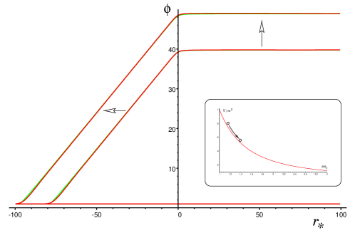
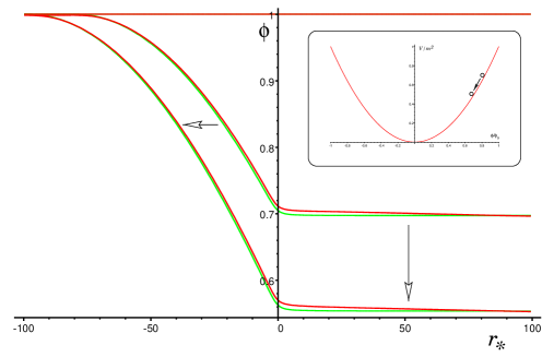
FIG. 2.: Field profiles $\phi(t,r)$ outside a black hole for the runaway potential $V(\phi)=1/\phi^{2}$ at two subsequent time moments; horizontal axis is a tortoise coordinate $r_{*}$. Red (solid) curves are the numerical solutions, and green (pale) curves are obtained with the delayed field approximation. The horizontal line corresponds to the homogeneous initial conditions.

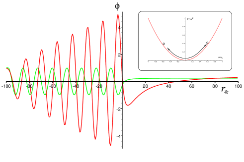
FIG. 3.: Field profiles for the potential $V(\phi)=\frac{1}{2}m^{2}\phi^{2}$ with a very small mass $m$ at two subsequent time moments. Red (solid) curves are the numerical solutions, and green (pale) curves are the delayed field approximations.

FIG. 4.: A snapshot of the field profile for the potential $V(\phi)=\frac{1}{2}m^{2}\phi^{2}$ with a large mass $m$ when the field oscillates. Red (solid) curve is the numerical solution, and green (pale) curve is the delayed field approximation.

We found that $\phi(t,r)$ in these cases with a very high accuracy can be approximated by a simple formula

$$\phi(t,r)=\phi_{\infty}\left[t+2M\ln\left(1-\frac{2M}{r}\right)\right]\ .$$ (11)

This result is rather insensitive to the form of the runaway potential. We will call the solution (11) the delayed field approximation. This is because the field profile is merely delayed, not frozen, on the horizon. In the Eddington-Finkelstein coordinates $(v,r)$ the incoming light geodesic is $v=t+r_{*}$. The solution (11) near the horizon is $\phi\approx\phi(v-v_{0})$ so the field crosses the horizon at the speed of light, but is delayed by a small amount $v_{0}=(2\ln 2-1)M$ compared to the null characteristic. Far away from the black hole, at large $r\gg 2M$, a long-range tail is formed, which can be described by the formula

$$\phi(t,r)\approx\phi_{\infty}(t)-\frac{(2M)^{2}}{r}\,\dot{\phi}_{\infty}(t)\ .$$ (12)

For a light massive field when the equation (10) is linear, the tail (12) can be related to scattering on the effective potential $U_{\text{eff}}(r)$ with a sharp peak at $\approx 3M$.

Our approximation (11), verified by the numerical solutions, generalizes the similar analytic result of [19] for the case of a free scalar field ($V=0$), where $\phi_{\infty}(t)=t$. The accuracy of the delayed field approximation can be estimated by substituting the expression (11) into the differential equation (10) and calculating the residual term which is of order ${\cal O}\left(\frac{2M}{r}(1-\frac{(2M)^{3}}{r^{3}})\right)$. The residual is bounded and localized at around $3M$; this is why the approximation (11) works.

Equipped with equation (11), we can calculate the energy flux of the scalar field through the horizon and the accretion rate onto the black hole $\dot{M}=\frac{dM}{dt}$. We can calculate $\dot{M}$ in different coordinates. In Schwarzschild coordinates, the spatial gradient of $\phi$ develops just outside the horizon, and the energy flux is defined by $T^{t}_{r}=\phi_{,t}\phi_{,r}\sim\dot{\phi}_{\infty}^{2}$. In these coordinates, an observer at asymptotic infinity does not actually see the energy flux go through the horizon. What she/he sees is the energy from accretion accumulating just outside the Schwarzschild radius, increasing the black hole mass (defined in the ADM sense). In the Eddington-Finkelstein coordinates, the energy flux through the horizon is given by $T_{vv}=\dot{\phi}_{\infty}^{2}$.

Independent of the choice of coordinates, the rate of accretion of the scalar field $\phi$ by a black hole and the rate of increase of its mass in the regime of the delayed field approximation is equal to

$$\dot{M}=4\pi(2GM)^{2}\,\dot{\phi}_{\infty}^{2}$$ (13)

It is easy to check that this formula is equivalent to the first law of black hole thermodynamics $\delta E=TdS$. We can rewrite (13) in the form $\left(\frac{1}{4GM}\right)^{.}=-4\pi G\,\dot{\phi}_{\infty}^{2}$, which is readily similar to the corresponding formula (6) for the slow roll scalar field in quasi-de Sitter geometry.

If we turn to the case of a massive scalar field with $V(\phi)=\frac{1}{2}m^{2}\phi^{2}$, when the background scalar oscillates around the minimum, we find that the delayed field approximation (11) quickly fails, see Figure 4, and formula (13) is not valid. In this case the scalar field can be described in the WKB approximation. The accretion of the massive scalar field looks like accretion of free massive quasi-particles of mass $m$. Notice that this is different from a massive oscillating scalar field in the de Sitter background, where the flux of the heavy scalar field through the horizon remains the same as for the light slow roll field, $\sim\dot{\phi}^{2}$.

In Appendix A, we briefly discuss some astrophysical applications of the results of this section.

IV Perturbed metric and horizon thermodynamics

Classical perturbations in the de Sitter geometry die out in accordance with the “no-hair” theorem. Therefore, as in the black hole case, there are well-defined concepts of the entropy $S$ and temperature $T$ associated with the pure de Sitter horizon [13].

The spherical symmetry of the spacetime naturally selects a foliation by surfaces of the constant physical radius $\rho=\text{const}$, with normal vector $\nabla_{\mu}\rho$. If the spacetime is static (i.e admits a timelike Killing vector field $k^{\mu}$ with vanishing differential invariant $k_{\mu;\nu}k_{\beta}\varepsilon^{\mu\nu\beta\alpha}$; do not mix with static form of the metric), as de Sitter spacetime is for example, the vector $\xi^{\mu}=-\varepsilon^{\mu\nu}\nabla_{\nu}\rho$ orthogonal to $\nabla_{\mu}\rho$ is also a Killing vector and a null generator of the event horizon (which coincides with the apparent and Killing horizons in the static case). Therefore one can define the surface gravity at the horizon $\kappa$ by $\xi^{\nu}\xi_{\mu;\nu}=\kappa\xi_{\mu}$ and identify $\kappa=H$ and the temperature in the usual way $T=\frac{H}{2\pi}$. The area entropy is equal to $1/4$ of the apparent horizon area in the Planck units, $S=\frac{\pi}{GH^{2}}$.

For the quasi-de Sitter geometry with the homogeneous scalar field $\phi(t)$ slowly rolling towards its minimum, when the horizon radius $1/H(t)$ is adiabatically changing with time, we still can introduce an entropy $S=\frac{\pi}{G}\,\frac{1}{H(t)^{2}}$ and temperature $T=\frac{H(t)}{2\pi}$ associated with the apparent horizon.

In inflationary cosmology, classical perturbations which could exist prior to inflation die out. However, one of the striking features of the quasi-de Sitter inflationary stage is that the quantum fluctuations of the light (minimally coupled to gravity) scalar field $\delta\phi$ are unstable and inevitably generate scalar metric perturbations $\Phi(t,\vec{x})$ [5, 21], so that the quasi-de Sitter metric (1) becomes perturbed

$$ds^{2}=-(1+2\Phi)dt^{2}+(1-2\Phi)e^{2\int dtH}\left(dr^{2}+r^{2}d\Omega^{2}\right)\ .$$ (14)

If the spacetime is not static (timelike Killing vector does not exist), as in the inflationary geometry (14), the situation with the horizon thermodynamics is not quite so simple. The event horizon and apparent horizon are in general different surfaces, and the Killing horizon does not exist, so the notion of surface gravity is ill-defined.

Fortunately, in the case of spherical symmetry one can define the mass (energy) $M$ inside the spherical region of the physical radius $\rho$ by $1-\frac{2GM}{\rho}=(\nabla\rho)^{2}$. The mass function $M$ obeys the mass formula [18] which follows from the Einstein equations

$$M_{;a}=4\pi\rho^{2}(T_{ab}-Tg_{ab})\rho^{;b},$$ (15)

where $a,b$ stands for $(t,r)$ only. We derive the mass formula (15) in Appendix B and give there other definitions to be used in this Section.

We will argue now that the mass formula (15) applied at the apparent horizon can be interpreted as a first law of thermodynamics $\delta E=TdS$ for an arbitrary spherically symmetric metric. In the next section, we will apply this result to the perturbed inflationary metric (14), which as we will show can be well treated as (locally) spherically symmetric.

Let us look at the apparent horizon, as it is locally defined and much easier to find than an event horizon. In spherical symmetry, the position of the apparent horizon is given by $f\equiv(\nabla\rho)^{2}=0$. The vector $\nabla_{a}f$ is normal to the apparent horizon, which is the surface $f=0$, while the orthogonal vector $\zeta^{a}=\varepsilon^{ab}\nabla_{b}f$ is tangent to it. Unlike in the static case, these vectors are not necessary null. The change of the mass function $M$ along the apparent horizon is trivially related to the change of the radius of apparent horizon,

$$G\zeta^{a}M_{;a}=\kappa\rho\zeta^{a}\rho_{;a}=\frac{\kappa}{2\pi}\,\zeta^{a}(\pi\rho^{2})_{;a}\ ,$$ (16)

which allows its interpretation as the first law of thermodynamics

$$\stackrel{{\scriptstyle\delta E}}{{\overbrace{\zeta^{a}M_{;a}}}}\ =\ \stackrel{{\scriptstyle T}}{{\overbrace{\frac{\kappa}{2\pi}}}}\ \stackrel{{\scriptstyle dS}}{{\overbrace{\zeta^{a}\left(\frac{A}{4G}\right)_{;a}}}}\ .$$ (17)

The parameter $\kappa$ is defined in the Appendix B and generalizes the surface gravity. To relate the heat flow term with the stress-energy tensor, we use the mass formula (15) which gives

$$\zeta^{a}M_{;a}=4\pi\rho^{2}(T_{a}^{b}-Tg_{a}^{b})\zeta^{a}\rho_{;b}.$$ (18)

The above expression can be rewritten in a more convenient form if one realizes that $\zeta^{a}M_{;a}=-2\kappa\xi^{a}M_{;a}$

$$-\zeta^{a}\left(\frac{A}{8\pi G}\right)_{;a}=2{A}\,T_{a}^{b}\xi^{a}\rho_{;b}.$$ (19)

This formula relates the change of the apparent horizon area to the (spherically symmetric) flux of matter through the $\rho=\text{const}$ surface passing through the point on the horizon at which $M$ is evaluated.

V Fluctuations from inflation and wiggles of the horizon area

In the time-dependent metric (1) of the quasi-de Sitter geometry, quantum fluctuations of the inflaton scalar field can be expanded with respect to the eigenmodes

$$\hat{\delta}\phi(t,\vec{x})=\sum_{lm}\int dk\,\left(\hat{a}_{klm}\,\phi_{klm}+\hat{a}_{klm}^{+}\,\phi_{klm}^{*}\right)\ ,$$ (20)

where $\hat{a}_{klm}$ and $\hat{a}^{+}_{klm}$ are annihilation and creation operators; $\phi_{klm}=\phi_{k}(t)\,2kj_{l}(kr)\,Y_{lm}(\vec{\Omega})$ are the eigenmodes. The $r-$dependent eigenmode factor is given in terms of the spherical Bessel functions $j_{l}(kr)$, $Y_{lm}(\vec{\Omega})$ are the spherical harmonics, and the time-dependent eigenmode factor is given in terms of Hankel functions $\phi_{k}(t)=\frac{\sqrt{\pi}}{2}\,H\eta^{3/2}\,{\cal H}^{(1)}(k\eta)$, where $\eta$ is the conformal time $\eta=-\frac{1}{H}e^{-Ht}$. The Bunch-Davies vacuum corresponds to the absence of particles in the past $\hat{a}_{klm}|0\rangle=0.$ This corresponds to the positive-frequency asymptotic $\phi_{k}(t)\simeq\frac{1}{\sqrt{2k}}e^{-ik\eta}$ in the far past $\eta\to-\infty$. Quantum fluctuations of the inflaton field are unstable and turn into long-wavelength classical inhomogeneities. Indeed, the modes which have physical wavelengths smaller than the horizon $1/H$, have $k\eta\gg 1$ at the horizon and quickly oscillate without producing physical effects. In contrast, the modes with the wavelengths which exceed the horizon size $k\eta=k\leq 1$ cease to oscillate, freeze out, and look like a classical scalar field with amplitude $\phi_{k}(t)\approx\frac{H}{\sqrt{2}k^{3/2}}$.

We need to know the form of the eigenmodes at the apparent horizon where $r=\eta$. Again, the time-oscillating modes with small physical wavelengths $kr=k\eta\gg 1$ are spatially oscillating functions $j_{l}(kr)$. Large wavelengths modes with $kr=k\eta\ll 1$ have asymptotics $j_{l}(kr)\sim(kr)^{l}$. Notably, only the $s$-wave with $l=0$ survives in this asymptotic. Therefore, in our discussion of the wiggles of the horizon area due to metric fluctuations, we can consider only spherically symmetric perturbations.

Fluctuations $\delta\phi$ generate scalar metric perturbations which are represented in (14) by scalar $\Phi(t,r)$. Now we are going to relate $\delta\phi$ and $\Phi$ using the apparent horizon thermodynamics.

In the perturbed spacetime (14), the physical radius is $\rho=(1-\Phi)\,e^{\int dtH}\,r$. Apparent horizon is defined by $(\nabla\rho)^{2}=0$. From here we find for the apparent horizon

$$\rho_{\text{h}}=H^{-1}\left(1+\Phi+\frac{\dot{\Phi}}{H}-\frac{\Phi_{,r}}{\dot{a}}\right).$$ (21)

The entropy of the apparent horizon and the temperature are identified with geometrical quantities as

$$S=\frac{A}{4G}=\frac{\pi\rho_{\text{h}}^{2}}{G},\hskip 20.00003ptT=\frac{\kappa}{2\pi}=\frac{1}{4\pi\rho_{\text{h}}},$$ (22)

where $\kappa$ is defined by equation (34) of Appendix B. Evaluating the equation (19) relating the change in the horizon area to the energy flux at the position of the apparent horizon in the perturbed spacetime (14), and keeping only the linear terms with respect to $\Phi$, $\delta\phi$, and their derivatives, one finds the following expression for the perturbations

$$\ddot{\Phi}-\frac{2}{a}\,\dot{\Phi}_{,r}+\frac{1}{a^{2}}\,\Phi_{,rr}+H\dot{\Phi}=8\pi G\,\dot{\varphi}\left(\delta\dot{\varphi}-\frac{1}{a}\,\delta\varphi_{,r}\right),$$ (23)

valid at the position of the apparent horizon.

Even though we know already that the first law of thermodynamics (17) originated from the Einstein equations in the form of (15), and hence the above equation would follow from the linearized Einstein equations, let us explicitly demonstrate this fact. The usual equations for metric perturbations from scalar field fluctuations are [21]

$$\left(1+\frac{\nabla^{2}_{\vec{x}}}{4\pi G\,a^{2}\dot{\varphi}^{2}}\right)\Phi=\left(\frac{\delta\varphi}{\dot{\varphi}}\right)^{.}\ ,\hskip 20.00003pt\frac{(a\Phi)^{\dot{}}}{a}=4\pi G\,\dot{\varphi}\delta\varphi\ ,$$ (24)

where the for spherically symmetric $\Phi$, $\nabla^{2}_{\vec{x}}\Phi=\partial_{rr}\Phi+\frac{2}{r}\partial_{r}\Phi$. Combining both equations by substituting them into an identity $2\dot{\varphi}\delta\dot{\varphi}=\dot{\varphi}^{2}\left(\frac{\delta\varphi}{\dot{\varphi}}\right)^{.}+(\dot{\varphi}\delta\varphi)^{\dot{}},$ we find that

$$\ddot{\Phi}-\frac{2}{a}\,\dot{\Phi}_{,r}+\frac{1}{a^{2}}\,\Phi_{,rr}+H\dot{\Phi}+\frac{2}{a^{2}}\left(\frac{1}{r}-\dot{a}\right)\Phi_{,r}=8\pi G\,\dot{\varphi}\left(\delta\dot{\varphi}-\frac{1}{a}\,\delta\varphi_{,r}\right)\ .$$ (25)

This equation holds everywhere in the perturbed spacetime. When evaluated at the apparent horizon, the last term in the left-hand side vanishes and we are left exactly with the equation (23).

Consider the area of the apparent horizon $A=4\pi\rho_{h}^{2}$. For frozen long-wavelength fluctuations, we can drop derivatives in formula (21) for $\rho_{\text{h}}$. Then the leading contribution of the frozen classical fluctuations to area is

$$A=\frac{4\pi}{H^{2}}\,\left(1+2\Phi\right)\ .$$ (26)

Thus, the quantum fluctuations of the inflaton field generate wiggles of the quasi-de Sitter horizon area, as described by (26) and sketched in Figure 5.

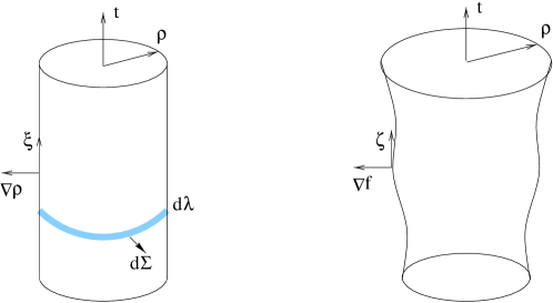
FIG. 5.: A sketch of the apparent horizon of radius $\rho$. Left: the horizon in quasi-de Sitter geometry where $\rho=\frac{1}{H}$ very slowly increases with time. Right: the same but with small metric perturbations where $\rho=\frac{1}{H}(1+\Phi)$ is wiggling with time due to the randomly varying $\Phi$.

Locally (within the Hubble patch), almost spherical metric perturbation $\Phi$ can be viewed as the variation of the Hubble parameter $H$ [4, 12]. Indeed, transform the metric (14) to synchronous coordinates $\tilde{t}=t+\int^{t}dt\Phi$, $\tilde{x}_{i}=x_{i}+\int^{t}\frac{dt}{a}\int\nabla_{i}\Phi$. Then we have $ds^{2}=-d\tilde{t}^{2}+e^{2\int d\tilde{t}\tilde{H}}d\tilde{x}^{2}$, where the new Hubble parameter is $\tilde{H}=(1-\Phi)H$. As expected, the area of the horizon is the same

$$A=\frac{4\pi}{H^{2}}\,\left(1+2\Phi\right)=\frac{4\pi}{\tilde{H}^{2}}\ .$$ (27)

Therefore an observer within a Hubble patch sees the local Hubble parameter $\tilde{H}$ simultaneously slow rolling and wiggling due to the instability of quantum fluctuations of the inflaton field, in the spirit of stochastic picture of inflation.

We have to note that there is another, much smaller correction to the geometrical entropy due to the back reaction of quantum field effects in curved background. Indeed, quantum gravity effects give one-loop corrections of order of $R^{2}\sim H^{4}$ in the right hand side of the Einstein equations, which slightly shift the Hubble parameter [22] and the horizon area by a factor $1+c\frac{H^{2}}{M_{p}^{2}}$, where $c$ is some numerical coefficient. However, this leads to a tiny correction in the area entropy.

Let us discuss the formula (26). Metric fluctuations $\Phi(t,r)\sim\delta\phi$ have a flat spectrum $\Phi_{k}=C\,\frac{V^{3/2}}{M_{p}^{3}V_{,\phi}}\,\frac{1}{k^{3/2}}$, where $C=\frac{16}{15}(3\pi)^{3/2}$ is a numerical coefficient. Classical fluctuations of the inflaton field $\delta\phi$ can be treated as a random (Wiener) process with zero vacuum expectation value, but with the increasing dispersion $\langle\delta\phi^{2}\rangle\sim\int^{aH}\frac{dk}{k}=\frac{H^{3}}{4\pi^{2}}t$. Suppose for a moment that the background value of $H(t)$ is changing very slowly. Then, scalar metric fluctuations $\Phi(t,r)$ have zero mean value but their dispersion is increasing with time linearly, $\langle\Phi^{2}\rangle=C^{2}\,\frac{V^{3}}{M_{p}^{6}V_{,\phi}^{2}}\int^{aH}\frac{dk}{k}\sim t$. Thus, the area of the apparent horizon looks like a random (Wiener) process with the mean value $\bar{A}=\frac{4\pi}{H(t)^{2}}$ and with the dispersion $\langle\Phi^{2}\rangle$ linearly increasing with time. Imagine an ensemble of inflationary Hubble patches with apparent horizon areas given by the formula (26). Then their area is a statistical value which obeys the Gaussian distribution $P(A,t)\sim e^{-\frac{(A-\bar{A})^{2}}{2\langle\Phi^{2}\rangle}}$. Now, if we take into account variation of background values like $H(t)$ and $V(\phi(t))$ with time, time-dependence and statistical properties of the horiazon area given by (26) or equivalently (27) will be more complicated. We will discuss this issue below.

VI Discussion: Entropy and Cosmological Fluctuations

In this paper we calculated the apparent horizon area and geometrical entropy of quasi-de Sitter geometry, which describes an inflationary stage, and the energy flux of the scalar fields through the apparent horizon. Issues related to de Sitter thermodynamics are commonly considered in the static de Sitter coordinates, where an observer at the origin is surrounded by the event horizon and detects a thermal flux of temperature $T=\frac{H}{2\pi}$.

We work with the geometrical entropy $S$ of the apparent horizon in the time-dependent planar de-Sitter coordinates adopted in inflationary cosmology, which admit a simple generalization to the quasi-de Sitter geometry and, most importantly, admit a clear interpretation of fluctuations generated from inflation.

The slow roll of the inflaton field leads to slow change in the horizon radius. Assuming that the energy flux of the rolling scalar field through the horizon changes the geometrical entropy $\delta E=TdS$, we reproduce the Einstein equation (6) which relates $\dot{H}$ and $\dot{\phi}^{2}$. Other background scalars $\chi$ which are subdominant during inflation give similar contributions to the energy flux $\dot{\chi}^{2}$, independent of their potentials.

This change of the quasi-de Sitter horizon radius due to the rolling scalar field is very similar to the increase of the mass of a black hole due to the accretion of a background scalar field rolling towards the minimum of its potential $\dot{M}\sim\dot{\phi}^{2}$. This type of accretion, which can be described analytically with the delayed field approximation, can be realized for runaway potentials of the background scalar field or for very light massive fields. We present this material here mainly to illustrate similar calculations for rolling scalars in quasi-de Sitter geometry, as the astrophysical effects of accretion of a rolling scalar onto a black hole that we considered (say quintessence and astrophysical-size black holes) are negligibly small. Oscillating heavy scalar field accretes onto black hole very differently as quasi-particles.

Inflationary, quasi-de Sitter stage erases classical inhomogeneities which could exist prior to it. However, quantum fluctuations of the inflaton field (as well as other light scalars minimally coupled to gravity) are unstable and produce long-wavelength fluctuations of the inflaton field $\delta\phi$ which behave as classical inhomogeneities at scales larger than the Hubble patch of size $H^{-1}$. Fluctuations $\delta\phi$ generate long-wavelength scalar metric perturbations $\Phi$. Geometrical quantities, like an area of the apparent horizon, acquire corrections due to the scalar metric perturbations. We calculate the energy flux of the inhomogeneous scalar field $\phi(t)+\delta\phi(t,\vec{x})$ through the apparent horizon and the change in the apparent horizon area of the perturbed metric multiplied by its (geometrical) temperature $TdS$. Again, equating $\delta E=TdS$, we show that this thermodynamics relation is compatible with the linearized Einstein equations which relate $\Phi$ and $\delta\phi$.

Thus, as long as the Einstein equations hold, generation of the inflaton fluctuations is in full agreement with the variation of the entropy of the quasi-de Sitter horizon. Therefore, in the picture of rolling inflaton with quantum fluctuations generated with time, we did not find that quantum fluctuations may violate holographic bound during inflation. (Notice that the fluctuations from inflation are described by squeezed states, which do not carry entropy [23, 24]. In simple terms, locally the effect of fluctuations is just a wiggling of the local Hubble parameter).

It was suggested in [16] that in the “hot tin can” picture the entropy of fluctuations may violate holographic bound during inflation. The issue of inflaton fluctuations in the “hot tin can” picture is not clear to us. In theory of inflation, scalar field fluctuations are usually considered in the time dependent metric (1), as it was described in Section V. Bunch-Davies vacuum corresponds to the thermal state in the static coordinates. On the other hand, in the static de Sitter coordinates, discussion of the quantum field theory is usually restricted to thermal radiation from the horizon, usually in terms of the detector response. Thermal radiation associated with the de Sitter horizon is related to any free quantum field, scalar fields with mass $m$ and any coupling to gravity, vector fields etc., the difference will be only in the radial dependence of the wave functions (“gray-body factor”). On the other hand, instability of quantum fluctuations from inflation occurs only for very light minimally coupled scalar fields. It will be interesting to understand what is relation of the quantum field theory in the “hot tin can” picture, and the instability of fluctuations from inflation. For this it will be essential to work with regularized VEV $<\delta\phi^{2}>$.

As we already mentioned, in the picture of rolling scalar field with accumulating inflaton fluctuations, which we adopt in the paper, holographic bound and quantum fluctuations from inflation are compatible.

A lesson from our calculations is that in the quasi-de Sitter geometry with slowly rolling scalar field, the horizon area, or geometrical entropy, are perturbed by the scalar metric fluctuations according to the formulas (26), (27). This means that the area of the horizon for an ensemble of the different Hubble patches is not the same but is a statistical variable by itself. For small metric perturbations (of order of $\Phi\sim\frac{H}{M_{p}}$), its mean value is $\bar{A}=\frac{4\pi}{H^{2}}$, where $H(t)$ is slowly decreasing background value, but dispersion around the mean value is defined by $\langle\Phi^{2}\rangle$, which growth with time. Equivalently, we can talk about statistical properties of the local Hubble values $\tilde{H}$ [4, 12]. Notably, this picture is converging with the stochastic description of inflation in terms of the probability distribution of the inflaton field [9, 10, 12]. Probability to have the value of inflaton field $\phi$ in quasi-static regime is $P(\phi)\sim\exp{\left(-\frac{3M_{p}^{4}}{8V(\phi)}\right)}$ and can be interpreted in terms of entropy $S=\log P(\phi)$ [25]. Remarkably, this entropy is identical to the geometrical entropy $\frac{A}{4G}$. During inflation and rolling of $\phi$ the Wiener process of accumulating fluctuations $\delta\phi$ (or similarly perturbations of $\Phi$) changes distribution of $P(\phi)$. Distribution of the horizon areas of different Hubble patches, defined by the local values of the Hubble parameters, depends on the background slow roll regime and the regime of accumulation of fluctuations, both of which depend on the model of inflation [9, 10, 12]. It would be interesting to understand further the correspondence between stochastic approach to inflation and geometrical entropy (26), (27).

So far we discussed small metric fluctuations $\Phi$ or small local variations of $H$. However, in the chaotic inflationary scenario for large enough values of $\phi$, variations of $H$ due to the quantum jumps of $\delta\phi$ can be large and lead to the self-reproducing inflationary universe [11]. We would like to draw attention to this regime (which is still below the Planck energy density) and to note that “adiabatic” geometrical thermodynamics which we considered in this paper is not applicable here. Indeed, consider the Hubble patch where $H$ is increasing due to the quantum jumps. Increase of $H$ is not compatible with the classical Einstein equation (6). Consequently, quantum jumps are not compatible with the horizon thermodynamics (of a single Hubble patch) since $\delta E=TdS$ does not hold either. Geometrical entropy of the local Hubble patch is decreasing. However, we have to take into account the entropy of all Hubble patches. Self-reproduction of inflating regions looks like a chain reaction, which is described by the branching diffusion process [26].

Appendix A: Rolling Cosmic Scalars and Black Holes

Here we briefly discuss astrophysical applications of the results of Section III. One of the most important examples of slowly rolling scalar field is a homogeneous cosmological scalar field, whose evolution is given by the field equation $\ddot{\phi}+3H\dot{\phi}+V_{,\phi}=0$ with the Hubble friction. This type of fields appears, for instance, in the cosmological models of quintessence. To dominate at the present cosmological stage while avoiding gravitational clustering, the value of $\phi$ should be of order of the Planck mass $M_{P}$, and its effective mass $m^{2}_{\text{eff}}=V_{,\phi\phi}$ very small, $m^{2}_{\text{eff}}\leq H$, where $H(t)$ in the present day Hubble parameter.

Quintessence may interact gravitationally with black holes of different masses, ranging from tiny primordial black holes to astrophysical black holes of solar masses to supermassive black holes. Accretion of quintessence onto a black hole is given by the formula (13). Scalar field velocity $\dot{\phi}(t)_{\infty}$ is defined by its equation of motion; however, the kinetic energy $\dot{\phi}^{2}$ cannot exceed the total energy density of the universe $M_{P}^{2}H^{2}$. Substituting this upper limit in (13), we estimate the rate of the black hole growth due to the accretion of the rolling cosmological scalar field

$$\dot{M}\sim H^{2}M^{2}\sim\left(\frac{r_{g}}{H^{-1}}\right)^{2}\ ,$$ (28)

where $r_{g}=2M$ is the gravitational radius of the black hole, $H^{-1}$ is the size of the universe, and we switched to Planck units $M_{P}=1$. Thus, accretion of cosmic scalars including quintessence is absolutely negligible for all types of astrophysical black holes. For primordial black holes at the moment of formation, when the ratio $\left(\frac{r_{g}}{H^{-1}}\right)$ is of order of unity, the study of Section III of rolling scalar field accretion is not applicable directly, as the black hole spacetime would be significantly different from Schwarzschild in this case. Even if one believes the equation (13) in this regime, it would seem unlikely that the accretion of quintessence can cause explosive growth of primordial black holes (contrary to some claims in the literature). For this to occur, the seed primordial black hole would have to be much bigger than the cosmological horizon if the quintessence is subdominant.

It is interesting to take into account the back reaction of an accretion on the evolution of the cosmic scalar field itself. From the energy balance we obtain a correction to the Hubble friction term due to the accretion of rolling scalar onto black holes

$$\ddot{\phi}+(3H+n_{\text{BH}}r_{g}^{2})\dot{\phi}+V^{\prime}(\phi)=0\ ,$$ (29)

where $n_{\text{BH}}$ is the spatial density of black holes. This correction is proportional to the filling factor of black holes, i.e. the fraction of volume occupied by black holes. The last is tiny so that the effect of the interaction of a rolling scalar field with black holes is negligible.

Rolling scalar field interacting with a black hole also emerges in the context of the Brans-Dicke or more general scalar-tensor theories [20, 19].

Appendix B: Mass Formula in Spherical Symmetry

A general spherical spacetime is described by the metric

$$ds^{2}=g_{ab}\,dx^{a}dx^{b}+\rho^{2}d\Omega^{2},$$ (30)

where $g_{ab}$ is the metric on a two-manifold with coordinates $(t,r)$, and $\rho$ is the physical radius of spherical slices. The field dynamics is given by the Einstein-Hilbert action, which in spherical symmetry can be dimensionally reduced to yield

$$S=\int\sqrt{-\gamma}\,d^{2}x\,\left\{{\textstyle\frac{1}{16\pi G}}\left[\rho^{2}R[\gamma]+2(\nabla\rho)^{2}+2\right]+\rho^{2}{\cal L}_{\text{matter}}\right\}.$$ (31)

The Einstein equations for spherically symmetric spacetime (30) follow from the above action by varying it with respect to the two-metric $g_{ab}$ and the two-scalar $\rho$. In particular, the $\{ab\}$ component of the Einstein equations is

$$2\rho^{-1}[g_{ab}\Box\rho-\rho_{;ab}]+\rho^{-2}g_{ab}[(\nabla\rho)^{2}-1]=8\pi G\,T_{ab}.$$ (32)

By subtracting the (two-dimensional) trace, this equation can be written in a more convenient form

$$\rho_{;ab}-\kappa g_{ab}=-4\pi G\,\rho(T_{ab}-Tg_{ab}),$$ (33)

where we have defined

$$\kappa=\frac{1}{2\rho}[1-(\nabla\rho)^{2}]\ .$$ (34)

In the case of Schwarzschild black hole, $\kappa$ coincides with the surface gravity at the horizon. We will continue to use the same notation since $\kappa$ defined in (34) will enter the thermodynamics relation in the more general case.

In spherical symmetry, it is possible to define a local mass function $M(x^{a})$ by

$$1-\frac{2GM}{\rho}=(\nabla\rho)^{2}\equiv f$$ (35)

The change in mass is related to the flux of matter given by the stress-energy tensor $T_{ab}$. To see this, let us take the derivative of $M=\frac{\rho}{2}\,(1-f)$

$$GM_{;a}=-\frac{\rho}{2}(f_{;a}-2\kappa\rho_{;a})=-\rho(\rho_{;ab}-\kappa g_{ab})\rho^{;b}$$ (36)

and use the Einstein equation (33) we derived above to obtain

$$M_{;a}=4\pi\rho^{2}(T_{ab}-Tg_{ab})\rho^{;b}.$$ (37)

This is the differential mass formula in a spherically symmetric spacetime [18].

REFERENCES

- [1] T. S. Bunch and P. C. Davies, Quantum field theory in de Sitter space: Renormalization by point splitting, Proc. Roy. Soc. Lond. A 360, 117 (1978).
- [2] A. Vilenkin and L. H. Ford, Gravitational effects upon cosmological phase transitions, Phys. Rev. D 26, 1231 (1982);
- [3] A. D. Linde, Scalar field fluctuations in expanding universe and the new inflationary universe scenario, Phys. Lett. B 116, 335 (1982);
- [4] A. A. Starobinsky, Dynamics of phase transition in the new inflationary universe scenario and generation of perturbations, Phys. Lett. B 117, 175 (1982).
- [5] V. F. Mukhanov and G. V. Chibisov, Quantum fluctuation and ’nonsingular’ universe, JETP Lett. 33, 532 (1981);
- [6] S. W. Hawking, The development of irregularities in a single bubble inflationary universe, Phys. Lett. B 115, 295 (1982).
- [7] A. H. Guth and S. Y. Pi, Fluctuations in the new inflationary universe, Phys. Rev. Lett. 49, 1110 (1982).
- [8] J. M. Bardeen, P. J. Steinhardt and M. S. Turner, Spontaneous creation of almost scale-free density perturbations in an inflationary universe, Phys. Rev. D 28, 679 (1983).
- [9] A. Vilenkin, The birth of inflationary universes, Phys. Rev. D 27, 2848 (1983).
- [10] A. A. Starobinsky, Stochastic de Sitter (inflationary) stage in the early universe, in Current trends in field theory, quantum gravity and strings, Eds. H. de Vega and N. Sanches, Lect. Notes in Phys. Springer-Verlag 246 107 (1986).
- [11] A. D. Linde, Eternally existing selfreproducing chaotic inflationary universe, Phys. Lett. B 175, 395 (1986).
- [12] A. S. Goncharov, A. D. Linde and V. F. Mukhanov, The global structure of the inflationary universe, Int. J. Mod. Phys. A 2, 561 (1987).
- [13] G. W. Gibbons and S. W. Hawking, Cosmological event horizons, thermodynamics, and particle creation, Phys. Rev. D 15, 2738 (1977).
- [14] R. Bousso, A. Maloney and A. Strominger, Conformal vacua and entropy in de Sitter space, Phys. Rev. D 65, 104039 (2002) [hep-th/0112218].
- [15] N. Kaloper, M. Kleban, A. Lawrence, S. Shenker and L. Susskind, Initial conditions for inflation, JHEP 0211, 037 (2002) [hep-th/0209231].
- [16] A. Albrecht, N. Kaloper and Y. S. Song, Holographic limitations of the effective field theory of inflation, hep-th/0211221.
- [17] T. Jacobson, Thermodynamics of space-time: The Einstein equation of state, Phys. Rev. Lett. 75, 1260 (1995) [gr-qc/9504004].
- [18] E. Poisson and W. Israel, Internal structure of black holes, Phys. Rev. D 41, 1796 (1990).
- [19] T. Jacobson, Primordial black hole evolution in tensor scalar cosmology, Phys. Rev. Lett. 83, 2699 (1999) [astro-ph/9905303].
- [20] J. D. Barrow and B. J. Carr, Formation and evaporation of primordial black holes in scalar - tensor gravity theories, Phys. Rev. D 54, 3920 (1996).
- [21] V. F. Mukhanov, Gravitational instability of the universe filled with a scalar field, JETP Lett. 41, 493 (1985).
- [22] L. A. Kofman, A. D. Linde and A. A. Starobinsky, Inflationary universe generated by the combined action of a scalar field and gravitational vacuum polarization, Phys. Lett. B 157, 361 (1985).
- [23] R. H. Brandenberger, T. Prokopec and V. Mukhanov, The entropy of the gravitational field, Phys. Rev. D 48, 2443 (1993) [gr-qc/9208009].
- [24] C. Kiefer, D. Polarski and A. A. Starobinsky, Entropy of gravitons produced in the early universe, Phys. Rev. D 62, 043518 (2000) [gr-qc/9910065].
- [25] A. D. Linde, Quantum creation of an open inflationary universe, Phys. Rev. D 58, 083514 (1998) [gr-qc/9802038].
- [26] A. Linde, D. Linde and A. Mezhlumian, From the Big Bang theory to the theory of a stationary universe, Phys. Rev. D 49, 1783 (1994) [arXiv:gr-qc/9306035].