Abstract

Classical geometry of de Sitter spacetime is reviewed in arbitrary dimensions. Topics include coordinate systems, geodesic motions, and Penrose diagrams with detailed calculations.

1 Introduction

Cosmological constant $\Lambda$ was originally introduced in general relativity with the motivation to allow static homogeneous universe to Einstein equations in the presence of matter. Once expansion of the universe was discovered, its role turned out to be unnecessary and it experienced a checkered history. Recent cosmological observations suggest some evidences for the existence of a positive cosmological constant [1] : From a variety of observational sources, its magnitude is $(G\hbar/c^{3})\Lambda\sim 10^{-123}$, and both matter $\Omega_{\rm matter}$ and vacuum $\Omega_{\Lambda}$ are of comparable magnitude, $\Omega_{\rm matter}/\Omega_{\Lambda}\sim 0.3/0.7$ in spatially flat universe. Both results are paraphrased as old and new cosmological constant problems [2, 3]. Inclusion of quantum field theory predicts naturally the energy density via quantum fluctuations even up to the Planck scale, so the old problem is to understand why the observed present cosmological constant is so small. It is the worst fine-tuning problem requiring a magic cancellation with accuracy to 120 decimal places. The new problem is to understand why the vacuum energy density is comparable to the present mass density of the universe. Though there are several classes of efforts to solve the cosmological constant problem, e.g., cancellation of vacuum energy based on symmetry principle like supersymmetry, the idea of quintessence, and the anthropic principle, any of them is not widely accepted as the solution, yet. In the early universe, existing cosmological constant also provides an intriguing idea, inflationary cosmology, to fix long-standing cosmological problems in the Big-bang scenario.

In addition to the above, detailed properties of the de Sitter geometry in arbitrary dimensions raise a debate like selection of true vacuum compatible with its scale symmetry in relation with trans-Planckian cosmology [4, 5] or becomes a cornerstone of a theoretical idea like dS/CFT for a challenging problem of quantum gravity in de Sitter spacetime [6].

In the context of general relativity, classical study on the cosmological constant is to understand geometry of de Sitter spacetime (dS_d). Therefore, in this review, we study de Sitter geometry and the motion of classical test particle in the background of the de Sitter spacetime in detail. Topics include useful coordinate systems, geodesic motions, and Penrose diagrams. One of our purposes is to combine knowledges of classical de Sitter geometry, scattered with other subjects in the textbooks or reviews, in one note [7, 8, 9, 10]. We tried to make our review self-contained and a technical note by containing various formulas in the appendix.

The review is organized as follows. In section 2, we introduce our setup with notations and signature. In section 3, four coordinates (global, conformal, planar, and static) and coordinate transformations among those are explained with the reason why such four of them are frequently used. Killing symmetries are also obtained in each coordinate system. All possible geodesic motions of classical test particle are given in section 4. Identification of de Sitter horizon for a static observer and cosmological evolution to a comoving observer are also included. In section 5, causal structure of the global de Sitter spacetime is dealt through Penrose diagrams, and its quantum theoretical implication is also discussed. Section 6 is devoted to brief discussion. Various quantities are displayed in Appendix for convenience.

2 Setup

In this section, we introduce basic setup for studying classical geometry of de Sitter spacetime in arbitrary dimensions. Two methods are employed : One is solving directly Einstein equations for each metric ansatz, and the other is reading off the specific form of coordinate transformation between two metrics.

We begin with Einstein-Hilbert action coupled to matters :

$$S=\frac{1}{16\pi G}\int d^{d}x\,\sqrt{-g}\,(R-2\Lambda)+S_{\rm m},$$ (2.1)

where $S_{\rm m}$ stands for the matter action of our interest, which vanishes for limit of the pure gravity, and $\Lambda$ is a cosmological constant, which sets to be positive for dS_d. Einstein equations are read from the action (2.1)

$$G_{\mu\nu}+\Lambda g_{\mu\nu}=8\pi GT_{\mu\nu},$$ (2.2)

where energy-momentum tensor $T_{\mu\nu}$ is defined by

$$T_{\mu\nu}\equiv-\frac{2}{\sqrt{-g}}\frac{\delta{S}_{\rm m}}{\delta g^{\mu\nu}}.$$ (2.3)

Throughout the paper small Greek indices $\mu,\nu,\rho,\sigma,\tau,\kappa...$ run from $0$ to $d-1$, and our spacetime signature is $(-,+,+,\dots,+)$.

To be specific let us consider a real scalar field $\phi(x)$ of which action is

$$S_{\rm m}=\int d^{d}x\sqrt{-g}\left[-\frac{1}{2}g^{\mu\nu}\partial_{\mu}\phi\partial_{\nu}\phi-V(\phi)\right].$$ (2.4)

In order not to have an additional contribution to the cosmological constant at classical level, we set minimum value of the scalar potential to vanish, ${\rm min}(V(\phi))=0$. Then its energy-momentum tensor becomes

$$T_{\mu\nu}=\partial_{\mu}\phi\partial_{\nu}\phi-\frac{1}{2}g_{\mu\nu}\partial_{\rho}\phi\partial^{\rho}\phi-g_{\mu\nu}V(\phi),$$ (2.5)

where energy density $T_{00}$ is positive semi-definite in the limit of flat spacetime.

For the pure dS_d, the energy-momentum tensor of the matter, $T_{\mu\nu}$, vanishes so that one can regard these spacetimes as solutions of the Einstein equations of Eq. (2.2)

$$G_{\mu\nu}=-\Lambda g_{\mu\nu}$$ (2.6)

for an empty spacetime with a positive constant vacuum energy $(\Lambda>0)$ :

$$T_{\mu\nu}^{\rm vacuum}\equiv\frac{\Lambda}{8\pi G}g_{\mu\nu}.$$ (2.7)

Therefore, the only nontrivial component of the Einstein equations (2.6) is

$$R=\frac{2d}{d-2}\Lambda>0.$$ (2.8)

It means that the de Sitter spacetime is maximally symmetric, of which local structure is characterized by a positive constant curvature scalar alone such as

$$R_{\mu\nu\rho\sigma}=\frac{1}{d(d-1)}(g_{\mu\rho}g_{\nu\sigma}-g_{\mu\sigma}g_{\nu\rho})R.$$ (2.9)

Since the scalar curvature (2.8) is constant everywhere, the dS_d is free from physical singularity and it is confirmed by a constant Kretschmann scalar :

$$R_{\mu\nu\rho\sigma}R^{\mu\nu\rho\sigma}=\frac{2}{d(d-1)}R^{2}=\frac{8d^{2}}{d(d-1)(d-2)^{2}}\Lambda^{2}.$$ (2.10)

We follow usual definition of tensors as follows.

quantity	definition
Jacobian factor	$g\equiv\det(g_{\mu\nu})$
connection	$\Gamma^{\mu}_{\nu\rho}\equiv\frac{1}{2}g^{\mu\sigma}(\partial_{\nu}g_{\sigma\rho}+\partial_{\rho}g_{\sigma\nu}-\partial_{\sigma}g_{\nu\rho})$
covariant derivative of a contravariant vector	$\nabla_{\mu}A^{\nu}\equiv\partial_{\mu}A^{\nu}+\Gamma^{\nu}_{\mu\rho}A^{\rho}$
Riemann curvature tensor	$R^{\mu}_{\;\;\nu\rho\sigma}\equiv\partial_{\rho}\Gamma^{\mu}_{\sigma\nu}-\partial_{\sigma}\Gamma^{\mu}_{\rho\nu}+\Gamma^{\mu}_{\rho\tau}\Gamma^{\tau}_{\sigma\nu}-\Gamma^{\mu}_{\sigma\tau}\Gamma^{\tau}_{\rho\nu}$
Ricci tensor	$R_{\mu\nu}\equiv R^{\rho}_{\;\mu\rho\nu}$
curvature scalar	$R\equiv g^{\mu\nu}R_{\mu\nu}$
Einstein tensor	$\displaystyle{G_{\mu\nu}\equiv R_{\mu\nu}-\frac{g_{\mu\nu}}{2}R}$

3 Useful Coordinates

When we deal with specific physics in general relativity, we are firstly concerned with appropriate coordinate system. In this section, we introduce four useful coordinates and build coordinate transformations among those for tensor calculus : They are global (closed), conformal, planar (inflationary), and static coordinates. For the detailed calculation of various quantities in systems of coordinates, refer to Appendix.

Similar to physical issues in flat spacetime, the symmetries of a Riemannian manifold is realized through metric invariance under the symmetry transformations. Specifically, let us choose a coordinate system as $(x^{\mu},g_{\mu\nu})$ and take into account a transformation $x^{\mu}\rightarrow x^{\prime\mu}$. If the metric $g_{\mu\nu}$ remains to be form-invariant under the transformation

$$g_{\mu\nu}^{\prime}(x)=g_{\mu\nu}(x)$$ (3.1)

for all coordinates $x^{\mu}$, such transformation is called an isometry. Since any finite continuous transformation with non-zero Jacobian can be constructed by an infinite sum of infinitesimal transformations, study under infinitesimal transformation is sufficient for continuous isometry. If we consider an infinitesimal coordinate transformation

$$x^{\mu}\rightarrow x^{\prime\mu}=x^{\mu}+\varepsilon X^{\mu}(x),$$ (3.2)

where $\varepsilon$ is small parameter and $X^{\mu}$ a vector field, expansion of the form-invariance (3.1) leads to Killing’s equations

$$L_{X}g_{\mu\nu}\equiv X^{\rho}\partial_{\rho}g_{\mu\nu}+g_{\mu\rho}\partial_{\nu}X^{\rho}+g_{\rho\nu}\partial_{\mu}X^{\rho}=0,$$ (3.3)

where $L_{X}$ denotes a Lie derivative. Then, any $X^{\mu}$ given by a solution of the Killing’s equations (3.3) is called a Killing vector field. In every subsection we will discuss Killing symmetries of each coordinate system.

3.1 Global (closed) coordinates $(\tau,\theta_{i}),~{}i=1,2,\cdots,d-1$

An intriguing observation about the dS_d is embedding of the dS_d into flat $(d+1)$-dimensional spacetime, which was made by E. Schrödinger (1956). In $(d+1)$-dimensional Minkowski spacetime, the Einstein equation is trivially satisfied

$$0 = {}^{d+1}R\equiv g^{AB}R_{AB}$$ (3.4)

$$= R+R_{dd},$$

where capital indices, $A,B,...$, represent $(d+1)$-dimensional Minkowski indices run from $0$ to $d$. If we set $R_{dd}=-\frac{2d}{d-2}\Lambda$ which implies a positive constant curvature of the embedded space, then the $d$-dimensional Einstein equation (2.8) of dS_d is reproduced.

Topology of such embedded $d$-dimensional spacetime of the positive constant curvature is visualized by urging algebraic constraint of a hyperboloid

$$\eta_{AB}X^{A}X^{B}=l^{2},$$ (3.5)

where $\eta_{AB}={\rm diag}(-1,1,1,\cdot\cdot\cdot,1)$. So the globally defined metric of flat $(d+1)$-dimensional spacetime is

$$ds^{2}=\eta_{AB}dX^{A}dX^{B}$$ (3.6)

constrained by the equation of a hyperboloid (3.5). Let us clarify the relation between the cosmological constant $\Lambda$ and the length $l$ by inserting the constraint (3.5) into the Einstein equation (2.8). To be specific, we eliminate the last spatial coordinate $X^{d}$ from the metric (3.6) and the constraint (3.5) :

$$dX^{d}=\mp\frac{\eta_{\mu\nu}X^{\mu}dX^{\nu}}{\sqrt{l^{2}-\eta_{\alpha\beta}X^{\alpha}X^{\beta}}}.$$ (3.7)

Inserting Eq. (3.7) into the metric (3.6), we have the induced metric $g_{\mu\nu}$ of a curved spacetime due to an embedding :

$$g_{\mu\nu}=\eta_{\mu\nu}+\frac{X_{\mu}X_{\nu}}{l^{2}-\eta_{\alpha\beta}X^{\alpha}X^{\beta}},$$ (3.8)

and its inverse $g^{\mu\nu}$ is

$$g^{\mu\nu}=\eta^{\mu\nu}-\frac{1}{l^{2}}X^{\mu}X^{\nu}.$$ (3.9)

The induced connection $\Gamma^{\mu}_{\nu\rho}$ becomes

$$\Gamma^{\mu}_{\nu\rho}=\frac{1}{l^{2}}\left(\eta_{\nu\rho}X^{\mu}+\frac{X_{\nu}X_{\rho}X^{\mu}}{l^{2}-\eta_{\alpha\beta}X^{\alpha}X^{\beta}}\right).$$ (3.10)

Subsequently, we compute induced curvatures : The Riemann curvature tensor $R^{\mu}_{\;\nu\rho\sigma}$ is

$$R^{\mu}_{\;\nu\rho\sigma}=\frac{1}{l^{2}}\left[\eta_{\nu\sigma}\delta{{}^{\mu}}{{}_{\rho}}-\eta_{\nu\rho}\delta{{}^{\mu}}{{}_{\sigma}}+\frac{\eta_{\nu\rho}X_{\sigma}X^{\mu}-\eta_{\nu\sigma}X_{\rho}X^{\mu}+\delta{{}^{\mu}}{{}_{\rho}}X_{\nu}X_{\sigma}-\delta{{}^{\mu}}{{}_{\sigma}}X_{\nu}X_{\rho}}{l^{2}-\eta_{\alpha\beta}X^{\alpha}X^{\beta}}\right]$$

$$+\frac{1}{l^{4}}\left[\eta_{\nu\sigma}X_{\rho}X^{\mu}-\eta_{\nu\rho}X_{\sigma}X^{\mu}+\frac{\left(\eta_{\nu\sigma}X_{\rho}X^{\mu}-\eta_{\nu\rho}X_{\sigma}X^{\mu}\right)X_{\gamma}X^{\gamma}}{l^{2}-\eta_{\alpha\beta}X^{\alpha}X^{\beta}}\right],~{}~{}~{}~{}~{}~{}~{}~{}~{}$$ (3.11)

and the Ricci tensor $R_{\mu\nu}$ is

$$R_{\mu\nu}=\frac{d-1}{l^{2}}\left(\eta_{\mu\nu}+\frac{X_{\mu}X_{\nu}}{l^{2}-\eta_{\alpha\beta}X^{\alpha}X^{\beta}}\right)\;.$$ (3.12)

Since the induced curvature scalar $R$ does not vanish

$$R=\frac{d(d-1)}{l^{2}},$$ (3.13)

the Einstein equation, (3.4) or (3.5), will determine the relation between the length $l$ and the cosmological constant $\Lambda$. Insertion of the constraint (3.5) into the Einstein equation (2.8) gives us a relation between the cosmological constant $\Lambda$ and the length $l$ such as

$$\Lambda=\frac{(d-1)(d-2)}{2l^{2}}.$$ (3.14)

Implemented by Weyl symmetry, the unique scale of the theory of our interest, $l$, can always be set to be one by a Weyl rescaling as

$$X^{A}\longrightarrow X^{{}^{\prime}{A}}=e^{-\omega}X^{A}=\frac{X^{A}}{l}.$$ (3.15)

Therefore, the dS_d is defined as a $d$-dimensional hypersurface (a hyperboloid) embedded in flat $(d+1)$-dimensional spacetime, and the overall topology is cylindrical, being $R\times S^{d-1}$ (See Fig. 1).

Figure 1: $d$-dimensional hyperboloid illustrating de Sitter spacetime embedded in $d+1$-dimensions.

A well-known coordinate system to cover entire $d$-dimensional hyperboloid is obtained from the following observation : As shown in Fig. 1, the relation between $X^{0}$ and the spatial length of $(X^{1},X^{2},...,X^{d})$ is hyperbolic and spatial sections of a constant $X^{0}$ defines a $(d-1)$-dimensional sphere of radius $\sqrt{l^{2}+(X^{0})^{2}}$. Therefore, a convenient choice satisfying Eq. (3.5) is

$$X^{0}=l\sinh\frac{\tau}{l}~{}~{}{\rm and}~{}~{}X^{\alpha}=l\omega^{\alpha}\cosh\frac{\tau}{l},~{}~{}(\alpha=1,...,d),$$ (3.16)

where $-\infty<\tau<\infty$ and $\omega^{\alpha}$’s$~{}(\alpha,\beta,...)$ for the spatial sections of constant $\tau$ satisfy

$$\sum_{\alpha=1}^{d}(\omega^{\alpha})^{2}=1.$$ (3.17)

Subsequently, we have $d-1$ angle variables $\theta_{i},~{}i=1,2,\cdots,d-1$, such as

$$\omega^{1} = \cos\theta_{1},\hskip 156.49014pt0\leq\theta{{}_{1}}<\pi,$$

$$\omega^{2} = \sin\theta_{1}\cos\theta_{2},\hskip 128.0374pt0\leq\theta{{}_{2}}<\pi,$$

$$\vdots$$

$$\omega^{d-2} = \sin\theta_{1}\cos\theta_{2}\cdots\sin\theta_{d-3}\cos\theta_{d-3},~{}\hskip 28.45274pt0\leq\theta_{d-3}<\pi,$$

$$\omega^{d-1} = \sin\theta_{1}\cos\theta_{2}\cdot\cdot\cdot\cdots\sin\theta_{d-2}\cos\theta_{d-1},\hskip 14.22636pt0\leq\theta_{d-2}<\pi,$$

$$\omega^{d} = \sin\theta_{1}\cos\theta_{2},\cdots\cdots\sin\theta_{d-2}\sin\theta_{d-1},\hskip 14.22636pt0\leq\theta_{d-1}<2\pi.$$ (3.18)

Inserting Eq. (3.16) and Eq. (3.1) into the metric (3.6), we have a resultant metric rewritten in terms of the above coordinates $(\tau,\theta_{i})$ :

$$ds^{2}=-d\tau^{2}+l^{2}\cosh^{2}\left(\frac{\tau}{l}\right)\,d\Omega^{2}_{d-1},$$ (3.19)

where $d\Omega^{2}_{d-1}$ is $(d-1)$-dimensional solid angle

$$d\Omega^{2}_{d-1} = d\theta_{1}^{2}+\sin^{2}\theta_{1}d\theta_{2}^{2}+\cdot\cdot\cdot+\sin^{2}\theta_{1}\cdot\cdot\cdot\sin^{2}\theta_{d-2}d\theta^{2}_{d-1}$$ (3.20)

$$= \sum_{j=1}^{d-1}\left(\prod_{i=1}^{j-1}\sin^{2}\theta_{i}\right)d\theta_{j}^{2}.$$

Note that singularities in the metric (3.20) at $\theta_{i}=0$ and $\theta_{i}=\pi\;(i=1,2,\cdots,d-2)$ are simply trivial coordinate artifacts that occur with polar coordinates. In these coordinates with a fixed time $\tau$, the spatial hypersurface corresponds to a $(d-1)$-dimensional sphere of radius $l\cosh(\tau/l)$. Thus, its radius is infinitely large at $\tau=-\infty$, decreases to the minimum radius $l$ at $\tau=0$, and then increases to infinite size as $\tau\rightarrow\infty$. We again emphasize that the spatial section is compact (finite) except for the farthest past and future. In this coordinate system, $\partial/\partial\theta_{d-1}$ is the only Killing vector because the metric (3.19) is isometric under the rotation of a coordinate $\theta_{d-1}$. On the other hand, $\partial/\partial\tau$ is not a Killing vector and missing of this Killing symmetry breaks the conservation of energy so that Hamiltonian is not defined properly and the quantization procedure does not proceed smoothly. However, $S$-matrix of the quantum field theory, if it exists, is known to be unitary because the coordinates cover globally the whole spacetime.

An opposite direction is to assume an appropriate form of metric with an unknown function $f(\tau/l)$,

$$ds^{2}=-d\tau^{2}+l^{2}f(\tau/l)^{2}d\Omega^{2}_{d-1},$$ (3.21)

and then to try to solve the Einstein equations. Curvature scalar of the metric (3.21) is computed as

$$R=(d-1)\frac{(d-2)(1+\dot{f}^{2})+2f\ddot{f}}{l^{2}f^{2}},$$ (3.22)

where the overdot denotes derivative of the rescaled time variable $\dot{f}\equiv df/d(\tau/l)$ in this subsection. With the aid of Eq. (3.14), the Einstein equation (2.8) becomes

$$2(f\ddot{f}-\dot{f}^{2}-1)=d(-\dot{f}^{2}+f^{2}-1).$$ (3.23)

A particular solution of Eq. (3.23), irrespective of $d$, can be obtained by solving two equations

$$f\ddot{f}-\dot{f}^{2}-1=0~{}~{}\mbox{and}~{}~{}-\dot{f}^{2}+f^{2}-1=0.$$ (3.24)

The solution of Eq. (3.24) is $\pm\cosh[(\tau-\tau_{0})/l]$ except unwanted trivial solution ($f=0$). Since we can choose $\tau_{0}=0$ without loss of generality, via a time translation, $\tau\rightarrow\tau-\tau_{0}$, we have

$$f(\tau/l)=\pm\cosh\left(\frac{\tau}{l}\right)$$ (3.25)

which is equivalent to the metric (3.19) found by a coordinate transformation. The general solution of Eq. (3.23) should satisfy the following equations

$$f\ddot{f}-\dot{f}^{2}-1=d{\cal F}~{}~{}\mbox{and}~{}~{}-\dot{f}^{2}+f^{2}-1=2{\cal F},$$ (3.26)

where ${\cal F}$ is an arbitrary function of $\tau/l$. According to the search by use of Mathematica and a handbook [11], it seems that no other solution than Eq. (3.25) is known, yet.

3.2 Conformal coordinates $(T,\theta_{i})$

A noteworthy property of the dS_d is provided by computation of the Weyl (or conformal) tensor

$$C_{\mu\nu\rho\sigma} = R_{\mu\nu\rho\sigma}+\frac{1}{d-2}(g_{\mu\sigma}R_{\rho\nu}+g_{\nu\rho}R_{\sigma\mu}-g_{\mu\rho}R_{\rho\nu}-g_{\nu\sigma}R_{\rho\nu})$$ (3.27)

$$+\frac{1}{(d-1)(d-2)}(g_{\mu\rho}g_{\rho\nu}-g_{\mu\sigma}g_{\sigma\nu})R,$$

for $d\geq 4$, or the Cotton tensor

$$C^{\mu\nu}=\frac{\epsilon^{\rho\sigma\mu}}{\sqrt{-g}}\nabla_{\sigma}\left(R{{}^{\nu}}{{}_{\rho}}-\frac{\delta^{\nu}_{\;\rho}}{4}R\right)$$ (3.28)

for $d=3$. Substituting the Einstein equation (2.8) and Eq. (2.9) into the conformal tensors in Eqs. (3.27) and (3.28), we easily notice that they vanish so that dS_d is proven to be conformally flat :

$$C_{\mu\nu\rho\sigma} = \left[\frac{1}{d(d-1)}-\frac{2}{d(d-2)}+\frac{1}{(d-1)(d-2)}\right](g_{\mu\rho}g_{\rho\nu}-g_{\mu\sigma}g_{\rho\nu})R=0,$$ (3.30)

$$C^{\mu\nu} = -\frac{1}{4}\frac{\epsilon^{\mu\nu\rho}}{\sqrt{-g}}\nabla_{\rho}(R-4\Lambda)\stackrel{{\scriptstyle R\sim\Lambda}}{{=}}0.$$ (3.31)

Therefore, the condition (2.9) that the Riemann curvature tensor is determined by the scalar curvature alone is equivalent to the condition of vanishing conformal tensor in this system. Consequently the unique scale of the dS_d, $l=\sqrt{(d-1)(d-2)/2\Lambda}$, can be scaled away by a Weyl (scale) transformation.

The above conformal property of the dS_d suggests that conformal coordinate system is a good coordinate system. It is written in terms of conformal time $T$ as

$$ds^{2}=F(T/l)^{2}(-dT^{2}+l^{2}d\Omega^{2}_{d-1}).$$ (3.32)

If we compare the metric of the global coordinates (3.19) with that of the conformal coordinates (3.32), then coordinate transformation between two is summarized in a first-order differential equation of $F(T/l)$

$$\frac{d\ln F}{dT}=\pm\sqrt{F^{2}-1}\;,$$ (3.33)

where $F(T/l)=\cosh(\tau/l)\geq 1$ provides a boundary condition such as $F(0)=1$. The unique solution of Eq. (3.33) is

$$F(T/l)=\sec\left(\frac{T}{l}\right).$$ (3.34)

Substituting the result (3.34) into the metric (3.32), we have

$$ds^{2}=\frac{1}{\cos^{2}\frac{T}{l}}(-dT^{2}+l^{2}d\Omega_{d-1}^{2})~{}\mbox{with}~{}-\frac{\pi}{2}<\frac{T}{l}<\frac{\pi}{2}.$$ (3.35)

Since the metric (3.35) is isometric under the rotation of $\theta_{d-1}$, $\partial/\partial\theta_{d-1}$ is a Killing vector but there is no other Killing vector. Thus, the only symmetry is axial symmetry. Note that there is one-to-one correspondence between the global coordinates (3.19) and the conformal coordinates (3.35), which means that the conformal coordinate system describes also entire de Sitter spacetime. In addition, any null geodesic with respect to the conformal metric (3.35) is also null in the conformally-transformed metric :

$$d\tilde{s}^{2}\equiv\cos^{2}\left(\frac{T}{l}\right)ds^{2}=-dT^{2}+l^{2}d\Omega_{d-1}^{2}.$$ (3.36)

Therefore, Penrose diagram for the dS_d can easily be identified from this metric (3.36), which contains the whole information about the causal structure of the dS_d but distances are highly distorted. However, we will discuss the Penrose diagram for the dS_d in section 5 after the Kruskal coordinate system is introduced. As mentioned previously, topology of the de Sitter spacetime is cylindrical $(R\times S^{d-1})$ so the process to make the Penrose diagram is to change the hyperboloid into a $d$-dimensional cylinder of a finite height, being $I\times S^{d-1}$ $(I=[0,\pi])$. Again note that the conformal coordinate system (3.35) does not include the timelike Killing symmetry so that the Hamiltonian as a conserved quantity cannot be chosen and the quantum theory on these coordinates is also sick. Existence of conformal symmetry also affects much on the choice of field theoretic vacuum in the de Sitter spacetime.

From now on let us obtain the conformal metric (3.34) by solving the Einstein equations (2.6) under Eq. (3.32). If we compute the curvature scalar, we have

$$R=(d-1)\frac{(d-2)F^{2}+(d-4)\dot{F}^{2}+2F\ddot{F}}{l^{2}F^{4}},$$ (3.37)

Here overdot denotes $\dot{F}\equiv dF/d(T/l)$, and the same overdot in every subsection will also be used as derivative of the rescaled time variable in each corresponding subsection. Then the Einstein equation (2.8) becomes

$$2(F\ddot{F}-F^{2}-2\dot{F}^{2})=d(F^{4}-\dot{F}^{2}-F^{2}).$$ (3.38)

A particular solution of Eq. (3.38), irrespective of $d$, should satisfy the following equations

$$F\ddot{F}-2\dot{F}^{2}-F^{2}=0~{}~{}\mbox{and}~{}~{}\dot{F}^{2}+F^{2}-F^{4}=0.$$ (3.39)

The unique solution of Eq. (3.39) with $F(0)=1$ is proven to be the same as Eq. (3.34). The general solution should satisfy the following equations

$$F\ddot{F}-F^{2}-2\dot{F}^{2}=d{\cal G}~{}~{}\mbox{and}~{}~{}F^{4}-\dot{F}^{2}-F^{2}=2{\cal G},$$ (3.40)

where ${\cal G}$ is an arbitrary function of $T/l$. According to the search by use of Mathematica and a handbook [11], no other solution than Eq. (3.34) is found yet.

3.3 Planar (inflationary) coordinates $({\sf t},x^{i})$

A noticed character of the pure dS_d from Eq. (2.9) is the fact that it is maximally symmetric. Suppose a comoving observer in the pure dS_d, then he or she may find maximally-symmetric spatial hypersurface orthogonal to his or her time direction. The corresponding planar (inflationary) metric takes the form

$$ds^{2}=-d{\sf t}^{2}+a^{2}({\sf t}/l)\gamma_{ij}dx^{i}dx^{j}\;,$$ (3.41)

where $a({\sf t}/l)$ is cosmic scale factor and $(d-1)$-dimensional spatial metric $\gamma_{ij}$ of hypersurface should also carry maximal symmetries as a defining property :

$${}^{d-1}R_{ijkl}=k(\gamma_{ik}\gamma_{jl}-\gamma_{il}\gamma_{jk})\;,$$ (3.42)

where $\displaystyle{k=\frac{a^{4}}{(d-1)(d-2)}\;{}^{d-1}R}$.

Note that every nonvanishing component of the $d$-dimensional Riemann curvature $R_{\mu\nu\rho\sigma}$ is expressed by the $(d-1)$-dimensional metric (3.41) such as

$$R_{{\sf t}i{\sf t}j} = -l^{2}a\ddot{a}\gamma_{ij}\;,$$ (3.43)

$$R_{{\sf t}ijk} = -a\dot{a}\left(\partial_{i}\gamma_{kj}+\partial_{j}\gamma_{ki}-\partial_{k}\gamma_{ij}\right)\;,$$ (3.44)

$$R_{ijkl} = (ka^{2}+a^{2}\dot{a}^{2})(\gamma_{ik}\gamma_{jl}-\gamma_{il}\gamma_{jk})\;,$$ (3.45)

where the overdot denotes derivative of the rescaled time variable, $\dot{a}\equiv da({\sf t}/l)/d({\sf t}/l)$. So does those of the Ricci tensor

$$R_{{\sf t}{\sf t}} = -\frac{d-1}{a}\ddot{a}\;,$$ (3.46)

$$R_{{\sf t}i} = \frac{\dot{a}}{a}\gamma^{jk}(\partial_{j}\gamma_{ik}-\partial_{i}\gamma_{jk}+\partial_{k}\gamma_{ji})\;,$$ (3.47)

$$R_{ij} = [a\ddot{a}+(d-2)(\dot{a}^{2}+k)]\gamma_{ij}\;,$$ (3.48)

and that of the scalar curvature

$${R=(d-1)\frac{2a\ddot{a}+(d-2)\dot{a}^{2}+(d-2)k}{a^{2}}}.$$ (3.49)

In the de Sitter spacetime of our interest, we only have a positive vacuum energy (or equivalently a positive cosmological constant) as the matter source given in Eq. (2.7). Let us interpret it in terms of a cosmological perfect fluid of which energy-momentum tensor can be written

$$T_{\mu\nu}=(p+\rho)U_{\mu}U_{\nu}+pg_{\mu\nu},$$ (3.50)

where $\rho$ and $p$ are the energy density and pressure respectively as measured in the rest frame, and $U_{\mu}$ is the velocity of the fluid. Since the fluid is at rest for a comoving observer, the velocity of the fluid $U_{\mu}$ is

$$U^{\mu}=(1,0,0,...,0),$$ (3.51)

and then $T^{\mu}_{\;\nu}\equiv{\rm diag}(-\rho,p,\dots,p)$. Therefore, the equation of state $w=p/\rho=-1$ tells it is a perfect fluid with a positive constant density and a negative constant pressure :

$$\rho=-p=\frac{\Lambda}{8\pi G}.$$ (3.52)

Obviously it is also consistent with conservation of the energy-momentum tensor (2.7), i.e., $\nabla_{\mu}T^{\mu}_{\;\nu}=0$.

Due to isotropy and homogeneity, spatial part of the metric (3.41) $\gamma_{ij}$ is rewritten by well-known Robertson-Walker metric in terms of $(d-1)$-dimensional spherical coordinates $({\sf r},\theta_{a})$, $(a=1,2,\cdots,d-2)$ :

$$ds^{2}=-d{\sf t}^{2}+a^{2}({\sf t}/l)\left[\frac{d{\sf r}^{2}}{1-k({\sf r}/l)^{2}}+{\sf r}^{2}d\Omega^{2}_{d-2}\right],$$ (3.53)

where $k$ can have 0 (flat) or $-1$ (open) or $+1$ (closed). Under the metric (3.53), the Einstein equations (2.6) are summarized by two Friedmann equations :

$$\left(\frac{\dot{a}}{a}\right)^{2} = \frac{4\pi G}{d-2}\left[\frac{d}{d-1}\rho-(d-4)p\right]-\frac{k}{a^{2}}=\frac{d-2}{2(d-1)}\Lambda-\frac{k}{a^{2}},$$ (3.54)

$$\frac{\ddot{a}}{a} = -4\pi G\left(\frac{\rho}{d-1}+p\right)=\frac{d-2}{2(d-1)}\Lambda.$$ (3.55)

The right-hand side of Eq. (3.55) is always positive in the dS_d of a positive cosmological constant. Thus, the universe depicted by the dS_d is accelerating or equivalently deceleration parameter

$$q=-\frac{a\ddot{a}}{a^{2}}$$ (3.56)

is observed to be negative. When $k=0$ or $-1$, the right-hand side of Eq. (3.54) is always positive. It means that, once the universe started expanding, it is eternally expanding. Or equivalently, once Hubble parameter

$$H(t)\equiv\frac{\dot{a}}{a}$$ (3.57)

was observed to be positive, the rate of expansion of the universe always remains to be positive. Even for $k=+1$ case, once the cosmic scale factor $a({\sf t}/l)$ arrives at critical size $a_{\rm cr}$ such as $a_{\rm cr}=\sqrt{2(d-1)/(d-2)\Lambda}$, and then the universe continues eternal expansion. The exact solutions of the Friedmann equations (3.54)–(3.55) are nothing but inflationary solutions consistent with the above arguments

$$a({\sf t}/l)\left\{\begin{array}[]{ll}=l\sinh({\sf t}/l),&{\rm for}~{}k=-1\\ \propto\exp(\pm{\sf t}/l),&{\rm for}~{}k=0\\ =l\cosh({\sf t}/l),&{\rm for}~{}k=+1\end{array}\right..$$ (3.58)

If we interpret singularity at $a=0$ as the Big Bang of the creation of the universe, then open universe of $k=-1$ experienced it at ${\sf t}=0$ and an expanding flat universe of $k=0$ did it at past infinity ${\sf t}=-\infty$ while closed universe of $k=+1$ did not.

The constraint of the hyperboloid (3.5) embedded in $(d+1)$-dimensional Minkowski spacetime can be decomposed into two constraints by introducing an additional parameter $\sf t$, of which one is a 2-dimensional hyperbola of radius $\sqrt{1-\left(\frac{x^{i}}{l}\right)^{2}e^{2{\sf t}/l}}$

$$-\left({\frac{X^{0}}{l}}\right)^{2}+\left({\frac{X^{d}}{l}}\right)^{2}=1-\left(\frac{x^{i}}{l}\right)^{2}e^{2{\sf t}/l},$$ (3.59)

and the other is a $(d-1)$-dimensional sphere of radius $\frac{x^{i}}{l}e^{{\sf t}/l}$

$$\left({\frac{X^{1}}{l}}\right)^{2}+\cdots+\left({\frac{X^{d-1}}{l}}\right)^{2}=\left(\frac{x^{i}}{l}\right)^{2}e^{2{\sf t}/l},$$ (3.60)

where $(x^{i})^{2}$ denotes the sum over the index $i$. Therefore, a nice coordinate system to implement the above two constraints (3.59)–(3.60) is

$$\frac{X^{0}}{l} = -\sinh\frac{\sf t}{l}+\frac{(x^{i}/l)^{2}}{2}e^{{\sf t}/l},$$

$$\frac{X^{i}}{l} = \frac{x^{i}}{l}e^{{\sf t}/l}~{}~{}~{}~{}~{}(i=1,2,\cdots,d-1),$$

$$\frac{X^{d}}{l} = -\cosh\frac{\sf t}{l}-\frac{(x^{i}/l)^{2}}{2}e^{{\sf t}/l},$$ (3.61)

where range of $x^{i}$ is $-\infty<x^{i}<\infty$ and that of ${\sf t}$ is $~{}-\infty<{\sf t}<\infty$. Since $-X^{0}+X^{d}=-l\exp(-{\sf t}/l)\leq 0$, our planar coordinates (3.3) cover only upper-half the dS_d as shown in Fig. 2. Lower-half the dS_d can be described by changing the $(d+1)$-th coordinate $X^{d}$ to $X^{d}/l=\cosh({\sf t}/l)+(x^{i})^{2}e^{{\sf t}}/2l^{2}$.

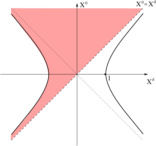
Figure 2: Upper-half the dS_d covered by our planar coordinates is given by shaded region.

Inserting these transformations (3.3) into the flat $(d+1)$-dimensional Minkowski metric (3.6), we obtain a familiar form of the planar metric of the dS_d :

$$ds^{2}=-d{\sf t}^{2}+e^{2{\sf t}/l}d{x^{i}}^{2}$$ (3.62)

which coincides exactly with the flat solution (3.58) found by solving the Einstein equations (3.54)–(3.55).

Since the metric (3.62) is not isometric under time translation, $\partial/\partial{\sf t}$ is not a timelike Killing vector. This nonexistence implies no notion of conserved energy and Hamiltonian, which hinders description of quantum gravity in the planar coordinates. However, the metric (3.62) is independent of $x^{i}$, so it satisfies form-invariance (3.1). Therefore, $\partial/\partial x^{i}$’s are spacelike Killing vectors and the spatial geometry involves translational symmetries and rotational symmetries.

3.4 Static coordinates $(t,r,\theta_{a}),~{}a=1,2,\cdots,d-2$

The constraint of the hyperboloid (3.5) embedded in $(d+1)$-dimensional Minkowski spacetime is again decomposed into two constraints by introducing an additional parameter $r$, of which one is a 2-dimensional hyperbola of radius $\sqrt{1-\left(r/l\right)^{2}}$

$$-\left({\frac{X^{0}}{l}}\right)^{2}+\left({\frac{X^{d}}{l}}\right)^{2}=1-\left({\frac{r}{l}}\right)^{2}$$ (3.63)

and the other is a $(d-1)$-dimensional sphere of radius $r/l$

$$-\left({\frac{X^{1}}{l}}\right)^{2}+\cdots+\left({\frac{X^{d-1}}{l}}\right)^{2}=\left({\frac{r}{l}}\right)^{2}.$$ (3.64)

Therefore, a nice coordinate system to implement the above two constraints (3.63)–(3.64) is

$$\frac{X^{0}}{l} = -\sqrt{1-\left(\frac{r}{l}\right)^{2}}\sinh\frac{t}{l},$$

$$\frac{X^{i}}{l} = \frac{r}{l}\omega^{i},~{}~{}~{}~{}~{}(i=1,2,\cdots,d-1),$$

$$\frac{X^{d}}{l} = -\sqrt{1-\left(\frac{r}{l}\right)^{2}}\cosh\frac{t}{l},$$ (3.65)

where $\omega^{i}$’s were given in Eq. (3.1) and $r~{}(0\leq r<\infty)$ will be identified with radial coordinate of static coordinate system. Since $-X^{0}+X^{d}=-\sqrt{l^{2}-r^{2}}\exp(-{\sf t}/l)\leq 0$ and $X^{0}+X^{d}=-\sqrt{l^{2}-r^{2}}\exp({\sf t}/l)\leq 0$, the region of $r\leq l$ covers only a quarter of the whole dS_d as shown by the shaded region in Fig. 3. Later, $r=l$ will be identified by a horizon of the pure de Sitter spacetime.

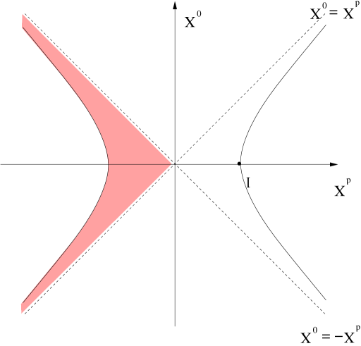
Figure 3: The region bounded by the de Sitter horizon $(r\leq l)$ is shown by shaded region.

Inserting these transformations (3.4) into the $(d+1)$-dimensional Minkowski metric (3.6), we obtain a familiar form of static metric of the dS_d :

$$ds^{2}=-\left[1-\left(\frac{r}{l}\right)^{2}\right]dt^{2}+\frac{dr^{2}}{\left[1-\left(\frac{r}{l}\right)^{2}\right]}+r^{2}d\Omega^{2}_{d-2},$$ (3.66)

where

$$d\Omega^{2}_{d-2} = d\theta_{1}^{2}+\sin^{2}\theta_{1}d\theta_{2}^{2}+\cdots+\sin^{2}\theta_{1}\cdots\sin^{2}\theta_{d-3}d\theta^{2}_{d-2}$$

$$= \sum_{b=1}^{d-2}\left(\prod_{a=1}^{b-1}\sin^{2}\theta_{a}\right)d\theta_{b}^{2}.$$

The metric (3.66) is form-invariant (3.1) for both time translation and rotation of the coordinate $\theta_{d-2}$ so that we have two Killing vectors, $\partial/\partial t$ and $\partial/\partial\theta_{d-2}$. Correspondingly, spacetime geometry has axial and time translational symmetries. Therefore, Hamiltonian is well-defined in the static coordinates (3.66) but unitarity is threatened by existence of the horizon at $r=l$.

In order to describe the system with rotational symmetry in $d$-dimensions, a static observer may introduce the static coordinate system where the metric involves two independent functions of the radial coordinate $r$, e.g., $\Omega(r)$ and $A(r)$ :

$$ds^{2}=-e^{2\Omega(r)}A(r)dt^{2}+\frac{dr^{2}}{A(r)}+r^{2}d\Omega^{2}_{d-2}.$$ (3.67)

Curvature scalar of the metric (3.67) is computed as

$$R=(d-2)\left[\frac{(d-3)(1-A)}{r^{2}}-\frac{2}{r}\left(\frac{dA}{dr}+A\frac{d\Omega}{dr}\right)\right]-\left[\frac{d^{2}A}{dr^{2}}+2A\frac{d^{2}\Omega}{dr^{2}}+2A\left(\frac{d\Omega}{dr}\right)^{2}+3\frac{dA}{dr}\frac{d\Omega}{dr}\right].$$ (3.68)

From Eqs. (A.25) and (A.26), simplified form of the Einstein equations (2.6) is

$$\frac{d-2}{r}\frac{d\Omega}{dr}=0,$$ (3.69)

$$\frac{d-2}{r^{d-2}}\frac{d}{dr}\left[r^{d-3}(1-A)\right]=\frac{(d-1)(d-2)}{l^{2}}.$$ (3.70)

Schwarzschild-de Sitter solution of Eqs. (3.69) and (3.70) is

$$\Omega=\Omega_{0}~{}~{}\mbox{and}~{}~{}A=1-\frac{r^{2}}{l^{2}}-\frac{2GM}{r^{d-3}}.$$ (3.71)

Here an integration constant $\Omega_{0}$ can always be absorbed by a scale transformation of the time variable $t$, $dt\rightarrow e^{-\Omega_{0}}dt$, and the other integration constant $M$ is chosen to be zero for the pure de Sitter spacetime of our interest, which is proportional to the mass of a Schwarzschild-de Sitter black hole [12]. Then the resultant metric coincides exactly with that of Eq. (3.66).

4 Geodesics

Structure of a fixed curved spacetime is usually probed by classical motions of a test particle. The shortest curve, the geodesic, connecting two points in the de Sitter space is determined by a minimum of its arc-length $\sigma$ for given initial point $P_{\rm i}$ and end-point $P_{\rm f}$, and is parametrized by an arbitrary parameter $\lambda$ such as $x^{\mu}(\lambda)$ :

$$\sigma=\int_{P_{\rm i}}^{P_{\rm f}}d\sigma=\int_{\lambda_{\rm i}}^{\lambda_{\rm f}}d\lambda\,\frac{dI}{d\lambda}=\int_{\lambda_{\rm i}}^{\lambda_{\rm f}}d\lambda\,L=\int_{\lambda_{\rm i}}^{\lambda_{\rm f}}d\lambda\,\sqrt{g_{\mu\nu}\frac{dx^{\mu}}{d\lambda}\frac{dx^{\nu}}{d\lambda}}=({\rm extremum}).$$ (4.1)

According to the variational principle, the geodesic must obey second-order Euler-Lagrange equation

$$\frac{d^{2}x^{\mu}}{d\lambda^{2}}+\Gamma^{\mu}_{\nu\rho}\frac{dx^{\nu}}{d\lambda}\frac{dx^{\rho}}{d\lambda}=0.$$ (4.2)

When the parameter $\lambda$ is chosen by the arc-length $\sigma$ itself, a force-free test particle moves on a geodesic.

In this section, we analyze precisely possible geodesics in the four coordinate systems of the de Sitter spacetime, obtained in the previous section. We also introduce several useful quantities in each coordinate system and explain some characters of the obtained geodesics.

4.1 Global (closed) coordinates

Lagrangian for the geodesic motions (4.1) is read from the metric (3.19) in the global coordinates :

$$L^{2}=-\left(\frac{d\tau}{d\lambda}\right)^{2}+l^{2}\cosh^{2}\left(\frac{\tau}{l}\right)\sum_{j=1}^{d-1}\left(\prod_{i=1}^{j-1}\sin^{2}\theta_{i}\right)\left(\frac{d\theta_{j}}{d\lambda}\right)^{2},$$ (4.3)

where $\lambda$ is an affine parameter. Corresponding geodesic equations (4.2) are given by $d$-coupled equations

$$\frac{d^{2}\tau}{d\lambda^{2}}+l\sinh(\tau/l)\cosh(\tau/l)\prod_{j=1}^{i-1}\sin^{2}\theta_{j}\left(\frac{d\theta_{i}}{d\lambda}\right)^{2}=0\;,$$ (4.4)

$$\frac{d^{2}\theta_{i}}{d\lambda^{2}}+\frac{2}{l}\frac{\sinh(\tau/l)}{\cosh(\tau/l)}\frac{d\tau}{d\lambda}\frac{d\theta_{i}}{d\lambda}-\sin\theta_{i}\cos\theta_{i}\prod_{j=i+1}^{j-1}\sin^{2}\theta_{j}\left(\frac{d\theta_{j}}{d\lambda}\right)^{2}+2\left(\sum_{k=1}^{i-1}\frac{\cos\theta_{k}}{\sin\theta_{k}}\frac{d\theta_{k}}{d\lambda}\right)\frac{d\theta_{j}}{d\lambda}=0\;.$$ (4.5)

Since $\theta_{d-1}$ is cyclic, $d\theta_{d-1}/d\lambda$ in Eq. (4.5) is replaced by a constant of motion $J$ such as

$$l^{2}\cosh^{2}(\tau/l)\prod_{j=1}^{i-1}\sin^{2}\theta_{j}\frac{d\theta_{d-1}}{d\lambda}=J.$$ (4.6)

Let us recall a well-known fact that any geodesic connecting arbitrary two points on a $(d-1)$-dimensional sphere should be located on its greatest circle. Due to rotational symmetry on the $S^{d-1}$, one can always orient the coordinate system so that the radial projection of the orbit coincides with the equator,

$$\theta_{1}=\theta_{2}=\theta_{3}=\cdots=\theta_{d-2}=\frac{\pi}{2},$$ (4.7)

of the spherical coordinates. This can also be confirmed by an explicit check that Eq. (4.7) should be a solution of Eq. (4.5). It means that a test particle has at start and continues to have zero momenta in the $\theta_{i}$-directions ($i=1,2,\cdots,d-2$). Therefore, the system of our interest reduces from $d$-dimensions to ($1+1$)-dimensions without loss of generality. Insertion of Eq. (4.7) into Eq. (4.6) gives

$$\frac{d\theta_{d-1}}{d\lambda}=\frac{J}{l^{2}\cosh^{2}(\tau/l)},$$ (4.8)

so that the remaining equation (4.4) becomes

$$\frac{d^{2}\tau}{d\lambda^{2}}=-\frac{J^{2}}{l^{3}}\frac{\sinh(\tau/l)}{\cosh^{3}(\tau/l)}.$$ (4.9)

Integration of Eq. (4.9) arrives at the conservation of ‘energy’ $E$

$$E=\frac{1}{2}\left(\frac{d\tau}{d\lambda}\right)^{2}+V_{\rm eff}(\tau/l),$$ (4.10)

where the effective potential $V_{\rm eff}$ is given by

$$V_{\rm eff}(\tau/l)=\left\{\begin{array}[]{cl}0&(J=0)\\ -\frac{1}{2}\left(\frac{J}{l}\right)^{2}\frac{1}{\cosh^{2}(\tau/l)}&(J\neq 0)\end{array},\right.$$ (4.11)

and thereby another constant of motion $E$ should be bounded below, i.e., $E\geq-\frac{1}{2}(J/2l)^{2}$. Eliminating the affine parameter $\lambda$ in both Eq. (4.8) and Eq. (4.10), we obtain the orbit equation which is integrated as an algebraic equation :

$$\tan\theta_{d-1}=\frac{J}{l}\frac{\sinh{(\tau/l)}}{\sqrt{(J/l)^{2}+2E\cosh^{2}(\tau/l)}}.$$ (4.12)

Since the spatial sections are sphere $S^{d-1}$ of a constant positive curvature and Cauchy surfaces, their geodesic normals of $J=0$ are lines which monotonically contract to a minimum spatial separation and then re-expand to infinity (See dotted line in Fig. 4). Another representative geodesic motion of $J\neq 0$ (dashed line) is also sketched in Fig. 4. For example, suppose that the affine parameter $\lambda$ is identified with the coordinate time $\tau$. Then, we easily confirm from the above analysis that every geodesic emanating from any point can be extended to infinite values of the affine parameters in both directions, $\lambda=\tau\in(-\infty,\infty)$, so that the de Sitter spacetime is said to be geodesically complete. However, there exist spatially-separated points which cannot be joined by one geodesic.

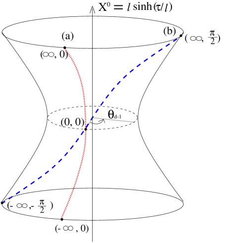
Figure 4: Two representative geodesic motions in the global coordinates : (a) dotted line for $J=0$, (b) dashed line for $J\neq 0$.

4.2 Conformal coordinates

Similar to the procedure in the previous subsection, we read automatically Lagrangian for geodesics (4.1) from the conformal metric (3.35) :

$$L^{2}=\sec^{2}\left(\frac{T}{l}\right)\left[-\left(\frac{dT}{d\lambda}\right)^{2}+l^{2}\sum_{j=1}^{d-1}\left(\prod_{i=1}^{j-1}\sin^{2}\theta_{i}\right)\left(\frac{d\theta_{j}}{d\lambda}\right)^{2}\right],$$ (4.13)

and then corresponding geodesic equations (4.2) are

$$\frac{d^{2}T}{d\lambda^{2}}+\frac{1}{l}\frac{\sin(T/l)}{\cos(T/l)}\left(\frac{dT}{d\lambda}\right)^{2}+l\frac{\sin(T/l)}{\cos(T/l)}\prod_{j=1}^{i-1}\sin^{2}\theta_{j}\left(\frac{d\theta_{i}}{d\lambda}\right)^{2}=0\;,$$ (4.14)

$$\frac{d^{2}\theta_{i}}{du^{2}}+\frac{2}{l}\frac{\sin(T/l)}{\cos(T/l)}\frac{dT}{d\lambda}\frac{d\theta_{i}}{d\lambda}-\sin\theta_{i}\cos\theta_{i}\prod_{j=i+1}^{j-1}\sin^{2}\theta_{j}\left(\frac{d\theta_{j}}{d\lambda}\right)^{2}+2\left(\sum_{k=1}^{i-1}\frac{\cos\theta_{k}}{\sin\theta_{k}}\frac{d\theta_{k}}{d\lambda}\right)\frac{d\theta_{j}}{d\lambda}=0\;.$$ (4.15)

Since $\theta_{d-1}$ is cyclic, $d\theta_{d-1}/d\lambda$ is replaced by a constant of motion $J$ such as

$$l^{2}\cos^{-2}(T/l)\prod_{j=1}^{i-1}\sin^{2}\theta_{j}\frac{\theta_{d-1}}{d\lambda}=J.$$ (4.16)

Since the $(d-1)$-angular coordinates $\{\theta_{i}\}$ constitute a ($d-1$)-dimensional sphere, the same argument around Eq. (4.7) is applied and thereby the system of our interest reduces again from $d$-dimensions to $(1+1)$-dimensions without loss of generality. Substituting of Eq. (4.7) into Eq. (4.16), we have

$$\frac{d\theta_{d-1}}{d\lambda}=\frac{J}{l^{2}}\cos^{2}(T/l)$$ (4.17)

and rewrite Eq. (4.14) as

$$\frac{d^{2}T}{d\lambda^{2}}+\frac{1}{l}\tan(T/l)\left(\frac{dT}{d\lambda}\right)^{2}+l\tan(T/l)\left(\frac{d\theta_{d-1}}{d\lambda}\right)^{2}=0\;.$$ (4.18)

Eq. (4.18) is integrated out and we obtain another conserved quantity $E$ :

$$E\equiv-\frac{l^{2}}{2}\left(\frac{d\theta_{d-1}}{d\lambda}\right)^{2}=\frac{1}{2}\left(\frac{dT}{d\lambda}\right)^{2}-\cos^{2}(T/l)\;.$$ (4.19)

In Eq. (4.19) we rescaled the affine parameter $\lambda$ in order to absorb a redundant constant. Combining Eq. (4.17) and Eq. (4.19), we obtain an orbit equation expressed by elliptic functions :

$$\theta_{d-1}=\frac{J}{l\sqrt{2}}\left[\sqrt{1+E}\,EllipticE\left(\frac{T}{l},\frac{1}{E+1}\right)-\frac{E}{\sqrt{1+E}}\,EllipticF\left(\frac{T}{l},\frac{1}{E+1}\right)\right]\;,$$ (4.20)

where

$$EllipticE\left(\frac{T}{l},\frac{1}{E+1}\right)=\int dT\sqrt{1-\frac{1}{E+1}\sin^{2}(T/l)}\;,$$ (4.21)

$$EllipticF\left(\frac{T}{l},\frac{1}{E+1}\right)=\int dT\frac{1}{\sqrt{1-\frac{1}{E+1}\sin^{2}(T/l)}}\;.$$ (4.22)

($T,\theta_{d-1}$) represents a cylinder of finite height as shown in Fig. 5. Geodesic of zero energy, $E=0$, (or equivalently zero angular momentum, $J=0$), is shown as a dotted line, and that of positive energy, $E>0$, (or nonvanishing angular momentum, $J\neq 0$), as a dashed line in Fig. 5.

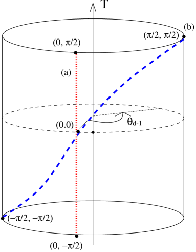
Figure 5: Geodesics on the $(T,\theta_{d-1})$ plane : (a) dotted line for $J=0$, (b) dashed line for $J\neq 0$.

4.3 Planar (inflationary) coordinates

Lagrangian for the geodesic motion (4.1) for the flat space of $k=0$ is read from the metric (3.53) :

$$L^{2}=-\left(\frac{d{\sf t}}{d\lambda}\right)^{2}+e^{2{\sf t}/l}\left(\frac{d{\sf r}}{d\lambda}\right)^{2}+e^{2{\sf t}/l}{\sf r}^{2}\sum_{b=1}^{d-2}\left(\prod_{a=1}^{b-1}\sin^{2}\theta_{a}\right)\left(\frac{d\theta_{b}}{d\lambda}\right)^{2},$$ (4.23)

and the corresponding geodesic equations (4.2) are

$$\frac{d^{2}\sf t}{d\lambda^{2}}+\frac{1}{l}e^{2{\sf t}/l}\left(\frac{d{\sf r}}{d\lambda}\right)^{2}+\frac{e^{2{\sf t}/l}}{l}{\sf r}^{2}\sum_{b=1}^{d-2}\left(\prod_{a=1}^{b-1}\sin^{2}\theta_{a}\right)\left(\frac{d\theta_{b}}{d\lambda}\right)^{2}=0\;,$$ (4.24)

$$\frac{d^{2}{\sf r}}{d\lambda^{2}}+\frac{2}{l}\frac{d\sf t}{d\lambda}\frac{d{\sf r}}{d\lambda}-{\sf r}\sum_{b=1}^{d-2}\left(\prod_{a=1}^{b-1}\sin^{2}\theta_{a}\right)\left(\frac{d\theta_{b}}{d\lambda}\right)^{2}=0\;,$$ (4.25)

$$\frac{d^{2}\theta_{a}}{d\lambda^{2}}+\frac{2}{l}\frac{d{\sf t}}{d\lambda}\frac{d\theta_{a}}{d\lambda}+\frac{2}{{\sf r}}\frac{d{\sf r}}{d\lambda}\frac{d\theta_{a}}{d\lambda}-\sin\theta_{a}\cos\theta_{a}\prod_{b=a+1}^{b-1}\sin^{2}\theta_{b}\left(\frac{d\theta_{b}}{d\lambda}\right)^{2}+2\left(\sum_{c=1}^{a-1}\frac{\cos\theta_{c}}{\sin\theta_{c}}\frac{d\theta_{c}}{d\lambda}\right)\frac{d\theta_{b}}{d\lambda}=0\;.$$ (4.26)

Since $\theta_{d-2}$ is cyclic, $d\theta_{d-2}/d\lambda$ is replaced by a constant of motion $J$ such as

$$2e^{2{\sf t}/l}{\sf r}^{2}\prod_{b=1}^{d-3}\sin^{2}\theta_{b}\frac{d\theta_{d-2}}{d\lambda}=J.$$ (4.27)

If we use a well-known fact that any geodesic connecting arbitrary two points on a $(d-2)$-dimensional sphere should be located on its greatest circle, one may choose without loss of generality

$$\theta_{1}=\theta_{2}=\theta_{3}=\cdots=\theta_{d-3}=\frac{\pi}{2},$$ (4.28)

which should be a solution of Eq. (4.26) due to rotational symmetry on the $(d-2)$-dimensional sphere $S^{d-2}$. Therefore, the system of our interest reduces from $d$-dimensions to $(2+1)$-dimensions without loss of generality.
Insertion of Eq. (4.28) into Eq. (4.27) gives

$$\frac{d\theta_{d-2}}{d\lambda}=\frac{J}{2e^{2{\sf t}/l}{\sf r}^{2}},$$ (4.29)

so that the equations (4.24)–(4.25) become

$$\frac{d^{2}\sf t}{d\lambda^{2}}+\frac{e^{2{\sf t}/l}}{l}\left(\frac{d{\sf r}}{d\lambda}\right)^{2}+\frac{J^{2}}{4l}\frac{e^{-2{\sf t}/l}}{{\sf r}^{2}}=0\;,$$ (4.30)

$$\frac{d^{2}{\sf r}}{d\lambda^{2}}+\frac{2}{l}\frac{d\sf t}{d\lambda}\frac{d{\sf r}}{d\lambda}-\frac{J^{2}}{4}\frac{e^{-4{\sf t}/l}}{{\sf r}^{3}}=0\;.$$ (4.31)

Eliminating the third term in both Eqs. (4.30)–(4.31) by subtraction, we have the combined equation

$${\sf r}\frac{d{\sf r}}{d\lambda}e^{2{\sf t}/l}=-l\frac{d{\sf t}}{d\lambda}+C,$$ (4.32)

where $C$ is constant. Finally, for $C=0$, the radial equation (4.32) is solved as

$${\sf r}=le^{{\sf-t}/l}.$$ (4.33)

For $J=0$, Eq. (4.31) becomes

$$\frac{d}{d\lambda}\left(2e^{2{\sf t}/l}\frac{d{\sf r}}{d\lambda}\right)=0.$$ (4.34)

It reduces $dr/d\lambda=C^{\prime}e^{-2{\sf t}/l}$ and $C^{\prime}$ is constant.

Information on the scale factor $a({\sf t})$ is largely gained through the observation of shifts in wavelength of light emitted by distant sources. It is conventionally gauged in terms of redshift parameter $z$ between two events, defined as the fractional change in wavelength :

$$z\equiv\frac{\lambda_{0}-\lambda_{1}}{\lambda_{1}},$$ (4.35)

where $\lambda_{0}$ is the wavelength observed by us here after long journey and $\lambda_{1}$ is that emitted by a distant source. For convenience, we place ourselves at the origin ${\sf r}=0$ of coordinates since our de Sitter space is homogeneous and isotropic, and consider a photon traveling to us along the radial direction with fixed $\theta_{a}$’s. Suppose that a light is emitted from the source at time ${\sf t}_{1}$ and arrives at us at time ${\sf t}_{0}$. Then, from the metric (3.53), the null geodesic connecting (${\sf t}_{1},{\sf r}_{1},\theta_{1},\cdots,\theta_{d-2}$) and (${\sf t}_{0},0,\theta_{1},\cdots,\theta_{d-2}$) relates coordinate time and distance as follows

$$\int^{{\sf t}_{0}}_{{\sf t}_{1}}\frac{d{\sf t}}{a(\sf t)}=\int^{{\sf r}_{1}}_{0}\frac{d{\sf r}}{\sqrt{1-k{\sf r}^{2}}}\equiv f({\sf r}_{1}).$$ (4.36)

If next wave crest leaves ${\sf r}_{1}$ at time ${\sf t}_{1}+\delta{\sf t}_{1}$ and reach us at time ${\sf t}_{0}+\delta{\sf t}_{0}$, the time independence of $f({\sf r}_{1})$ provides

$$\int^{{\sf t}_{1}+\delta{\sf t}_{1}}_{{\sf t}_{1}}\frac{d{\sf t}}{a({\sf t})}=\int^{{\sf t}_{0}+\delta{\sf t}_{0}}_{{\sf t}_{0}}\frac{d{\sf t}}{a({\sf t})}.$$ (4.37)

For sufficiently short time $\delta{\sf t}_{0}$ (or $\delta{\sf t}_{1}$) the scale factor $a({\sf t})$ is approximated by a constant over the integration time in Eq. (4.37), and, with the help of $\lambda_{0}=\delta{\sf t}_{0}\ll|{\sf t}_{1}-{\sf t}_{0}|$ (or $\lambda_{1}=\delta{\sf t}_{1}\ll|{\sf t}_{1}-{\sf t}_{0}|$), Eq. (4.37) results in

$$\frac{\lambda_{1}}{\lambda_{0}} = \frac{a({\sf t}_{1})}{a({\sf t}_{0})}$$ (4.38)

$$= 1+H_{0}({\sf t}_{1}-{\sf t}_{0})-\frac{1}{2}q_{0}H^{2}_{0}({\sf t}_{1}-{\sf t}_{0})^{2}+\cdots\,,$$ (4.39)

where $H_{0}=H({\sf t}_{0})$ from Eq. (3.57) and $q_{0}=q({\sf t}_{0})$ from Eq (3.56). Substituting Eq. (4.38) into Eq. (4.35), we have

$$z=\frac{a({\sf t}_{0})}{a({\sf t}_{1})}-1.$$ (4.40)

On the other hand, the comoving distance ${\sf r}_{1}$ is not measurable so that we can define the luminosity distance $d_{L}$ :

$$d_{L}^{2}\equiv\frac{L}{4\pi F},$$ (4.41)

where $L$ is absolute luminosity of the source and $F$ is flux measured by the observer. It is motivated from the fact that the measured flux $F$ is simply equal to luminosity times one over the area around a source at distance $d$ in flat space. In expanding universe, the flux will be diluted by the redshift of the light by a factor $(1+z)$ and the difference between emitting time and measured time. When comoving distance between the observer and the light source is ${\sf r}_{1}$, a physical distance $d$ becomes $a_{0}r_{1}$, where $a_{0}$ is scale factor when the light is observed. Therefore, we have

$$\frac{F}{L}=\frac{1}{4\pi a_{0}^{2}r_{1}^{2}(1+z)^{2}}.$$ (4.42)

Inserting Eq. (4.42) into Eq. (4.41), we obtain

$$d_{L}=a_{0}r_{1}(1+z).$$ (4.43)

Using the expansion (4.39), Eq. (4.40) is expressed by

$$\frac{1}{1+z}=1+H_{0}({\sf t}_{1}-{\sf t}_{0})-\frac{1}{2}q_{0}H^{2}_{0}({\sf t}_{1}-{\sf t}_{0})^{2}+\cdots.$$ (4.44)

For small $H_{0}({\sf t}_{1}-{\sf t}_{0})$, Eq. (4.44) can be inverted to

$${\sf t}_{0}-{\sf t}_{1}=H_{0}^{-1}\left[z-\left(1+\frac{q_{0}}{2}\right)z^{2}+\cdots\right].$$ (4.45)

When $k=0$, the right-hand side of Eq. (4.36) yields ${\sf r}$ and expansion of the left-hand side for small $H_{0}({\sf t}_{1}-{\sf t}_{0})$ gives

$${\sf r}_{1} = \int^{{\sf t}_{0}}_{{\sf t}_{1}}d{\sf t}\left(\frac{1}{a({\sf t}_{1})}-\frac{\dot{a}({\sf t}_{1})}{a^{2}({\sf t}_{1})}{\sf t}+\cdots\right)$$ (4.46)

$$= \frac{1}{a_{0}}\left[({\sf t}_{0}-{\sf t}_{1})+\frac{1}{2}H_{0}({\sf t}_{0}-{\sf t}_{1})^{2}+\cdots\right]$$

$$= \frac{1}{a_{0}H_{0}}\left[z-\frac{1}{2}(1+q_{0})z^{2}+\cdots\right],$$

where $a({\sf t}_{1})\approx a_{0}+\dot{a}_{0}({\sf t}_{1}-{\sf t}_{0})+\frac{1}{2}\ddot{a}_{0}({\sf t}_{1}-{\sf t}_{0})^{2}+\cdots$ was used in the second line and Eq. (4.45) was inserted in the third line. Replacing ${\sf r}_{1}$ in Eq. (4.43) by Eq. (4.46), we finally have Hubble’s law :

$$d_{L}=H_{0}^{-1}\left[z+\frac{1}{2}(1-q_{0})z^{2}+\cdots\right]$$ (4.47)

which relates the distance to a source with its observed red shift. Note that we can determine present Hubble parameter $H_{0}$ and present deceleration parameter $q_{0}$ by measurement of the luminosity distances and redshifts. As a reference, observed value of $H_{0}$ at present is $H_{0}=100{\rm h\,km/s\,Mpc}$ ($0.62\stackrel{{\scriptstyle<}}{{{}_{\sim}}}h\stackrel{{\scriptstyle<}}{{{}_{\sim}}}0.82$) so that corresponding time scale $T_{\rm universe}\equiv H_{0}^{-1}$ is about one billion year and length scale $L_{\rm universe}\equiv cH_{0}^{-1}$ is about several thousand ${\rm Mpc}$. Since the scale factor is given by an exponential function, $a({\sf t})=e^{{\sf t}/l}$, for the flat spacetime of $k=0$, the left-hand side of Eq. (4.36) is integrated in a closed form :

$$\frac{{\sf r}_{1}}{l}=e^{-{\sf t}_{1}/l}-e^{-{\sf t}_{0}/l}.$$ (4.48)

In addition, the redshift parameter $z$ is expressed as

$$z=e^{({\sf t}_{0}-{\sf t}_{1})/l}-1,$$ (4.49)

so the luminosity distance $d_{L}$ in Eq. (4.43) becomes

$$d_{L}=l(z+z^{2}).$$ (4.50)

Comparing Eq. (4.50) with the Hubble’s law (4.47), we finally confirm that the expanding flat space solution of $k=0$ has present Hubble parameter $H_{0}=1/l$ and the de Sitter universe is accelerating with present deceleration parameter $q_{0}=-1$ as expected.

4.4 Static coordinates

Geodesic motions parametrized by proper time $\sigma$ are described by the following Lagrangian read from the static metric (3.66) :

$$L^{2}=-\left[1-\left(\frac{r}{l}\right)^{2}\right]\left(\frac{dt}{d\sigma}\right)^{2}+\frac{1}{1-\left(\frac{r}{l}\right)^{2}}\left(\frac{dr}{d\sigma}\right)^{2}+r^{2}\sum_{b=1}^{d-2}\left(\prod_{a=1}^{b-1}\sin^{2}\theta_{a}\right)\left(\frac{d\theta_{b}}{d\sigma}\right)^{2}.$$ (4.51)

Since the time $t$ and angle $\theta_{d-2}$ coordinates are cyclic, the conjugate momenta $E$ and $J$ are conserved :

$$J\equiv\frac{\partial L^{2}}{\partial\left(\frac{d\theta_{d-2}}{d\sigma}\right)}=r^{2}\prod_{j=1}^{d-3}\sin^{2}\theta_{j}\frac{d\theta_{d-2}}{d\sigma}\;,$$ (4.52)

$$\sqrt{-2E}\equiv\frac{\partial L^{2}}{\partial\left(\frac{dt}{d\sigma}\right)}=-\left[1-\left(\frac{r}{l}\right)^{2}\right]\frac{dt}{d\sigma}\;.$$ (4.53)

By the same argument in the subsection 4.3, the system of our interest reduces from $d$-dimensions to ($2+1$)-dimensions without loss of generality, and then Eq. (4.52) becomes

$$\frac{d\theta_{d-2}}{d\sigma}=\frac{J}{r^{2}}\;.$$ (4.54)

From here on let us use rescaled variables $e=E/l^{2}$, $x=r/l$, and $j=J/l^{2}$. Note that $j$ cannot exceed $1$ due to the limitation of light velocity. Then second-order radial geodesic equation from the Lagrangian (4.51) becomes

$$\frac{d^{2}x}{d\sigma^{2}}+\frac{x}{1-x^{2}}\left(\frac{dx}{d\sigma}\right)^{2}+2e\frac{x}{1-x^{2}}-j^{2}\frac{1-x^{2}}{x^{3}}=0.$$ (4.55)

Integration of Eq. (4.55) leads to conservation of the energy $e$

$$e=\frac{1}{2}\left(\frac{dx}{d\sigma}\right)^{2}+\frac{V_{\rm eff}}{l^{2}}\leq 0\;,$$ (4.56)

where the effective potential $V_{\rm eff}$ is given by

$$V_{\rm eff}(x)=\frac{l^{2}}{2}\left(1-x^{2}\right)\left(\frac{j^{2}}{x^{2}}-1\right)\;.$$ (4.57)

As shown in Fig. 6, the motion of a particle having the energy $e_{1}$ can never lower than $x=j$ due to repulsive centrifugal force, which becomes $0$ as $j$ approaches $0$. The ranges except $j<r<1$ are forbidden by the fact that kinetic energy should be positive. For $e=e_{2}$ indicated in Fig. 6, a test particle moves bounded orbit within two turning points $x_{1}$ and $x_{2}$. The perihelion $x_{1}$ and the aphelion $x_{2}$ were obtained from $dx/d\sigma=0$

$$x_{1}^{2} = \frac{j^{2}+1+2e-\sqrt{(j^{2}+1+2e)^{2}-4j^{2}}}{2},$$

$$x_{2}^{2} = \frac{j^{2}+1+2e+\sqrt{(j^{2}+1+2e)^{2}-4j^{2}}}{2}.$$ (4.58)

If the energy $e$ have minimum value of the effective potential $e=e_{3}$, then the motion is possible only at $x=x_{0}$, so that the orbital motion should be circular.

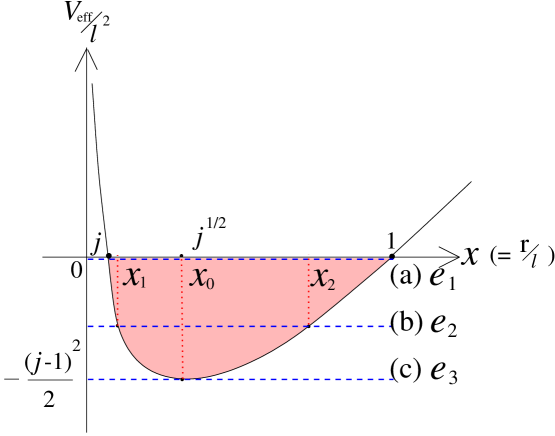
Figure 6: Effective potential and various available values of the energy $e$ : (a) $e_{1}=0$, (b) $-\frac{(j-1)^{2}}{2}<e_{2}<0$, (c) $e_{3}=-\frac{(j-1)^{2}}{2}$.

Shaded region in Fig. 6 is the allowable region for static observer, which is bounded by de Sitter horizon ($x=1$). It corresponds to one fourth of the global hyperbolic region in Fig. 9.

Solving for $dr/d\sigma$ from Eq. (4.56), we have

$$d\sigma=\frac{dx^{2}}{2\sqrt{-x^{4}+(j^{2}+2e+1)x^{2}-j^{2}}}.$$ (4.59)

Then the integration of both sides gives

$$x^{2}=\frac{j^{2}+1+2e}{2}+\frac{1}{2}\sqrt{(j^{2}+1+2e)^{2}-4j^{2}}\sin{(2\sigma+C)},$$ (4.60)

where $C$ is an integration constant. If we choose the perihelion $x_{1}$ given in Eq. (4.4) for $\sigma=0$, $C$ is fixed by $-\pi/2$ and then the aphelion $x_{2}$ is given at $\sigma=\pi/2$. When the energy $e$ takes maximum value $e=0$, position of the aphelion at $x=1$ is nothing but the de Sitter horizon. So the elapsed proper time for the motion from the perihelion to the aphelion, ($-\pi/2,\pi/2$), is finite.

Changing the proper time $\sigma$ in Eq. (4.59) to coordinate time of a static observer ${\sf t}$ by means of Eq. (4.53), we find

$$dt=dx^{2}\frac{\sqrt{-2e}}{(x^{2}-1)\sqrt{-x^{4}+(j^{2}+2e+1)x^{2}-j^{2}}},$$ (4.61)

and the integration for $e=e_{2}$ gives

$$\tan[2(t-t_{0})]=\frac{4e-(j^{2}-1+2e)(1-x^{2})}{\sqrt{-2e}(x^{2}-1)\sqrt{2e+(1-x^{2})(1-j^{2}/x^{2})}}.$$ (4.62)

Note that the ranges are

$$j<x<1,\;\;\;0<j<1,\;\;\;~{}$$

and

$$~{}-\frac{(j-1)^{2}}{2}<e_{2}<0.$$ (4.63)

In the case of $e=e_{1}$, the integration of Eq. (4.61) gives

$$t-t_{0}=\lim_{e\rightarrow 0}l\sqrt{-2e}\frac{\sqrt{(1-j^{2})(1-x^{2})-(1-x^{2})^{2}}}{(1-j^{2})(x^{2}-1)}.$$ (4.64)

To reach the de Sitter horizon at $x=1$, the energy $e$ should have a value $e_{1}$ irrespective of the value of $j$ as shown in Fig. 7. For $e=e_{3}=-(j-1)^{2}/2$, $x$ is fixed by $x_{0}=\sqrt{j}$. When a test particle approaches the de Sitter horizon, the elapsed coordinate time diverges as

$$t-t_{0} = \lim_{x\rightarrow 1^{-}}\frac{\sqrt{2}l}{1-j^{2}}\sqrt{\frac{1-j^{2}}{1-x^{2}}-1}$$ (4.65)

$$\sim \lim_{x\rightarrow 1^{-}}\frac{1}{\sqrt{1-x}}\rightarrow+\infty.$$

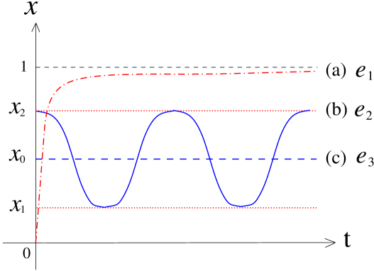
Figure 7: Radial geodesics on time $t$ : (a) dash-dot line for $e_{1}$, (b) solid line for $e_{2}$, (c) dashed line for $e_{3}$.

By combining Eq. (4.54) with Eq. (4.59) and its integration, we obtain an elliptic orbit equation for $e=e_{2}$ :

$$\sin(2\theta_{d-2}+\theta_{0})=\frac{-2j^{2}+(1+j^{2}+2e)x^{2}}{x^{2}\sqrt{[(1+j)^{2}+2e][(1-j)^{2}+2e]}}.$$ (4.66)

If we choose $x$ as the perihelion at $\theta_{d-2}=0$, $\theta_{0}$ becomes $-\pi/2$. From Eq. (4.4), the semimajor axis $a$ of $x^{2}$ is given by

$$a=\frac{x_{1}^{2}+x_{2}^{2}}{2}=\frac{j^{2}+1+2e}{2}.$$ (4.67)

Eccentricity $\varepsilon$ of the ellipse can be written

$$\varepsilon=\sqrt{1-\frac{j^{2}}{a^{2}}},$$ (4.68)

Dependence of the orbit for $\varepsilon$ is the followings :

$$\left\{\begin{array}[]{lll}\varepsilon<1,&\;\;\;e\leq 0:&{\rm ellipse},\\ \varepsilon=0,&\displaystyle\;\;\;e=-\frac{(j-1)^{2}}{2}:&{\rm circle}.\end{array}\right.$$ (4.69)

This scheme agrees with qualitative discussion by using the effective potential (4.57) and the energy diagram in Fig. 6. In terms of $A$ and $\varepsilon$, Eq. (4.66) is rewritten by

$$x=\sqrt{\frac{a(1-\varepsilon^{2})}{1+\varepsilon\cos(2\theta_{d-2})}}.$$ (4.70)

Eq. (4.70) follows $x=\sqrt{a(1-\varepsilon)}$ at $\theta_{d-2}=0$ and $x=\sqrt{a(1+\varepsilon)}$ at $\theta_{d-2}=\pi/2$ as expected from Eq. (4.4). As shown in Fig. 8, Eq. (4.70) satisfies the condition for closed orbits so-called Bertrand’s theorem, which means a particle retraces its own foot step.

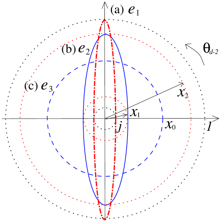
Figure 8: Orbits on ($x$, $\theta_{d-2}$)-plane : (a) dash-dot line for $e_{1}$, (b) solid line for $e_{2}$, (c) dashed line for $e_{3}$. Circles stand for de Sitter horizon, aphelion, circular orbit, two perihelia from the outside.

5 Penrose Diagram

Let us begin with a spacetime with physical metric $g_{\mu\nu}$, and introduce another so-called unphysical metric $\bar{g}_{\mu\nu}$, which is conformally related to $g_{\mu\nu}$ such as

$$\bar{g}_{\mu\nu}=\Omega^{2}g_{\mu\nu}.$$ (5.1)

Here, the conformal factor $\Omega$ is suitably chosen to bring in the points at infinity to a finite position so that the whole spacetime is shrunk into a finite region called Penrose diagram. A noteworthy property is that the null geodesics of two conformally related metrics coincide, which determine the light cones and, in turn, define causal structure. If such process called conformal compactification is accomplished, all the information on the causal structure of the de Sitter spacetime is easily visualized through this Penrose diagram although distances are highly distorted. In this section, we study detailed casual structure in various coordinates in terms of the Penrose diagram. Since every Penrose diagram is drawn as a two-dimensional square in the flat plane, each point in the diagram denotes actually a $(d-2)$-dimensional sphere $S^{d-2}$ except that on left or right side of the diagram.

5.1 Static coordinates

Let us introduce a coordinate transformation from the static coordinates (3.66) to Eddington-Finkelstein coordinates $(x^{+},~{}x^{-},~{}\theta_{a})$ such as

$$x^{\pm}\equiv t\pm\frac{l}{2}\ln\frac{1+\frac{r}{l}}{1-\frac{r}{l}},$$ (5.2)

where the range of $x^{\pm}$ is $(-\infty,\infty)$. As expected, $r/l=0$ results in a timelike curve for a static object at the origin, $x^{\pm}=t$. Then the metric in Eq. (3.66) becomes

$$ds^{2}=-{\rm sech}^{2}\left(\frac{x^{+}-x^{-}}{2l}\right)dx^{+}dx^{-}+l^{2}\tanh^{2}\left(\frac{x^{+}-x^{-}}{2l}\right)d\Omega_{d-2}^{2}.$$ (5.3)

Though the possible domain of real $r/l$ corresponds to the interior region of the de Sitter horizon [0,1) due to the logarithm of Eq. (5.2), the metric itself (5.3) remains to be real for the whole range of $r/l$ since $({\rm sech}[(x^{+}-x^{-})/2l],{\rm tanh}[(x^{+}-x^{-})/2l])$ has (1,0) at $r/l=0$, (0,1) at $r/l=1$, and $(-1,\infty)$ at $r/l=\infty$, so it covers the entire $d$-dimensional de Sitter spacetime as expected.

In order to arrive at Penrose diagram of our interest, these coordinates are transformed into Kruskal coordinates ($U$, $V$) by

$$U\equiv-e^{x^{-}/l}~{}\mbox{and}~{}V\equiv e^{-x^{+}/l},$$ (5.4)

and then the metric takes the form

$$ds^{2}=\frac{l^{2}}{(1-UV)^{2}}\left[-4dUdV+\left({1+UV}\right)^{2}d\Omega_{d-2}^{2}\right].$$ (5.5)

The value of $UV$ has $-1$ at the origin ($r/l=0$), $0$ at the horizon ($r/l=1$), and $1$ at infinity ($r/l=\infty$) by a relation $r/l=(1+UV)/(1-UV)$. In addition, another relation $-U/V=e^{2t/l}$ tells us that the line of $U=0$ corresponds to past infinity ($t=-\infty$) and $V=0$ does to future infinity ($t=\infty$). Therefore, the entire region of the de Sitter spacetime is drawn by a Penrose diagram which is a square bounded by $|UV|=1$. At the horizon, $r=l$ so that $r/l=(1+UV)/(1-UV)$ implies $UV=0$.

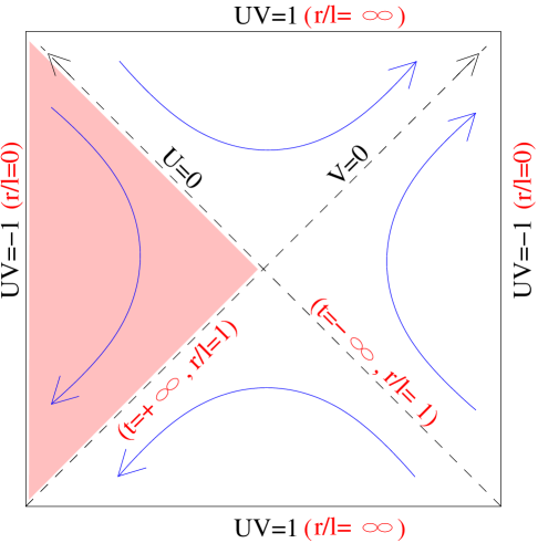
Figure 9: Penrose diagram of de Sitter spacetime from static coordinates.

Therefore, as shown in the Fig. 9, the coordinate axes $U=0$ and $V=0$ (dashed lines) are nothing but the horizons and the arrows on those dashed lines stand for the directions of increasing $U$ and $V$. The shaded region is the causally-connected region for the observer at the origin on the right-hand side of the square ($UV=-1$, $r/l=0$).

In the Kruskal coordinates (5.4), a Killing vector $\partial/\partial t$ in the static coordinates is expressed as

$$\frac{\partial}{\partial t}=\frac{U}{l}\frac{\partial}{\partial U}-\frac{V}{l}\frac{\partial}{\partial V}.$$ (5.6)

Thus norm of the Killing vector is

$$\left(\frac{\partial}{\partial t}\right)^{2}=4UV/(1-UV)^{2}.$$ (5.7)

Note that the norm of the Killing vector becomes null at $UV=0$. In the region of $UV>0$, the norm is spacelike, while a half of the region with negative $V$ is forbidden. Timelike Killing vector is defined only in the shaded region with $\left(\partial/\partial t\right)^{2}<0$ as shown in Fig. 9. Such existence of the Killing vector field $\partial/\partial t$ guarantees conserved Hamiltonian which allows quantum mechanical description of time evolution. However, $\partial/\partial t$ is spacelike in both top and bottom triangles and points toward the past in right triangle bounded by the southern pole in Fig. 9. Therefore, time evolution cannot be defined beyond the shaded region. The absence of global definition of timelike Killing vector in the whole de Sitter spacetime may predict difficulties in quantum theory, e.g., unitarity.

5.2 Conformal coordinates

As mentioned previously, the conformal metric (3.36) describes entire de Sitter spacetime and is flat except for a conformal factor $1/\cos^{2}(T/l)$ because of the scale symmetry (3.30). These properties are beneficial for drawing the Penrose diagram. By comparing the conformal metric (3.36) directly with that of the Kruskal coordinates (5.5), we obtain a set of coordinate transformation

$$U = \tan\left[\frac{1}{2}\left(\frac{T}{l}+\theta_{1}-\frac{\pi}{2}\right)\right],$$ (5.8)

$$V = \tan\left[\frac{1}{2}\left(\frac{T}{l}-\theta_{1}+\frac{\pi}{2}\right)\right],$$ (5.9)

where integration constants are chosen by considering easy comparison with the quantities in the static coordinates. Since the range of conformal time $T$ is $-\pi/2<T/l<\pi/2$, the horizontal slice $S^{d-1}$ at $T/l=-\pi/2\Leftrightarrow\tau/l=-\infty$ ($T/l=\pi/2\Leftrightarrow\tau/l=\infty$) forms a past (future) null infinity ${\cal I}^{-}$ (${\cal I}^{+}$) with $UV=1$ as shown in Fig. 10. When $\theta_{1}=0$ $(\theta_{1}=\pi)$, it is a vertical line on the left (right) side with $UV=-1$, which is called by north (south) pole. When $T/l=-\theta_{1}+\pi/2$ $({\rm or}\;T/l=\theta_{1}-\pi/2)$, $U=0$ $({\rm or}\;V=0)$ corresponding to a null geodesic (or another null geodesic) starts at the south (or north) pole at the past null infinity ${\cal I}^{-}$ and ends at the north (or south) pole at the future null infinity ${\cal I}^{+}$, where all null geodesics originate and terminate (See two dashed lines at $45$ degree angles in Fig. 10). Obviously, timelike surfaces are more vertical compared to the null geodesic lines and spacelike surfaces are more horizontal compared to those. Therefore, every horizontal slice of a constant $T$ is a surface $S^{d-1}$ and every vertical line of constant $\theta^{\prime}$s is timelike (See the horizontal and vertical lines in Fig. 10).

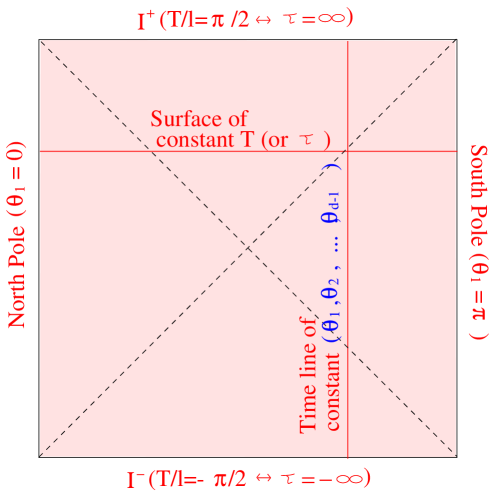
Figure 10: Penrose diagram of de Sitter spacetime in conformal coordinates.

Although this diagram contains the entire de Sitter spacetime, any observer cannot observe the whole spacetime. The de Sitter spacetime has particle horizon because past null infinity is spacelike, i.e., an observer at the north pole cannot see anything beyond his past null cone from the south pole at any time as shown by the region ${\cal O}^{-}$ in Fig. 11-(a), because the geodesics of particles are timelike. The de Sitter spacetime has future event horizon because future null infinity is also spacelike : The observer can never send a message to any region beyond ${\cal O}^{+}$ as shown in Fig. 11-(b). This fact is contrasted to the following from Minkowski spacetime where a timelike observer will eventually receive all history of the universe in the past light cone. Therefore, the fully accessible region to an observer at the north pole is the common region of both ${\cal O}^{-}$ and ${\cal O}^{+}$, which coincides exactly with the causally-connected region for the static observer at the origin in Fig. 9.

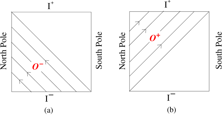
Figure 11: (a) Causal past of an observer at the north pole (b) Causal future of an observer at the north pole

5.3 Planar (inflationary) coordinates

By comparing the planar coordinates (3.62) with the Kruskal coordinates (5.5), we again find a set of coordinate transformation

$$U = \frac{{\sf r}/l-e^{{-\sf t}/l}}{2},$$ (5.10)

$$V = \frac{2}{e^{{-\sf t}/l}+{\sf r}/l}.$$ (5.11)

Here we easily observe $V>0$ from Eq. (5.11). $UV$ has $-1$ at both the origin ${\sf r}/l=0$ and infinity ${\sf r}/l=\infty$ by a relation ${\sf r}/l=U+1/V$. In Fig. 12, the origin corresponds to the boundary line at left side but the infinity to the point at upper-right corner. According to another relation ${\sf t}/l=-\ln(1/V-U)$, past infinity ${\sf t}=-\infty$ has $V=0$ so it corresponds to the diagonal line, and future infinity ${\sf t}=+\infty$ has $UV=1$ so it corresponds to the horizontal line at upper side of the Penrose diagram. Therefore, the planar coordinates cover only the half of the de Sitter spacetime (See the shaded region in Fig. 12). Every dashed line in Fig. 12 is a constant-time slice, which intersects with a line of ${\sf r}/l=0$ and is ($d-1$)=dimensional surface of infinite area with the flat metric of $k=0$. Although the whole de Sitter spacetime is geodesically complete as we discussed in the subsection 4.1, half of the de Sitter spacetime described by the planar coordinates is incomplete in the past as shown manifestly in Fig. 12.

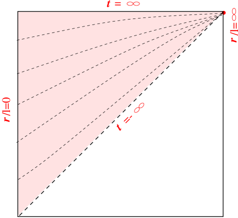
Figure 12: Penrose diagram of de Sitter spacetime in planar coordinates.

6 Discussion

In this review, we have discussed classical geometry of $d$-dimensional de Sitter spacetime in detail : Sections include introduction of four representative coordinates (global (or closed), conformal, planar (or inflationary), static), identification of Killing vectors, geodesic motions, cosmological implication, and Penrose diagrams.

Two important subjects are missing : One is group theoretic approach of the de Sitter spacetime and the other is energy because we do believe they have to be systematically dealt with quantum theoretic topics like supersymmetry and Hamiltonian formulation of quantum theory. Once we try to supersymmetrize de Sitter group, inconsistency is easily encountered, that either a supergroup including both unitary representations and isometries of the de Sitter spacetime is absent or any action compatible with de Sitter local supersymmetry contains vector ghosts [13]. In de Sitter spacetime two definitions are known to define the mass of it : One is the Abbott-Deser mass given as the eigenvalue of zeroth component of Virasoro generators and the other is the quasilocal mass obtained from Brown-York stress tensor associated to a boundary of a spacetime [14]. However, unitarity and conserved energy are not satisfied simultaneously in quantum theory in the de Sitter spacetime, and structure of de Sitter vacuum seems to ask more discussion [7, 5, 15].

Strikingly enough recent cosmological observations suggest the existence of extremely-small positive cosmological constant, however it just leads to a new form of terrible cosmological constant problem. In the present stage, it seems to force us to find its solution by understanding quantum gravity (in de Sitter spacetime). Obviously the topics we reviewed form a basis for the following research subjects still in progress, e.g., de Sitter entropy and thermodynamics, dS/CFT correspondence, trans-Planckian cosmology, understanding of vacuum energy in the context of string theory, and etc, of which ultimate goal should be perfect understanding of the cosmological constant problem as consequence of constructed quantum gravity.

Appendix A Various Quantities

For convenience, various formulas and quantities which have been used in the previous sections are summarized in the following four subsections.

A.1 Global (closed) coordinates

From the metric (3.21) of the global coordinates ($\tau,\theta_{i}$), nonvanishing components of covariant metric $g_{\mu\nu}$ are

$$g_{\tau\tau}=-1~{}~{}\mbox{and}~{}~{}g_{ii}=l^{2}f^{2}\prod_{j=1}^{i-1}\sin^{2}\theta_{j}\;,$$ (A.1)

and its inverse $g^{\mu\nu}$ has

$$g^{\tau\tau}=-1~{}~{}\mbox{and}~{}~{}g^{ii}=1/\left(l^{2}f^{2}\prod_{j=1}^{i-1}\sin^{2}\theta_{j}\right)\;.$$ (A.2)

Jacobian factor $g$ of the metric (A.1) becomes

$$g=-(l^{2}f^{2})^{d-1}\prod_{j=1}^{d-1}\prod_{i=1}^{j-1}\sin^{2}\theta_{i}\;.$$ (A.3)

Nonvanishing components of the connection $\Gamma^{\mu}_{\nu\rho}$ are

$$\displaystyle\Gamma^{i}_{\tau i}=\frac{1}{f}\left(\frac{df}{d\tau}\right)\;,~{}~{}~{}\Gamma^{\tau}_{ii}=l^{2}f\left(\frac{df}{d\tau}\right)\prod_{j=1}^{i-1}\sin^{2}\theta_{j}\;,$$

$$\displaystyle\Gamma^{i}_{jj}=-\sin\theta_{i}\cos\theta_{i}\prod_{j=i+1}^{j-1}\sin^{2}\theta_{j}\;,~{}~{}~{}\Gamma^{i}_{ij}=\frac{\cos\theta_{j}}{\sin\theta_{j}}\;.$$ (A.4)

For completeness, we mention non-zero components of the Riemann curvature tensor $R^{\mu}_{\;\nu\rho\sigma}$, which are consistent with Eq. (2.9) :

$$\displaystyle R^{\tau}_{\;i\tau i}=l^{2}f\left(\frac{d^{2}f}{d\tau^{2}}\right)\prod_{j=1}^{i-1}\sin^{2}\theta_{j}\;,~{}~{}~{}R^{i}_{\;\tau i\tau}=-\frac{1}{f}\left(\frac{d^{2}f}{d\tau^{2}}\right)\;,$$

$$\displaystyle R^{i}_{\;jij}=\left[1+l^{2}\left(\frac{df}{d\tau}\right)^{2}\right]\prod_{j=1}^{i-1}\sin^{2}\theta_{j}\;,$$ (A.5)

and the Ricci tensor $R_{\mu\nu}$ :

$$R_{\tau\tau} = -(d-1)\frac{1}{f}\left(\frac{d^{2}f}{d\tau^{2}}\right)\;,$$

$$R_{ii} = \left\{l^{2}f\left(\frac{d^{2}f}{d\tau^{2}}\right)+(d-2)\left[1+l^{2}\left(\frac{df}{d\tau}\right)^{2}\right]\right\}\prod_{j=1}^{i-1}\sin^{2}\theta_{j}\;.$$ (A.6)

Curvature scalar $R$ coincides with the formula in Eq. (3.22).

A.2 Conformal coordinates

From the metric (3.32) of the conformal coordinates ($T,\theta_{i}$), nonvanishing components of covariant metric $g_{\mu\nu}$ are

$$g_{TT}=-F^{2}~{}~{}\mbox{and}~{}~{}g_{ii}=l^{2}F^{2}\prod_{j=1}^{i-1}\sin^{2}\theta_{j}\;,$$ (A.7)

and its inverse $g^{\mu\nu}$ has

$$g^{TT}=-1/F^{2}~{}~{}\mbox{and}~{}~{}g^{ii}=1/\left(l^{2}F^{2}\prod_{j=1}^{i-1}\sin^{2}\theta_{j}\right)\;.$$ (A.8)

Jacobian factor $g$ of the metric (A.7) becomes

$$g=-\frac{(lF)^{2d}}{l^{2}}\prod_{j=1}^{d-1}\prod_{i=1}^{j-1}\sin^{2}\theta_{i}\;.$$ (A.9)

Nonvanishing components of the connection $\Gamma^{\mu}_{\nu\rho}$ are

$$\displaystyle\Gamma^{T}_{TT}=\Gamma^{i}_{Ti}=\frac{1}{F}\left(\frac{dF}{dT}\right)\;,~{}~{}~{}\Gamma^{T}_{ii}=\frac{l^{2}}{F}\left(\frac{dF}{dT}\right)\prod_{j=1}^{i-1}\sin^{2}\theta_{j}\;,$$

$$\displaystyle\Gamma^{i}_{jj}=-\sin\theta_{i}\cos\theta_{i}\prod_{j=i+1}^{j-1}\sin^{2}\theta_{j}\;,~{}~{}~{}\Gamma^{i}_{ij}=\frac{\cos\theta_{j}}{\sin\theta_{j}}\;.$$ (A.10)

Non-zero components of the Riemann curvature tensor $R^{\mu}_{\;\nu\rho\sigma}$ consistent with Eq. (2.9) are

$$R^{T}_{\;iTi} = \frac{l^{2}}{F^{2}}\left(F\frac{d^{2}F}{dT^{2}}-\frac{dF}{dT}\right)\prod_{j=1}^{i-1}\sin^{2}\theta_{j}\;,$$

$$R^{i}_{\;TiT} = -\frac{1}{F^{2}}\left[F\frac{d^{2}F}{dT^{2}}-\left(\frac{dF}{dT}\right)^{2}\right]\;,$$

$$R^{i}_{\;jij} = \frac{1}{F^{2}}\left[F^{2}+\left(\frac{dF}{dT}\right)^{2}\right]\prod_{j=1}^{i-1}\sin^{2}\theta_{j}\;,$$ (A.11)

and non-zero components of the Ricci tensor $R_{\mu\nu}$ are

$$R_{TT} = -(d-1)\frac{1}{F^{2}}\left[F\frac{d^{2}F}{dT^{2}}-\left(\frac{dF}{dT}\right)^{2}\right]\;,$$

$$R_{ii} = \frac{1}{l^{2}F^{2}}\left[F\left(\frac{d^{2}F}{dT^{2}}\right)+(d-3)\left(\frac{dF}{dT}\right)^{2}+(d-2)F^{2}\right]\prod_{j=1}^{i-1}\sin^{2}\theta_{j}\;.$$ (A.12)

Therefore, curvature scalar $R$ in the conformal coordinates coincides with the formula in Eq. (3.37).

A.3 Planar (inflationary) coordinates

From the metric (3.41) of the planar coordinates (${\sf t},x_{i}$), nonvanishing components of covariant metric $g_{\mu\nu}$ are

$$g_{\sf tt}=-1~{}~{}\mbox{and}~{}~{}g_{ij}=a(\sf t)^{2}\gamma_{ij}\;,$$ (A.13)

and its inverse $g^{\mu\nu}$ has

$$g^{\sf tt}=-1~{}~{}\mbox{and}~{}~{}g^{ij}=\gamma^{ij}a^{-2}\;,$$ (A.14)

where $\gamma^{ij}\gamma_{jk}=\delta^{i}_{k}$. Jacobian factor $g$ of the metric (A.13) becomes

$$g=-a^{2(d-1)}\gamma\;,$$ (A.15)

where $\gamma=det\gamma_{ij}$. Nonvanishing components of the connection $\Gamma^{\mu}_{\nu\rho}$ are

$$\Gamma^{\sf t}_{ij}=a\left(\frac{da}{d{\sf t}}\right)\gamma_{ij}\;,~{}~{}~{}\Gamma^{i}_{{\sf t}j}=\frac{1}{a}\left(\frac{da}{d{\sf t}}\right)\delta^{i}_{j}\;,~{}~{}~{}\Gamma^{i}_{jk}=\frac{\gamma^{il}}{2}(\partial_{j}\gamma_{lk}+\partial_{k}\gamma_{lj}-\partial_{l}\gamma_{jk})\;.$$ (A.16)

Non-zero components of the Riemann curvature tensor $R^{\mu}_{\;\nu\rho\sigma}$ consistent with Eq. (2.9) are

$$\displaystyle{R^{\sf t}_{\;i{\sf t}i}=a\left(\frac{d^{2}a}{d{\sf t}^{2}}\right)\;,~{}~{}~{}R^{i}_{\;{\sf t}i{\sf t}}=-\frac{1}{a}\left(\frac{d^{2}a}{d{\sf t}^{2}}\right)\;,}$$

$$\displaystyle{R^{i}_{\;jkl}=\left[\left(\frac{da}{d{\sf t}}\right)^{2}+k\right]\left(\delta^{i}_{k}\gamma_{jl}-\delta^{i}_{l}\gamma_{kj}\right)\;,~{}~{}~{}R^{\sf t}_{\;ijk}=a\left(\frac{da}{d{\sf t}}\right)\left[\partial_{j}\gamma_{ki}-\partial_{k}\gamma_{ji}+\partial_{i}\gamma_{jk}\right]\;,}$$ (A.17)

and non-zero components of the Ricci tensor $R_{\mu\nu}$ are

$$R_{\sf tt}=-\frac{d-1}{a}\left(\frac{d^{2}a}{d{\sf t}^{2}}\right)\;,~{}~{}~{}R_{ij}=\left[a\left(\frac{d^{2}a}{d{\sf t}^{2}}\right)+(d-2)\left(\frac{da}{d\sf t}\right)^{2}+(d-2)k\right]\gamma_{ij}\;.$$ (A.18)

Therefore, curvature scalar $R$ in the planar coordinates coincides with the formula in Eq. (3.49).

A.4 Static coordinates

From the metric (3.67) of the static coordinates ($t,r,\theta_{a}$), nonvanishing components of covariant metric $g_{\mu\nu}$ are

$$g_{tt}=-A(r)e^{2\Omega(r)}\;,~{}~{}~{}~{}~{}g_{rr}=\frac{1}{A(r)}\;,~{}~{}~{}~{}~{}g_{\theta_{a}\theta_{a}}=r^{2}\prod_{a=1}^{b-1}\sin^{2}\theta_{a}\;,$$ (A.19)

and its inverse $g^{\mu\nu}$ has

$$g^{tt}=-\frac{e^{-2\Omega}}{A}\;,~{}~{}~{}~{}~{}g^{rr}=A\;,~{}~{}~{}~{}~{}g^{\theta_{a}\theta_{a}}=1/\left(r^{2}\prod_{a=1}^{b-1}\sin^{2}\theta_{a}\right)\;.$$ (A.20)

Jacobian factor $g$ of the metric (A.19) becomes

$$g=-e^{2\Omega}r^{2(d-2)}\prod_{b=1}^{d-2}\prod_{a=1}^{b-1}\sin^{2}\theta_{a}\;.$$ (A.21)

Nonvanishing components of the connection $\Gamma^{\mu}_{\nu\rho}$ are

$$\displaystyle\Gamma^{t}_{rt}=\frac{1}{2A}\left(\frac{dA}{dr}+2A\frac{d\Omega}{dr}\right)\;,~{}~{}~{}\Gamma^{r}_{tt}=\frac{Ae^{2\Omega}}{2}\left(\frac{dA}{dr}+2A\frac{d\Omega}{dr}\right)\;,$$

$$\displaystyle\Gamma^{r}_{rr}=-\frac{1}{2A}\left(\frac{dA}{dr}\right)\;,~{}~{}~{}\Gamma^{\theta_{a}}_{r\theta_{a}}=\frac{1}{r}\;,~{}~{}~{}\Gamma^{\theta_{a}}_{\theta_{b}\theta_{a}}=\frac{\cos\theta_{b}}{\sin\theta_{b}}\;,$$

$$\displaystyle\Gamma^{r}_{\theta_{a}\theta_{a}}=-rA\prod_{a=1}^{a-1}\sin^{2}\theta_{a}\;,~{}~{}~{}\Gamma^{\theta_{a}}_{\theta_{b}\theta_{b}}=-\sin\theta_{a}\cos\theta_{a}\prod_{a=a+1}^{b-1}\sin^{2}\theta_{a}\;.$$ (A.22)

Non-zero components of the Riemann curvature tensor $R^{\mu}_{\;\nu\rho\sigma}$ consistent with Eq. (2.9) are

$$\displaystyle R^{r}_{\;trt}=\frac{Ae^{2\Omega}}{2}\left[3\left(\frac{dA}{dr}\right)\left(\frac{d\Omega}{dr}\right)+2A\left(\frac{d\Omega}{dr}\right)^{2}+\frac{d^{2}A}{dr^{2}}+2A\left(\frac{d^{2}\Omega}{d^{2}r}\right)\right]\;,$$

$$\displaystyle R^{t}_{\;rtr}=-\frac{1}{2A}\left[3\left(\frac{dA}{dr}\right)\left(\frac{d\Omega}{dr}\right)+2A\left(\frac{d\Omega}{dr}\right)^{2}+\frac{d^{2}A}{dr^{2}}+2A\left(\frac{d^{2}\Omega}{d^{2}r}\right)\right]\;,$$

$$\displaystyle R^{\theta_{a}}_{\;r\theta_{a}r}=-\frac{1}{2rA}\left(\frac{dA}{dr}\right)\;,~{}~{}~{}R^{t}_{\;\theta_{a}t\theta_{a}}=-\frac{r}{2}\left[\frac{dA}{dr}+2A\left(\frac{d\Omega}{dr}\right)\right]\prod_{a=1}^{a-1}\sin^{2}\theta_{a}\;,$$

$$\displaystyle R^{r}_{\;\theta_{a}r\theta_{a}}=-\frac{r}{2}\left(\frac{dA}{dr}\right)\prod_{a=1}^{a-1}\sin^{2}\theta_{a}\;,~{}~{}~{}R^{\theta_{b}}_{\;\theta_{a}\theta_{b}\theta_{a}}=(1-A)\prod_{a=1}^{a-1}\sin^{2}\theta_{a}\;,$$

$$\displaystyle R^{\theta_{a}}_{\;t\theta_{a}t}=\frac{Ae^{2\Omega}}{2r}\left[\frac{dA}{dr}+2A\left(\frac{d\Omega}{dr}\right)\right]\;.$$ (A.23)

Non-zero components of the Ricci tensor $R_{\mu\nu}$ are

$$\displaystyle R_{tt}=\frac{Ae^{2\Omega}}{2r}\left\{(d-2)\left[\frac{dA}{dr}+2A\left(\frac{d\Omega}{dr}\right)\right]+r\left[3\left(\frac{dA}{dr}\right)\left(\frac{d\Omega}{dr}\right)+2A\left(\frac{d\Omega}{dr}\right)^{2}+\frac{d^{2}A}{dr^{2}}+2A\left(\frac{d^{2}\Omega}{d^{2}r}\right)\right]\right\}\;,$$

$$\displaystyle R_{rr}=-\frac{1}{2Ar}\left\{(d-2)\left(\frac{dA}{dr}\right)+r\left[3\left(\frac{dA}{dr}\right)\left(\frac{d\Omega}{dr}\right)+2A\left(\frac{d\Omega}{dr}\right)^{2}+\frac{d^{2}A}{dr^{2}}+2A\left(\frac{d^{2}\Omega}{d^{2}r}\right)\right]\right\}\;,$$

$$R_{\theta_{a}\theta_{a}}=\frac{r^{2}}{d-2}\left\{\frac{d-2}{r^{d-2}}\frac{d}{dr}\left[r^{d-3}(1-A)\right]-A\frac{d-2}{r}\frac{d\Omega}{dr}\right\}\prod_{b=1}^{a-1}\sin^{2}\theta_{b}\;.$$ (A.24)

Therefore, curvature scalar $R$ in the static coordinates coincides with the formula in Eq. (3.68). Here we obtain also simple derivative terms for the Einstein equations

$$\frac{R_{tt}}{A^{2}e^{2\Omega}}+R_{rr}=\frac{d-2}{r}\frac{d\Omega}{dr}\;,$$ (A.25)

$$\frac{R_{tt}}{Ae^{2\Omega}}+AR_{rr}+\frac{(d-2)R_{\theta_{a}\theta_{a}}}{r^{2}\displaystyle{\prod_{b=1}^{a-1}\sin^{2}\theta_{b}}}=\frac{d-2}{r^{d-2}}\frac{d}{dr}\left[r^{d-3}(1-A)\right]\;.$$ (A.26)

References

-
[1]
A.G. Riess et al, Astron. J. 116, 1009 (1998),
astro-ph/9805201,
Observational evidence from supernovae for an accelerating universe
and a cosmological constant;
P.M. Garnavich et al, Astrophys. J. 509, 74 (1998), astro-ph/9806396, Supernova limits on the cosmic equation of state;
S. Perlmutter et al, Astrophys. J. 517, 565 (1999), astro-ph/9812133, Measurements of Omega and Lambda from 42 high-redshift supernovae. - [2] For a review, see S. Weinberg, Rev. Mod. Phys. 61, 1 (1989), The cosmological constant problem.
-
[3]
For reviews, see
E. Witten, Marina del Rey 2000, Sources and detection of dark matter
and dark energy in the universe, pp.27-36, hep-ph/0002297,
The cosmological constant from the viewpoint of string theory;
S.M. Carroll, Living Rev. Rel. 4, 1 (2001), astro-ph/0004075, The cosmological constant;
S. Weinberg, Marina del Rey 2000, Sources and detection of dark matter and dark energy in the universe, pp.18-26, astro-ph/0005265, The cosmological constant problem;
P.J.E. Peebles and B. Ratra, To appear in Rev. Mod. Phys., astro-ph/0207347, The cosmological constant and dark energy;
T. Padmanabhan, to appear in Phys. Rep., hep-th/0212290, Cosmological constant - the weight of the vacuum;
and references therein. -
[4]
J. Martin and R.H. Brandenberger, Phys. Rev. D63,
123501 (2001), hep-th/0005209, The trans-Planckian problem of
inflationary cosmology;
R.H. Brandenberger and J. Martin, Mod. Phys. Lett. A16, 999 (2001), astro-ph/0005432, The robustness of inflation to changes in superplanck scale;
J.C. Niemeyer, Phys. Rev. D63, 123502 (2001), astro-ph/0005533, Inflation with a Planck scale frequency cutoff;
For a review, see R.H. Brandenberger, to appear in the proceedings of 2002 International Symposium on Cosmology and Particle Astrophysics, hep-th/0210186, Trans-Planckian physics and inflationary cosmology. -
[5]
N. Kaloper, M. Kleban, A. Lawrence, S. Shenker, and L.
Susskind, JHEP 0211, 037 (2002), hep-th/0209231, Initial
conditions for inflation;
U.H. Danielsson, JHEP 0207, 040 (2002), hep-th/0205227, Inflation, holography, and the choice of vacuum in de Sitter space. -
[6]
A. Strominger, JHEP 0111, 034 (2002), hep-th/0106113,
The dS/CFT correspondence;
For a review, see R. Bousso, Rev. Mod. Phys. 74, 825 (2002), hep-th/0203101, The holographic principle. - [7] N.D. Birrell and P.C.W. Davies, Quantum fields in curved space, chapter 5, Cambridge University Press.
- [8] E.W. Kolb and M.S. Turner, The early universe, chapters 8 11, Addison-Wesley Publishing Company.
-
[9]
S.W. Hawking and G.F.R. Ellis, Section 5.2 of The large scale structure of space-time, Cambridge University Press;
C.W. Misner, K.S. Thorne, and J.A. Wheeler, Gravitation, chapter 27, W.H. Freeman and Company;
S. Weinberg, Gravitation and cosmology, chapter 16, John Wiley Sons. - [10] For lecture notes, see M. Spradlin, A. Strominger, and A. Volovich, hep-th/0110007, Les Houches lecture on de Sitter space.
- [11] A.D. Polyanin and V.F. Zaitsev, Handbook of exact solutions for ordinary differential equations, CRC press.
- [12] G.W. Gibbons and S.W. Hawking, Phys. Rev. D15, 2738 (1977), Cosmological event horizons, thermodynamics, and particle creation.
-
[13]
K. Pilch, P. van Nieuwenhuizen, and M.F. Sohnius,
Commun. Math. Phys. 98, 105 (1985),
De Sitter superalgebras and supergravity;
C.M. Hull, JHEP 9807, 021 (1998), hep-th/9806146, Timelike T-duality, de Sitter space, large gauge theories and topological field theory. -
[14]
L.F. Abbott and S. Deser, Nucl. Phys. B195, 76 (1982),
Stability of Gravity with a Cosmological Constant;
J.D. Brown and J.W. York, Phys. Rev. D47, 1407 (1993), gr-qc/9209012, Quasilocal energy and conserved charges derived from the gravitational action. - [15] A. Kaiser and A. Chodos, Phys. Rev. D53, 787 (1996), Symmetry breaking in the static coordinate system of de Sitter space-time.