Quantum corrections to the mass and central charge of solitons
in 1+1 dimensions

Abstract

We first discuss how the longstanding confusion in the literature concerning one-loop quantum corrections to 1+1 dimensional solitons has finally been resolved. Then we use ’t Hooft and Veltman’s dimensional regularization to compute the kink mass, and find that chiral domain wall fermions, induced by fermionic zero modes, lead to spontaneous parity violation and an anomalous contribution to the central charge such that the BPS bound becomes saturated. On the other hand, Siegel’s dimensional reduction shifts this anomaly to the counter terms in the renormalized current multiplet. The $\gamma\cdot j$ superconformal anomaly is located in an evanescent counter term, and imposing supersymmetry, this counter term induces the same anomalous contribution to the central charge. Next we discuss a new regularization scheme: local mode regularization. The local energy density computed in this scheme satisfies the BPS equality (it is equal to the local central charge density). In an appendix we give a very detailed account of the DHN method to compute soliton masses applied to the supersymmetric kink.

1 Introduction

Quantum corrections to solitons were of great interest in the 1970’s and 1980’s [1, 2, 3], and again in the last few years, due to the present activity in quantum field theories with dualities between extended objects and pointlike objects. Dashen, Hasslacher, and Neveu [1], in a 1974 article that has become a classic, computed the one-loop corrections to the mass of the bosonic kink in $\phi^{4}$ field theory and to the bosonic soliton in sine-Gordon theory. For the latter, there exist exact analytical methods associated with the complete integrability of the system, authenticating the perturbative calculation. Our work here uses general principles but focuses on the kink, for which exact results are not available. Dashen et al. put the object (classical background field corresponding to kink or to sine-Gordon soliton) in a box of length $L$ to discretize the continuous spectrum, and used mode number regularization (equal numbers of modes in the topological and trivial sectors, including the zero mode in this counting) for the ultraviolet divergences. They imposed periodic boundary conditions (PBC) on the meson field which describes the fluctuations around the trivial or topological vacuum solutions, and added a logarithmically divergent mass counter term whose finite part was fixed by requiring absence of tadpoles in the trivial background. They found for the one-loop correction to the kink mass

$$\Delta M^{(1)}=\sum\frac{1}{2}\hbar\omega_{n}-\sum\frac{1}{2}\hbar\omega_{n}^{(0)}+\delta M=-\hbar m\left(\frac{3}{2\pi}-\frac{\sqrt{3}}{12}\right)<0\ \ ,$$ (1)

where $m$ is the mass of the meson in the trivial background and $\delta M$ the counterterm induced by renormalizing $m$. This result remains unchallenged.

The supersymmetric (susy) case, as well as the general case including fermions, proved more difficult. The action reads

$${\cal L}=-\frac{1}{2}\left(\partial_{\mu}\varphi\right)^{2}-\frac{1}{2}\bar{\psi}\!\!\not\!\partial\psi-\frac{1}{2}U^{2}-c\frac{1}{2}\frac{dU}{d\phi}\bar{\psi}\psi\ \ ,$$ (2)

where $-\frac{1}{2}U^{2}=-\frac{\lambda}{4}(\varphi^{2}-\mu^{2}/\lambda)^{2}$, the meson mass is $m=\mu\sqrt{2}$, and $c=1$ for supersymmetry. Dashen et al. did not publish the fermionic corrections to the soliton mass, stating “The actual computation of [the contribution to] $M^{(1)}$ [due to fermions] can be carried out along the lines of the Appendix. As the result is rather complicated and not particularly illuminating we will not give it here” (page 4137 of [1]).

Several authors have since performed the calculation of $M^{(1)}$ for the susy kink, and found different answers. It became clear that the answers depended on the choice of boundary conditions (BC) for the fluctuation fields, more precisely on the BC for the fermions. Moreover, it also became clear that one obtained different answers if one used different regularization schemes. At present these issues are believed to be fully understood as follows.

Boundary conditions: Boundary conditions distort fields near the boundary. This distortion creates spurious boundary energy which should be subtracted from the total energy in order to obtain the true mass of the kink. There are several ways to avoid the spurious boundary energy

• one may first compute the energy density ${\mathcal{E}}(x)$ and then integrate over a region which contains the kink but stays away from the boundaries [4];

• one may average overs sets of BC such that in the average the boundary energy cancels [5]. One such set of BC for fermions which has been studied in detail consists of periodic BC ($\psi^{\pm}(-L/2)=\psi^{\pm}(L/2)$), antiperiodic BC ($\psi^{\pm}(-L/2)=-\psi^{\pm}(L/2)$), twisted periodic BC ($\psi^{\pm}(-L/2)=\psi^{\mp}(L/2)$), and twisted antiperiodic BC ($\psi^{\pm}(-L/2)=-\psi^{\mp}(L/2)$);

• one may choose a set of BC which have no boundary. By this cryptic statement we mean BC which put the system on a circle (more precisely a Möbius strip) such that the system becomes translationally invariant and one cannot identify a point where the boundary is present [6]. In principle such BC could still lead to delocalized (homogeneously spread out) boundary energy, but this does not occur [7]. By using the $Z_{2}$ symmetry $\varphi_{K}(-x)=-\varphi_{K}(x)$ of the kink background, one such set of BC has been identified to be the twisted (anti)periodic BC in the kink sector;

• one may first consider a background which contains both a kink ($\mathrm{K}$) and an antikink ($\overline{\mathrm{K}}$) with periodic BC, and then divide the answer for the mass of this compound ${\mathrm{K}}\overline{\mathrm{K}}$ system by 2 [8, 5]. (Putting a kink next to an antikink, there is a small cusp in the background where the kink is joined to the antikink, but for large distances the effect of this cusp can be neglected. One can also find an exact solution which is everywhere smooth and has periodic BC (a “sphaleron”) but this involves transcendental functions.) In fact, if one begins with periodic BC for the fermions in this ${\mathrm{K}}\overline{\mathrm{K}}$ system, one finds that the mode solutions have either twisted periodic or twisted antiperiodic BC in between.

Regularization schemes: Several well-known regularization schemes have been applied to the calculation of the quantum kink mass and the quantum central charge. To regulate the various sums over zero-point energies one has used: mode number cutoff, energy-momentum cutoff, heat-kernel techniques, $\zeta$-function techniques, ’t Hooft-Veltman’s dimensional regularization, Siegel’s dimensional regularization (“dimensional reduction”). To regulate Feynman graphs, one has used higher-space-derivative regularization with factors $(1-\partial_{x}^{2}/M^{2})$ (this regularization of the kinetic terms but not the interactions preserves susy, although it breaks Lorentz invariance) and again dimensional regularization. It has turned out that the reason some of these schemes give incorrect answers is that they were applied incorrectly: one naively applied the rules which had been developed for a trivial background to the kink background. After proper modification, these schemes all now yield the same answers. It is of some interest (and useful for avoiding errors in future calculations) to point out the required modifications of all these schemes. In the following, however, we concentrate on discussing in detail the two variants of dimensional regularization as well as a newly proposed method to study the local energy distribution of the quantum mass, local mode regularization [9, 10].

The ’t Hooft-Veltman dimensional regularization can be employed in a susy preserving manner by embedding the minimally susy kink in $1\leq d\leq 2$ spatial dimensions. This leads to new physics, namely spontaneous parity breaking and chiral domain wall fermions, which provide a new explanation [11] for the origin of the anomalous contribution [4] to the central charge of the susy kink. Siegel’s dimension reduction, on the other hand, where $d\leq 1$, obtains this anomaly from an evanescent counter term to the superconformal current, which gives rise to an anomalous nonconservation at the quantum level of the conformal version of the central-charge current [11].

2 Dimensional regularization and reduction

2.1 One-loop bosonic kink mass

Probably the most elegant regularization scheme to avoid the difficulties of mode regularization in a finite box and the possibility of boundary energy is dimensional regularization by embedding the 1+1 dimensional kink in $n=d+1$ dimensions as a domain wall.

As has been shown in Ref. [12], this reproduces correctly the one-loop quantum mass of the bosonic 1+1 dimensional kink, as well as the surface tension of the higher-dimensional kink domain walls [13].

By analytic continuation of the number of extra transverse dimensions ($d-1$) of a kink domain wall, no further regularization is needed. Denoting the momenta pertaining to the extra dimensions by $\ell$ and reserving $k$ for the momentum along the kink, i.e. perpendicular to the kink domain wall, the energy of the latter per transverse volume $L^{d-1}$ is obtained from summing/integrating zero-point energies according to

$${M^{(1)}\over L^{d-1}} = {m^{3}\over 3\lambda}+{1\over 2}\sum_{B}\int_{-\infty}^{\infty}{d^{d-1}\ell\over(2\pi)^{d-1}}\sqrt{\omega_{B}^{2}+\ell^{2}}$$ (3)

$$+{1\over 2}\int_{-\infty}^{\infty}{dk\,d^{d-1}\ell\over(2\pi)^{d}}\sqrt{k^{2}+\ell^{2}+m^{2}}\,\delta_{K}^{\prime}(k)+\delta M$$

where the discrete sum is over the normalizable states $B$ of the 1+1-dimensional kink with energy $\omega_{B}$, and the integral is over the continuum part of the spectrum.

The spectrum of fluctuations for the 1+1-dimensional kink is known exactly [14]. It consists of a zero-mode, a bound state with energy $\omega_{B}^{2}/m^{2}=3/4$, and scattering states in a reflectionless potential for which the phase shift $\delta_{K}(k)=-2\arctan(3mk/(m^{2}-2k^{2}))$ in the kink background provides the difference in the spectral density, $\delta^{\prime}_{K}(k)$, between kink and trivial vacuum.

In a “minimal” renormalization scheme where tadpoles cancel but $Z_{\lambda}=1$, one has

$$\delta M={3m\over 2\pi}d{\Gamma({-d\over 2})\over\Gamma(-\frac{1}{2})(4\pi)^{d-1\over 2}}\int_{0}^{\infty}dk(k^{2}+m^{2})^{d-2\over 2},$$ (4)

yielding (with $x\equiv k/m$)

$${M^{(1)}\over L^{d-1}} = {m^{3}\over 3\lambda}+{\Gamma({-d\over 2})\,m^{d}\over\Gamma(-\frac{1}{2})(4\pi)^{d-1\over 2}}\biggl{\{}\frac{1}{2}\left(3\over 4\right)^{d\over 2}$$ (5)

$$\qquad\quad+{3\over 4\pi}\int_{-\infty}^{\infty}dx(x^{2}+1)^{d-2\over 2}\left[{-1\over 4x^{2}+1}+(d-1)\right]\biggr{\}}.$$

Here the first term within the braces is the contribution from the bound state with nonzero energy, and the second is the result of combining the last two terms in (3).

In the limit $d\to 1$, which corresponds to the 1+1 dimensional kink, one obtains

$$M^{(1)}_{d=1}={m^{3}\over 3\lambda}+\left({m\over 4\sqrt{3}}-{3m\over 2\pi}\right),$$ (6)

reproducing the well-known DHN result [1]. It is interesting to note that it is the last term in (6) that would be missed in a sharp-cutoff calculation (see Ref. [15]) and that it now arises from the last term in the square brackets of (5).

Eq. (5) is also valid for $d\to 2$ where it gives the surface tension of a 2+1 dimensional kink domain wall; for higher dimensions one has to include also a renormalization of the coupling $\lambda$. All these results are in agreement with those obtained previously by other methods [13].

2.2 One-loop susy kink mass

Dimensional regularization is more delicate in susy theories. To preserve susy, one should normally consider Siegel’s dimensional regularization by dimensional reduction [16, 17]. However, it is also possible to preserve susy by embedding the susy kink in dimensions $\leq 2+1$.

Embedding the susy kink in 2+1 dimensions gives a domain wall centered about a one-dimensional string on which the fermion mass vanishes (since $U^{\prime}(\varphi_{K})\propto\varphi_{K}$ vanishes at the center of the kink). The total energy $M$ of the domain wall is infinite but the energy density $M/L$ is finite; as a result there is strictly speaking no zero mode in 2+1 dimensions associated with translational invariance. Indeed, the zero mode of the kink is only normalizable in 1+1 dimensions, but one can construct eigenfunctions in 2+1 dimensions which are products of zero modes in 1+1 dimensions and plane waves in the orthogonal direction(s) (along the domain wall).

The 2+1 dimensional case is different also with respect to the discrete symmetries of (2). In 2+1 dimensions, $\gamma^{5}=\gamma^{0}\gamma^{1}\gamma^{2}=\pm{\bf 1}$ corresponding to the two inequivalent choices available for $\gamma^{2}=\pm\tau^{1}$ (in odd space-time dimensions the Clifford algebra has two inequivalent irreducible representations). Therefore, the sign of the fermion mass (Yukawa) term can no longer be reversed by $\psi\to\gamma^{5}\psi$ and there is no longer the $Z_{2}$ symmetry $\varphi\to-\varphi,\psi\to\gamma^{5}\psi$.

What the 2+1 dimensional model does break spontaneously is instead parity, which corresponds to changing the sign of one of the spatial coordinates. The Lagrangian is invariant under $x^{m}\to-x^{m}$ for a given spatial index $m=1,2$ together with $\varphi\to-\varphi$ (which thus is a pseudoscalar) and $\psi\to\gamma^{m}\psi$. Each of the trivial vacua breaks these invariances spontaneously, whereas a kink background in the $x^{1}$-direction with $\varphi_{K}(-x^{1})=-\varphi_{K}(x^{1})$ is symmetric with respect to $x^{1}$-reflections, but breaks $x^{2}=y$ reflection invariance.

This is to be contrasted with the 1+1 dimensional case, where parity ($x^{1}\to-x^{1}$) can be represented either by $\psi\to\gamma^{0}\psi$ and a true scalar $\varphi\to\varphi$ or by $\psi\to\gamma^{1}\psi$ and a pseudoscalar $\varphi\to-\varphi$. The former leaves the trivial vacuum invariant, and the latter the ground state of the kink sector.

In what follows we shall consider the quantum corrections to both, the mass of the susy kink and the tension of the domain string, together. We again use a minimal renormalization scheme, where inclusion of the fermionic tadpole loop simply replaces the prefactor $3$ in (4) by $(3-2)$.

In a Majorana representation of the Dirac matrices in terms of the usual Pauli matrices $\tau^{k}$ with $\gamma^{0}=-i\tau^{2}$, $\gamma^{1}=\tau^{3}$, $\gamma^{2}=\tau^{1}$ (added for $d=2$), and $C=\tau^{2}$ so that $\psi={\psi^{+}\choose\psi^{-}}$ with real $\psi^{+}(x,t)$ and $\psi^{-}(x,t)$, the equations for the bosonic and fermionic normal modes with frequency $\omega$ and longitudinal momentum $\ell$ (nonzero only when $d=2$) in the kink background $\varphi=\varphi_{K}$ read

$$[-\partial_{x}^{2}+U^{\prime}{}^{2}+UU^{\prime\prime}]\eta=(\omega^{2}-\ell^{2})\eta,$$ (7)

$$(\partial_{x}+U^{\prime})\psi^{+}+i(\omega+\ell)\psi^{-}=0,$$ (8)

$$(\partial_{x}-U^{\prime})\psi^{-}+i(\omega-\ell)\psi^{+}=0.$$ (9)

Acting with $(\partial_{x}-U^{\prime})$ on (8) and eliminating $\psi^{-}$ as well as $\varphi^{\prime}=-U$ shows that $\psi^{+}$ satisfies the same equation as the bosonic fluctuation $\eta$. Compared to $\psi^{+}$, the component $\psi^{-}$ has a continuous spectrum whose modes differ by an additional phase shift $\theta=-2\arctan(m/k)$ when traversing the kink from $x_{1}=-\infty$ to $x_{1}=+\infty$, which is determined only by $U^{\prime}(\varphi_{K}(x_{1}=\pm\infty))=\pm m$. Correspondingly, the difference of the spectral densities of the $\psi^{+}$-fluctuations in the kink and in the trivial vacuum equals that of the $\eta$-fluctuations, whereas that of $\psi^{-}$-fluctuations is obtained by replacing $\delta^{\prime}_{K}\to\delta^{\prime}_{K}+\theta^{\prime}$.

In the sum over zero-point energies for the one-loop quantum mass of the kink (when $d=1$),

$$\tilde{M}=\tilde{M}_{cl.}+\frac{1}{2}\left(\sum\omega_{B}-\sum\omega_{B}^{\prime}\right)-\frac{1}{2}\left(\sum\omega_{F}-\sum\omega_{F}^{\prime}\right)+\delta\tilde{M}\;,$$ (10)

one thus finds that the bosonic contributions from the continuous spectrum are canceled by the fermionic contributions except for the additional contribution involving $\theta^{\prime}(k)$ in the spectral density of the $\psi^{-}$ modes.

The discrete bound states cancel exactly, apart from the subtlety that the fermionic zero mode should be counted as half a fermionic mode [5]. In strictly 1+1 dimensions, the zero modes do not contribute simply because they carry zero energy, and for $d>1$, where they become massless modes, they do not contribute in dimensional regularization.

In a cutoff regularization in $d=2$, as we shall further discuss below, they in fact do play a role. Remarkably, the half-counting of the fermionic zero mode for $d=1$ has an analog for $d=2$ where the bosonic and fermionic zero modes of the kink correspond to massless modes with energy $|\omega|=|\ell|$. From (8) and (9) one finds that the fermionic kink zero mode $\psi^{+}\propto\varphi_{K}^{\prime}$, $\psi^{-}=0$ is a solution only for $\omega=+\ell$. It therefore cancels only half of the contributions from the bosonic kink zero mode which for $d=2$ have $\omega=\pm\ell$. For $d=2$ one thus finds that the fermionic zero mode of the kink corresponds to a chiral (Majorana-Weyl) fermion on the domain wall (string) in 2+1 dimensions. [18, 19].

In dimensional regularization, however, the kink zero modes and their massless counterparts for $d>1$ can be dropped, and the energy density of the susy domain wall reads

$${\tilde{M}^{(1)}\over L^{d-1}}={m^{3}\over 3\lambda}-\frac{1}{4}\int{dk\,d^{d-1}\ell\over(2\pi)^{d}}\sqrt{k^{2}+\ell^{2}+m^{2}}\,\theta^{\prime}(k)+\delta\tilde{M},$$ (11)

where

$$\theta^{\prime}(k)={2m\over k^{2}+m^{2}}.$$ (12)

With $\delta\tilde{M}={1\over 3}\delta M$ the logarithmic divergence in the integral in (11) as $d\to 1$ gets cancelled. A naive cut-off regularization at $d=1$ would actually lead to a total cancellation of the $k$-integral with the counter term $\delta\tilde{M}$, giving a vanishing quantum correction in renormalization schemes with $\lambda=\lambda_{0}$. In dimensional regularization there is now however a mismatch for $d\not=1$ and a finite remainder in the limit $d\to 1$ proportional to $(d-1)\Gamma(-(d-1)/2)$. The final result reads [13]

$${\tilde{M}^{(1)}\over L^{d-1}}={m^{3}\over 3\lambda}-{m^{d}\over(4\pi)^{d+1\over 2}}{2\over d}\Gamma({3-d\over 2})\,.$$ (13)

In view of the discussion of the central charge below, it is instructive to write the above finite remainder that dimensional regularization leaves behind for $d\to 1$ in the form

$${\tilde{M}^{(1)}\over L^{d-1}}-{m^{3}\over 3\lambda}=-{1\over 4}\int{dk\,d^{d-1}\ell\over(2\pi)^{d}}{\ell^{2}\over\omega}\theta^{\prime}(k)$$ (14)

which is obtained by combining the integral in (11) with the integral representation of the counter term (1/3 of the r.h.s. of (4)). Evidently, the nonvanishing result is entirely due to the momenta in the extra $d-1$ dimensions of a kink domain wall.

In the literature, at least to our knowledge, only the case of a supersymmetric kink ($d=1$) has been considered and dimensional regularization reproduces the result obtained before by Refs. [8, 20, 6, 21, 4, 22].

However, a (larger) number of papers have missed the contribution $-m/(2\pi)$, mostly because of the (implicit) use of an inconsistent energy-cutoff scheme [23, 24, 25, 26] or have obtained different answers because of the use of boundary conditions that accumulate a finite amount of energy at the boundaries [27, 15]. The former result is however now generally accepted and, in the case of the super-sine-Gordon model (where the same issues arise with the same results) in agreement with S-matrix factorization [28].

A new result, which follows from (13) and which will play a role for the discussion of central charges in the next section, is the nonvanishing one-loop correction

$${\tilde{M}^{(1)}_{d=2}\over L}=-{m^{2}\over 8\pi}$$ (15)

for the surface tension of the minimally susy kink domain wall in 2+1 dimensions.

In Ref. [29] the correct susy kink mass has also been obtained by employing a smooth energy (momentum) cutoff, the necessity of which becomes apparent, as in the purely bosonic case, by considering the 2+1 dimensional domain wall. Using a naive cutoff for $d=2$ one finds quadratic divergences which cancel only upon inclusion of the zero modes (which become massless modes in 2+1 dimensions). As we have discussed above, unlike the other bound states, these do not cancel because the fermionic zero mode becomes a chiral fermion on the domain-string world-sheet and thus cancels only half of the bosonic zero (massless) mode contribution, yielding

$$\int_{0}^{\infty}{d\ell\over 2\pi}\biggl{\{}\frac{1}{2}\sqrt{\ell^{2}}-\int_{-\Lambda_{k}}^{\Lambda_{k}}{dk\over 2\pi}\left[\sqrt{k^{2}+\ell^{2}+m^{2}}{m\over k^{2}+m^{2}}-{1\over\sqrt{k^{2}+\ell^{2}+m^{2}}}\right]\biggr{\}}$$

$$\stackrel{{\scriptstyle\Lambda_{k}\to\infty}}{{\longrightarrow}}\int_{0}^{\infty}{d\ell\over 2\pi}\biggl{\{}{\ell\over 2}-{\ell\over\pi}\arctan{\ell\over m}\biggr{\}}\sim\int_{0}^{\infty}{d\ell\over\pi}{m\over 2\pi}$$ (16)

which is however still linearly divergent. Smoothing out the cutoff in the $k$-integral does pick an additional (and for $d=1$ the only) contribution $-m/(2\pi)$, which is now necessary to have a finite result for $d=2$. This finite result then reads

$${\tilde{M}^{(1)}_{d=2}\over L}=-{1\over\pi}\int_{0}^{\infty}{d\ell\over 2\pi}\left(m-\ell\arctan{m\over\ell}\right)=-{m^{2}\over 8\pi}$$ (17)

in agreement with the result obtained above in dimensional regularization.

2.3 Susy algebra and its quantum corrections

2.3.1 Dimensional regularization

The susy algebra for the 1+1 and the 2+1 dimensional cases can both be covered by starting from 2+1 dimensions, the 1+1 dimensional case following from reduction by one spatial dimension.

In 2+1 dimensions one obtains classically [30]

$$\{Q^{\alpha},\bar{Q}_{\beta}\} = 2i(\gamma^{M})^{\alpha}{}_{\beta}P_{M}\ ,\quad(M=0,1,2)$$ (18)

$$= 2i(\gamma^{0}H+\gamma^{1}(\tilde{P}_{x}+\tilde{Z_{y}})+\gamma^{2}(\tilde{P}_{y}-\tilde{Z}_{x}))^{\alpha}{}_{\beta},$$

where we separated off two surface terms $\tilde{Z}_{m}$ in defining

$$\tilde{P}_{m}=\int d^{d}x\tilde{\mathcal{P}}_{m},\quad \tilde{\mathcal{P}}_{m}=\dot{\varphi}\,\partial_{m}\varphi-\frac{1}{2}(\bar{\psi}\gamma^{0}\partial_{m}\psi),$$ (19)

$$\tilde{Z}_{m}=\int d^{d}x\tilde{\mathcal{Z}}_{m},\quad \tilde{\mathcal{Z}}_{m}=U(\varphi)\partial_{m}\varphi=\partial_{m}W(\varphi)$$ (20)

with $W(\varphi)\equiv\int d\varphi\,U(\varphi)$.

Having a kink profile in the $x$-direction, which satisfies the Bogomolnyi equation $\partial_{x}\varphi_{K}=-U(\varphi_{K})$, one finds that with our choice of Dirac matrices

$$Q^{\pm}=\int d^{2}x[(\dot{\varphi}\mp\partial_{y}\varphi)\psi^{\pm}+(\partial_{x}\varphi\pm U(\varphi))\psi^{\mp}],$$ (21)

$$\{Q^{\pm},Q^{\pm}\}=2(H\pm(\tilde{Z}_{x}-\tilde{P}_{y})),$$ (22)

and the charge $Q^{+}$ leaves the topological (domain-wall) vacuum $\varphi=\varphi_{K}$, $\psi=0$ invariant. This corresponds to classical BPS saturation, since with $P_{x}=0$ and $\tilde{P}_{y}=0$ one has $\{Q^{+},Q^{+}\}=2(H+\tilde{Z}_{x})$ and, indeed, with a kink domain wall $\tilde{Z}_{x}/L^{d-1}=W(+v)-W(-v)=-M/L^{d-1}$.

At the quantum level, hermiticity of $Q^{\pm}$ implies

$$\langle s|H|s\rangle\geq|\langle s|P_{y}|s\rangle|\equiv|\langle s|(\tilde{P}_{y}-\tilde{Z}_{x})|s\rangle|.$$ (23)

This inequality is saturated when

$$Q^{+}|s\rangle=0$$ (24)

so that BPS states correspond to massless states $P_{M}P^{M}=0$ with $P_{y}=M$ for a kink domain wall in the $x$-direction [31], however with infinite momentum and energy unless the $y$-direction is compact with finite length $L$. An antikink domain wall has instead $Q^{-}|s\rangle=0$. In both cases, half of the supersymmetry is spontaneously broken.

Classically, the susy algebra in 1+1 dimensions is obtained from (18) simply by dropping $\tilde{P}_{y}$ as well as $\tilde{Z}_{y}$ so that $P_{x}\equiv\tilde{P}_{x}$. The term $\gamma^{2}\tilde{Z}_{x}$ remains, however, with $\gamma^{2}$ being the nontrivial $\gamma^{5}$ of 1+1 dimensions. The susy algebra simplifies to

$$\{Q^{\pm},Q^{\pm}\}=2(H\pm Z),\quad\{Q^{+},Q^{-}\}=2P_{x}$$ (25)

and one has the inequality

$$\langle s|H|s\rangle\geq|\langle s|Z|s\rangle|$$ (26)

for any quantum state $s$. BPS saturated states have $Q^{+}|s\rangle=0$ or $Q^{-}|s\rangle=0$, corresponding to kink and antikink, respectively, and break half of the supersymmetry.

In a kink (domain wall) background with only nontrivial $x$ dependence, the central charge density $\tilde{\mathcal{Z}}_{x}$ receives nontrivial contributions. Expanding $\tilde{\mathcal{Z}}_{x}$ around the kink background gives

$$\tilde{\mathcal{Z}}_{x}=U\partial_{x}\varphi_{K}-\frac{\delta\mu^{2}}{\sqrt{2\lambda}}\partial_{x}\varphi_{K}+\partial_{x}(U\eta)+\frac{1}{2}\partial_{x}(U{{}^{\prime}}\eta^{2})+O(\eta^{3}).$$ (27)

where only the part quadratic in the fluctuations contributes to the integrated quantity at one-loop order. However, this matches precisely the counter term $\delta M$ from requiring vanishing tadpoles. Straightforward application of the rules of dimensional regularization thus leads to a null result for the net one-loop correction to $\langle\tilde{Z}_{x}\rangle$ in the same way as found in Refs. [24, 25, 15, 6] in other schemes.

On the other hand, by considering the less singular combination $\langle H+\tilde{Z}_{x}\rangle$ and showing that it vanishes exactly, it was concluded in Ref. [21] that $\langle\tilde{Z}_{x}\rangle$ has to compensate any nontrivial result for $\langle H\rangle$, which in Ref. [21] was obtained by subtracting successive Born approximations for scattering phase shifts. In fact, Ref. [21] explicitly demonstrates how to rewrite $\langle\tilde{Z}_{x}\rangle$ into $-\langle H\rangle$, apparently without the need for the anomalous terms in the quantum central charge operator postulated in Ref. [4].

The resolution of this discrepancy is that Ref. [21] did not regularize $\langle\tilde{Z}_{x}\rangle$ and therefore the manipulations needed to rewrite it as $-\langle H\rangle$ (which eventually is regularized and renormalized) are ill-defined. Using dimensional regularization naively one in fact obtains a nonzero result for $\langle H+\tilde{Z}_{x}\rangle$, apparently in violation of susy.

However, dimensional regularization by embedding the kink as a domain wall in (up to) one higher dimension, which preserves susy, instead leads to

$$\langle H+\tilde{Z}_{x}-\tilde{P}_{y}\rangle=0,$$ (28)

i.e. the saturation of (23), as we shall now verify.

The bosonic contribution to $\langle\tilde{P}_{y}\rangle$ involves

$$\frac{1}{2}\langle\dot{\eta}\partial_{y}\eta+\partial_{y}\eta\dot{\eta}\rangle=-\int\frac{d^{d-1}\ell}{(2\pi)^{d-1}}\sum\!\!\!\!\!\!\!\int{dk\over 2\pi}\ \frac{\ell}{2}|\phi_{k}(x)|^{2},$$ (29)

where the $\phi_{k}(x)$ are the mode functions of the fluctuation field operator $\eta$. The $\ell$-integral factorizes and gives zero both because it is a scale-less integral and because the integrand is odd in $\ell$.

The fermions on the other hand turn out to give nontrivial contributions: The mode expansion for the fermionic field operator reads

$$\psi\! = \!\psi_{0}+\int\frac{d^{d-1}\ell}{(2\pi)^{\frac{d-1}{2}}}\sum\!\!\!\!\!\!\!\int^{\prime}\frac{dk}{\sqrt{4\pi\omega}}\left[b_{k,\ell}\ e^{-i(\omega t-\ell y)}{{\scriptstyle\sqrt{\omega+\ell}}\ \phi_{k}(x)\choose{\scriptstyle\sqrt{\omega-\ell}}\ is_{k}(x)}+b^{\dagger}_{k,\ell}\ (c.c.)\right],$$ (30)

$$\psi_{0}=\int\frac{d^{d-1}\ell}{(2\pi)^{\frac{d-1}{2}}}b_{0,\ell}\ e^{-i\ell(t-y)}{\phi_{0}\choose 0},\quad b^{\dagger}_{0}(\ell)=b_{0}(-\ell),$$

where $\psi_{0}$ is the fermionic zero-mode lifted to a Majorana-Weyl domain wall fermion, and $s_{k}=\frac{1}{\sqrt{\omega^{2}-\ell^{2}}}(\partial_{x}+U{{}^{\prime}})\phi_{k}$. This leads to

$$\langle\tilde{\mathcal{P}}_{y}\rangle = \frac{i}{2}\langle\psi^{\dagger}\partial_{y}\psi\rangle$$ (31)

$$= \frac{1}{2}\int\frac{d^{d-1}\ell}{(2\pi)^{d-1}}\sum\!\!\!\!\!\!\!\int{dk\over 2\pi}{\ell\over 2\omega}\left[(\omega+\ell)|\phi_{k}|^{2}+(\omega-\ell)|s_{k}|^{2}\right]$$

$$= \frac{1}{2}\int\frac{d^{d-1}\ell}{(2\pi)^{d-1}}\ \ell\ \theta(-\ell)\ |\phi_{0}|^{2}+$$

$$+\frac{1}{2}\int\frac{d^{d-1}\ell}{(2\pi)^{d-1}}\sum\!\!\!\!\!\!\!\int^{\prime}{dk\over 2\pi}\left(\frac{\ell}{2}(|\phi_{k}|^{2}+|s_{k}|^{2})+\frac{\ell^{2}}{2\omega}(|\phi_{k}|^{2}-|s_{k}|^{2})\right).\qquad$$

From the last sum-integral we have separated off the contribution of the zero mode of the kink (the chiral domain wall fermion for $d>1$). The contribution of the latter no longer vanishes by symmetry, but the $\ell$-integral is still scale-less and therefore put to zero in dimensional regularization. The first sum-integral on the right-hand side is again zero by both symmetry and scalelessness, but the final term is not: The $\ell$-integration no longer factorizes because $\omega=\sqrt{k^{2}+\ell^{2}+m^{2}}$, and leads to a nonvanishing result, which, as one can show [11], is identical to the finite net contribution in $\langle\mathcal{H}\rangle$. For the integrated quantities, this equality can be seen by comparing with (14) upon using that $\int dx(|\phi_{k}|^{2}-|s_{k}|^{2})=\theta^{\prime}(k)$.

So for all $d\leq 2$ we have BPS saturation, $\langle H\rangle=|\langle\tilde{Z}_{x}-\tilde{P}_{y}\rangle|$, which in the limit $d\to 1$, the susy kink, is made possible by a nonvanishing $\langle\tilde{P}_{y}\rangle$. The anomaly in the central charge is seen to arise from a parity-violating contribution in $d=1+\epsilon$ dimensions which is the price to be paid for preserving (minimal) supersymmetry when going up in dimensions to embed the susy kink as a domain wall.

To summarize, in 2+1 dimensions, we have $P_{y}=\tilde{P}_{y}-\tilde{Z}_{x}$ and $|\langle P_{y}\rangle|=\langle H\rangle$, where $\tilde{P}$ and $\tilde{Z}$ were defined in (18). Classically, this BPS saturation is guaranteed by $\tilde{Z}_{x}$ alone. At the quantum level, however, the quantum corrections to the latter are cancelled completely by the counter term from renormalizing tadpoles to zero. All nontrivial corrections come from the “genuine” momentum operator $\tilde{P}_{y}$, and are due to having a spontaneous breaking of parity.

In the limit of 1+1 dimensions, because $\gamma^{2}|_{D=2+1}=\gamma^{5}|_{D=1+1}$, one has to make the identification $Z=\tilde{Z}_{x}-\tilde{P}_{y}$. For $\tilde{Z}_{x}$, one again does not obtain net quantum corrections. However, the expectation value $\langle\tilde{P}_{y}\rangle$ does not vanish in the limit $d\to 1$, although there is no longer an extra dimension. The spontaneous parity violation in the 2+1 dimensional theory, which had to be considered in order to preserve susy, leaves a finite imprint upon dimensional reduction to 1+1 dimensions by providing an anomalous additional contribution to $\langle\tilde{Z}_{x}\rangle$ balancing the nontrivial quantum correction $\langle H\rangle$.

2.3.2 Dimensional reduction

We now show how the central charge anomaly can be recovered from Siegel’s version of dimensional regularization [16, 17] where $n$ is smaller than the dimension of spacetime and where one keeps the number of field components fixed, but lowers the number of coordinates and momenta from 2 to $n<2$. At the one-loop level one encounters 2-dimensional $\delta_{\mu}^{\nu}$ coming from Dirac matrices, and $n$-dimensional $\hat{\delta}_{\mu}^{\nu}$ from loop momenta. An important concept which is going to play a role is that of the evanescent counterterms [32] involving the factor ${1\over\epsilon}\hat{\hat{\delta}}{}_{\mu}^{\nu}$, where $\hat{\hat{\delta}}{}_{\mu}^{\nu}\equiv\delta_{\mu}^{\nu}-\hat{\delta}_{\mu}^{\nu}$ has only $\epsilon=2-n$ nonvanishing components.

Consider now the supercurrent $j_{\mu}=-(\not\!\partial\varphi+U(\varphi))\gamma_{\mu}\psi$. In the trivial vacuum, expanding into quantum fields yields

$$j_{\mu}=-\left(\not\!\partial\eta+U^{\prime}(v)\,\eta+\frac{1}{2}U^{\prime\prime}(v)\,\eta^{2}\right)\gamma_{\mu}\psi+{1\over\sqrt{2\lambda}}\delta\mu^{2}\gamma_{\mu}\psi,$$ (32)

where $v=\mu/\sqrt{\lambda}$. Only matrix elements with one external fermion are divergent. The term involving $U^{\prime\prime}(v)\eta^{2}$ in (32) gives rise to a divergent scalar tadpole that is cancelled completely by the counter term $\delta\mu^{2}$ (which itself is due to an $\eta$ and a $\psi$ loop). The only other divergent diagram is due to the term involving $\not\!\partial\eta$ in (32) and has the form of a $\psi$-selfenergy. Its singular part reads

$$\langle 0|j_{\mu}|p\rangle^{\rm div}=iU^{\prime\prime}(v)\int_{0}^{1}dx\int{d^{n}\kappa\over(2\pi)^{n}}{\not\!\kappa\gamma_{\mu}\!\not\!\kappa\over[\kappa^{2}+p^{2}x(1-x)+m^{2}]^{2}}u(p).$$ (33)

Using $\hat{\delta}_{\mu}^{\nu}\equiv\delta_{\mu}^{\nu}-\hat{\hat{\delta}}{}_{\mu}^{\nu}$ we find that under the integral

$$\not\!\kappa\gamma_{\mu}\!\!\not\!\kappa=-\kappa^{2}(\delta_{\mu}^{\lambda}-{2\over n}\hat{\delta}_{\mu}^{\lambda})\gamma_{\lambda}={\epsilon\over n}\kappa^{2}\gamma_{\mu}-{2\over n}\kappa^{2}\hat{\hat{\delta}}{}_{\mu}^{\lambda}\gamma_{\lambda}$$

so that

$$\langle 0|j_{\mu}|p\rangle^{\rm div}={U^{\prime\prime}(v)\over 2\pi}{\hat{\hat{\delta}}{}_{\mu}^{\lambda}\over\epsilon}\gamma_{\lambda}u(p).$$ (34)

Hence, the regularized one-loop contribution to the susy current contains the evanescent operator

$$j_{\mu}^{\rm div}={U^{\prime\prime}(\varphi)\over 2\pi}{\hat{\hat{\delta}}{}_{\mu}^{\lambda}\over\epsilon}\gamma_{\lambda}\psi.$$ (35)

This is by itself a conserved quantity, because all fields depend only on the $n$-dimensional coordinates. The renormalized susy current $j_{\mu}^{\rm ren.}=j_{\mu}-j_{\mu}^{div}$ is thus still conserved, but from the evanescent counter term it receives a nonvanishing contribution to $\gamma\cdot j^{\rm ren.}$ which appears in the divergence of the renormalized conformal-susy current $j_{\mu}^{\rm ren.}$

$$\partial^{\mu}(\not\!xj_{\mu}^{\rm ren.})_{\rm anom.}=-\gamma^{\mu}j_{\mu}^{\rm div}=-{U^{\prime\prime}\over 2\pi}\psi.$$ (36)

(There are also nonvanishing nonanomalous contributions to $\partial^{\mu}(\mbox{$\not\!x$}j_{\mu})$ because our model is not conformal-susy invariant at the classical level.)

Ordinary susy on the other hand is unbroken; there is no anomaly in the divergence of $j_{\mu}^{\rm ren.}$. A susy variation of $j_{\mu}$ involves the energy-momentum tensor and the topological central-charge current $\zeta_{\mu}$ according to

$$\delta j_{\mu}=-2T_{\mu}{}^{\nu}\gamma_{\nu}\epsilon-2\zeta_{\mu}\gamma^{5}\epsilon,$$ (37)

where classically $\zeta_{\mu}=\epsilon_{\mu\nu}U\partial^{\nu}\varphi$.

At the quantum level, the counter-term $j_{\mu}^{\rm ct}=-j_{\mu}^{\rm div}$ induces an additional contribution to the central charge current

$$\zeta_{\mu}^{\rm anom}={1\over 4\pi}{\hat{\hat{\delta}}{}_{\mu}^{\nu}\over\epsilon}\epsilon_{\nu\rho}\partial^{\rho}U^{\prime}$$ (38)

which despite appearances is a finite quantity: using that total antisymmetrization of the three lower indices has to vanish in two dimensions gives

$$\hat{\hat{\delta}}{}_{\mu}^{\nu}\epsilon_{\nu\rho}=\epsilon\epsilon_{\mu\rho}+\hat{\hat{\delta}}{}_{\rho}^{\nu}\epsilon_{\nu\mu}$$ (39)

and together with the fact the $U^{\prime}$ only depends on $n$-dimensional coordinates this finally yields

$$\zeta_{\mu}^{\rm anom}={1\over 4\pi}\epsilon_{\mu\rho}\partial^{\rho}U^{\prime}$$ (40)

in agreement with the anomaly in the central charge as obtained previously.

We emphasize that $\zeta_{\mu}$ itself does not require the subtraction of an evanescent counterterm. The latter only appears in the susy current $j_{\mu}$, which gives rise to a conformal-susy anomaly in $\not\!xj_{\mu}$. A susy variation of the latter shows that it forms a conformal current multiplet involving besides the dilatation current $T_{\mu\nu}x^{\nu}$ and the Lorentz current $T_{\mu}{}^{\nu}x^{\rho}\epsilon_{\nu\rho}$ also a current

$$j_{(\nu)}^{(\zeta)\mu}=x^{\rho}\epsilon_{\rho\nu}\zeta^{\mu}.$$ (41)

We identify this with the conformal central-charge current, which is to be distinguished from the ordinary central-charge current $\zeta_{\mu}$.

The anomalous contribution to the ordinary central charge is thus understood as the additional nonconservation at the quantum level of the conformal central-charge current (41). (Additional, because the model is not conformally invariant so that there is already nonconservation at the classical level.) This finally answers the question: what kind of anomaly corresponds to the anomalous contribution to the central charge?

3 Local Casimir energy for solitons

We have seen in the introduction that there is a problem with the regularization of the zero-point energies by means of mode number cutoff (equal numbers of modes in each sector, with careful counting of zero modes): it includes spurious boundary energy. On the other hand, the principle of mode regularization seems natural, so the question arises whether we can devise a mode number cutoff scheme without the unwanted boundary energy. This almost automatically leads to a new regularization scheme for Casimir sums, called local mode regularization. Given that each mode determines a mode function $\phi_{n}(x,t)$ (or $\psi_{n}(x,t)$ for the fermions) normalized such that for a large box with volume $L$ the $\phi_{n}(x,t)$ become at large $|x|$ a plane wave with unit strength (the corrections to these plane waves are of order $L^{-1/2}$), we can introduce a concept of local mode density $\rho(x)$ in the kink sector (and $\rho^{(0)}(x)$ in the trivial sector) as follows: $\rho(x)=\sum\phi_{n}^{\ast}(x)\phi_{n}(x)$. To regulate such sums we would like to again cut off the sum over $n$ at a large number $N$.

The kink mass contains the difference of the energy sum $\sum|\phi_{n}(x)|^{2}{\textstyle\frac{1}{2}}\omega_{n}$ in the kink sector and the energy sum $\sum|\phi_{n}^{(0)}(x)|^{2}{\textstyle\frac{1}{2}}\omega_{n}^{(0)}$ in the trivial sector. The problem is thus how to relate the regularization in one sector to that in the other sector. The most straightforward method would be to include the same number of terms in each sum, just as in the case of global mode number regularization. However in this way the sums would only indirectly take the presence of the kink into account (through the inequality of the $\omega_{n}$ and $\omega_{n}^{(0)}$).

We now formulate a principle which we have not yet been able to prove that it is equivalent to other principles, or that it preserves supersymmetry, but which gives correct answers for the kink mass and supersymmetric kink mass, and which is so simple that it deserves further study. Namely we require that the regulated mode densities in both sectors are equal. The function $\sum_{n=0}^{N}\phi_{n}^{\ast}(x)\phi_{n}(x)$ is a function of $N$ or equivalently of $\Lambda=2\pi N/L$, but for large $L$ we can interpolate it to become a function of a continuous variable $\Lambda$. Similarly, $\rho_{N}^{(0)}$ becomes a continuous function of $\Lambda$. Since $L^{-1}\int|\phi_{k}|^{2}dx=1$ counts each mode once, it may seem natural to also use $|\phi_{k}(x)|^{2}$ to count modes locally. However note that $\left<\varphi(x)\varphi(x)\right>$ contains $\sum|\phi_{k}(x)|^{2}\frac{1}{2\omega_{k}}$ while the energy density contains $\sum|\phi_{k}(x)|^{2}{\textstyle\frac{1}{2}}{\omega_{k}}$. The choice to use $\sum|\phi_{k}(x)|^{2}$ to define a regularization is perhaps natural, certainly more natural than for example $\sum|\phi_{k}(x)|^{4}$, but we have not proven that $\sum|\phi_{k}(x)|^{2}$ is the correct object.

If the density $\rho(x)$ is cut off at a large $\Lambda$, the density $\rho^{(0)}(x)$ should be cut off at a $\Lambda+\Delta\Lambda\equiv 2\pi N^{(0)}$ such that $\rho_{\Lambda}(x)$ is equal to $\rho^{(0)}_{\Lambda+\Delta\Lambda}(x)$. Far away from the kink all modes are plane waves, so for large $|x|$ one expects $\Delta\Lambda$ to vanish, but near the kink $\Delta\Lambda$ will be nonvanishing. This implies that $\Delta\Lambda$ is $x$-dependent, and the principle of local mode regularization takes the following form

$$\rho_{\Lambda}(x)=\rho^{(0)}_{\Lambda+\Delta\Lambda(x)}(x).$$ (42)

The regulated energy densities in the kink and the trivial sector, given by $\epsilon=\sum|\phi_{n}(x)|^{2}{\textstyle\frac{1}{2}}\omega_{n}$ and $\epsilon^{(0)}=\sum|\phi_{n}^{(0)}(x)|^{2}{\textstyle\frac{1}{2}}\omega_{n}^{(0)}$, will then in general be different if the regulated densities $\rho(x)$ and $\rho^{(0)}(x)$ are equal.

It is now straightforward to calculate the local Casimir mass of a soliton. It is given by

$$\epsilon_{\rm Cas}(x)=\epsilon(x)-\epsilon^{(0)}(x)=$$

$$\frac{1}{2}\omega_{B}\phi_{B}^{2}(x)+2\int_{0}^{\Lambda}\frac{dk}{2\pi}|\phi(k,x)|^{2}\frac{1}{2}\omega-2\int_{0}^{\Lambda+\Delta\Lambda(x)}\frac{dk}{2\pi}\frac{1}{2}\omega+\delta M(x).$$ (43)

The bound state yields a zero-point energy ${\textstyle\frac{1}{2}}\omega_{B}$ and has (normalizable) mode function $\phi_{B}(x)$, while the continuous spectrum in the kink sector consists of plane waves $\phi^{(0)}(k,x)=\exp{ikx}$. We rewrite this expression such that it is manifestly finite

$$\epsilon_{\rm Cas}(x)={\textstyle\frac{1}{2}}\omega_{B}\phi_{B}^{2}(x)$$

$$+\left\{2\int_{0}^{\Lambda}\frac{dk}{2\pi}\left(|\phi(x,k)|^{2}-1\right){\textstyle\frac{1}{2}}\omega+\delta M(x)\right\}-\frac{\Delta\Lambda(x)}{2\pi}\Lambda.$$ (44)

The last term is the ”anomaly”, it appears here as a term of the form $\Lambda/\Lambda$ because $\Delta\Lambda(x)$ is proportional to $1/\Lambda$ as well see presently.

In the kink sector $\phi(k,x)$ can be given explicitly. From the explicit form one finds that it can be expressed in terms of the wave functions of the discrete spectrum as follows

$$|\phi(k,x)|^{2}-1=-\sum_{j}\phi_{j}^{2}(x)\frac{2\sqrt{m^{2}-\omega_{j}^{2}}}{\omega^{2}-\omega^{2}_{j}}.$$ (45)

(For the kink $j$ refers to the zero mode with $\omega^{2}_{j}=0$ and the bound state with $\omega_{j}^{2}=3/4m^{2}$.) This formula seems to be new and we interpret it as a local version of the completeness relation. Integration over $k$ yields the usual completeness relation

$$\int_{-\infty}^{\infty}\frac{dk}{2\pi}\left\{|\phi(k,x)|^{2}-1\right\}+\phi_{0}^{2}(x)+\phi_{B}^{2}(x)=0,$$ (46)

but the local version allows us to evaluate $\Delta\Lambda$ as

$$\Delta\Lambda(x) = \int_{\Lambda}^{\infty}dk\,\left(1-|\phi(k,x)|^{2}\right)=2\int_{\Lambda}^{\infty}\!\!dk\,\sum_{j}{\sqrt{m^{2}-\omega_{j}^{2}}\over\omega^{2}-\omega_{j}^{2}}\phi_{j}^{2}(x)$$ (47)

$$= {3m^{2}\over 4\Lambda\cosh{mx\over 2}}+\mathcal{O}(\Lambda^{-2}).$$

The local counter term $\delta M(x)$ is of course equal to the term proportional to $\delta\mu^{2}$ in the energy density. We can now substitute all these relations and find then

$$\epsilon_{\rm Cas}(x)=\left(\frac{1}{2}\omega_{B}-\frac{m}{2\sqrt{3}}-\frac{m}{2\pi}\right)\phi_{B}^{2}(x)-\frac{m}{\pi}\phi_{0}^{2}(x).$$ (48)

We can rewrite this formula as

$$\epsilon_{\rm Cas}(x)=\sum_{j}\frac{1}{2}\left(1-\frac{2}{\pi}\arctan\frac{\omega_{j}}{\sqrt{m^{2}-\omega_{j}^{2}}}\right)\omega_{j}\phi^{2}_{j}(x)-\sum_{j}\frac{1}{\pi}\sqrt{m^{2}-\omega^{2}_{j}}\phi_{j}^{2}(x).$$ (49)

Such expressions are known for the total energy, but this local version seems new.

The local Casimir energy is not, however, equal to the local energy density. There are two further terms:

(i) the energy density contains a term ${\textstyle\frac{1}{2}}(\partial_{x}\eta)^{2}$ (where $\eta(x,t)$ is the fluctuation field), but Casimir energies contain eigenvalues of the field operator which contains a term $-\partial_{x}^{2}\varphi$ and our local Casimir energy gets contributions from $-{\textstyle\frac{1}{2}}\eta\partial_{x}^{2}\eta$. The difference, denoted by $\Delta\epsilon_{\rm Cas}(x)$, is a double total derivative

$$\Delta\epsilon_{\rm Cas}(x)=\left<{\textstyle\frac{1}{2}}\partial_{x}\eta\partial_{x}\eta\right>-\left<-{\textstyle\frac{1}{2}}\eta\partial_{x}^{2}\eta\right>=\textstyle{\frac{1}{4}}\partial_{x}^{2}\left<\eta(x)\eta(x)\right>.$$ (50)

The propagator $\left<\eta(x)\eta(y)\right>$ contains a singularity as $x$ tends $y$, but this singularity is $x$-independent and cancels due to the space derivatives. So $\Delta\epsilon_{\rm Cas}(x)$ is a finite and smooth function;

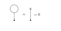
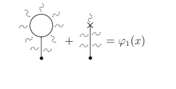
Figure 1: Renormalized tadpoles in the vacuum and in the kink background, respectively.

(ii) near the kink, the propagators of $\eta$ are deformed: they become (complicated) expressions for propagation in a kink background. Thus the cancellation of tadpoles which we imposed in flat space and which gave us the mass renormalization $\mu_{0}^{2}=\mu^{2}+\delta\mu^{2}$, no longer holds in the vicinity of the kink. Instead, one has in the kink sector

$$\varphi(x,t)=\varphi_{K}(x,t)+\varphi_{1}(x,t)+\eta(x,t),$$ (51)

where $\left<\eta(x,t)\right>=0$ by definition, and $\varphi_{1}(x)$ is a mean field induced by the kink [4]. This mean field gives another contribution to the energy density which we denote by $\Delta\epsilon_{(\varphi_{1})}(x)$ and which follows from expanding $\left<\mathcal{E}(x)\right>=\frac{1}{2}\left<\partial_{x}\varphi\partial_{x}\varphi\right>+\frac{1}{2}\left<U^{2}\right>$,

$$\Delta\epsilon_{(\varphi_{1})}(x)=\partial_{x}\varphi_{1}\partial_{x}\varphi_{K}+(\frac{1}{2}U^{2})^{\prime}\varphi_{1}=\partial_{x}(\varphi_{1}\partial_{x}\varphi_{K}).$$ (52)

The field $\varphi_{1}(x)$ follows from the vanishing of the expectation value of the field equation of the Heisenberg fields $\Phi$. Using $\left<\eta(x,t)\right>=0$ one easily obtains

$$\langle-\partial_{t}^{2}\Phi+\partial_{x}^{2}\Phi-(\frac{1}{2}U^{2})^{\prime}\rangle=0$$ (53)

$$=\partial_{x}^{2}\varphi_{1}-(\frac{1}{2}U^{2})^{\prime\prime}\varphi_{1}-\frac{1}{2!}(\frac{1}{2}U^{2})^{\prime\prime\prime}\langle\eta^{2}\rangle-\frac{1}{2}\delta m^{2}\varphi_{K}$$ (54)

The sum of the last two terms is again smooth and finite, and if we rewrite this equation as

$$\varphi_{1}(x)=\left[\partial_{x}^{2}-({\textstyle\frac{1}{2}}U^{2}){{}^{\prime\prime}}\right]^{-1}\langle\eta^{2}(x)-\eta^{2}(\infty)\rangle 3\lambda\varphi_{K}(x)$$ (55)

we recognise the Feynman graphs we depicted in Fig. 1.

The solution for $\varphi_{1}(x)$ is of the form $Ax\eta_{0}(x)+B\partial_{x}\eta_{0}(x)$ (note that $\left<\eta^{2}(x)\right>-\left<\eta^{2}(\infty)\right>$ contains terms with $\cosh^{-4}(mx/2)$ and $\eta_{0}\sim\cosh^{-2}(mx/2)$, and the fluctuation operator $\partial_{x}^{2}-({\textstyle\frac{1}{2}}U^{2}){{}^{\prime\prime}}$ vanishes on $\eta_{0}$). The term $Ax\eta_{0}(x)$ can also be written as proportional to $\varphi_{K}(x(1+A))$ because $\eta_{0}(x)\sim\partial_{x}\varphi_{K}$, and this rescaling of $x$ can also be written as a rescaling of $m$ (since $\varphi_{K}$ depends only on ${\textstyle\frac{1}{2}}mx$) and a counter rescaling of $\lambda$ to keep the prefactor $\mu/\sqrt{\lambda}$ invariant:

$$Ax\eta_{0}(x)\sim A(m\frac{\partial}{\partial m}+2\lambda\frac{\partial}{\partial\lambda})\varphi_{K}(x).$$ (56)

One can also write this as $\varphi_{K}(m,\lambda,x)+Ax\eta_{0}(x)=\varphi_{K}(\bar{m},\bar{\lambda},x)$ where we discover that this rescaling of the renormalized mass $m$ yields the pole mass $\bar{m}$ [4]! We have not been able to give a similarly simple physical explanation of the rescaled coupling $\bar{\lambda}=(\bar{m}/m)^{2}\lambda$.

One can now substitute all expressions to get explicit formulas for the complete energy density ${\mathcal{E}}(x)$ for the kink (or for any other 1+1 dimensional soliton). One can also repeat this exercise for the supersymmetric kink (in this case the only difference for $\varphi_{1}$ is a different result for $\bar{m}$ and $\bar{\lambda}$, but the term denoted by $B\partial_{x}\eta_{0}$ is the same). However, at this point we refer the reader to the original articles [4, 9].

The local central-charge density has been separately calculated for the susy case in [4] using higher derivative regularization, and also by using susy to transform the $\gamma\cdot j$ anomaly to the sector with the central charge. The explicit result for the local central-charge density of [4] agrees completely with the explicit result for the energy density of [9] (where also the explicit local energy density for the non-susy case is obtained). In [29] a calculation of the integrated central charge can be found in global mode regularization, with one cut-off for the Dirac delta function in the canonical equal-time (anti)commutation relations and another cut-off for the propagators; it is argued that these cutoffs should be the same and this indeed yields the correct result. In [9] the anomaly in the local central charge was obtained by starting from the definition

$$\zeta(y)=\int dx\,\delta(x-y)\{{\textstyle\frac{1}{2}}\varphi^{\prime}(x)U(y)+{\textstyle\frac{1}{2}}\varphi^{\prime}(y)U(x)\},$$ (57)

and not setting $x=y$ too soon. There is a $1/(x-y)$ singularity in the propagator $\langle\eta^{\prime}(x)\eta(y)\rangle$, and expanding $x$ around $y$ in the remaining terms, one finds a finite $(x-y)/(x-y)$ term which yields the anomaly.

So, in conclusion, the nonvanishing one-loop result for the energy density and total mass of the minimally susy kink as well as the associated nontrivial modification of the central charge (density) have been established in the various regularization methods. The specific subtleties of the different methods are now well understood, and the origin of the anomalous contribution to the central charge in each method clarified, which in particular in dimensional regularization and reduction shows most interesting facets.

Acknowledgments

It is a pleasure to thank the organizers for heroic achievements: a wonderful conference without glitches, an old-Russian-style banquet, and sleeping arrangements for all.

Appendix: The DHN program applied to fermions

The celebrated DHN calculation of the one loop corrections $M^{(1)}$ to the kink mass [1] due to bosonic fluctuations has been repeated in [15] for the fermionic case, using exactly the same steps as DHN did for bosons. We present this calculation here for two reasons: (i) to convince skeptics that there is indeed a problem with the fermions if one straightforwardly (or better: naively) repeats the same steps, and (ii) because there are subtleties with the zero modes which can be clearly illustrated by this concrete example. One might anticipate trouble by realizing that for supersymmetric boundary conditions (where all non-zero bosonic and fermionic modes cancel pairwise) the result for $\Delta M^{(1)}$ would be equal to only the counter term $\delta M$ which is divergent. Some physicists still feel uncomfortable with supersymmetry and prefer to stick to older “reliable” methods. The following explicit calculation should make it clear that these older methods need updating, for example along the lines suggested in the text.

The field equations for the fermions (= for the fermionic fluctuations) read$\not\!\!\partial\psi+U{{}^{\prime}}\psi=0$, where $U{{}^{\prime}}=\frac{\partial}{\partial\varphi}U(\varphi)$. In the representation $\gamma^{1}=\left({1\atop 0}{0\atop{-1}}\right)$ and $\gamma^{0}=\left({0\atop 1}{{-1}\atop 0}\right)$ the Dirac equation reads

$$(\partial_{x}+U{{}^{\prime}})\psi^{+}-\partial_{t}\psi^{-}=0\,,\ (-\partial_{x}+U{{}^{\prime}})\psi^{-}+\partial_{t}\psi^{+}=0\,,\ \psi=\left({\psi^{+}}\atop{\psi^{-}}\right).$$ (58)

Iterating and setting $\psi^{\pm}=u^{\pm}(x)e^{-i\omega t}$ yields

$$\left[\partial_{x}^{2}+\omega^{2}-m^{2}(\frac{3}{2}\tanh^{2}\frac{mx}{2}-\frac{1}{2})\right]u^{+}=0\,,$$ (59)

$$\left[\partial_{x}^{2}+\omega^{2}-m^{2}(\frac{1}{2}\tanh^{2}\frac{mx}{2}+\frac{1}{2})\right]u^{-}=0\,.$$ (60)

The equation for $u^{+}$ is the same as for the bosonic fluctuations $\eta$ ($\varphi=\varphi_{K}(x)+\eta(x,t)$), and hence before imposing boundary conditions, the solutions for $u^{+}$ are the same as for $\eta$. Given a solution for $u^{+}$ with $\omega\neq 0$, the Dirac equation gives the corresponding solution for $u^{-}$. From the shape of the potentials for the fluctuations (see Fig. 2), it is clear that $\eta$ and $\psi^{+}$ have a zero mode (a normalizable solution of the linearized equations for the fluctuations) but $u^{-}$ has no normalizable $\omega=0$ solution on $-\infty<x<\infty$. However, enclosing the system in a box $-L/2\leq x\leq L/2$, also $u^{-}$ has a zero mode.

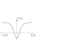
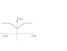
( $\eta$ )   ( $\psi^{+}$ )   ( $\psi^{-}$ )

Figure 2: Potentials for the one bosonic and the two fermionic fluctuation fields

For the bosonic fluctuations the zero mode $\eta_{0}\sim\cosh^{-2}(\frac{mx}{2})$ with strictly $\omega_{0}=0$ does not satisfy periodic boundary conditions because its derivative is odd in $x$, but by slightly increasing the energy $\omega$, we can achieve that its derivative vanishes at the boundaries. Hence, in the bosonic sector there is one almost-zero mode with $\omega_{0}^{2}\gtrapprox 0$. In the second-quantized expression for $\eta$ one finds then a term $(2\omega_{0})^{-1/2}(a_{0}\eta_{0}(x)e^{-i\omega_{0}t}+h.c.)$ which appears on a par with the genuine non-zero modes, and hence the almost-zero mode should correspond to one term in the sum over zero point energies, just as DHN assumed.

Imposing even boundary conditions on the fermions

$$\psi^{+}(-L/2)=\psi^{+}(L/2)\,,\quad\psi^{-}(-L/2)=\psi^{-}(L/2)\,,$$ (61)

we find the following mode solutions for $\omega\neq 0$:

$$\psi^{+}=\cos(kx\pm{\textstyle\frac{1}{2}}\delta^{+}(k))\cos\omega t \psi^{-}=-\sin(kx\pm{\textstyle\frac{1}{2}}\delta^{-}(k))\sin\omega t,\qquad$$ and (62)

$$\psi^{+}=-\sin(kx\pm{\textstyle\frac{1}{2}}\delta^{+}(k))\sin\omega t \psi^{-}=\cos(kx\pm{\textstyle\frac{1}{2}}\delta^{-}(k))\cos\omega t,$$ and (63)

with $\pm$ being a $+$ sign for large positive $x$ and a $-$ sign for large negative $x$. The Dirac equation is satisfied for $k\geq 0$ if

$$\textstyle\frac{k}{\omega}=\cos{\textstyle\frac{1}{2}}\theta(k)\,,\ \frac{m}{\omega}=-\sin{\textstyle\frac{1}{2}}\theta(k)\,,\ \delta^{-}(k)=\delta^{+}(k)+\theta(k),$$ (64)

where $\delta^{+}(k)=\delta_{K}(k)$ is the phase shift of the bosonic fluctuations. The solutions with $k<0$ are obtained from the solutions with $k>0$ by dropping the two minus signs in (62) and (63), but for $k<0$ (64) becomes $\delta^{-}(k)=\delta^{+}(k)+\theta(k)+\pi$ and thus the solutions with $k<0$ are the same as with $k>0$. The cosines satisfy the boundary conditions, but the sines must vanish at the boundaries. This yields two sets of quantization conditions on $k\geq 0$:

$$k_{n}^{+}L+\delta^{+}(k_{n}^{+})=2\pi n^{+},\ k_{n}^{-}L+\delta^{-}(k_{n}^{-})=2\pi n^{-}.$$ (65)

Given the shape of the phase shifts (see Fig. 3) it is clear that $n^{-}=1,2,3,\dots$, but $n^{+}=2,3,4,\dots$, because the solution with $n^{+}=1$ (yielding $k^{+}=0$) does not satisfy the boundary conditions.

    

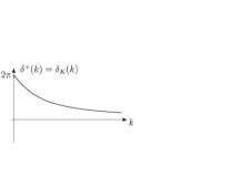
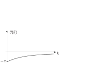
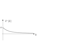
Figure 3: The phase shift functions $\delta^{+}\equiv\delta_{K}$, $\theta$, and $\delta^{-}=\delta^{+}+\theta$.

  

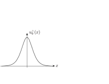
Figure 4: The fermionic zero modes $u^{+}_{0}(x)=1/\cosh^{2}(mx/2),u_{0}^{-}=0$ (concentrated at the kink) and $u_{0}^{+}=0,u_{0}^{-}=\cosh^{2}(mx/2)$ (concentrated at the boundary, if any).

We now turn to a closer study of the fermionic zero modes. They are both even, one concentrated near the kink and the other near the boundaries (see Fig. 4). Zero modes often correspond to symmetries of the classical action, but the fermionic zero mode which is concentrated on the boundary is an example of a zero mode which does not correspond to a symmetry, as one might expect since it ceases to be a normalizable zero mode on the infinite interval.

The mode expansions of the fermions read

$$\psi^{+} = \frac{1}{\sqrt{L}}{\sum_{n>0}}\left(c_{n}\frac{u_{n}^{+}(x)}{\sqrt{2}}e^{-i\omega_{n}t}+c_{n}^{\dagger}\frac{u_{n}^{+}(x)}{\sqrt{2}}e^{i\omega_{n}t}\right)+\frac{c_{0}u_{0}^{+}(x)}{\sqrt{L}}\,,$$ (66)

$$\psi^{-} = \frac{1}{\sqrt{L}}{\sum_{n>0}}\left(c_{n}\frac{u_{n}^{-}(x)}{\sqrt{2}}e^{-i\omega_{n}t}+c_{n}^{\dagger}\frac{u_{n}^{-}(x)}{\sqrt{2}}e^{i\omega_{n}t}\right)+\frac{d_{0}u_{0}^{-}(x)}{\sqrt{L}}\,,$$ (67)

where the sum over $n$ runs over both sets in (65), and where $u_{n}^{\pm}(x)$ are normalized to unit-strength plane waves $\exp i(k_{n}x\pm{\textstyle\frac{1}{2}}\delta^{\pm}(k_{n}))$ for large $\pm|x|$. Imposing the equal-time canonical anti-commutation relations $\{\psi^{\pm}(x,t),\psi^{\pm}(y,t)\}=\delta(x-y)$ one finds

$$\frac{1}{L}{\sum_{n>0}}\{c_{n},c_{n}^{\dagger}\}u_{n}^{+}(x)u_{n}^{+}(y)+\frac{1}{L}\{c_{0},c_{0}\}u_{0}^{+}(x)u_{0}^{+}(y)=\delta(x-y),$$ (68)

and a similar relation for $\psi^{-}$. To determine the value of the mode anti-commutators, we need a completeness relation for the mode functions $u_{n}^{+}(x)$, $u_{0}^{+}(x)$. We go back to the second-order differential equation for $\psi^{+}$, and imposing a second boundary condition which follows from the Dirac equation

$$\psi^{+}(-L/2)=\psi^{+}(L/2)\,,\ (\partial_{x}-m)\psi^{+}(-L/2)=(\partial_{x}+m)\psi^{+}(L/2)\,,$$ (69)

we obtain a bona-fide selfadjoint elliptic differential operator (with bosonic mode operators $a_{n}$ and $a_{n}^{\dagger}$), whose spectrum consists of $u_{n}^{+}(x)$, $u_{0}^{+}(x)$. This proves the completeness relation

$${\sum_{n>0}}\frac{1}{L}u_{n}^{+}(x)u_{n}^{+}(y)+\frac{1}{L}u_{0}^{+}(x)u_{0}^{+}(y)=\delta(x-y).$$ (70)

Comparing with (68) we deduce

$$\{c_{m},c_{n}^{\dagger}\}=\delta_{m,n}\,,\ \{c_{0},c_{0}\}=1.$$ (71)

The Hamiltonian density for fermions

$${\cal{H}}=\frac{i}{2}\psi^{T}\gamma^{0}(\gamma^{1}\partial_{x}+U^{\prime})\psi=\frac{i}{2}(\psi^{+}\partial_{t}\psi^{+}+\psi^{-}\partial_{t}\psi^{-})$$ (72)

yields the expected negative contribution to the zero-point energy, $\left<H\right>=\break-{\textstyle\frac{1}{2}}\hbar{\sum_{n>0}}\omega_{n}$, and in the density $\left<\psi^{+}(x)\psi^{+}(x)\right>$ the zero mode contributes a term ${\textstyle\frac{1}{2}}\frac{1}{L}u_{0}^{+}(x)u_{0}^{+}(x)$. Due to this factor ${\textstyle\frac{1}{2}}$, the two zero modes of the fermions in a box with even boundary conditions contribute one term to the sum over zero-point energies, just as for the bosonic case, and just as implicitly assumed by DHN.

We can now compute $\Delta M^{(1)}$. The fermionic modes cancel half of the bosonic modes for $n\geq 2$, but the bosonic $n=1$ mode is left. The bound states and the zero modes cancel between bosons and fermions. This yields

$$\Delta M^{(1)} = {\textstyle\frac{1}{2}}{\sum_{n\geq 1}}\omega(k_{n}^{+})-{\textstyle\frac{1}{2}}{\sum_{n\geq 2}}\omega(k_{n}^{-})+\delta M$$ (73)

$$= {\textstyle\frac{1}{2}}m+{\textstyle\frac{1}{2}}{\sum_{n\geq 2}}\frac{\partial\omega(k_{n}^{+})}{\partial k}\frac{\theta(k_{n})}{L}+\delta M$$

$$= {\textstyle\frac{1}{2}}m+{\textstyle\frac{1}{2}}\int_{0}^{\infty}\frac{dk}{2\pi}\frac{\partial\omega}{\partial k}\theta(k)+\delta M=\frac{\pi-2}{4\pi}m,$$

where we used that $k_{n}^{+}=k_{n}^{-}+\theta(k_{n}^{-})/L$. This is the correct answer to an incorrect question, because this value for $M^{(1)}$ contains spurious boundary energy. In the text it is discussed how to separate off the spurious boundary energy, and the correct result is

$$M^{(1)}=-\frac{m}{2\pi}\,.$$ (74)

If one repeats the same calculations for the sine-Gordon system, one can compare with the exact result obtained from the Yang-Baxter equation, and finds indeed that these two results agree after removing the boundary energy.

References

- [1] R. Dashen, B. Hasslacher, A. Neveu, Phys. Rev. D10 (1974) 4130.
- [2] J.-L. Gervais, A. Neveu (eds.), Phys. Rept. 23 (1976) 237.
- [3] L. D. Faddeev, V. E. Korepin, Phys. Rept. 42 (1978) 1.
- [4] M. A. Shifman, A. I. Vainshtein, M. B. Voloshin, Phys. Rev. D59 (1999) 045016.
- [5] A. S. Goldhaber, A. Litvintsev, P. van Nieuwenhuizen, Phys. Rev. D64 (2001) 045013.
- [6] H. Nastase, M. Stephanov, P. van Nieuwenhuizen, A. Rebhan, Nucl. Phys. B542 (1999) 471.
- [7] A. S. Goldhaber, A. Rebhan, P. van Nieuwenhuizen, R. Wimmer, Phys. Rev. D66 (2002) 085010.
- [8] J. F. Schonfeld, Nucl. Phys. B161 (1979) 125.
- [9] A. S. Goldhaber, A. Litvintsev, P. van Nieuwenhuizen, Local Casimir energy for solitons, hep-th/0109110 (2001).
- [10] R. Wimmer, Quantization of supersymmetric solitons, hep-th/0109119 (2001).
- [11] A. Rebhan, P. van Nieuwenhuizen, R. Wimmer, The anomaly in the central charge of the supersymmetric kink from dimensional regularization and reduction, hep-th/0207051, Nucl. Phys. B, in press (2002).
- [12] A. Parnachev, L. G. Yaffe, Phys. Rev. D62 (2000) 105034.
- [13] A. Rebhan, P. van Nieuwenhuizen, R. Wimmer, New J. Phys. 4 (2002) 31.
- [14] R. Rajaraman, Solitons and Instantons, North-Holland, Amsterdam, 1982.
- [15] A. Rebhan, P. van Nieuwenhuizen, Nucl. Phys. B508 (1997) 449.
- [16] W. Siegel, Phys. Lett. B84 (1979) 193.
- [17] D. M. Capper, D. R. T. Jones, P. van Nieuwenhuizen, Nucl. Phys. B167 (1980) 479.
- [18] C. G. Callan, J. A. Harvey, Nucl. Phys. B250 (1985) 427.
- [19] G. W. Gibbons, N. D. Lambert, Phys. Lett. B488 (2000) 90.
- [20] L. J. Boya, J. Casahorrán, Phys. Lett. B215 (1988) 753.
- [21] N. Graham, R. L. Jaffe, Nucl. Phys. B544 (1999) 432.
- [22] M. Bordag, A. S. Goldhaber, P. van Nieuwenhuizen, D. Vassilevich, Heat kernels and zeta-function regularization for the mass of the susy kink, hep-th/0203066, Phys. Rev. D, in press (2002).
- [23] R. K. Kaul, R. Rajaraman, Phys. Lett. B131 (1983) 357.
- [24] C. Imbimbo, S. Mukhi, Nucl. Phys. B247 (1984) 471.
- [25] A. Chatterjee, P. Majumdar, Phys. Rev. D30 (1984) 844; Phys. Lett. B159 (1985) 37.
- [26] H. Yamagishi, Phys. Lett. B147 (1984) 425.
- [27] A. Uchiyama, Prog. Theor. Phys. 75 (1986) 1214.
- [28] C. Ahn, Nucl. Phys. B354 (1991) 57.
- [29] A. Litvintsev, P. van Nieuwenhuizen, Once more on the BPS bound for the susy kink, hep-th/0010051 (2000).
- [30] G. W. Gibbons, P. K. Townsend, Phys. Rev. Lett. 83 (1999) 1727.
- [31] A. Losev, M. A. Shifman, A. I. Vainshtein, New J. Phys. 4 (2002) 21.
- [32] G. Bonneau, Nucl. Phys. B167 (1980) 261; Nucl. Phys. B171 (1980) 477.