On the Moduli Space of SU(3) Seiberg-Witten Theory with Matter

Abstract:

We present a qualitative model of the Coulomb branch of the moduli space of low-energy effective ${\cal N}=2$ SQCD with gauge group SU$(3)$ and up to five flavours of massive matter. Overall, away from double cores, we find a situation broadly similar to the case with no matter, but with additional complexity due to the proliferation of extra BPS states. We also include a revised version of the pure SU$(3)$ model which can accommodate just the orthodox weak coupling spectrum.

1 Introduction

There was much excitement caused by the seminal papers of Seiberg and Witten [1, 2] in which they found exact non-perturbative results for low-energy effective ${\cal N}=2$ supersymmetric gauge theories. A wide array of authors have expanded upon the initial work [4, 5, 6, 10, 11, 20, 21, 23, 24], both in fleshing out further detail within the SU$(2)$ case, and also boldly entering into the domain of the higher gauge groups. It is no less apparent now than originally that these results are more than those of a toy model, but rather present an iconic paradigm, a nugget of solidity up against which most new abstract theories must be measured. It has already been generalised and deformed in a myriad of ways, and we expect this to continue in the years to come. We consider it important, therefore, to work through some of the remaining details in the more complex, but still amenable cases. In particular, the example of SU$(3)$ is one which merits attention, being both the simplest case where the two Higgs scalars of the theory generically misalign in group space; and, of course, due to the links with the usual conundrum that is QCD.

In [3] we presented a plausible, consistent qualitative model of the curves of marginal stability that exist in the moduli space of pure SU$(3)$ Seiberg-Witten Theory. In addition to modifying this slightly, we shall now show how this generalises to the cases with up to five matter multiplets in the fundamental representation of the gauge group.

In each case we have a four real-dimensional space which we choose, following [21], to write as a fibration of concentric three-spheres. There exists a surface of points on which this abelian theory breaks down due to extra fields becoming massless. The intersection of this with a three-sphere with radius larger than a critical value comes in the shape of a knot called a trefoil. In the pure case there is an instanton effect which exacts a bifurcation of the classical trefoil. For $N_{f}$ flavours, this local bifurcation patches together non-trivially - there are $N_{f}$ half-twists as we traverse the classical knot (so for odd $N_{f}$ we retain one, more complicated, knot). In addition there are in general $N_{f}$ singular curves corresponding to where the quarks (with non-degenerate bare masses) become massless. These are generally planes, which therefore intersect our three-sphere as circles, until we increase the bare masses sufficiently whereupon they shrink to point before giving a null intersection.

At a point of weak coupling, we have the BPS spectrum first given in [8]. This consists of massless gauge bosons plus the same towers of dyon hypermultiplets as in the pure case; the quark hypermultiplets, often with bare mass; and massive gauge bosons which can be thought of as bound states of two of these. Finally, the largest set of states are bound states of dyons and quarks. Each dyon can bind in up to $2^{N_{f}}$ combinations.

As we increase the coupling, there exist hypersurfaces past which some BPS bound states are no longer stable. In a region of moderate to strong coupling, we see most of the dyon-quark states lose stability. Curiously, the flavour singlet states consisting of a dyon together with one of each flavour quark remain stable into the regions of strong coupling in root directions not equal to the magnetic charge of that dyon. This is true subject to the proviso that the dyon is stable in that region. In analogy with the pure SU$(3)$ example, there are single cores, where one abelian gauge symmetry is strongly coupled; and double cores where both are. In the single core, one of the towers of dyons, except for two of its elements, loses stability; and the other two towers are transformed. In the double core, most of these others become unstable too, and we are left with a finite spectrum. We have such cores in all the examples. The only addition to the spectrum now is that of all the quarks (and some states into which they can transform when passing through a branch cut), plus the flavour singlet bound states with dyons of the reduced spectrum.

We have produced this somewhat sketchy atlas as a first attempt to gain a concrete understanding of these moduli spaces. Hopefully this will inspire a more rigorous study by the more determined or enlightened. Our findings contain nothing startlingly contentious and are self-consistent. Our weak coupling spectrum is orthodox, following [26]. Our strong-coupling spectrum agrees with that of [8] at the point where they show it must be dual to that of the $\mathbb{CP}^{5-N_{f}}$ sigma model, for $6>N_{f}\geq 3$. We present what we believe lies in between. However, we feel we should point out before proceeding that this study is but a tower of logic crying out for the firm basis a plot of these curves would provide.

Thus we begin in Chapter two with a review of the pure case, in which we include the slight modifications to SU$(3)$ SYM. In Chapter three we sketch the SU$(2)$ picture in the same manner as for SU$(3)$ in order to allow for comparison, then we consider in detail the case with one flavour. In Chapter four we deal mainly with the example of three flavours to show the pattern followed by all the rest. Chapter five looks at what must happen as we flow between the various examples. We conclude with a brief discussion of how we agree with other work.

2 The pure case revisited

2.1 Classical Model

Let us begin with a review of the pure SU$(3)$ model, further details can be found in [3]. SU$(3)$ is a group based on an eight-dimensional Lie algebra, within which we find embedded in the standard way three copies of SU$(2)$. We think of these as lying along the root directions of the Cartan subalgebra (CSA), which are harmoniously arranged within a plane to give hexagonal symmetry. An SU$(N)$, ${\cal N}=2$ gauge theory has two adjoint Higgs fields in its gauge multiplet. We consider only the Coulomb branch, at a generic point of which these spontaneously break the gauge symmetry to its maximal torus. The vacuum expectation values of these determine the parameters of each theory. We range over them as we seek to determine the moduli space of supersymmetric vacua, and at each point also we require the spectrum of excited states that are BPS and so amenable to us of the second superstring revolution. Gauge-fixing transformations allow us the freedom to conjugate these vevs into the maximal torus, so we can restrict ourselves to the (complexified) CSA (then exponentiate). Even so, generically the two Higgs fields do not align. If either lies perpendicular to a root direction we have trouble. Dark (non-abelian) clouds loom if our adjoint Higgs do not induce spontaneous symmetry breaking of SU$(3)$ down to U$(1)\times$ U$(1)$. Seiberg and Witten [1] showed that this manifests itself at the boundary of the closure of the moduli space where a field that we have considered massive in the effective theory becomes massless, conveying the effect of the symmetry restoration. We call this set the singularity curve (though our sections of it may make it seem disconnected into many curves). It can be determined as the zero set of a high-order polynomial in the coordinates we choose for the moduli space. As a surface it has singularities in the mathematical sense. Thankfully, for SU$(3)$ these are only points. Particularly interesting conformal field theories often lie here, however [21], and the areas of the moduli space with a finite stable BPS spectrum, nearby.

The complexified CSA of SU$(3)$ has four real dimensions, which we parameterise by two complex variables, $u$ and $v$, the quadratic and cubic Casimirs of the algebra, natural as these are Weyl group invariant, a symmetry left over after gauge fixing to the CSA. They have mass dimensions of two and three respectively. All the classes of theories have a dynamically generated scale $\Lambda$ (although it depends on $N_{f}$ and their masses). Setting this to zero eliminates the non-perturbative effects and is what we mean by the ‘classical case’ (1-loop perturbative would be more accurate). Here the singularity curve is given by $4u^{3}=27v^{2}$. Following [21] we find the intersection with the (topological) 3-sphere defined as $4|u|^{3}+27|v|^{2}=R^{6}$. This means that $u$ and $v$ are of constant length and cycle (on a torus) in the ratio $3:2$.

Figure 1: The classical trefoil ${\cal T}_{cl}$ wrapping three times around one cycle as it wraps twice around the other.

Physical quantities are obtained not from $u$ and $v$, but from appropriate linear combinations of the complex 2-vectors $a$ and $a_{D}$, where $a$ is the vev of the Higgs. These are more accurately sections of an Sp$(4,\mathbb{Z})$ bundle over the moduli space, and they show up in the central charge of the algebra, which relates to the energy of BPS states. The rest mass of a BPS state $(g,q)$ with magnetic charge $g$ and electric charge $q$ is given by

$$m[(g,q)]=|g.a_{D}+q.a|.$$ (1)

Upon circling any hole in the moduli space, $(a,a_{D})$ is acted upon by an element of Sp$(4,\mathbb{Z})$. Obviously $(g,q)$ must be acted upon by the inverse element of Sp$(4,\mathbb{Z})$ to maintain the mass. Pick a basis $\{(g_{1},q_{1}),\dots,(g_{n},q_{n})\}$ of states that become massless at the singularity we are circling, then the transformation matrix is singled out as a product of ones of the canonical form for each element

$$M_{(g,q)}=\left(\begin{array}[]{c|c}1+q\otimes g&q\otimes q\\ \hline\cr-g\otimes g&\mbox{\hskip 5.0pt}1-g\otimes q\end{array}\right).$$

We are free to choose where to enact this transformation on the charges (and $a$ and $a_{D}$), but somewhere we must decide to put a branch cut (which is one real-codimensional) emanating from the (one complex-codimensional) singular curve. We must also decide where we would like it to go. For simplicity we shall make most of our cuts meet at the origin.

As well as gauge bosons, we learn from [17, 18, 9, 26] among others that the weak-coupling spectrum includes dyons in massive ${\cal N}=2$ hypermultiplets. The magnetic charge of each dyon must be root-valued, i.e. has charge $\alpha_{1},\alpha_{2}$ or $\alpha_{3}$ (if it is negative, its CP conjugate, which will also be present will be positive, so we take this). These occur in towers, with one of each root coexisting at each point. The tower of the non-simple root out of these (defined as the sum of the two obtuse roots having positive scalar product with the dominant principal direction of the Higgs fields) is comprised of stable bound states of the other two and is slightly different. The other, more basic two, are simply embeddings of the SU$(2)$ dyons in the simple root directions and as such have electric charge in integer multiples of their magnetic charge. The electric charge of the third tower is ‘offset’. Each state is a bound state of $n$ units of one root with either $n+1$ or $n-1$ of the other. These two bound states do not co-exist and hence form two distinct weak-coupling limits (in our picture, these correspond to the origin and infinity). For definiteness, we shall concentrate on the third of the moduli space for which $\alpha_{3}$ is non-simple. This has regions, among others, extending from the two limits containing the states

$$Q_{1}^{n}=(\alpha_{1},(n-1)\alpha_{1})\hskip 5.0pt,\hskip 5.0ptQ_{2}^{n}=(\alpha_{2},n\alpha_{2})\hskip 50.0ptQ_{1}^{n}=(\alpha_{1},(n-1)\alpha_{1})\hskip 5.0pt,\hskip 5.0ptQ_{2}^{n}=(\alpha_{2},n\alpha_{2})$$

$$Q_{3-}^{n}=(\alpha_{3},-\alpha_{1}+n\alpha_{3})\hskip 50.0pt\mbox{\raisebox{5.0pt}{ or }}\hskip 55.0ptQ_{3+}^{n}=(\alpha_{3},+\alpha_{1}+n\alpha_{3}).$$

More recent work [12, 13, 14] has shown that BPS states in higher spin multiplets can also exist here. Towers of these have the non-simple root as magnetic charge, and can be thought of as bound states of a dyon of each simple root with $n$ units of one root and $n+m$ or $n-m$ $(m>0)$ units of the other, depending in which weak coupling-limit we are located. Thus for the highest root the electric charge can range over the whole root lattice, although only half at any particular point.

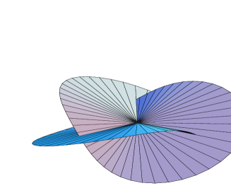
Figure 2: The classical branch cuts form a self-intersecting surface.

Returning now to the branch cuts, these can be placed between the trefoil and the origin to form a self-intersecting surface as in fig. (2). The transformations, called monodromies, are labelled $N_{i}$. If we denote by $[(g,q)]$ the canonical monodromy associated to $(g,q)$, then

$$N_{i}=[Q_{i}^{n}][Q_{i}^{n-1}].$$

Where we use $Q_{3-}$ for $i=3$ (though, in fact we add should include additional branch cuts as detailed in [3], such that we only ever need use simple root monodromies, but we shall ignore these as we are concentrating solely on when $\alpha_{3}$ is non-simple).

It is obvious from the diagram that we need a mechanism whereby $Q_{3+}$’s which are present at the origin, and $Q_{3-}$’s which are present at infinity, cease to exist in the other region (as stable BPS bound states). This must happen on the border of when it is energetically favourable for the bound state to exist, which in this case is simply when the mass of the bound state is equal to the sum of the masses of its constituents. This occurs in this case when our two Higgs fields align. Topologically this real-codimension one surface, called a curve of marginal stability (CMS), is a twisted ribbon as in fig. (3).

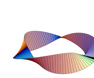
Figure 3: The classical CMS.

Let us take radial sections of this picture in order to help visualise things, whilst bearing in mind that we may often need to rotate this section through $2\pi$ to check consistency (see fig. (4)).

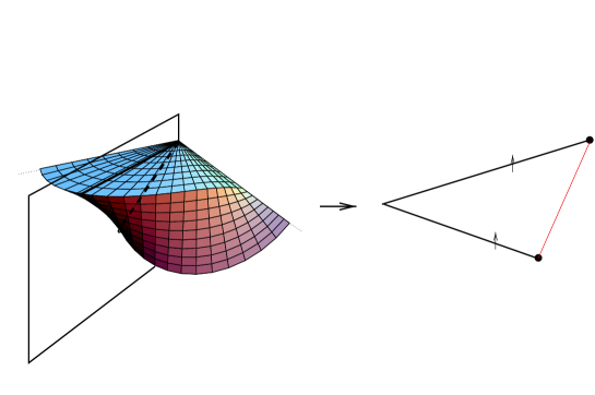
Figure 4: We take radial sections.

We now modify the model of [3] with the addition of other such CMS’s. Upon these, the states in higher spin multiplets with electric charge $(n+m)$ or $(n-m)$ units of one simple root decay to $(n+1)$ or $(n-1)$ together with $(m-1)$ copies of the appropriate massive gauge boson. These take the shape of just a small and a large sphere in our model. See fig. (5) for the details of how the remaining dyons are partitioned by these cuts and CMS’s into two regions $3+$ and $3-$.

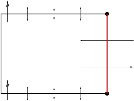
Figure 5: The classical BPS spectra in the $3+$ and $3-$ domains.

2.2 Instanton Corrections

In ${\cal N}=2$ gauge theories non-perturbative corrections are due to instantons, and are proportional to positive integer powers of the dynamically generated scale $\Lambda$. At strong coupling these effects dominate and the model is best expressed in terms of a dual abelian gauge theory with weak coupling. In the original theory we are considering 3-spheres of radius $R$. Large $R/\Lambda$ corresponds to weak coupling. Decreasing from infinite $R/\Lambda$, the trefoil splits in two, and a new quantum monodromy is formed between them. This is analogous to the case for SU$(2)$ where classically one singularity splits into two with a cut formed between them. Also like in this case, a new, closed CMS is formed, signalling the loss of stability inside the curve for a BPS state with a particular charge, in fact for an infinite number of cases of charge. We call the structure from which the monodromy $N_{i}$ extends to the origin the $\alpha_{i}$ arm. From the point of view of the states charged only with $\alpha_{i}$ this is a carbon copy of the situation for SU$(2)$, which is only to be expected as the dyons are nothing more than SU$(2)$ embeddings along the sub-SU$(2)$ corresponding to this root. This is illustrated in fig. (6).

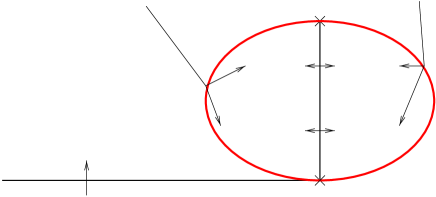
Figure 6: The region where the $\alpha_{i}$ direction is strongly coupled.

As we rotate our radial section, the two arms rotate around each other, and the region inside the new curve remains bounded from the outside. The CMS, which we shall call $L$ for local (and $L_{i}$ the subset on the $\alpha_{i}$ arm) forms a tube in the shape of the classical trefoil as in fig. (7). Inside the tube is the core, a region of moduli space with a much reduced BPS spectrum. As illustrated in fig. (6), on each arm, from a given direction a single state becomes massless on each trefoil. We have chosen the branch where $Q_{i}^{1}$ does so at the top. The spectrum of states with magnetic charge $\alpha_{i}$ in the hemi-tube along the $\alpha_{i}$ arm will consist only of the two states which become massless in that section, this is reasonable as they are light. In [3] we suggested a mechanism whereby the states in the other two towers are transformed or split into three (two co-existing at any point) differently charged towers of states which are relatively light at this arm. This duty is discharged by the remnant of the ribbon-like CMS. Adding quantum corrections it splits into an infinite number of curves, which we call the $G$’s (for global), each delineating the boundary of stability of one of the $Q_{3\pm}$’s.

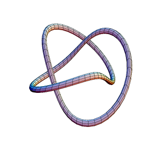
Figure 7: The CMS $L$ which bounds the core.

We define

$$S_{m,i}^{\mbox{-}1} = Q_{i-1}^{2n+1}N_{i}^{m}$$

$$S_{m,i}^{0} = Q_{i-1}^{2n+2}N_{i}^{m}$$

$$S_{m,i}^{1} = Q_{i-1}^{2n+3}N_{i}^{m}.$$ (2)

Within the core on the $\alpha_{i}$ arm we have the states as in the left hand of fig. (8). In order to generalize simply, we would like to change where we put the cuts $N_{i}$. Instead of always linking to the bottom trefoil, we shall link to the centre. This now gives us three regions of core with indices in the new region just one higher than those on the right, and two greater than those on the left, as depicted in the right-hand diagram. We could have done this for SU$(2)$ also, and indeed sometimes it is more natural so to do this, such as when mapping from the fundamental domain of $\Gamma(2)$.

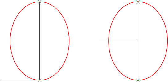
Figure 8: States in the single core with old and new cuts

If we continue to decrease the radius of our three-sphere, eventually the trefoils will be so far apart that it will become impossible for them (and $L$) not to self-intersect. Note that it is always different arms which intersect, and hence we interpret this as where both gauge U(1)’s are strongly coupled. We maintain that the cores cannot just pass through one another with their intersection supporting the intersection of the two cores for each arm. Rather, they amalgamate, like a crossroads junction in a sewer, and concentric spheres of entirely new curves block the contents of each tube from the other. In the centre of the junction, inside these new curves, lies a smaller, finite spectrum of BPS states common to both of the intersecting cores. We call these spaces the double cores. They exist in the vicinity of both the $A_{1}$ and $A_{2}$ singularities of the singularity surface.

Although the curves and states listed in [3] are consistent, we have little way at present of knowing what precisely is happening at such strong coupling. We now believe that a more simple scenario is more likely to occur. It involves allowing a further branch cut $V$ to open up and straddle the intersection of the tubes. $V$ consists of just the $\alpha_{3}$ Weyl reflection in both electric and magnetic sectors. We sketch how this may occur (ignoring the $S$’s) in fig. (9). Note that the curves around the double core now work for an infinite number of $m$ at the same time, similarly to the $L_{i}$ for the $n$. One might expect a decay into the $S$ of lowest possible $m$, i.e., $S_{2m,i}\rightarrow mS_{0,i}-(m-1)S_{\mbox{-}2,i},\,\,S_{2m+1,i}\rightarrow mS_{1,i}-(m-1)S_{\mbox{-}1,i}$. This would leave ten states at each point of the double core. We believe there should be six. As odd and even $m$ behave separately, each would still differ in electric charge by twice $P_{i}=\alpha_{i+1}-\alpha_{i-1}$ (e.g.  around the $\alpha_{1}$ core we have $P_{1}=\alpha_{1}+2\alpha_{2}$). In fact they can, and do decay to states only one $P_{1}$ apart. Four of these are new to us, in the $\alpha_{1}$ part: $(Q_{2}^{0}+P_{1}),(Q_{2}^{1}+P_{1}),(\alpha_{3},0)$ and $(\alpha_{3},\alpha_{3})$. The other four in this area are $S_{\mbox{-}1,1}^{0},S_{\mbox{-}1,1}^{1},S_{0,1}^{0}$ and $S_{0,1}^{1}$. The extra four states exist only inside a spherical ‘bubble’ and lose stability on one curve each. These mark the boundary of the double core, passing through both accumulation points, but also extend to touch one of the singularities of the $\alpha_{i}$ core. In fig. (10) we show a double core at one particular phase of the intersection.

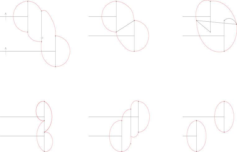
Figure 9: How $V$ moves as cores intersect, including the effect on some states

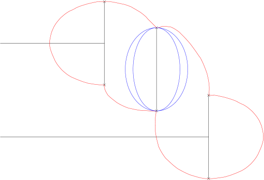
Figure 10: States in the double core (centre) with monodromy $V$

As we continue to shrink our three-sphere smaller than the radius where the singular points of the singularity curve occur, we find that the knot has become disentangled into three circles, each with a core relating to a single arm and all the other accoutrements of that arm, including the $N_{i}$ monodromy running in to the centre of this circle. Eventually these circles shrink to a point then disappear.

3 One flavour and preliminaries

3.1 Matter matters

The addition of fundamental matter in the SU$(2)$ case is rather less illustrative of the general scenario than that for pure vector-multiplets. Seiberg and Witten [2] make sure to include a factor of two in a change of conventions when hypermultiplets in the fundamental are included. This is actually the action of the Cartan matrix of SU$(2)$ on the electric sector of the theory, required because now the electric charges of dyons and quarks take values in the weight lattice of the group, as opposed to just the root lattice before. This linear map also transforms the weights back into a multiple of the roots (as they are dual) and corresponds to the isogeny of the jacobian of the auxiliary elliptic curve. It is not necessary for us to change conventions at all unless we want explicit representations of the monodromy matrices, and even then not needed if, as we have previously, used the far-sighted conventions of [10, 11, 20].

In SU$(2)$, the weight and root lattice are necessarily collinear, making it difficult to discern whether a state is a bound state of a dyon with two quarks with equal and opposite bare mass, or just the dyon with the next highest charge. Here, SU$(3)$ is more transparent. SU$(2)$ also has non-standard flavour symmetry. For $N_{f}$ massless hypermultiplets this symmetry expands from the usual U$(N_{f})$ to O$(2N_{f})$. Again, SU$(3)$ is free from this complication.

Following the impressive progress one can make in the pure case of looking for SU$(2)$ embeddings, charting where they must lead and the implications, one might be hoping for similar inspiration here. Sadly, of course, prospective SU$(2)$ weights, lying along root directions with half-integer spacing, are not SU$(3)$ weights, which lie at the vertices and centroids of the equilateral triangles formed by the root lattice. Thus we can infer that searching for embeddings of the states, multiplicities, monodromies and superconformal points as detailed in [4, 5, 6] is folly. Rather, the extra singularities which become those where very bare-massive quarks become massless stay well out of the way, for the most part, of the pure SU$(2)$ embeddings and the core.

The new feature of these extra singularities is that upon traversing a path around them $a$ and $a_{D}$ pick up an integer multiple of the bare mass of the state which becomes massless at the singularity. The flavour symmetry in the generic case is a global U$(1)^{N_{f}}$, and all of the BPS states can be thought of as carrying additional quantum numbers, having an integer charge under each of these U$(1)$’s. We can think of these as ‘merging’ when two bare masses become degenerate, summing the old charges. We can then extend the canonical labelling of monodromies. A state with charges $(g,q)_{s}$, with $s=(s_{1},\dots,s_{N_{f}})$ which becomes massless has the associated monodromy

$$M_{(g,\,q)_{s}}=\left(\begin{array}[]{c|c|c}1+q\otimes g\mbox{\hskip 5.0pt}&\mbox{\hskip 3.0pt}q\otimes q\mbox{\hskip 2.0pt}&\mbox{\hskip 8.0pt}s\otimes q\\[3.0pt] \hline\cr\raisebox{13.0pt}{}\mbox{}-g\otimes g&\mbox{\hskip 5.0pt}1-g\otimes q\mbox{\hskip 2.0pt}&\mbox{\hskip 2.0pt}-s\otimes g\\[3.0pt] \hline\cr\raisebox{12.0pt}{}0&0&\mbox{\hskip 2.0pt}1\end{array}\right).$$

Quarks necessarily have one unit of s-charge, but are varied in their choice of which of the $s_{i}$ to have. Generically, for each weight of the fundamental representation of the gauge group, we will find $N_{f}$ hypermultiplets with that electric charge, each with a different $s_{i}$ being non-zero. One sensible computational basis of weights is that dual to the simple roots, which has $(N-1)=2$ elements. It can be more instructive for SU$(N)$ to use the fact that each of the $N(N-1)$ roots can be expressed as a different difference of two of the $N$ weights of the fundamental representation. Physically, this means here that each gauge boson can be considered a bound state of a quark and antiquark (of the same flavour).

Each matter hypermultiplet contains a colour triplet of quarks. We label our three quarks by their electric charge: $\lambda_{1}$, $\lambda_{2}$ and $\lambda_{3}=-(\lambda_{1}+\lambda_{2})$, where the lambdas are the three weights of the fundamental, $\alpha_{1}=\lambda_{2}-\lambda_{3}$ and cyclic permutations. If flavours have different masses, then we need a further label to distinguish each set of different mass. We give each an s-charge, of one, under the U$(1)$ part of the flavour symmetry this subset possesses. This quantity shows up in the central charge, with $a$ and $a_{D}$, multiplied by the corresponding bare mass (with a factor of $(1/\sqrt{2})$ which we can safely ignore in this qualitative approach). This, of course, just has the effect of adding the bare mass to the central charge, the modulus of the total now being the mass of a state at a particular point of the moduli space. Following the example of [5] we could label the s-charges of a state as an $N_{f}$-tuple of subscripts following the other charges, e.g., $(g,q)_{s_{1},\,s_{2},\,\dots,\,s_{N_{f}}}$, but as the charge is always $+1$ for quarks (and of obvious sign for other states), we prefer to write, for example, $(g,q)^{ac}$ for $(g,q)_{10100\dots}$.

We will later require notation to enumerate the quark-dyon bound states. We will find dyons with magnetic root $\alpha_{1}$ bind to the weight orthogonal to this, which in our notation is labelled $\lambda_{2}$. As $\lambda_{2}-\alpha_{1}=\lambda_{3}$, any such state could also be thought of as a bound state with $\lambda_{3}$. We shall always label it relating to the first possibility. We draw a bar over the name of the dyon for each such quark bound with it, and add the s-charge labels appropriately. Antiquarks are also apt to form bound states, we then add lower bars. In a similar way, we add an upper bar for each $\lambda_{1}$ bound with $\alpha_{2}$ dyons, and for each $\lambda_{1}$ with all $\alpha_{3}$ dyons.

$N_{f}$	rotation fraction
$0$	$1/3,\,1/2$
$1$	$2/5,\,3/5$
$2$	$1/2,\,3/4$
$3$	$2/3,\,1$
$4$	$1,\,1/2$
$5$	$1,\,1$

Table 1: duality symmetries

The pure SU$(2)$ moduli space described by quadratic Casimir $u$ has a discrete $\mathbb{Z}_{2}$ duality symmetry, and with $N_{f}$ masses $\mathbb{Z}_{4-N_{f}}$. By this we mean the theories at $u$ and $ue^{2\pi i/(4-N_{f})}$ will be dual descriptions of the same physical theory. The order of the group is related to the anomaly-free subgroup of the classical U$(1)_{R}$ symmetry (and also parity), which is $\mathbb{Z}_{4(4-N_{f})}$ except for zero flavours where it is $\mathbb{Z}_{2(4-N_{f})}$. Note $u$ has charge $4$ under this symmetry, thus we have the stated invariance. For SU$(3)$ we also get such dualities - just replace $4(4-N_{f})$ with $2(6-N_{f})$, and include $v$ with charge $6$. Therefore the symmetries occur for simultaneous rotation of $u$ and $v$ by the amounts listed in Table 1. In particular, singularities of the singular curve, and also the existence of cores and double cores will respect this symmetry.

3.2 SU$(2)$ with Generic Masses

In [6], Bilal and Ferrari describe in much detail and list a compendium of relevant CMS’s for the case of two flavours with equal real positive bare masses, and a choice of branch cuts partly decided by the constraints of computational practicality. They show the consistency of their description and are solidly backed by the results of their methodical numerical study of exactly where these CMS’s lie. We free ourselves of these restrictions such that we may present as simple as possible a picture as we can muster. The case with four flavours is special and is dealt with in [7].

The moduli space is always a punctured complex plane. We begin without matter. There exists a core region about the origin. On the boundary of this are two singularities in which states of charge $(1,0)$ and $(1,2)$ respectively become massless. Inside the core, only two states exist at any point, outside, $(1,2n)$ for all $n$, and the vector-multiplet $(0,2)$. From the core to infinity there exists a branch cut with monodromy

$$M_{\infty}^{4}=\left(\begin{array}[]{cr}-1&1\\ 0&-1\end{array}\right)^{4}=\left(\begin{array}[]{cr}-1&4\\ 0&-1\end{array}\right).$$

We can add up to four hypermultiplets in the fundamental representation of the gauge group without destroying the asymptotic freedom of the theory. If we give them bare masses $m_{i}$, as we take these masses to infinity, the multiplets decouple and we return to the pure case. Moreover, we expect to see this changeover to the pure structure occurring first at a scale small compared to the bare mass, and then increasing to infinity as the mass does. Thus, for $N_{1}$ masses varying, after a brief period of bare mass of order $\Lambda$ where the extra singularity is in the strong coupling region, increasing $|m_{i}|$ it disentangles itself from the $N_{f}$ core structure to leave behind the $N_{f}-N_{1}$ core structure, and, if we look at the generic case when all the multiplets have sizeable bare mass, the pure core structure. We encumber this concept with the pious tag ‘purity comes from within’.

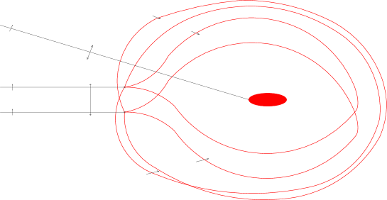
Figure 11: Generalised sketch of SU$(2)$ with matter

If we accept the argument that the set of stable states for $N_{f}$ flavours is a subset of that for $N_{f}+1$, then necessarily we find that closed curves of marginal stability must emanate from each extra singularity, encircling the core, forming the boundary of the existence domain of states unwanted within. The monodromies across the branch cuts of each of the $N_{f}$ extra singularities are of the form $[(0,1)_{0,\dots,1,\dots,0}]$ with the non-trivial s-charge lying in each position once and only once. These act on a dyon of unit magnetic charge by adding exactly this charge to the charges of the dyon. In this way we see the existence of quark-dyon bound states which carry s-charge. Note that there will exist one of the closed CMS’s upon which this bound state is no longer stable (so one cannot repeatedly encircle one of these singularities and get a bound state of arbitrarily high s-charge). Quarks are not affected by these monodromies, so they commute with each other. Combined with $M_{\infty}^{4}$ we get a total monodromy that would be $M_{\infty}^{4-N_{f}}$, but it includes one each of the s-charges. Notice that $M_{\infty}^{4}$ includes the transformation that Seiberg and Witten [2] call $P$ which negates $a$ and $a_{D}$, and hence in our notation negates all the s-charges. Rotating a dyon about infinity, we would first pick up one each of positive s-charges, then cross $M_{\infty}^{4}$ to see them become all $-1$’s. Recrossing the quark monodromies we would gain charge again to get back to zero. Thus we do not get arbitrarily high s-charge from this rotation either. From a glance at fig. (11) we see that at any point only $2^{N_{f}}$ different s-charge combinations are allowed. In one of the two largest spaces it is the case that every s-charge can (independently) be $0$ or $+1$; in the other, that it can be $0$ or $-1$. Between the quark monodromies we get mixtures.

3.3 SU$(3)$ with one flavour

We know that for higher gauge groups the negation property of $M_{\infty}^{4}$ generalises as a Weyl reflection. In SU$(3)$ each of the $N_{i}$ makes such a transformation, effectively negating $a$ and $a_{D}$ in the $\alpha_{i}$ direction, and swapping without negation, the other two root directions. We need the extra monodromy we get when we add one flavour to interact with these, as we saw for SU$(2)$, to restrict the s-charges to $\{0,\pm 1\}$. The position of the extra singularity for zero bare mass is easily calculated and is found to be a circle inside the torus on which the classical trefoil lies. We take the branch cut from this circle to extend to its centre at the origin. We should then take the monodromy to be $[(0,\lambda_{3})_{1}]$ as this is weight of the fundamental representation which is orthogonal to $\alpha_{3}$, (the 3’s only coincidentally corresponding — they are the only things that are not $1$ or $2$) the only root in the fundamental Weyl chamber, to which the dominant principal direction of the Higgs fields is restricted for this discussion. As can be seen from fig. (12), we now have three regions and an expanded BPS spectrum within each. $Q_{3}$’s exist only barless or with upper bars. The $\bar{Q}_{2}$’s exist in the $3-$ and the upper of the two $3+$ regions, and may move freely between them. Instead, however, $\underline{Q}_{2}$’s exist in the lower $3+$, and the both of them are marginally stable to $Q_{2}$’s and $\pm(0,\lambda_{1})_{1}$ (this couldn’t happen simultaneously in the quantum case, but we have extreme degeneracy in this limit). Similarly $\underline{Q}_{1}$’s exist only in the upper $3+$.

Figure 12: The picture for one flavour at $\Lambda/R=0$

3.4 Non-perturbative Effects: Small $\Lambda$

We now add in non-perturbative effects, staying in the regime $R\gg\Lambda$ where these are small. The extra monodromy changes many things. The global curves which in the pure case partitioned the space into two now pass through this extra branch cut and are altered accordingly. They cannot now partition all the varied states we have, and one further set of curves is necessary to complete the picture, but we shall see that they do so for all the $Q_{3}$’s. Without the matter, in [3] we showed that in our usual radial section just two small segments were needed to generate all the curves. Now we need several more. The picture which works is illustrated in fig. (13), where both left acting and right acting curves that we had included before are present, bending to the outside of the singularity. A global clockwise rotation of the arms by three half twists, also including the local half-twist in one core, returns our radial section to the same place but leaves the former curves in a different position, now passing to the inside of the singularity, through the monodromy. Repeating, they return outside, but with different index $n\rightarrow n-5$. Thus five copies of the two original curves are needed to generate all $n$. This is all that is necessary to partition all the $Q_{3}$ and $\bar{Q}_{3}$’s. At the cores we now have a whole set of $G$ as in the pure case, and also a whole set of $\bar{G}$’s which act on the $\bar{Q}_{i}$’s in the same way (all the states are then upper-barred except the ones of the same type as the arm around which we are twisting). These limit what gets into the core to two copies of what was there in the pure case.

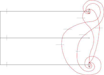
Figure 13: Generators of representatives of the $G$’s and $\bar{G}$’s, which partition the $Q_{3}$ and $Q_{3}$’s

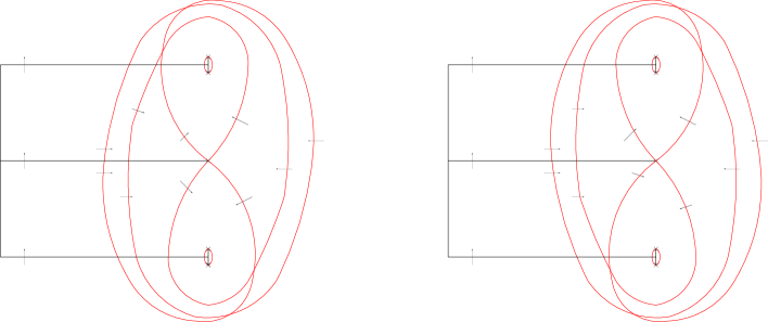
Figure 14: Sketch of the new curves needed to partition the extra states

There remains, of course, the curves which partition upper- and lower-barred $Q_{1}$ and $Q_{2}$’s, a simplified version of which we show pictorially in fig. (14). The regions around the two cores are devoid of lower-barred states, having a smaller spectrum than the weak coupling one. Remember that the $Q_{3}$’s and $\bar{Q}_{3}$’s in these regions are partitioned by $G$ and $\bar{G}$’s. This time we also need five copies in order to range over all $n$. All three quarks must be present throughout this region of the moduli space, including inside the cores. The fact that they should not pass through a core (other than their own) return and pass through again in the same direction alerts us to the fact that the situation is more complicated than we have drawn. Naturally curves involving, say, $Q_{1}$’s as constituent states, which arc around the $\alpha_{1}$ core will actually touch the core after wrapping around the requisite number of times (then crossing back through $N_{1}$ the same amount of times to return to the same global picture as fig. (14)). Thus a more accurate picture would be fig. (15), where we have drawn the intersections for a particular choice of $n$. Looking at the core in detail in fig. (16), where we have included just the states which transform to $\lambda_{2}$ and $\lambda_{3}$ through the quantum cut, we see how they cannot leave the core and come back in the other side. This allows for the existence of all the quarks in the core to be consistent. The presence of these further states is no problem.

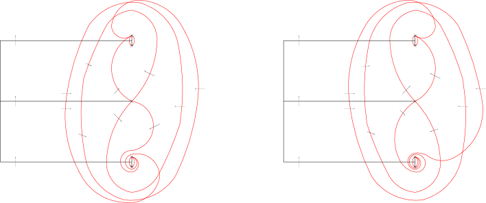
Figure 15: A more accurate depiction of fig. 14 for a particular $n$

The gauge bosons produced become unstable, as explained in [3], on curves encircling the cores. If we define $\bar{S}$’s in the same way as (2) but for $\bar{Q}$’s, then we have within one section of core only the states (fixed $n$, all $m$), $Q_{i}^{n},Q_{i}^{n+1},\bar{Q}_{i}^{n},\underline{Q}_{i}^{n+1},S_{m,\,i}^{n-1},S_{m,\,i}^{n},\bar{S}_{m,\,i}^{n-1},\bar{S}_{m,\,i}^{n}$ and the three quarks. A typical core is shown in fig. (17).

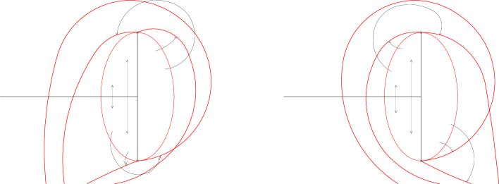
Figure 16: The consistency of extra states in the $\alpha_{1}$ core

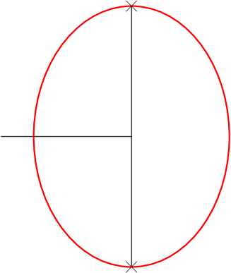
Figure 17: The states within the single core for one flavour, large $R/\Lambda$

Double cores, where they might begin to exist here, are also highly similar to the pure case. Additional curves surrounding them signal the place where the $\bar{S}$’s with large $m$, like their unbarred counterparts, are no longer stable. On each side of the branch cut $V$ we have four $S$’s, corresponding to them, four (of each flavour) $\bar{S}$’s, $N_{f}$ flavours of three quarks, as well as the two states which become massless in that region of that arm’s core connected to this side of $V$. An example can be found in fig. (18).

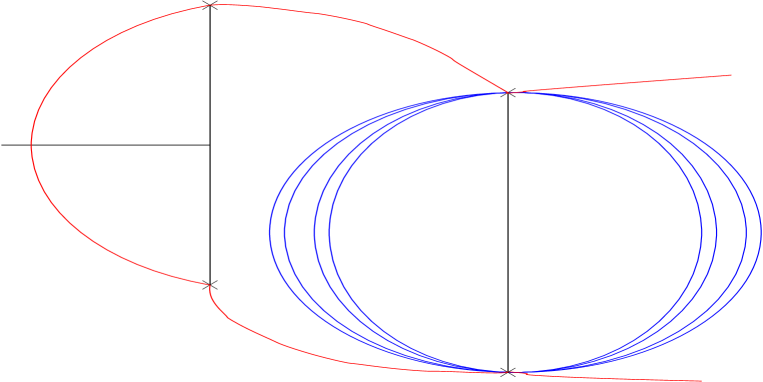
Figure 18: The states within the double core for one flavour

3.5 Larger $\Lambda$

Considering the moduli space at a fixed radius, we find there are three regimes, each more complex than the next. First, the infinite radius limit. Here the cuts and curves for all flavours with any bare masses are in identical positions. Shrinking $R$, but keeping $R\gg\Lambda$, $R\gg m_{i}$, we get models which are largely the same, the differences following a simple pattern, such as having a monodromy which acts, after three rotations, as $n\rightarrow n-(6-N_{f})$. They contain simple cores where one of the U$(1)$’s becomes strongly coupled. Finally, we get to $R\sim\Lambda$. Even for SU$(2)$ this is not formulaic, but almost every case needs to be treated individually, having its own accidental symmetries and other quirks.

For SU$(3)$, the job of pinning everything down exactly becomes unwieldy. We have limited our scope to just the generics. We can determine, for instance, how many double cores there will be, and roughly where they lie, for the massless and the equal bare mass cases. Except in the simplest examples, understanding exactly how the trefoliate curve degenerates into circles, and precisely the intermediate monodromies and states is a weighty challenge which we have not properly met. The one massless flavour example is a case in point: Its particular foible, as one can see from Table 3 in the Appendix, is that the quark singularity does not factor off as in the other massless cases, except in the large $R/\Lambda$ limit. For merely large $R/\Lambda$ we will see it in our three-spherical sections as portrayed above, a separate circular singularity. When $R\sim\Lambda$, however, it must merge with the remains of the other, what was trefoliate, curve. At a radius where this has begun to occur, from the perspective of our radial sections, this can only happen when the quark singularity and part of the old trefoil with exactly the same monodromy coincide, then disappear from view. We can thus deduce that the quark monodromy must pass through a core in order to become dyonic. This is what happens in general in SU$(2)$ to the singularity of a massive quark when we reduce $|m|$ to be very small.

In order to get to a position which does this, it is obvious that (as we shrink $R$) the quark singularity must (repeatedly) intersect the other curve before passing through it. From table 3, we can see that, if $v$ is roughly zero when this happens (the quark singularity only picks up corrections at order $(\Lambda^{5})^{3}$) then there are five intersections. This fills a faithful representation of the five-fold symmetry listed in Table 1. An example of where we believe this merging occurs is shown in fig. (19).

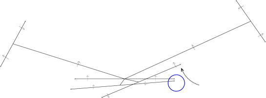
Figure 19: A place in the moduli space (ringed) where what was the quark singularity is equal and opposite, and nearly superposed with a dyonic singularity prior to merging.

If we continue to reduce $R/\Lambda$ we believe something akin to the quark singularity then re-emerges, we then get to a value (which can be read from Table 4 in the Appendix) where the trefoliate curve self-intersects and double cores arise, one at each of five points. In the singularity/core crossings too there will be, as there must, accumulation points, and some curves following into the core, joining these accumulation points to what begins as the quark singularity. These are a reduced set of those curves previously attached to the quark singularity, the rest the accumulation points restrict to end temporarily outside the core. Those inside involve only the states present within the core and their values after traversing the quark monodromy. Fig. (20) shows a sketch of this.

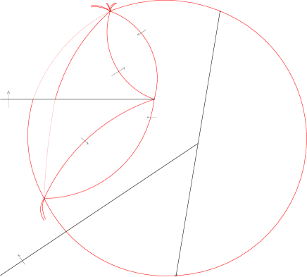
Figure 20: A quark singularity intersecting a single core. Note the formation of accumulation points and curves inwards from them. A $\bar{2}$ is any state with magnetic charge 2, etc.. There will be a curve for each.

If we add mass $|m|\ll\Lambda$ then we see little difference, even at $R\sim|m|$, as by the time we have shrunk $R\ll\Lambda$ the curve has disappeared anyway. For more flavours, we do see a qualitative difference, however. The quark singularity, which we can treat separately from the rest, keeps its integrity as a circle all the way down to $R=0$, but when we add mass it shrinks to a point before we reduce $R$ all the way.

4 More Flavours

We shall pick the case with three flavours (usually with nearly equal masses) to show how the previous argument generalises. Let us begin again with the simplest region at $R/\Lambda=\infty$. This time the quark monodromy becomes $[(0,\lambda_{3})_{100}][(0,\lambda_{3})_{010}][(0,\lambda_{3})_{001}]$, or $[\lambda^{a}_{3}][\lambda^{b}_{3}][\lambda^{c}_{3}]$ in simplified notation. The entire set of $Q_{3}$’s is invariant under this. It adds three upper bars to a $Q_{2}$ (cancelling with any lower ones), and adds three lower bars to the $Q_{1}$’s. Thus we see that $Q_{2}$ up to $\raisebox{2.0pt}{$\bar{\hskip 9.5pt}$}\raisebox{3.5pt}{$\bar{\hskip 9.5pt}$}\bar{Q}_{2}$ exist above the cut, and transform to $Q_{2}$ down to $Q\put(-9.5,-3.0){$\line(1,0){6.0}$}\put(-9.25,-2.0){$\line(1,0){6.0}$}\put(-9.0,-1.0){$\line(1,0){6.0}$}_{2}$ below. The reverse is true of the $Q_{1}$’s with the lower bars existing above the cut in the $3+$ region. Lower-barred $Q_{3}$’s do not exist anywhere, and all the upper-barred $Q_{3\pm}$’s exist in the same region as the pure ones.

If we restrict ourselves to large $R/\Lambda$, as already mentioned, the picture changes very little. The $G$ curves, which partition the $Q_{3}$’s, rotate to generate, not $\bar{G}$’s, but $\raisebox{2.0pt}{$\bar{\hskip 9.5pt}$}\raisebox{3.5pt}{$\bar{\hskip 9.5pt}$}\bar{G}$’s for three flavours, etc. , where all three bars persist on the component of the bound state not becoming massless. This is natural because, of course, in this sector only unbarred states become massless.

Now we need to find the curves which partition all the intermediate $Q_{3\pm}$’s as well as all the lower-barred and upper-barred $Q_{1}$’s in the $3+$(upper) and $3-$ regions respectively; and similarly, the lower-barred and upper-barred $Q_{2}$’s in $3+$(lower) and $3-$. These are just like the second batch of global curves described for one flavour. There are $N_{f}2^{N_{f}-1}$ copies of each of the two curves depicted in fig. (15). When all the bare masses are equal, the curves superpose. If not, they come in $N_{f}$ layers. Everywhere where a barred state becomes marginally stable to a pure state in the one flavour case, now a double barred will decay to the single barred one (outside it, if the masses differ); and a triple-barred one to the double, and so on up to $N_{f}$. Also in the one flavour case were places on these curves where a pure state would have the mass of a barred one plus a quark, for instance, $Q_{2}\rightarrow\bar{Q}_{2}+\lambda_{3}$. As the quark monodromy now changes states by $N_{f}$ bars, we find it becomes the second highest number of bars going to the highest, e.g.  for three flavours, equal masses, $\raisebox{2.0pt}{$\bar{\hskip 10.0pt}$}\bar{Q}_{2}\rightarrow\raisebox{2.0pt}{$\bar{\hskip 9.5pt}$}\raisebox{3.5pt}{$\bar{\hskip 9.5pt}$}\bar{Q}_{2}+\lambda_{3}$. Superposed are other curves we might think of as forming a chain

$$Q_{2}\rightarrow\lambda_{3}+\bar{Q}_{2}\rightarrow\lambda_{3}+\raisebox{2.0pt}{$\bar{\hskip 10.0pt}$}\bar{Q}_{2}\rightarrow\lambda_{3}+\raisebox{2.0pt}{$\bar{\hskip 9.5pt}$}\raisebox{3.5pt}{$\bar{\hskip 9.5pt}$}\bar{Q}_{2}.$$

We show one of the two curves in detail in fig. (21).

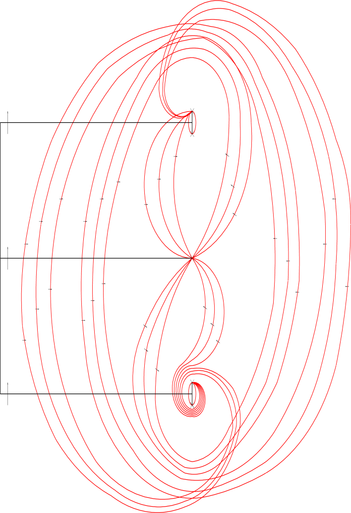
Figure 21: A look at one chain from one of the two sets of curves that help partition the three regions for $N_{f}=3$

When the masses are not equal then we have to take into account the s-charges. For three flavours, single barred states will have one index, equal to $a,b,$ or $c$, double bars will have two indices, which cannot be equal, and we can ignore these for triples which must have one of each. A typical equivalent of the previous chain would be

$$Q_{2}\rightarrow\lambda^{a}_{3}+\bar{Q}^{a}_{2}\rightarrow\lambda^{c}_{3}+\raisebox{2.0pt}{$\bar{\hskip 10.0pt}$}\bar{Q}^{ac}_{2}\rightarrow\lambda^{b}_{3}+\raisebox{2.0pt}{$\bar{\hskip 9.5pt}$}\raisebox{3.5pt}{$\bar{\hskip 9.5pt}$}\bar{Q}_{2}.$$

Including all six permutations of the indices gives 12 curves. Due to the symmetries, there will take 3 of each curve to cover all $n$. There would be another 36 such curves related to the second diagram in fig. (15). For $N_{f}=1$ to 5 we have $5,16,36,64$ and 80 examples respectively of each of the two types of curve.

A single core will contain the same states as the pure core plus whatever other states are left in that vicinity after all the previous curves have reduced the weak-coupling spectrum. We know this to be only the largest upper bars of the states not related to the core, e.g.  for the $\alpha_{1}$ core with three flavours, each region of the core contains $S_{m,1}^{n}$ for all $m$ and two consecutive $n$ (let us take $n=0,1$), as well as the same ${\raisebox{2.0pt}{$\bar{\hskip 9.5pt}$}\raisebox{3.5pt}{$\bar{\hskip 9.5pt}$}\bar{S}}_{m,1}^{n}$’s. It contains the quarks $\lambda_{i}^{a},\lambda_{i}^{b}$ and $\lambda_{i}^{c}$ for all three $i$. It also contains the maps of these through the quantum cut in the core, namely $\bar{Q}_{1}^{1}$ and $\underline{Q}_{1}^{2}$ for all s-charges. Finally, it contains the SU$(2)$ embeddings $Q_{1}^{1}$ and $Q_{1}^{2}$.

A double core, similarly, on the side touching the above single core will contain all ($N_{c}N_{f}=$) nine quarks, plus $Q_{1}^{1}$ and $Q_{1}^{2}$. Also $Q_{-2,\,1}^{-2}$ and $Q_{-2,\,1}^{-1}$, and $Q_{2,\,1}^{6}$ and $Q_{2,\,1}^{7}$; and the most upper-barred version of these last four, $\raisebox{2.0pt}{$\bar{\hskip 9.5pt}$}\raisebox{3.5pt}{$\bar{\hskip 9.5pt}$}\bar{Q}_{-2,\,1}^{-2},\,\raisebox{2.0pt}{$\bar{\hskip 9.5pt}$}\raisebox{3.5pt}{$\bar{\hskip 9.5pt}$}\bar{Q}_{-2,\,1}^{-1},\,\raisebox{2.0pt}{$\bar{\hskip 9.5pt}$}\raisebox{3.5pt}{$\bar{\hskip 9.5pt}$}\bar{Q}_{2,\,1}^{6}$, and $\raisebox{2.0pt}{$\bar{\hskip 9.5pt}$}\raisebox{3.5pt}{$\bar{\hskip 9.5pt}$}\bar{Q}_{2,\,1}^{7}$. (The dyons produced by the quarks traversing the quantum cut lose stability on curves lying between the accumulation points too).

To complete the picture, we show what happens when a quark singularity, e.g.  $[\lambda^{a}_{3}][\lambda^{b}_{3}][\lambda_{3}^{c}]$ crosses a double core region as above. The number of states remains the same, just the transformation that would have occurred had the complete double core and its adjoining single cores passed through the quark singularity is enacted by CMS’s connecting the singularity with accumulation points on the boundary of the core, sweeping across the intervening space. A sketch of this is shown in fig. (22). Note that although no intermediate barred states are stable in the core for equal masses (they are marginally stable on the sweeping CMS’s), when we perturb this situation a little by adding tiny mass differences and the quark singularity splits a little, such states can exist between the newly distinct sweeping curves.

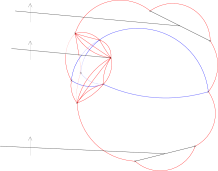
Figure 22: When a quark singularity intersects a double core. The two groups of three leaf-shaped curves signal the boundary of stability for the states that have come through the cut in either direction, as for the single core.

5 Flows Between the Examples

As a further consistency check, as well as exploring an important part of the parameter space, we should consider how, at least for large $R/\Lambda$ the models with a greater number of flavours flow into those with less as we take some of the $|m_{i}|$ to infinity, causing them to decouple from the effective theory. For simplicity we shall consider all the masses we take to infinity to be equal, and also all those left behind equal.

If we begin with both sets of equal masses the same, we have a quark singularity of order $N_{f}$. It is just the $N_{f}$-fold product $[\lambda_{3}^{a}][\lambda_{3}^{b}]...$. If we give extra (equal, here) mass to $N_{1}$ of them, then this singularity simply splits into the appropriate combinations of $N_{1}$ and $N_{f}-N_{1}$ of them. The singularity corresponding to the quarks with larger $|m_{i}|$ will be closer to the origin, as this will shrink to a point and disappear before the other one. All the curves which touched the singularity before it split had a $\lambda_{3}^{i}$ as a constituent of the marginal bound state. These curves will bifurcate, diverging from superposition to follow whichever of the two singularities contains the $\lambda_{3}$ with their s-charge label. At a fixed value of $R$ and $\Lambda$, $R\gg\Lambda$, increasing the bigger mass will see the corresponding quark singularity move ever closer to the origin. At a certain mass, it will have to pass through the core. This marks the transition from a space which looks largely like the $N_{f}$ moduli space, with small areas different, to one which looks largely like the $N_{f}-N_{1}$ space with a few isolated pockets of $N_{f}$-ness remaining, which shrink away as the mass increases further. As can be seen from fig. (23), before we reach that stage, the states which exist between the singularities transform nicely across the monodromy of the remaining fixed mass quarks.

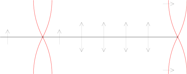
Figure 23: The reduced spectrum left between the two quark singularities consists of only those states that would be present for the lower, right-hand set, plus $\alpha_{3}$ states invariant under all the $[\lambda_{3}]$’s. Here we pick $N_{f}=3$ with two large masses.

As the divergent mass becomes larger, so too will the areas bound by curves which pass through its quark singularity. Inside these, the space carries only the smaller $N_{f}-N_{1}$ spectrum. If we extend our usual radial section to include the diametrically opposite half-plane too, as in fig. (24), we see that eventually the curves on both sides pass through infinity on our stereographic projection of the three-sphere. Continuing further, they restrict more and more of the space to be $N_{f}-N_{1}$, and act as the boundary confining the $N_{f}$ region inside a central sphere and an annulus each touching the circle that is the heavier quark singularity. After this circle touches the core, the annulus detaches and then both it and the sphere shrink away to nothing at a finite value of $|m|$ dependent on $R$ and $\Lambda$. Any states of the highest $N_{f}$ bars, formerly inside both sets of curves, will decouple as their mass tends to infinity.

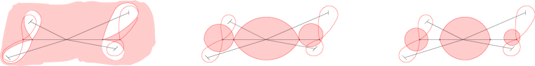
Figure 24: The shaded region represents the area where $\alpha_{1}$ and $\alpha_{2}$ magnetically charged dyons form bound states with the quarks which have the bare mass we take to infinity. There are 3 regimes: first the curves grow, then, when the quark singularity crosses the core, they merge at infinity, recombining to bound two regions. Finally, these split and shrink away.

The one flavour case is not so special if we now consider how, for $R\gg\Lambda$, the number of twists that the core undergoes changes by $N_{1}$ half-twists. As we increase the mass, in all cases in this regime, the first time the singularity surface intersects is when the $N_{1}$-fold quark singularity crosses the trefoliate curve with $N_{f}$ half-twists. This singularity is a separate curve from the trefoil if and only if $N_{1}\geq 2$. This could be seen to be the consequence of a Higgs branch being incident at this singularity, or just that such a multiple singularity cannot be equal to any of the single ones of the trefoliate curve. In any case, if we always let $N_{1}=1$, decoupling one flavour at a time, then the quark singularity must always merge with the other one. If we do this many times, we could alternatively have decoupled all at once. Thus we can tell that we must see ‘demerging’ too - the circle must reform on the other side of the trefoliate curve. Each merger-demerger has the effect of reducing the number of half-twists of the trefoliate curve by one. We believe this may occur as in fig. (25). When a double, or stronger, quark singularity passes through a core, we believe the two branches of the trefoliate curve simply intersect, before, during or after, to unwind the required number of times.

Figure 25: The outer curve represents the quark singularity, the inner one the trefoliate curve. In the second figure they merge in two places. The curve loses a half-twist and then they demerge.

The interested reader may have realized that in the other sectors of the moduli space, where $\alpha_{3}$ is not the non-simple root, the monodromies for the third root are different, and moreover depend on the number of flavours. In each case we have not $N_{3-}=[Q_{3-}^{n}][Q_{3-}^{n-1}]$, but the most upper-barred equivalent, e.g.  $\raisebox{2.0pt}{$\bar{\hskip 9.5pt}$}\raisebox{3.5pt}{$\bar{\hskip 9.5pt}$}\bar{N}_{3-}=[\raisebox{2.0pt}{$\bar{\hskip 9.5pt}$}\raisebox{3.5pt}{$\bar{\hskip 9.5pt}$}\bar{Q}_{3-}^{n}][\raisebox{2.0pt}{$\bar{\hskip 9.5pt}$}\raisebox{3.5pt}{$\bar{\hskip 9.5pt}$}\bar{Q}_{3-}^{n-1}]$. The only way to enforce a change at the transition is to sweep around this third of the trefoil with the departing quark monodromy, in much the same way as in [6] for SU$(2)$. We show this in diagrammatic form in fig. (26). Our ability to do this is based on the group relation

$$\bar{N}_{3-}=[\lambda_{2}]^{-1}N_{3-}[\lambda_{2}]=[\lambda_{1}]N_{3-}[\lambda_{1}]^{-1}$$

which also holds if we put an extra bar on all the $N_{3}$’s, any number of times.

Figure 26: How the cut of the singularity of quarks with bare mass tending to infinity loops around the third arm (to which we have paid little attention so far) before shrinking. $R$ increases to the right.

The introduction of bare masses changes the position of all the multiple points of the singularity curve. The first intersections, just described, move outwards such that when we reach the regime $m\gg\Lambda$, $m={\rm Max}\,|m_{i}|$, they occur at scale $R\sim m$. All the others vary with smaller powers of $m$, none remaining fixed. One could think of this as marking a steady transition from dependence on $\Lambda_{N_{f}}$ through to $\Lambda_{N_{f}-N_{1}}=(m_{1}\dots m_{N_{1}}\Lambda_{N_{f}}^{6-N_{f}})^{1/(6-N_{f}+N_{1})}$. We cannot describe in detail the tangled webs which ensue, but merely point out that when we add masses, the multiple intersections tend to split, and all the discrete symmetry of the model is lost as the positions of the intersections move towards those of the theory with a lower number of flavours. Upon taking these masses to infinity, these intersection points merge with others to form higher order intersections again.

6 Conclusions

We have thus described qualitatively, in some, but not complete detail, a consistent model of low-energy effective ${\cal N}=2$ supersymmetric gauge theory for SU$(3)$ with up to 5 flavours of hypermultiplets in the fundamental. We have concentrated on the regime where $R\gg\Lambda_{N_{f}}$ and listed the BPS spectra which occur here. Just as we found for the pure case, there are mutually disjoint areas in the weak-coupling limit carrying different BPS spectra. In each of these there exist $3=N_{c}(N_{c}-1)/2$ infinite towers of stable BPS dyons. We have further $3N_{f}$ quarks, and $2^{N_{f}}$ possible bound states of these with each element of each of the three towers. In a particular region, it may instead be energetically favourable for one of the towers to bind with antiquarks.

There are always single cores — areas where one of the remnant U$(1)$’s is strongly coupled. There is also an area where some of the quarks (one of the elements of the colour triplet for each flavour) become light. There are then regions which strictly include the core, and some of the latter area, in which most of these dyon-quark bound states either lose stability, or, interestingly, bind further with more quarks, until they have one of each flavour and so become a flavour singlet. This state of affairs persists in the core, where the bound states occur only with the reduced number of those dyons which exist there in the pure model.

We have additional, and rather complicated singularity structure to that of the pure case. For fixed large $R/\Lambda$ we see a ‘trefoliate’ curve which twists about a trefoil, and a circular ‘quark singularity’ curve for each flavour, coincident for those flavours which possess the same bare mass. At least for when we have some large masses, we can be sure that these two intersect before other self-intersections complicate the picture. Then the quark singularity must pass through the single core. Double cores also exist, at the intersection of single ones. We are then led to the question of whether the quark singularity passes through these.

We have also tweaked the model we presented for the pure case [3]. The addition of curves upon which higher spin multiplets become unstable accommodates the conventional weak coupling spectrum, without needing to invoke the existence of as many of these states co-existing with simple root magnetic charge. Despite impressive machinery [14], the existence of these states has yet to be disproved, so we offer this model as an (more likely) alternative rather than a correction. Within the double core, the use of an extra branch cut does seem a correction, allowing us a smaller, more symmetric BPS spectrum, which transforms more clearly as the quantum monodromies pass through each other. We think a model along the lines of [3] would still be possible, but it becomes almost intractably messy.

Based on [15], in [16, 8] Dorey et al.  argued that at a particular point of the SU$(N_{c})$ moduli space with matter the massive BPS spectrum is equivalent to a particular two-dimensional $(2,2)$-SUSY gauge theory with U$(N_{c})$ flavour symmetry. In one regime, the corresponding point in Seiberg-Witten is at weak-coupling. However, the 2D theory has a limit with a dual description and a different, smaller, calculable BPS spectrum corresponding to when our point is at strong coupling with a reduced set of stable states. There is scope, then, for our predictions to be matched against each other.

Thus far we have given the impression that the quark singularities are coincident if and only if the bare masses of all the flavours are the same. This is not quite true. When $N_{f}\geq N_{c}$ there is one other possibility, which occurs when the auxiliary curve degenerates into two equal factors. For SU$(3)$ with three flavours this occurs when the masses $m_{i}$ are the three roots of $m_{i}^{3}-um_{i}+v=0$. Necessarily they sum to zero. So for each $u,\,v$ we could find masses such that all the quark singularities (or whatever they have become at strong coupling) are coincident, and the auxiliary curve a square. Alternatively, for each set of $m_{i}$ summing to zero, we could find the $u,\,v$ coordinates of where such a singularity would occur. For four and five flavours, this class falls into the set of occurrences for which three singularities are coincident (the others coincident too as special cases). The Galois group of the defining equations treats three, say $m_{1},\,m_{2},\,m_{3}$, differently to the other one or two. The theme linking these events is that in each case these ${}^{N_{f}}C_{3}$ order 3 singularities are also the root of a baryonic Higgs branch.

Although we offer no proof of the fact, we expect the theories of three equal masses and of those at the root of this baryonic branch to be very similar. For SU$(2)$, where the relations for two flavours to be at this root are $m_{1}=-m_{2}=m$, and $u=m^{2}-\Lambda^{2}/8$, as opposed to $m_{1}=m_{2}$ and $u=m^{2}+\Lambda^{2}/8$. If, for the former, we let $m\rightarrow im$, we get the mirror image moduli space, the only difference we find between whether $m_{2}=\pm m_{1}$ is that of the natural assignment of s-charges. For SU$(3)$, we find only a slight discrepancy: the values of $u$ and $v$ for three equal masses are given implicitly as those which solve $m^{3}-um+v=k(\Lambda_{N_{f}})$ where $k(\Lambda_{3})=\Lambda_{3}^{3}/4$, $k(\Lambda_{4})=m\Lambda_{4}^{2}/2$ and $k(\Lambda_{5})=m^{2}\Lambda_{5}/4$. The authors of [8] argue that the baryonic Higgs branch has a strong-coupling region with only a finite spectrum. For us this implies that for three or more flavours, the quark singularity must pass through a double core. We cannot definitively say whether or not this is true, but it seems a perfectly reasonable assumption. Given this, we agree on both weak and strong coupling spectra, with possible differences in that in almost all cases we have the intermediately barred states only at most marginally stable in the neighbourhood of the singularity, and also that we have included regions in this neighbourhood where bound states with the antiquarks, rather than with the quarks exist. Thus modulo these slight discrepancies, we find ourselves to be in broad agreement, lending weight to both arguments.

Finally we should state that it would be fascinating to extend this analysis to the case of six flavours where other studies exist [27, 28]. There are also string web constructions and other methods involving the solution of geodesic equations, such as [29, 30, 31, 32, 19] which could in principle reproduce these results. We would like, eventually, to write $a$ and $a_{D}$ as ratios of two-variable theta functions and then to plot the positions of the CMS’s exactly. This is very much more involved than for SU$(2)$ where the underlying mathematical structure is well documented.

Appendix A Singularity Curves

We choose to use the auxiliary curves of [22], in Table 2 we list first the massless cases, then those of general mass.

$N_{f}$	$y^{2}=$
$0$	$(x^{3}-ux-v)^{2}-\Lambda^{6}_{0}$
$1$	$(x^{3}-ux-v)^{2}-\Lambda^{5}_{1}x$
$2$	$(x^{3}-ux-v)^{2}-\Lambda^{4}_{2}x^{2}$
$3$	$(x^{3}-ux-v+\Lambda_{3}^{3}/4)^{2}-\Lambda^{3}_{3}x^{3}$
$4$	$(x^{3}-ux-v+\Lambda_{4}^{2}x/4)^{2}-\Lambda^{2}_{4}x^{4}$
$5$	$(x^{3}-ux-v+\Lambda_{5}x^{2}/4)^{2}-\Lambda_{5}x^{5}$
$1m$	$(x^{3}-ux-v)^{2}-\Lambda^{5}_{1}(x+m_{1})$
$2m$	$(x^{3}-ux-v)^{2}-\Lambda^{4}_{2}(x+m_{1})(x+m_{2})$
$3m$	$(x^{3}-ux-v+\Lambda_{3}^{3}/4)^{2}-\Lambda^{3}_{3}(x+m_{1})(x+m_{2})(x+m_{3})$
$4m$	$(x^{3}-ux-v+\Lambda_{4}^{2}(x+m_{1}+m_{2}+m_{3}+m_{4})/4)^{2}-\Lambda^{2}_{4}(x+m_{1})(x+m_{2})(x+m_{3})(x+m_{4})$
$5m$	$(x^{3}-ux-v+\Lambda_{5}(x^{2}+(m_{1}+m_{2}+m_{3}+m_{4}+m_{5})x+(m_{1}m_{2}+m_{1}m_{3}+\dots+m_{4}m_{5}))/4)^{2}$
	$-\Lambda_{5}(x+m_{1})(x+m_{2})(x+m_{3})(x+m_{4})(x+m_{5})$

Table 2: A list of the auxiliary elliptic curves for massless, then general masses

The singularities of each curve are the set of $u$ and $v$ where the elliptic curve degenerates, i.e.  has some roots in common. This can be written as the zero set of a polynomial, the discriminant. In Table 3 we write this for massless flavours.

$N_{f}$	Discriminant
$0$	$\Lambda^{18}(4u^{3}-27(v+\Lambda^{3})^{2})(4u^{3}-27(v-\Lambda^{3})^{2})$
$1$	$\Lambda^{15}(3125\Lambda^{15}-256\Lambda^{5}u^{5}-22500\Lambda^{10}uv+1024u^{6}v+43200\Lambda^{5}u^{2}v^{2}-13824u^{3}v^{3}+46656v^{5})$
$2$	$-64\Lambda^{12}v^{2}(4\Lambda^{6}+12\Lambda^{4}u+12\Lambda^{2}u^{2}+4u^{3}-27v^{2})(4\Lambda^{6}-12\Lambda^{4}u+12\Lambda^{2}u^{2}-4u^{3}+27v^{2})$
$3$	$\frac{1}{16}\Lambda^{9}(\Lambda^{3}-4v)^{3}(729\Lambda^{6}u^{3}-256u^{6}-3888\Lambda^{3}u^{3}v+3456u^{3}v^{2}+2916\Lambda^{3}v^{3}-11664v^{4})$
$4$	$4\Lambda^{6}v^{4}(-\Lambda^{2}u+8\Lambda^{2}u^{2}-16u^{3}+2\Lambda^{3}v-72\Lambda uv+108v^{2})$
	$(-\Lambda^{2}u+8\Lambda^{2}u^{2}-16u^{3}-2\Lambda^{3}v+72\Lambda uv+108v^{2})$
$5$	$4\Lambda^{3}v^{5}(-\Lambda^{2}u^{5}+256u^{6}-2\Lambda^{3}u^{3}v+528\Lambda u^{4}v-\Lambda^{4}uv^{2}+300\Lambda^{2}u^{2}v^{2}$
	$-3456u^{3}v^{2}-4\Lambda^{3}v^{3}+4212\Lambda uv^{3}+11664v^{4})$

Table 3: The discriminants for massless flavours

$N_{f}$	fac${}^{\rm\underline{n}}$	sing facs	class	$u$	$v$	$R$
$0$	$AB$	$AB$	$*M^{2}_{2}$	$3\Lambda^{2}/\sqrt[3]{4}$	$0$	$27$
		$A^{2},B^{2}$	$*M^{0}_{3}$	$0$	$\pm\Lambda^{2}$	$27$
$1$	$A$	$A^{2}$	$M^{1}_{0}$	$5\Lambda^{2}\sqrt[5]{3/2^{12}}$	$5\Lambda^{3}/\sqrt[5]{2^{13}3^{6}},\,(uv$	$25\sqrt[5]{2^{-21}3^{8}}$
		$A^{2}$	$M^{1}_{0}$	$-5\Lambda^{2}/\sqrt[5]{2^{8}3}$	$-5\Lambda^{3}/\sqrt[5]{2^{2}3^{9}},\in\mathbb{R})$	$25\sqrt[5]{2^{-14}3^{7}}$
$2$	$Q^{2}AB$	$Q^{2}A^{2},Q^{2}B^{2}$	$*M^{2}_{4}$	$\pm\Lambda^{2}$	$0$	$4$
		$AB$	$M^{2}_{0}$	$\pm i\Lambda^{2}/\sqrt{3}$	$\sqrt{\pm 32i/81\sqrt{3}}$	$1/\sqrt{3}$
$3$	$Q^{3}A$	$Q^{3}A$	$M^{3}_{2}$	$0$	$\Lambda^{3}/4$	$27/16$
		$Q^{3}A$	$M^{3}_{2}$	$-3\Lambda^{2}/\sqrt[3]{2^{8}}$	$\Lambda^{3}/4$	$3^{3}5/64$
		$A^{3}$	$M^{3}_{0}$	$-3^{2}\Lambda^{2}/\sqrt[3]{2^{12}}$	$9\Lambda^{3}/32$	$3^{6}/2^{8}$
$4$	$Q^{4}AB$	$Q^{4}AB$	$M^{4}_{2}$	$0$	$0$	$0$
		$Q^{4}AB$	$*M^{4}_{4}$	$\Lambda^{2}/4$	$0$	$1/16$
		$AB$	$M^{4}_{0}$	$\Lambda^{2}/36$	$2\Lambda^{3}/\sqrt{3^{9}}$	$65/3^{6}2^{4}$
		$A^{2},B^{2}$	$M^{4}_{0}$	$\Lambda^{2}/12$	$\mp\Lambda^{3}/27$	$17/27$
$5$	$Q^{5}A$	$Q^{5}A^{3}$	$M^{5}_{4}$	$0$	$0$	$0$
		$Q^{5}A$	$M^{5}_{2}$	$\Lambda^{2}/2^{8}$	$0$	$1/2^{22}$
		$A^{2}$	$M^{5}_{0}$	$\frac{39\pm 55\sqrt{33}}{2^{13}3^{2}}\Lambda^{2}$	$\frac{2879\mp 561\sqrt{33}}{2^{18}3^{3}}\Lambda^{3}$	$\sim 5.1\times 10^{-7}$
						$2.0\times 10^{-5}$
		$A^{2}$	$M^{5}_{0}$	$\Lambda^{2}/3^{5}$	$-\Lambda^{3}/2^{13}3^{2}$	$5045113/2^{16}3^{15}$

Table 4: Intersection points of the singularity curves for massless matter.

The main features of the discriminants are how they factorize, and their self-intersections, or multiple zeroes. In Tables 4 and $5$ we note the position and order of most of them (for equal masses). We do not claim this to be comprehensive and exhaustive, except for zero masses, but based purely on those that could readily be open to solution by radicals using Mathematica and expressible in a small space. The first column denotes which example we are considering, e.g., $4m2$ is four flavours, two of which are massive with equal mass $m$. In the second, we state the number of factors, by labelling each quark singularity as $Q$, and each other factor with a capital letter $A,B,\dots$. In the third column is a word where we include one occurrence of each factor for each order of zero that factor has at the singularity. The number of these gives the order of the singularity, i.e.  the first order of derivatives where any one of which has a non-zero value at the singularity. It is useful to distinguish these singularities by the universality class of the superconformal field theory which exists there, as defined in [33], so we state this in column four. We add a star if this is not of the trivial class 1 in [33]. Columns five and six state, where possible, the ($u,v$) positions of the singularity, and the last column, the sixth power of the radius in units of $\Lambda$, i.e.  $(4|u|^{3}+27|v|^{2})/\Lambda^{6}$. Note that where square and cube roots, etc., are given as coordinates, we imply that there is one of these roots at each of the possible values.

$N_{f}$	fac${}^{\rm\underline{n}}$	sing facs	ord	$u$	$v$
$2m2$	$Q^{2}AB$	$Q^{2}A,Q^{2}B$	$3$	$3m^{2}\pm\Lambda^{2}$	$m(2m^{2}\pm\Lambda^{2})$
		$Q^{2}A,Q^{2}B$	$3$	$(3m^{2}\pm 4\Lambda^{2})/4$	$m(\pm\Lambda^{2}-m^{2}/4)$
		$A^{2},B^{2}$	$2$	$\pm\Lambda^{2}$	$\pm\Lambda^{2}m$
		$AB$	$2$	4 points
$3m1$	$Q^{2}A$	$Q^{2}A$	$3$	$\sqrt{\Lambda^{3}m}$	$\Lambda^{3}/4$
		$Q^{2}A$	$3$	3 points	$\Lambda^{3}/4$
$3m2$	$Q^{2}A$	$Q^{2}A$	$2$	$3m^{2}\pm i\sqrt{\Lambda^{3}m}$	$\frac{\Lambda^{3}+8m^{3}+4mi\sqrt{\Lambda^{3}m}}{4}$
		$Q^{2}A$	$3$	3 points
$3m3$	$Q^{3}A$	$Q^{3}A$	$4$	$3m^{2}$	$(\Lambda^{3}+8m^{3})/4$
		$Q^{3}A$	$4$	3 points
$4m1$	$Q^{3}A$	$Q^{3}A$	$4$	$\Lambda^{2}/4$	$\Lambda^{2}m/4$
		$Q^{3}A$	$4$	4 points	$\Lambda^{2}m/4$
$4m2$	$Q_{1}^{2}Q_{2}^{2}AB$	$Q_{1}^{2}Q_{2}^{2}$	$4$	$(\Lambda^{2}+4m^{2})/4$	$\Lambda^{2}m/2$
		$Q_{1}^{2}A,Q_{1}^{2}B$	$3$	$(\pm 3m^{2}-2\Lambda m)4$	$\frac{\Lambda m(\Lambda\mbox{-}2m)+m^{3}(\pm 3\mbox{-}4)}{4}$
		$Q_{1}^{2}A,Q_{1}^{2}B$	$3$	$(\Lambda^{2}\pm 4\Lambda m+12m^{2})/4$	$\frac{2\Lambda^{2}m\pm\Lambda m^{2}+8m^{3}}{4}$
		$Q_{2}^{2}A,Q_{2}^{2}B$	$3$	$(\Lambda^{2}\pm 4\Lambda m)/4$	$\Lambda^{2}m/2$
		$Q_{2}^{2}A,Q_{2}^{2}B$	$3$	$\pm\Lambda m$	$\Lambda^{2}m/2$
		$A^{2},B^{2}$	$2$	$-(\Lambda^{2}\pm 12\Lambda m)/4$	$(27m\pm 2\Lambda)/54$
		$AB$	$2$	5 points
$4m3$	$Q^{3}A$	$Q^{3}A$	$4$	$(\Lambda^{2}+12m^{2})/4$	$\frac{27m\pm 2\Lambda}{54}\Lambda^{2}$
		$Q^{3}A$	$4$	4 points
$4m4$	$Q^{4}AB$	$Q^{4}AB$	$6$	$(\Lambda^{2}+12m^{2})/4$	$m(\Lambda^{2}+2m^{2})$
		$Q^{4}A,Q^{4}B$	$5$	$\frac{3m}{4}(2\Lambda\pm m)$	$\frac{3\Lambda^{2}m+6\Lambda m^{2}-(4\mp 3)}{4}$
		$AB$	$2$	$(\Lambda^{2}+12m^{2})/4$	$\frac{\Lambda^{2}m(\Lambda+7m)(2\Lambda+19m)}{12\Lambda^{2}+27\Lambda m+27m^{2}}$
		$A^{2},B^{2}$	$2$	$-(\pm\Lambda^{2}+24\Lambda m)/12$	$\frac{\Lambda}{27}(\Lambda^{2}\pm 27\Lambda m-27m^{2})$
		$AB$	$2$	3points
$5m1$	$Q^{4}A$	$Q^{4}A^{2}$	$6$	$\Lambda m/4$	$0$
		$Q^{4}A^{2}$	$6$	$0$	$0$
		$Q^{4}A$	$5$	$(\Lambda+16m)^{2}/2^{8}$	$0$
$5m2$	$Q_{1}^{2}Q_{2}^{3}A$	$Q_{1}^{2}A$	$3$	$3m^{2}\pm i\sqrt{\Lambda m^{3}}$	$2m^{2}\Lambda\pm im\sqrt{m^{3}\Lambda}$
		$Q_{1}^{2}$	$3$	$\frac{\Lambda^{2}+48\Lambda m+384m^{2}\pm\sqrt{\Lambda(\Lambda+32m)^{3}}}{2^{9}}$	$m(u-m^{2})$
		$Q_{2}^{3}A$	$5$	$m^{2}+\Lambda m/4$	$\Lambda m^{2}/4$
		$Q_{2}^{3}A$	$4$	$\Lambda m/2$	$\Lambda m^{2}/4$
		$Q_{2}^{3}A$	$4$	3 points	$\Lambda m^{2}/4$

$N_{f}$	fac${}^{\rm\underline{n}}$	sing facs	ord	$u$	$v$
$5m3$	$Q_{1}^{3}Q_{2}^{2}A$	$Q_{1}^{3}A$	$4$	$(\Lambda m+12m^{2})/4$	$(2m^{2}\Lambda+8m^{3})/4$
		$Q_{1}^{3}A$	$4$	3 points
		$Q_{1}^{3}Q_{2}^{2}$	$5$	$(11\Lambda m+4m^{2})/4$	$3\Lambda m^{2}/4$
		$Q_{2}^{2}A$	$3$	$(3\Lambda m\pm 4\sqrt{\Lambda m^{3}})/4$	$3\Lambda m^{2}/4$
		$Q_{2}^{2}A$	$3$	$\frac{\Lambda(\Lambda+96m)\pm\sqrt{(\Lambda+96m)^{3}}}{2^{9}}$	$3\Lambda m^{2}/4$
$5m4$	$Q^{4}A$	$Q^{4}A$	$5$	$(\Lambda m+6m^{2})/2$	$(5\Lambda m^{2}+8m^{3})/4$
		$Q^{4}A$	$5$	3 points
$5m5$	$Q^{5}A$	$Q^{5}A$	$6$	$(3\Lambda m+12m^{2})/4$	$(9\Lambda m^{2}+8m^{3})/4$
		$Q^{5}A$	$6$	$\frac{\Lambda^{2}+144\Lambda m+384m^{2}\pm\sqrt{\Lambda(\Lambda+96m)^{3}}}{2^{9}}$	$(3\Lambda m-2m^{3}+2mu)/2$

References

- [1] N. Seiberg and E. Witten, “Electric-Magnetic Duality, Monopole Condensation, And Confinement In N=2 Supersymmetric Yang-Mills Theory”, Nucl. Phys. B 426 (1994) 19.
- [2] N. Seiberg and E. Witten, “Monopoles, Duality and Chiral Symmetry Breaking in N=2 Supersymmetric QCD”, hep-th/9408099, Nucl. Phys. B 431 (1994) 484-550.
- [3] B. J. Taylor, “On The Strong-Coupling Spectrum of Pure SU Seiberg-Witten Theory”, hep-th/0107016 J. High Energy Phys. 08 (2001) 031.
- [4] A. Bilal, F. Ferrari, “The Strong-Coupling Spectrum of the Seiberg-Witten Theory”, hep-th/9602082, Nucl. Phys. B 469 (1996) 387.
- [5] A. Bilal, F. Ferrari, “Curves of Marginal Stability and Weak and Strong-Coupling BPS Spectra in Supersymmetric QCD”, hep-th/9605101, Phys. Lett. B 480 (1996) 589.
- [6] A. Bilal, F. Ferrari, “The BPS Spectra and Superconformal Points in Massive N=2 Supersymmetric QCD”, hep-th/9706145 Nucl. Phys. B 516 (1998) 175.
- [7] F. Ferrari, “The dyon spectra of finite gauge theories”, hep-th/9702166, Nucl. Phys. B 501 (1997) 53-96.
- [8] N. Dorey, T. Hollowood, D. Tong, “The BPS Spectra of Gauge Theories in Two and Four Dimensions”, hep-th/9902134, J. High Energy Phys. 05 (1999) 006.
- [9] T. Hollowood, C. Fraser, “On the weak coupling spectrum of N=2 supersymmetric SU(n) gauge theory”, hep-th/9610142, Nucl. Phys. B 490 (1997) 217-238.
- [10] A. Klemm, W. Lerche, S. Theisen, S. Yankielowicz, “Simple Singularities and N=2 Supersymmetric Yang-Mills Theory”, hep-th/9411048, Phys. Lett. B 344 (1995) 169-175.
- [11] A. Klemm, W. Lerche, S. Theisen, S. Yankielowicz, “On the Monodromies of N=2 Supersymmetric Yang-Mills Theory”, hep-th/9412158.
- [12] J. Gauntlett, N. Kim, J. Park, P. Yi,“Monopole Dynamics and BPS Dyons N=2 Super-Yang-Mills Theories”, hep-th/9912082, Phys. Rev. D 61 (2000) 125012.
- [13] J. Gauntlett, C. Kim, K. Lee, P. Yi, “General Low Energy Dynamics of Supersymmetric Monopoles”, hep-th/0008031, Phys. Rev. D 63 (2001) 065020.
- [14] M. Stern, P. Yi, “Counting Yang-Mills Dyons with Index Theorems”, hep-th/0005275, Phys. Rev. D 62 (2000) 125006.
- [15] A. Hanany and K. Hori, “Branes and N=2 Theories in Two Dimensions” hep-th/9707192, Nucl. Phys. B 513 (1998) 119.
- [16] N. Dorey. “The BPS Spectra of Two-Dimensional Supersymmetric Gauge Theories with Twisted Mass Terms”, hep-th/9806056, J. High Energy Phys. 11 (1998) 005.
- [17] T. Hollowood, “Dyon electric charge and fermion fractionalization”, hep-th/9705041, Nucl. Phys. B 517 (1998) 161-178.
- [18] T. Hollowood, “Semi-Classical Decay of Monopoles in N=2 Gauge Theory”, hep-th/9611106.
- [19] M. Henningson, P. Yi “Four-dimensional BPS-spectra via M-theory”, hep-th/9707251, Phys.Rev. Phys. Rev. D 57 (1998) 1291.
- [20] A. Klemm, W. Lerche, S. Theisen, “Nonperturbative Effective Actions of N=2 Supersymmetric Gauge Theories”, hep-th/9505150, Int. J. Mod. Phys. A 11 (1996) 1929-1974.
- [21] P. Argyres, M. Douglas, “New Phenomena in SU(3) Supersymmetric Gauge Theory”, hep-th/9505062, Nucl. Phys. B 448 (1995) 93-126.
- [22] A. Hanany, Y. Oz, “On the Quantum Moduli Space of Vacua of Supersymmetric Gauge Theories”, hep-th/9505075, Nucl. Phys. B 452 (1995) 283-312.
- [23] A. Brandhuber, K. Landsteiner, “On the Monodromies of N=2 Supersymmetric Yang-Mills Theory with Gauge Group SO(2n)”, hep-th/9507008, Phys. Lett. B 358 (1995) 73-80.
- [24] U. H. Danielsson, B. Sundborg, “The Moduli Space and Monodromies of N=2 Supersymmetric Yang-Mills Theory”, hep-th/9504102, Phys. Lett. B 358 (1995) 273-280.
- [25] F. Ferrari, “Charge fractionization in N=2 supersymmetric QCD”, hep-th/9609101, Phys. Rev. Lett. 78 (1997) 795-798.
- [26] K. Lee, E. Weinberg, P. Yi, “The Moduli Space of Many BPS Monopoles for Arbitrary Gauge Groups”, hep-th/9602167, Phys. Rev. D 54 (1996) 1633-1643.
- [27] P. Argyres, A. Buchel, “The Nonperturbative Gauge Coupling of N=2 Supersymmetric Theories”, hep-th/9806234, Phys. Lett. B 442 (1998) 180-184.
- [28] P. Argyres, A. Buchel, “Deriving N=2 S-dualities from Scaling for Product Gauge Groups”, hep-th/9804007, Phys. Lett. B 431 (1998) 317-328.
- [29] A. Brandhuber, S. Stieberger, “Self-Dual Strings and Stability of BPS States in N=2 SU(2) Gauge Theories”, hep-th/9610053, Nucl. Phys. B 488 (1997) 199-222.
- [30] J. Schulze, N. Warner, “BPS Geodesics in N=2 Supersymmetric Yang-Mills Theory”, hep-th/9702012, Nucl. Phys. B 498 (1997) 101-118.
- [31] A. Mikhailov, N. Nekrasov, S. Sethi, “Geometric Realizations of BPS States in N=2 Theories”, hep-th/9803142, Nucl. Phys. B 531 (1998) 345-362.
- [32] O. Bergman, A. Fayyazuddin, “String Junctions and BPS States in Seiberg-Witten Theory”, hep-th/9802033, Nucl. Phys. B 531 (1998) 108-124.
- [33] T. Eguchi, K. Hori, K. Ito, S.-K. Yang, “Study of Superconformal Field Theories in Dimensions”, hep-th/9603002, Nucl. Phys. B 471 (1996) 430-444.