The clash between de Sitter
and anti-de Sitter space

Abstract:

We investigate solutions that are dynamically evolving between asymptotically de Sitter and asymptotically anti-de Sitter regions in the context of Einstein gravity coupled to general matter fields in $d$ dimensions. We demonstrate the existence of a no go theorem whenever the matter content of the theory is ‘reasonable’, i.e., such that the weak energy condition is satisfied. We show that there exist solutions for which the energy conditions are violated in a finite region of the spacetime. We speculate on the holographic interpretation of these gravitational backgrounds by combining ideas from the AdS/CFT and the dS/CFT dualities.

1 Introduction

In this note we investigate spacetimes classically interpolating between a region that has a positive cosmological constant and a region with a negative cosmological constant. We find a no go theorem when the matter fields present respect the weak energy condition. Nevertheless, we demonstrate the existence of gravitational solutions generated by matter fields violating the energy conditions in a finite region of the spacetime. Such solutions might, for example, be present in the Type II* supergravity theories discussed in refs. [1, 2].

The paper is organized as follows: In section 2 we describe the ansatz used for spacetimes with two asymptotic regions: one including a de Sitter (dS) boundary and the other with an anti-de Sitter (AdS) boundary. Then in section 3 we characterize the dynamics associated with these gravitational backgrounds using the Einstein equations. We derive a no go theorem when the matter fields coupled to gravity violate the energy conditions. We close this section by showing that there exists solutions when the weak energy condition is relaxed and address how our results apply to asymptotically dS and asymptotically AdS spacetimes. We conclude the presentation by discussing how combining ideas from the dS/CFT[3, 4, 5, 6] and the AdS/CFT[7] dualities could have been interesting in the context of spacetimes with both a dS and an AdS boundary.

2 Spacetimes with dS and AdS asymptotia

Our starting point is a general metric ansatz compatible with a spacetime dynamically evolving between two regions with cosmological constants of different absolute value and sign,

$$ds^{2}=-h(r)dt^{2}+\frac{1}{h(r)}dr^{2}+a^{2}(r)\sum_{a}dx^{a}dx^{a},$$ (1)

where $a=1,\,...\,,(d-2)$ and $d$ is the total number of dimensions. The coordinates $x^{\mu}=(t,r,x^{a})$ all have the same range, i.e., $-\infty<x^{\mu}<+\infty$. To be more precise, we are searching for spacetimes with two different asymptotic regions: (1) one has a de Sitter (dS) boundary, i.e., $I^{+}$ or $I^{-}$ (see ref. [8] for details), (2) the other includes a boundary found in pure anti-de Sitter (AdS) space (see ref. [7]). It is important at this point to stress that we restrict ourselves to a family of solutions with these characteristics. For example, this subset does not include all spacetimes with both a region associated with a positive and a negative cosmological constant. These do not necessarily include dS and/or AdS boundaries.

The convention we use is that the coordinate $r$ is timelike (spacelike) in the asymptotically dS (AdS) region. We choose the boundary condition

$$\lim_{r\rightarrow-\infty}ds^{2}=\frac{r^{2}}{l^{2}_{\scriptscriptstyle dS}}dt^{2}-\frac{l_{\scriptscriptstyle dS}^{2}}{r^{2}}dr^{2}+\frac{r^{2}}{l_{\scriptscriptstyle dS}^{2}}d{\bf x}^{2},$$ (2)

which corresponds to a spacetime with positive cosmological constant,

$$\Lambda_{\scriptscriptstyle dS}=\frac{(d-1)(d-2)}{2l_{\scriptscriptstyle dS}^{2}}.$$ (3)

In particular, by using the change of variables

$$r=e^{r^{\prime}/l_{\scriptscriptstyle AdS}}-e^{-r^{\prime}/l_{\scriptscriptstyle dS}},$$ (4)

the asymptotic expression (2) takes the form

$$-dr^{\prime 2}+e^{-2r^{\prime}/l_{\scriptscriptstyle dS}}\left[dt^{2}+d{\bf x}^{2}\right],$$ (5)

which corresponds to dS space in inflationary coordinates, where the flat slices experience an exponential expansion. In this case the region associated with the limit $r\rightarrow-\infty$ corresponds to the spacelike boundary $I^{-}$. For $r\rightarrow+\infty$, we impose the boundary condition

$$\lim_{r\rightarrow+\infty}ds^{2}=-\frac{r^{2}}{l_{\scriptscriptstyle AdS}^{2}}dt^{2}+\frac{l_{\scriptscriptstyle AdS}^{2}}{r^{2}}dr^{2}+\frac{r^{2}}{l_{\scriptscriptstyle AdS}^{2}}d{\bf x}^{2},$$ (6)

which is the metric of a spacetime with a negative cosmological constant,

$$\Lambda_{\scriptscriptstyle AdS}=-\frac{(d-1)(d-2)}{2l_{\scriptscriptstyle AdS}^{2}}.$$ (7)

Using the change of coordinates (4) brings expression (6) to the form

$$dr^{\prime 2}+e^{2r^{\prime}/l_{\scriptscriptstyle AdS}}\left[-dt^{2}+d{\bf x}^{2}\right],$$ (8)

which corresponds to the Poincaré patch of AdS space with the boundary located at $r=+\infty$. In summary, the boundary conditions we impose on the metric ansatz (1) are

$$\lim_{r\rightarrow\pm\infty}a^{2}(r)=\frac{r^{2}}{l_{\scriptscriptstyle(A)dS}^{2}},\;\;\;\;\;\;\lim_{r\rightarrow\pm\infty}h(r)=\pm a^{2}(r).$$ (9)

The results we present below are unaffected if we consider the cases $r\rightarrow-r$ corresponding to the dS boundary being located in the $r>0$ region and the AdS boundary in the $r<0$ region.

3 Dynamics of the evolution

In section 2 we presented the boundary conditions associated with a metric ansatz that has two asymptotic regions: one which is time dependent and the other which is static. In this section we present the details related to the dynamics of such an evolution.

We begin by considering $d$-dimensional models of Einstein gravity coupled to a real scalar field,

$$S=\frac{1}{16\pi G_{\scriptscriptstyle N}}\int d^{d}x\sqrt{-g}\left[R-(d-1)(d-2)g^{\mu\nu}\partial_{\mu}\phi\partial_{\nu}\phi-(d-1)(d-2)V(\phi)\right],$$ (10)

where $V(\phi)$ is a potential function for the scalar field. We have normalized the scalar field terms in an unconventional manner to simplify the equations of motion in the following analysis. We use the convention $8\pi G_{{\scriptscriptstyle N}}=1$ in what follows. Figure 1 illustrates a typical potential that could lead to spacetimes that are asymptotically dS and AdS. The equations of motion derived from varying eq. (10) are

$$R_{\mu\nu}-\frac{1}{2}g_{\mu\nu}R=T_{\mu\nu},$$ (11)

where $T_{\mu\nu}$ is the stress-energy tensor associated with the scalar field,

$$T_{\mu\nu}=(d-1)(d-2)\left[\partial_{\mu}\phi\partial_{\nu}\phi-\frac{1}{2}g_{\mu\nu}\left(g^{\lambda\rho}\partial_{\lambda}\phi\partial_{\rho}\phi+V(\phi)\right)\right].$$ (12)

Considering solutions of the form eq. (1) with $\phi=\phi(r)$, we find that the non-trivial components of the Einstein equations (11) are

$$(rr):\;\;\;\frac{d-2}{4}h^{\prime}\frac{a^{2^{\prime}}}{a^{2}}+\frac{(d-2)(d-3)}{8}h\left(\frac{a^{2^{\prime}}}{a^{2}}\right)^{2}=\frac{(d-1)(d-2)}{2}h\left[(\phi^{\prime})^{2}-\frac{V}{h}\right],$$ (13)

$$(tt):\;\;\;\frac{d-2}{4}h^{\prime}\frac{a^{2^{\prime}}}{a^{2}}+\frac{(d-2)(d-5)}{8}h\left(\frac{a^{2^{\prime}}}{a^{2}}\right)^{2}+\frac{d-2}{2}h\frac{a^{2^{\prime\prime}}}{a^{2}}$$ (14)

$$=-\frac{(d-1)(d-2)}{2}h\left[(\phi^{\prime})^{2}+\frac{V}{h}\right],$$

$$(x^{a}x^{a}):\;\;\;\frac{h^{\prime\prime}}{2}+\frac{d-3}{2}\left[h^{\prime}\frac{a^{2^{\prime}}}{a^{2}}+h\frac{a^{2^{\prime\prime}}}{a^{2}}\right]+\frac{(d-3)(d-6)}{8}h\left(\frac{a^{2^{\prime}}}{a^{2}}\right)^{2}$$ (15)

$$=-\frac{(d-1)(d-2)}{2}h\left[(\phi^{\prime})^{2}+\frac{V}{h}\right],$$

where a ‘prime’ denotes a derivative with respect to $r$. The equation of motion for the scalar field,

$$\phi^{\prime\prime}+\phi^{\prime}\left(\frac{h^{\prime}}{h}+\frac{d-2}{2}\frac{a^{2^{\prime}}}{a^{2}}\right)-\frac{1}{2h}\frac{\partial V}{\partial\phi}=0,$$ (16)

is automatically satisfied when the Einstein equations are. Later on we will be interested in using a version of eqs. (13), (14) and (15) where the scalar field is replaced by a more general matter content. This is simply accomplished by respectively replacing the RHS of these equations by $T^{r}_{r}$, $T^{t}_{t}$ and $T^{x^{a}}_{x^{a}}$. It is also useful to note that only two of these three equations of motion are independent.

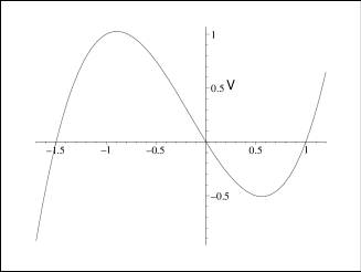
Figure 1: A typical scalar field potential, $V(\phi)$, for a transition from dS to AdS space.

Our strategy consists in using the Einstein equations in order to verify whether or not there exist consistent solutions with boundary conditions of the form (9). Using a technique introduced in ref. [9], we substract equations (14) and (15) which leads to

$$\left[a^{(d-2)}\left(h^{\prime}-h\frac{a^{2^{\prime}}}{a^{2}}\right)\right]^{\prime}=0.$$ (17)

This equation can be written like

$$\left(a^{d}\left(\frac{h}{a^{2}}\right)^{\prime}\right)^{\prime}=0,$$ (18)

which has a solution of the form

$$h(r)=a^{2}(r)\left(k_{1}\int_{0}^{r}\frac{dr^{\prime}}{a(r^{\prime})^{d}}+k_{2}\right),$$ (19)

where $k_{1}$ and $k_{2}$ are constants of integration. Imposing the dS/AdS boundary conditions (9) we obtain

$$k_{1}=2\left(\int_{-\infty}^{+\infty}\frac{dr^{\prime}}{a(r^{\prime})^{d}}\right)^{-1},$$ (20)

$$k_{2}=\frac{k_{1}}{2}\left(\int_{-\infty}^{0}\frac{dr^{\prime}}{a(r^{\prime})^{d}}-\int_{0}^{\infty}\frac{dr^{\prime}}{a(r^{\prime})^{d}}\right).$$ (21)

We note that the case when the absolute value of the cosmological constant is the same close to both boundaries ($l_{\scriptscriptstyle dS}=l_{\scriptscriptstyle AdS}$) corresponds to $a(r)=\pm a(-r)$. For example, this implies $k_{2}=0$ when the number of dimensions $d$ is even. Finally, by subtracting eqs. (13) and (14) we get

$$\frac{a^{\prime\prime}}{a}=-(d-1)(\phi^{\prime})^{2}.$$ (22)

In the appendix we describe in more details the properties of a real scalar field in a gravitational background of the form (1).

Let us now write down eq. (22) for general matter fields,

$$\frac{a^{\prime\prime}}{a}=\frac{T^{t}_{t}-T^{r}_{r}}{(d-2)h}.$$ (23)

In the region containing the boundary of AdS ($r>0$) we have $h(r)>0$. The variable $t$ is then the timelike coordinate and $T^{t}_{t}-T^{r}_{r}$ can be written like $-(\rho+p_{r})$ where $\rho$ and $p_{r}$ are respectively the energy density and the principal pressure along the coordinate $r$. In the region of space with a dS boundary we have $h(r)<0$ and $r$ is a timelike coordinate. This means that the combination $T^{t}_{t}-T^{r}_{r}$ is $(\rho+p_{t})$ where $p_{t}$ is the principal pressure along the spacelike coordinate $t$. The weakest of the gravitational energy conditions states (without proof) that a ‘reasonable’ gravitating system must be such that $T_{\mu\nu}n^{\mu}n^{\nu}\geq 0$ where $n^{\mu}$ is a null vector. In our case this means that any region of the spacetime should have $\rho+p\geq 0$ where $p$ stands for all principal pressures taken individually. The weak energy condition therefore requires that solutions associated with a ‘reasonable’ system have the property

$$\frac{a^{\prime\prime}}{a}=-\frac{\rho+p}{d-2}\leq 0,$$ (24)

which restricts considerably the number of possible candidate solutions for dS/AdS spacetimes.

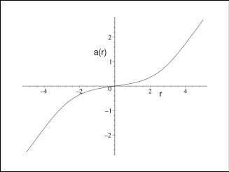
Figure 2: Example of a function $a(r)$ with the boundary conditions $a(r\rightarrow\pm\infty)=r/l_{(A)dS}$ where we have set $l_{(A)dS}=1$. This curve has $a^{\prime\prime}>0$ for $r>0$ and $a^{\prime\prime}<0$ for $r<0$.

4 No go theorem for dS/AdS spacetimes

In order to be acceptable, an asymptotically dS and AdS (dS/AdS) solution must have the following three properties: (1) its boundary conditions must be those specified in eq. (9), (2) the weak energy condition (equivalent to requiring $a^{\prime\prime}/a\leq 0$ everywhere) must be satisfied, and, (3) it must not develop curvature singularities. We address these issues in turn.

4.1 Boundary behavior and weak energy condition

There are four possible boundary conditions for dS/AdS solutions. The first two possibilities correspond to

$$\lim_{r\rightarrow+\infty}a(r)=+\frac{r}{l_{\scriptscriptstyle AdS}}\;\;\;\;\;{\rm and}\;\;\;\;\;\lim_{r\rightarrow-\infty}a(r)=+\frac{r}{l_{\scriptscriptstyle dS}},$$ (25)

or,

$$\lim_{r\rightarrow+\infty}a(r)=-\frac{r}{l_{\scriptscriptstyle AdS}}\;\;\;\;\;{\rm and}\;\;\;\;\;\lim_{r\rightarrow-\infty}a(r)=-\frac{r}{l_{\scriptscriptstyle dS}}.$$ (26)

If $l_{\scriptscriptstyle dS}=l_{\scriptscriptstyle AdS}$ these cases correspond to $a(r)=-a(-r)$. Figures 2 and 3 show functions with the boundary behavior (25). Functions such as the one represented in figure 2 are not solutions to the equation of motion (24) since they have $a^{\prime\prime}/a\geq 0$. Functions of the type shown on figure 3 are such that $a^{\prime\prime}<0$ for $r>0$ and $a^{\prime\prime}>0$ for $r<0$ which means they are acceptable candidate solutions. It is important to note that functions with the boundary conditions (25) and (26) always have at least one zero.

The remaining two boundary behaviors that can be considered are

$$\lim_{r\rightarrow+\infty}a(r)=+\frac{r}{l_{\scriptscriptstyle AdS}}\;\;\;\;\;{\rm and}\;\;\;\;\;\lim_{r\rightarrow-\infty}a(r)=-\frac{r}{l_{\scriptscriptstyle dS}},$$ (27)

or

$$\lim_{r\rightarrow+\infty}a(r)=-\frac{r}{l_{\scriptscriptstyle AdS}}\;\;\;\;\;{\rm and}\;\;\;\;\;\lim_{r\rightarrow-\infty}a(r)=+\frac{r}{l_{\scriptscriptstyle dS}}.$$ (28)

This corresponds to $a(r)=a(-r)$ if we set $l_{\scriptscriptstyle dS}=l_{\scriptscriptstyle AdS}$. Figure 4 shows a function with such boundary conditions. These functions always have at least one minimum which implies that $a^{\prime\prime}/a>0$ at least in a small region. This in turn means that eq. (24) is not satisfied. Consequently, because they violate the weak energy condition, solutions behaving like (27) and (28) are rejected.

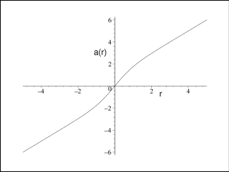
Figure 3: Example of a function $a(r)$ with boundary conditions $a(r\rightarrow-\infty)=r/l_{\scriptscriptstyle dS}$ and $a(r\rightarrow+\infty)=r/l_{\scriptscriptstyle AdS}$ where we have set $l_{\scriptscriptstyle dS}=1=l_{\scriptscriptstyle AdS}$. This example has $a^{\prime\prime}/a\leq 0$ everywhere.

4.2 Curvature singularities

We have found that there exists solutions $a(r)$ with the boundary conditions (9) that are not violating the energy conditions. The function $a(r)$ then has an asymptotic behavior given either by eq. (25) or eq. (26). These solutions typically have a zero for some finite value of $r$. We show that this leads to a curvature singularity. In fact, just by inspection of eq. (19) it seems that $h(r)$ will diverge when $a(r)=0$. The presence of curvature singularities can be investigated by studying the behavior of the curvature invariants $R$, $R_{\mu\nu}R^{\mu\nu}$ and $R_{\mu\nu\rho\sigma}R^{\mu\nu\rho\sigma}$. These typically involve the following terms,

$$h\frac{a^{\prime\prime}}{a},\;h^{\prime}\frac{a^{\prime}}{a},\;h^{\prime\prime},\;h\left(\frac{a^{\prime}}{a}\right)^{2}.$$ (29)

From (29) it appears that whenever $h(r)$ and/or its derivatives diverge a curvature curvature singularity will appear. To illustrate how $h(r)$ itself diverges where $a(r)=0$, we consider a subset of solutions for which $a(r)=-a(-r)$. We set $l_{\scriptscriptstyle dS}=1=l_{\scriptscriptstyle AdS}$ to simplify the analysis. These solutions must have the property,

$$\lim_{r\rightarrow 0^{\pm}}a(r)=a_{n}r^{n}\;\;\;\;\;{\rm no\;sum},$$ (30)

where $n$ is an integer and $a_{0}=0$. Using eq. (19) we obtain

$$\lim_{r\rightarrow 0^{\pm}}h(r)=\frac{k_{1}}{1-nd}r^{1-n(d-2)}+k_{2}r^{2n}.$$ (31)

Finiteness of this expression requires that

$$0\leq n\leq\frac{1}{d-2},$$ (32)

which is only satisfied for $n=1$ and $d=3$. We conclude that for $d>3$ the function $h(r)$ always diverges when $a(r)=0$. Next we consider how $a^{\prime}/a$ behaves when $a(r)=0$. Using (30) we find

$$\lim_{r\rightarrow 0^{\pm}}\frac{a^{\prime}}{a}=\frac{n}{r},$$ (33)

which clearly diverges. This divergence of $a^{\prime}/a$ is quite generic for all $d$ so the curvature invariants for $d=3$ will diverge as well.

We showed that solutions with the property $a(r)=-a(-r)$ generically develop a curvature singularity at $r=0$. This also applies to more general solutions for which $l_{\scriptscriptstyle dS}\neq l_{\scriptscriptstyle AdS}$. In other words this statement is true for all solutions with boundary conditions of the form (25) or (26). We note for future reference that solutions of the form shown in figure 4 with boundary conditions (27) are perfectly well-behaved. This statement can be traced to the fact that $a(r)$ does not have zeroes in this case. It is unfortunate that these functions are not solutions to the Einstein equations when the matter content of the theory respects the weak energy condition.

The results of this section allows us to formulate the following simple theorem:

No go theorem for dS/AdS transitions: Einstein gravity coupled to matter obeying the weak energy condition has no solutions corresponding to a dynamical system evolving from an asymptotic region containing a de Sitter (anti-de Sitter) boundary to another region that includes an anti-de Sitter (de Sitter) boundary.

Of course this possibly excludes spacetimes without boundaries and most certainly does not address spacetimes for which the evolution is quantum mechanically driven. For example, instanton solutions easily evade the no go theorem since they typically violate the energy conditions.

4.3 Regular solutions violating the energy conditions

The weak energy condition proposes that all physical systems have $\rho+p\geq 0$. We found that solutions $a(r)$ to eq. (23) with the boundary conditions (9) and for which the weak energy condition is satisfied do not exist. We also found that if the weak energy condition is relaxed, regular solutions are easily obtained. For example, the solution illustrated on figure 4 does not lead to any curvature singularity. Given such a solution, $h(r)$ can easily be obtained using eq. (19) which gives a full characterization of the dS/AdS spacetime.

We therefore conclude that there exist regular dS/AdS solutions only when energy conditions are violated. Interesting examples of such spacetimes are found in theories containing scalar fields with a kinetic term of the wrong sign ($\phi\rightarrow i\phi$ in (10)). In fact, the equation of motion (22) then becomes

$$\frac{a^{\prime\prime}}{a}=(d-1)(\phi^{\prime})^{2},$$ (34)

which, as shown above, does have regular solutions. The Type II* supergravity theories introduced in ref. [1, 2] generically contain fields with kinetic terms of the wrong sign. These theories are therefore natural laboratories where dS/AdS solutions might be investigated further.

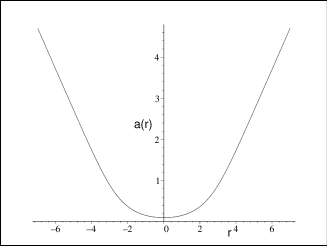
Figure 4: Example of a function $a(r)$ with boundary conditions $a(r\rightarrow-\infty)=-r/l_{\scriptscriptstyle dS}$ and $a(r\rightarrow+\infty)=r/l_{\scriptscriptstyle AdS}$ where we have set $l_{\scriptscriptstyle dS}=1=l_{\scriptscriptstyle AdS}$. This curve has $a^{\prime\prime}/a\geq 0$ for all values of $r$.

4.4 Asymptotically (A)dS geometries

We generalize our analysis to include asymptotically dS (dS/dS) and asymptotically AdS (AdS/AdS) spacetimes. The metric ansatz (1) can be used to describe asymptotically dS spacetimes when $h(r)=-a^{2}(r)$,

$$ds^{2}=-\frac{1}{a^{2}(r)}dr^{2}+a^{2}(r)\left(dt^{2}+d{\bf x}^{2}\right).$$ (35)

Using a change of coordinates of the form

$$dr^{2}/a^{2}(r)=d\rho^{2}$$ (36)

takes the metric to a more familiar expression, i.e.,

$$ds^{2}=-d\rho^{2}+a^{2}(\rho)\left(dt^{2}+d{\bf x}^{2}\right)$$ (37)

which corresponds to a foliation with flat constant $\rho$ spacelike slices. Similarly, metrics suitable for the study of AdS/AdS spacetimes are obtained by setting $h(r)=a^{2}(r)$ in (1) which leads to

$$ds^{2}=\frac{1}{a^{2}(r)}dr^{2}+a^{2}(r)\left(-dt^{2}+d{\bf x}^{2}\right).$$ (38)

Using the change of coordinates (36) this metric becomes

$$ds^{2}=d\rho^{2}+a^{2}(\rho)\left(-dt^{2}+d{\bf x}^{2}\right),$$ (39)

which corresponds to a foliation with flat Lorentzian slices. When considering metric ansatz (35) and (38), the boundary conditions corresponding to asymptotically (A)dS geometries are

$$\lim_{r\rightarrow\pm\infty}a^{2}(r)=\frac{r^{2}}{l^{2}_{(A)dS}}.$$ (40)

This last condition is equivalent to requiring that there are two (A)dS boundaries in the spacetime.

The boundary conditions (40) are the same as those used for dS/AdS spacetimes. The analysis we performed in section 4 can therefore easily be extended to (A)dS/(A)dS geometries. In fact, a certain combination of the Einstein equations again leads to the constraint

$$\frac{a^{\prime\prime}}{a}=-\frac{\rho+p}{(d-2)},$$ (41)

where the weak energy condition dictates that $\rho+p\geq 0$. We have shown in section 4 that there are no regular solutions $a(r)$ with boundary conditions (40) respecting the weak energy condition. The only exception in this case is $a(r)=r^{2}$ which corresponds to pure (A)dS space. We comment on that special case at the end of this section. Our result for (A)dS/(A)dS spacetimes does not imply that such geometries do not exist. The correct statement is that there are no (A)dS/(A)dS spacetimes for which two boundaries can be seen when the metric ansatz assumes a foliation by flat ($d-1$)-dimensional hypersurfaces.

A generating technique for AdS/AdS spacetimes was introduced in ref. [11] and generalized to dS/dS geometries in ref. [12]. We now show that solutions such as those typically only include one boundary which means that our metric ansatz (1) with boundary conditions (9) excludes them. For metrics of the form (37) and (39) one of the Friedmann equations can be written like,

$$\ddot{(\ln a)}=-\frac{\rho+p}{d-2},$$ (42)

where a ‘dot’ signifies a derivative with respect to the variable $\rho$. The only type of function which solves this equation is $\ln a$ of the form represented on figure 3. This corresponds to a scale factor with the boundary conditions,

$$\lim_{\rho\rightarrow+\infty}a(\rho)=e^{\rho/l^{f}_{(A)dS}},\;\;\;\;\;\lim_{\rho\rightarrow-\infty}a(\rho)=e^{\rho/l^{i}_{(A)dS}},$$ (43)

where the upper indices $i$ and $f$ respectively label the length scales as $r\rightarrow-\infty$ and $r\rightarrow+\infty$. Therefore we find that the scale factor vanishes for $r=-\infty$ which means that this region corresponds to an horizon, not a boundary. These solutions are regular (no curvature singularity) asymptotically (A)dS spacetimes. It is easy to demonstrate that these spacetimes cannot be written in the form (35) and (38). Using the appropriate change of coordinates we get,

$$r(\rho)=r(0)+\int_{0}^{\rho}a(\rho^{\prime})d\rho^{\prime},$$ (44)

but since $a(\rho\rightarrow-\infty)=0$ we see that the domain of $r$ is limited to positive values while the metric ansatz (35) and (38), in order to include two boundaries, had to be such that $-\infty<r<+\infty$.

A global metric for pure dS space:

We have indicated previously that the metric

$$-\frac{l^{2}}{r^{2}}dr^{2}+\frac{r^{2}}{l^{2}}\left(dt^{2}+d{\bf x}^{2}\right),$$ (45)

corresponds to a solution to the Einstein equations with a cosmological constant,

$$\Lambda=\frac{(d-1)(d-2)}{2l^{2}}.$$ (46)

This solution corresponds to a foliation of dS space with flat constant $r$ hypersurfaces. Eq. (45) for dS is global in the sense that it covers the whole spacetime. This can be seen by using the change of coordinates $r=\pm l\,e^{\pm\tau/l}$. The original metric then becomes

$$ds^{2}=-\frac{1}{l^{2}}d\tau^{2}+e^{\pm 2\tau/l}\left(dt^{2}+d{\bf x}^{2}\right),$$ (47)

where $-\infty<\tau<+\infty$. Expressions (47) represent the two inflationary patches of dS space. The Big Bang patch (containing the boundary $I^{+}$ and corresponding to the plus sign in (47)) is covered by the system of coordinates (45) for $-\infty<r<0$. The Big Crunch patch of dS (containing the boundary $I^{-}$ and corresponding to the minus sign in (47)) is covered by (45) when $0<r<+\infty$. Therefore the coordinate system (45) for pure dS covers the whole spacetime with flat ($d-1$)-dimensional hypersurfaces.

5 Discussion

We used Einstein gravity coupled to general matter fields in order to prove that when the weak energy condition is respected there cannot be non-singular solutions which extrapolate between an asymptotically de Sitter region containing a boundary and an asymptotically anti-de Sitter region containing a boundary. This result is quite generic. For example, there is no dS/AdS solutions in any of the conventional supergravity theories. Exceptions might appear when one considers sources in the form of such stringy objects as orientifold planes and negative tension branes which typically violate the weak energy condition (see, for example, [13]).

We conclude this presentation by discussing ideas from both the AdS/CFT and the dS/CFT in order to initiate a discussion as to how dS/AdS spacetimes might be interpreted in the context of gauge/gravity dualities. In the AdS/CFT correspondence, quantum gravity in pure AdS space is conjectured to be dual to a conformal field theory in one less dimension that can be regarded as being defined on the boundary of the bulk spacetime. For AdS in Poincaré coordinates,

$$ds^{2}=dr^{2}+e^{2r/l_{\scriptscriptstyle AdS}}\left(-dt^{2}+d{\bf x}^{2}\right),$$ (48)

the boundary is located at $r=+\infty$. The dS/CFT correspondence analogously proposes that quantum gravity in dS space has a Euclidean conformal field theory dual defined on its boundary(ies). When formulated using inflationary coordinates,

$$ds^{2}=-dr^{2}+e^{-2r/l_{\scriptscriptstyle dS}}\left(dr^{2}+d{\bf x}^{2}\right),$$ (49)

the spacelike boundary of dS space, $I^{-}$, is located at $r=-\infty$. In this paper we investigated solutions interpolating between asymptotic regions of the form eq. (48) and (49) and their $r\rightarrow-r$ counterparts.

A more general formulation of the AdS/CFT and the dS/CFT dualities considers an equivalence between asymptotically (A)dS spacetimes and non-conformal field theories. In the context of the AdS/CFT correspondence, this leads to the so-called UV/IR correspondence[14, 15] stating that asymptotic regions (near the boundary) of AdS space are associated with short distance (UV) physics in the field theory dual while regions deeper in the AdS are related to long distance (IR) physics. It is then natural to associate evolution along the $r$-coordinate with a field theory renormalization group (RG) flow. An interesting result then is the derivation of a gravitational c-theorem[16]. The corresponding c-function is a local geometric quantity which gives a measure of the number of degrees of freedom relevant for physics in the dual field theory at different energy scales. Requiring gravitational energy conditions to be satisfied indicates that this c-function must decrease in evolving from the UV toward the IR regions, as expected. Ideas along the same lines can be used in the context of the dS/CFT correspondence. Again demanding energy conditions to hold leads to a gravitational c-theorem for asymptotically dS spacetimes[4, 5, 12]. The latter states that the c-function must decrease (increase) in a period of contraction (expansion). For example, when considering spacetimes with both asymptotia (at $r=\pm\infty$) of the form (49), the boundary $I^{-}$ corresponds to the UV while the horizon at $r=+\infty$ is interpreted as an IR limit of the field theory.

Let us begin by considering spacetimes with two boundaries located at $r=\pm\infty$. These spacetimes could be (A)dS/(A)dS or the mixed geometries dS/AdS introduced in this paper. Following ref. [12] we define an effective cosmological constant

$$\Lambda_{\scriptstyle eff}=-G_{\mu\nu}n^{\mu}n^{\nu},$$ (50)

where $n^{\mu}$ is unit vector normal to the constant $r$ hypersurfaces. Expression (50) in fact reduces to eqs. (7) and (3) when evaluated respectively for the spacetimes (48) and (49). A reasonable definition for the c-function is

$$c\sim\frac{1}{G_{\scriptscriptstyle N}|\Lambda_{\scriptstyle eff}^{(d-2)/2}|}=\frac{1}{G_{\scriptscriptstyle N}}|-G_{\mu\nu}n^{\mu}n^{\nu}|^{-(d-2)/2}.$$ (51)

Of course, introducing a gravitational c-function is relevant only if the gravitational background under consideration has a field theory dual. In the case of spacetimes interpolating between regions with dS and AdS boundaries, it would be interesting to find out what kind of field theory, if any, could be the dual. While we cannot address this question to a satisfactory level at this point, one thing we can do is describe roughly the rather strange field theory RG flow such a peculiar gravitational background would be dual to. The existence of such a mixed (dS/AdS)/CFT correspondence would imply that the bulk coordinate which is reconstructed by the field theory RG flow is timelike in the region containing the dS boundary and spacelike in the region containing the AdS boundary. Let us for the moment assume that the weak energy condition, which was used in deriving the c-theorems associated to AdS/CFT and dS/CFT correspondences, holds everywhere in the corresponding gravitational dual. We would then expect the following to hold: The boundary at $r=+\infty$ (AdS) corresponds to physics in the conformal UV limit of the field theory. The weak energy condition being satisfied for $r>0$, we expect that translations along decreasing $r$, i.e., moving deeper inside of the spacetime, corresponds to flowing toward an IR region close to $r=0$. Past the horizon, the variable $r$ becomes timelike which means that the RG flow should now describe a limit of the field theory which is Euclidean. Since the weak energy condition is still assumed to hold for $r<0$, the c-theorem guarentees that evolving toward increasingly negative values of $r$ corresponds to ‘integrating in’ degrees of freedom, i.e., moving toward another UV fixed point, this time defined on the spacelike boundary $I^{-}$. Since both these UV fixed points appear to be flowing toward the same IR limit, it would be tempting to postulate a new self-duality for the field theory. The latter would be a rather strange duality between a Lorentzian and a Euclidean limit of the same field theory. In this paper we found evidence that such spacetimes do not exist. We have found that dS/AdS gravitational backgrounds can exist only when energy conditions are violated in which case the c-theorems are not valid anymore. Because they contain fields with kinetic terms of the wrong sign, the type II* theories may be a good place where dS/AdS geometries and consequently their field theory dual can be studied.

Appendix A Energy conditions and equation of state for scalars

In this appendix we comment on the energy conditions and the equation of state associated with a real scalar field in a gravitational background of the form (1). The stress-energy tensor components for a real scalar field are

$$T^{r}_{r}=-\frac{(d-1)(d-2)}{2}\left[-h\phi^{{}^{\prime}2}+V(\phi)\right],$$ (52)

$$T^{t}_{t}=T_{x}^{x}=-\frac{(d-1)(d-2)}{2}\left[h\phi^{{}^{\prime}2}+V(\phi)\right].$$ (53)

For $r>0$, i.e., in the region containing the AdS boundary, the components of the stress-energy tensor are

$$\rho=-T_{t}^{t}=\frac{(d-1)(d-2)}{2}\left[h\phi^{{}^{\prime}2}+V(\phi)\right],$$ (54)

$$p_{x}=T_{x}^{x}=-\frac{(d-1)(d-2)}{2}\left[h\phi^{{}^{\prime}2}+V(\phi)\right],$$ (55)

and

$$p_{r}=T_{r}^{r}=-\frac{(d-1)(d-2)}{2}\left[-h\phi^{{}^{\prime}2}+V(\phi)\right],$$ (56)

where $\rho$ is the conserved energy density associated with the Killing direction $t$ and $p_{r}$, $p_{x}$ are the principal pressures respectively along the directions $r$ and $x^{a}$. For $r>0$ we have an anisotropic fluid since $p_{r}\neq p_{x}$. There are two equations of state:

$$\frac{p_{x}}{\rho}=-1,$$ (57)

and

$$\frac{p_{r}}{\rho}=\frac{h\phi^{{}^{\prime}2}-V(\phi)}{h\phi^{{}^{\prime}2}+V(\phi)}.$$ (58)

Pure AdS and dS space have $p/\rho=-1$ where $p$ represents all principal pressures. In our case, the quantity $h\phi^{2^{\prime}}+V(\phi)$ is conserved but not $h\phi^{2^{\prime}}-V(\phi)$ which means that their ratio $p_{r}/\rho$ depends on the variable $r$. In order to have an asymptotic $r\rightarrow+\infty$ region corresponding to AdS we must therefore have

$$\lim_{r\rightarrow+\infty}\frac{h\phi^{{}^{\prime}2}}{V(\phi)}=0.$$ (59)

In the region containing the dS boundary ($r<0$) we have

$$\rho=-T_{r}^{r}=\frac{(d-1)(d-2)}{2}\left[-h\phi^{{}^{\prime}2}+V(\phi)\right],$$ (60)

$$p=p_{t}=p_{x}=T^{t}_{t}=-\frac{(d-1)(d-2)}{2}\left[h\phi^{{}^{\prime}2}+V(\phi)\right],$$ (61)

which corresponds to the equation of state

$$\frac{p}{\rho}=\frac{h\phi^{{}^{\prime}2}+V(\phi)}{h\phi^{{}^{\prime}2}-V(\phi)},$$ (62)

which again goes to $p/\rho=-1$ for large negative $r$ when eq. (59) is satisfied. We note that for $r<0$ the energy density $\rho$ is not conserved since there is no Killing vector associated with the direction $r$. This is of course expected for a time dependent background.

For $r<0$ we have

$$\rho+p_{x}=0,$$ (63)

and $\rho+p_{r}=(d-1)(d-2)h(r)\phi^{{}^{\prime}2}.$ Since $h(r)>0$ for $r>0$ we have $\rho+p\geq 0$ in that region. Now for $r<0$ we find

$$\rho+p=-(d-1)(d-2)h\phi^{{}^{\prime}2},$$ (64)

which is such that $\rho+p\geq 0$ since $h(r)<0$ for $r<0$. It is therefore easy to see that scalar fields do not violate any of the energy conditions.

References

- [1] C. M. Hull, “Timelike T-duality, de Sitter space, large N gauge theories and topological field theory,” JHEP 9807, 021 (1998), hep-th/9806146.
- [2] C. M. Hull, “de Sitter space in supergravity and M theory,” JHEP 0111, 012 (2001), hep-th/0109213.
- [3] A. Strominger, “The dS/CFT correspondence,” JHEP 0110, 034 (2001), hep-th/0106113].
- [4] A. Strominger, “Inflation and the dS/CFT correspondence,” JHEP 0111, 049 (2001), hep-th/0110087.
- [5] V. Balasubramanian, J. de Boer, and D. Minic, “Mass, Entropy, and Holography in Asymptotically de Sitter spaces” hep-th/0110108].
- [6] E. Witten, “Quantum gravity in de Sitter space, hep-th/0106109.
- [7] O. Aharony, S.S. Gubser, J. Maldacena, H. Ooguri and Y. Oz, “Large N field theories, string theory and gravity,” Phys. Rept. 323,183 (2000), hep-th/9905111.
- [8] M. Spradlin, A. Strominger and A. Volovich, “Les Houches lectures on de Sitter space,” arXiv:hep-th/0110007.
- [9] J. M. Cline and H. Firouzjahi, “No-go theorem for horizon-shielded self-tuning singularities,” Phys. Rev. D 65, 043501 (2002) [arXiv:hep-th/0107198].
- [10] M. K. Parikh, I. Savonije and E. Verlinde, “Elliptic de Sitter space: dS/Z(2),” arXiv:hep-th/0209120.
- [11] O. DeWolfe, D. Z. Freedman, S. S. Gubser and A. Karch, “Modeling the fifth dimension with scalars and gravity,” Phys. Rev. D 62, 046008 (2000) [arXiv:hep-th/9909134].
- [12] F. Leblond, D. Marolf and R. C. Myers, “Tall tales from de Sitter space. I: Renormalization group flows,” JHEP 0206, 052 (2002), hep-th/0202094.
- [13] D. Marolf and S. F. Ross, “Stringy negative-tension branes and the second law of thermodynamics,” JHEP 0204, 008 (2002) [arXiv:hep-th/0202091].
- [14] L. Susskind and E. Witten, “The holographic bound in anti-de Sitter space,” hep-th/9805114.
- [15] A.W. Peet and J. Polchinski, “UV/IR relations in AdS dynamics,” Phys. Rev. D 59, 065011 (1999), hep-th/9809022.
-
[16]
D.Z. Freedman, S.S. Gubser, K. Pilch and N.P. Warner,
“Renormalization group flows from holography supersymmetry and a
Adv. Theor. Math. Phys. 3, 363 (1999), hep-th/9904017;
J. de Boer, E. Verlinde and H. Verlinde, “On the holographic renormalization group,” JHEP 0008, 003 (2000), hep-th/9912012;
V. Balasubramanian, E.G. Gimon and D. Minic, “Consistency conditions for holographic duality,” JHEP 0005, 014 (2000), hep-th/0003147;
V. Sahakian, “Holography, a covariant c-function and the geometry of the renormalization group,” Phys. Rev. D 62, 126011 (2000), hep-th/9910099;
E. Alvarez and C. Gomez, “Geometric holography, the renormalization group and the c-theorem,” Nucl. Phys. B 541, 441 (1999), hep-th/9807226.