Tadpole Analysis of Orientifolded Plane-Waves

Abstract:

We study orientifolds of type IIB string theory in the plane-wave background supported by null RR 3-form flux $F^{(3)}$. We describe how to extract the RR tadpoles in the Green-Schwarz formalism in a general setting. Two models with orientifold groups $\{1,\Omega\}$ and $\{1,\Omega\,I_{4}\}$, which are T-dual to each other, are considered. Consistency of these backgrounds requires 32 D9 branes for the first model and 32 D5 branes for the second one. We study the spectra and comment on the heterotic duals of our models.

1 Introduction

It has recently emerged that type IIB string theory admits supersymmetric plane-wave backgrounds [1, 2] supported by Ramond-Ramond (RR) fluxes. String theory in these backgrounds turns out to be solvable in the light-cone Green-Schwarz(GS) formalism for both closed [3, 4, 6] and open strings [7, 8, 9, 10, 11]. Many of these backgrounds can be obtained as Penrose limits of known ones. This fact enables understanding of their holographic duals in terms of some sectors of the CFT dual to the original background [5].

It is well known that one can generate new vacua of string theory by gauging a subgroup of discrete symmetries. For instance, the symmetry group of type IIB string theory in the Minkowski space contains the following discrete subgroup:

$${\cal G}=\{1,\Omega,(-1)^{F_{L}},(-1)^{F_{R}},(-1)^{F_{s}},\Omega(-1)^{F_{L}},\Omega(-1)^{F_{R}},\Omega(-1)^{F_{s}}\}$$ (1)

where $\Omega$ represents the world-sheet parity operator, $(-1)^{F_{L}}$ and $(-1)^{F_{R}}$ represent the space-time fermion number operators coming from the world-sheet left movers and the right movers respectively and $(-1)^{F_{s}}\equiv(-1)^{F_{L}+F_{R}}$. One can consider various subgroups of ${\cal G}$ and gauge them to obtain new vacua. Orientifolds are the vacua obtained by gauging a discrete subgroup which contains at least one element with $\Omega$. A simple example is the type I theory with $SO(32)$ gauge group obtained as an orientifold of type IIB by the group $\{1,\Omega\}$.

With the new plane-wave vacua of string theory at hand it is natural and interesting to study their orientifolds. In [8] the authors have considered the orientifold of type IIB theory in the background of the maximally supersymmetric plane-wave supported by a null RR 5-form flux [1]. More orientifold models have been considered in [12]. In this paper we would like to explore orientifolds of type IIB in the background of the supersymmetric plane-wave

$$ds^{2} = dx^{+}dx^{-}-f^{2}x^{i}x^{i}(dx^{+})^{2}+dx^{i}dx^{i}+dx^{\alpha}dx^{\alpha}$$ (3)

$$~{}~{}~{}F^{(3)}_{+12}=F^{(3)}_{+34}=-2f.$$

where $F^{(3)}$ is the field strength of the RR two form of type IIB, $i=1,2,3,4$ are the indices along the plane-wave but transverse to the light cone directions $(x^{+},x^{-})$ and $\alpha=5,6,7,8$ are four flat directions transverse to the plane-wave.

The background (3) can be obtained as a Penrose limit of $AdS_{3}\times S^{3}\times T^{4}$ solution of type IIB. The world-sheet theory of closed strings in this background has been solved in the Green-Schwarz light-cone formulation in [5, 6]. Similarly, open strings in this background have been quantized in [10].

For constructing an orientifold of this background, we first note that the world-sheet parity operator $\Omega$ generates a symmetry of this model because the RR 2–form is invariant under the action of $\Omega$. Therefore, one could gauge this symmetry combined with some discrete space-time symmetry and extract the resultant theory. For example type IIB on (3) admits the following discrete symmetry groups: (i) $\{1,\Omega\}$, (ii) $\{1,\Omega I_{4}\}$ where $I_{4}$ is reflection along four of the eight coordinates transverse to the light-cone direction with the condition that the reflection $I_{4}$ leaves the RR field invariant, (iii) $\{1,\Omega I_{8}\}$ where $I_{8}$ is reflection of all $x^{i}$ and $x^{\alpha}$.

In this paper we consider the following two models:

1. Type IIB on PP${}_{6}\times{\mathbb{R}}^{4}$/$\{1,\Omega\}$

2. Type IIB on PP${}_{6}\times T^{4}$/$\{1,\Omega I_{5678}\}$

where we have denoted the space-time of (3) along $(x^{+},x^{-},x^{1},x^{2},x^{3},x^{4})$ directions by PP₆. Typically, orientifolds suffer from tadpole divergences. For the consistency of the theory, one has to ensure that such tadpoles are absent. For example, type IIB on ${\mathbb{R}}^{9,1}$/$\{1,\Omega\}$ has a non-vanishing RR 10–form tadpole. This is cancelled by introducing 32 D9–branes in the vacuum. In what follows, we analyze the RR tadpoles for the models above.

In section 2, we review the RR tadpole calculation from the point of view of the NSR formalism . We then describe how to extract the RR exchange contributions of the Cylinder(C), Möbius strip(MS) and Klein Bottle(KB) diagrams using the light-cone Green-Schwarz formulation. In section 3, we describe the action of the discrete symmetries on the states of the Hilbert space and use the results of section 2 to calculate the RR tadpoles of our models. We find that the RR tadpole cancellation requires 32 D9-branes in the first model and 32 D5 branes in the second model. One can arrange the spectrum of ‘massless’ states in representations of the isometry group. We carry out this analysis for the open string massless fields in detail for the first model. The plausible Heterotic dual description of our orientifold vacua are also considered. We conclude in section 4. Appendix A contains a review of the relevant features of closed and open strings quantization in the plane-wave background. Appendix B contains some details on the regularizations of the zero point energies of bosons and fermions in plane-wave backgrounds.

2 Revisiting the Orientifold

String theory in the background of plane-waves of the kind (3) with RR fields can be solved in the Green-Schwarz formalism in the light-cone gauge. As such, it is necessary to establish the rules for tadpole computations in the Green-Schwarz formalism. Before this, it is useful to briefly review how the RR tadpole is calculated in the NSR formalism[13, 14, 15, 16].

2.1 RR Tadpole in NSR Formalism

Recall that there are three diagrams at the one loop order in perturbative string theory with unoriented closed and open strings: the Klein bottle (KB), the Möbius strip (MS) and the Cylinder (C). The KB amplitude corresponds to the exchange of closed strings between two orientifold planes. The MS amplitude corresponds to that between an orientifold plane and a D-brane and C amplitude corresponds to that between two D-branes. Conformal invariance allows us to view these as either tree channel or loop channel diagrams. These two channels are related to each other by modular transformations of the corresponding diagrams. Let $l$ denote the modular parameter of a diagram in the tree channel ( a closed string of length $2\pi$ propagating for a time $2\pi l$) and $t$ denote that in the loop channel (a closed string of length $2\pi$ or an open string of length $\pi$ propagating for a time $2\pi t$). Then they are related to each other by the following equations.

$${\rm KB}:~{}~{}t={1\over 4l},~{}~{}~{}~{}\hbox{MS}:~{}~{}t={1\over 8l},~{}~{}~{}~{}{\rm C}:~{}~{}t={1\over 2l}.$$ (4)

The amplitudes can be expressed in terms of the following standard modular functions:

$$f_{1}(q) = q^{\frac{1}{12}}\prod_{n=1}^{\infty}(1-q^{2n}),~{}~{}~{}~{}~{}~{}~{}~{}\,f_{2}(q)=\sqrt{2}q^{\frac{1}{12}}\prod_{n=1}^{\infty}(1+q^{2n})$$ (5)

$$f_{3}(q) = q^{-\frac{1}{24}}\prod_{n=1}^{\infty}(1+q^{2n-1}),~{}~{}~{}~{}f_{4}(q)=q^{-\frac{1}{24}}\prod_{n=1}^{\infty}(1-q^{2n-1}).$$ (6)

These functions satisfy the Jacobi Identity (abstruse identity)

$$f_{3}^{8}(q)=f_{2}^{8}(q)+f_{4}^{8}(q)$$ (7)

and have the following modular transformation properties

$$f_{1}(e^{-\pi/s})=\sqrt{s}f_{1}(e^{-\pi s}),~{}~{}f_{3}(e^{-\pi/s})=f_{3}(e^{-\pi s}),~{}~{}f_{2}(e^{-\pi/s})=f_{4}(e^{-\pi s}).$$ (8)

One way to extract the tadpoles is to calculate the diagrams KB, MS and C in loop channel as traces over the open (for C and MS) or closed (for KB) string Hilbert space and convert them into tree channel using relations (4). The tadpoles arise in the limit $t\rightarrow 0$ (equivalently $l\rightarrow\infty$). In a supersymmetric theory with Bose-Fermi degeneracy at each level, all three amplitudes KB, MS and C vanish individually. In the loop channel, the vanishing is because of the Bose-Fermi degeneracy of the string spectrum. From the tree channel point of view, in the NSR formalism, they vanish because of the cancellation between the contributions of NSNS and the RR exchange amplitudes(though each of NSNS and RR fields give divergent contributions to the amplitude). For the RR tadpole cancellation, one has to extract the RR field contribution alone for all the diagrams, add them and require that the sum vanishes. For this one needs to analyze how the boundary conditions in tree channel map onto those in the loop channel.

For example, for the orientifold model Type IIB on ${\mathbb{R}}^{9,1}/\{1,\Omega\}$ one gets the following contributions to the RR exchange amplitude: $\frac{v_{10}}{256}\int_{0}^{\infty}{dt\over t^{6}}$ times

$${\rm KB} :~{}~{} 32\frac{f_{4}^{8}(e^{-2\pi t})}{f_{1}^{8}(e^{-2\pi t})}$$ (9)

$${\rm MS} :~{}~{} -\frac{f_{2}^{8}(e^{-2\pi t})f_{4}^{8}(e^{-2\pi t})}{f_{1}^{8}(e^{-2\pi t})f_{3}^{8}(e^{-2\pi t})}\{{\rm Tr}(\gamma_{\Omega}^{-1}\gamma_{\Omega}^{T})\}$$ (10)

$${\rm C} :~{}~{} \frac{f_{4}^{8}(e^{-\pi t})}{f_{1}^{8}(e^{-\pi t})}\{({\rm Tr}(\gamma_{1}))^{2}\}$$ (11)

where $v_{10}=V_{10}/(4\pi^{2}\alpha^{\prime})^{3}$ with $V_{10}$ being the regularized space-time volume, $\gamma_{\Omega}$ and $\gamma_{1}$ are the matrix representation of the elements $\Omega$ and $1$ respectively on the open-string Chan-Paton(CP) factors. To extract the tadpole consistency condition one factorizes this amplitude in the tree channel using the modular transformations (4, 8) to get

$$\frac{v_{10}}{16}\int_{0}^{\infty}dl\{32^{2}-64{\rm Tr}(\gamma_{\Omega}^{-1}\gamma_{\Omega}^{T})+({\rm Tr}(\gamma_{1}))^{2}\}.$$ (12)

For SO projection on the CP factors we have $\gamma_{\Omega}^{T}=\gamma_{\Omega}$ and one chooses $\gamma_{1}=1$. Since $\gamma_{\Omega}$ is symmetric for the SO projection, by a unitary change of basis one can make $\gamma_{\Omega}=1$. With this, expression in (12) becomes:

$$\frac{v_{10}}{16}\int_{0}^{\infty}dl\,(n_{9}-32)^{2}$$ (13)

where $n_{9}={\rm Tr}(1)$ is the number of D9-branes. Therefore the RR tadpole in this model vanishes for $n_{9}=32$ giving rise to the Type I theory with a gauge group SO(32).

2.2 RR Tadpole from Light-cone Green-Schwarz String

Unlike in the NSR case, in GS formalism there is no such straightforward way of interpreting the amplitudes in the tree channel. The aim of this subsection is to describe a method to extract the RR exchange contributions in the tree channel from the loop channel amplitudes in the GS formalism.

The basic idea is to use the fact that in the tree channel, we have contributions from the ‘NSNS’ and ‘RR’ fields exchanged and one can extract the RR contribution alone by inserting a projection operator which projects out the NSNS states. The operator that achieves this is $\frac{1-(-1)^{F_{L}}}{2}$ as the NSNS sector states are invariant and RR states change sign under $(-1)^{F_{L}}$. In what follows we carefully analyze the effect of the insertion of $\frac{1-(-1)^{F_{L}}}{2}$ in the tree channel on the loop channel amplitudes. We analyze the simple case of the orientifold group $\{1,\Omega\}$ below. This can be generalized to the other orientifold groups trivially. Let us consider the Cylinder diagram first.

2.2.1 The Cylinder

Firstly recall that in the NSR formalism, the tree channel cylinder amplitude can be thought of as the overlap of a boundary state $|Dp\rangle$ representing a Dp-brane propagated for a distance $l$ with itself and integrated over $l$,

$$C~{}~{}~{}~{}:~{}~{}~{}~{}\int_{0}^{\infty}dl\,\langle Dp|e^{-2\pi l\,H_{c}}|Dp\rangle.$$ (14)

This expression evaluates into the sum of contributions coming from the exchange of NSNS sector fields and from the RR sector fields. If we insert the operator ${1-(-1)^{F_{L}}\over 2}$ in (14), we recover the contribution coming only from the exchange of the RR sector fields alone. The fact that this is true in both NSR and GS formalism is going to be exploited.

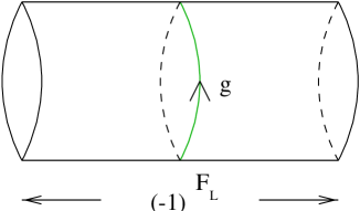
Figure 1: Cylinder diagram with $(-1)^{F_{L}}$ insertion in the tree channel.

To find the RR contribution of the cylinder diagram we start with the tree channel formula:

$$C~{}~{}~{}~{}:~{}~{}~{}~{}\int_{0}^{\infty}dl\,\langle Dp|({1\over 2}-{(-1)^{F_{L}}\over 2})\,e^{-2\pi\,l\,H_{c}}|Dp\rangle$$ (15)

and translate it into a loop channel amplitude. We take the ranges of the coordinates to be $0\leq\sigma^{1}\leq 2\pi l$, $0\leq\sigma^{2}\leq 2\pi$. The insertion of $1/2$ in (15) gives half of the amplitude in equation (14). On the other hand, the effect of the insertion of $(-1)^{F_{L}}/2$ on the boundary conditions for the fermions in the loop channel is as follows (see fig. (1)). The defining equation of the boundary state of the Dp-brane is, schematically, given by:

$$\left(S^{a}(\sigma^{2})+iM_{ab}\tilde{S}^{b}(\sigma^{2})\right)|Dp\rangle=0.$$ (16)

This translated into the loop channel means that the open string boundary condition is $S^{a}|_{\sigma^{1}}=M_{ab}\tilde{S}^{b}|_{\sigma^{1}}$ where $M_{ab}$ is an operator made of product of $SO(8)$ gamma matrices depending on the D-brane we want to describe and $\sigma^{1}$ is either $0$ or $\pi$. Insertion of $(-1)^{F_{L}}/2$ in the tree channel amounts to replacing the boundary state $|Dp\rangle$ at $\sigma^{1}=\pi$ by $(-1)^{F_{L}}/2|Dp\rangle$. Then Eq.(16) gives

$$\left(S^{a}(\sigma^{2})+iM_{ab}\tilde{S}^{b}(\sigma^{2})\right)|Dp\rangle=0$$ (17)

$$\Rightarrow (-1)^{F_{L}}\left(S^{a}(\sigma^{2})+iM_{ab}\tilde{S}^{b}(\sigma^{2})\right)(-1)^{2F_{L}}|Dp\rangle=0$$ (18)

$$\Rightarrow \left(S^{a}(\sigma^{2})-iM_{ab}\tilde{S}^{b}(\sigma^{2})\right)(-1)^{F_{L}}|Dp\rangle=0$$ (19)

where in the second line we have inserted $1=(-1)^{2F_{L}}$ and operated by $(-1)^{F_{L}}$ from the left. Converting this into the open string boundary conditions implies: $S^{a}|_{\sigma^{1}=\pi}=-M_{ab}\tilde{S}^{b}|_{\sigma^{1}=\pi}$. This makes the open string fermions half integer moded. That means the insertion of $(-1)^{F_{L}}$ in the tree channel picks the ‘wrong’ boundary conditions in the loop channel.

Therefore, we conclude that the RR contribution of the cylinder diagram in the loop channel in GS formalism is

$$\hbox{C}~{}~{}~{}:~{}~{}~{}\hbox{\bf Tr}_{{\cal H}_{o}}\left[\frac{1}{2}(-1)^{F_{s}}e^{-2\pi t\,\hbox{H}_{o}}\right]-\hbox{\bf Tr}_{\tilde{\cal H}_{o}}\left[\frac{1}{2}(-1)^{F_{s}}e^{-2\pi t\,\hbox{H}_{o}}\right],$$ (20)

where we have denoted the open string Hilbert space of $8\times\hbox{PB}\oplus 8\times\hbox{AF}$ by $\tilde{\cal H}_{o}$ where PB stands for a periodic boson and AF is an antiperiodic fermion. The operator $H_{o}$, which plays the role of $L_{0}$ (the Virasoro generator) in NSR formalism, is given by:

$$H_{o}=p^{+}(p^{-}+H^{o}_{l.c})$$ (21)

where $H^{o}_{l.c}$ is the light-cone Hamiltonian of the GS open string. The trace $\hbox{\bf Tr}_{\tilde{\cal H}_{o}}$ in (20) includes an integration over the bosonic zero modes (the center of mass coordinates and momenta) of the string and an integration $\int_{0}^{\infty}dt/2t$ over the modular variable of the cylinder. The operators inserted are simply determined by the requirement of the usual periodic light-cone GS fermions.

Heuristically, the half-integer moding was to be expected. The insertion of $(-1)^{F_{L}}$ converts $|Dp\rangle$ to $|{\bar{Dp}}\rangle$ and the $D-\bar{D}$ overlap now will have a tachyon in its spectrum which is consistent with half-integral moding.

2.2.2 Klein Bottle and Möbius Strip

Let us now obtain the corresponding formulae for the RR contributions to KB and MS diagrams. For this, it is useful to briefly review how to translate the quantities from tree channel to loop channel in these cases [13, 14].

Recall that to make a Klein bottle one can start with a torus with coordinates $0\leq\sigma^{1}\leq 4\pi l$ and $0\leq\sigma^{2}\leq 2\pi$ (with $\sigma^{1}\sim\sigma^{1}+4\pi l$ and $\sigma^{2}\sim\sigma^{2}+2\pi$) and make a $Z_{2}$ identification:

$$(\sigma^{1},\sigma^{2})\sim(4\pi l-\sigma^{1},\sigma^{2}+\pi).$$ (22)

One can choose two different fundamental regions and these two choices naturally correspond to tree channel and loop channel string diagrams (see figure 2). The prescription to go from the tree to loop channel is to (i) cut the upper half of tree channel diagram ($0\leq\sigma^{1}\leq 2\pi l$ and $\pi\leq\sigma^{2}\leq 2\pi$), (ii) invert it from right to left, (iii) multiply the fields by $\Omega^{-1}$ ( by $(\Omega h_{2})^{-1}$ in the general case where the orientifolding contains a space-time symmetry generator as well. See Fig.(3a)). and (iv) glue it to the right side of the lower half.

Figure 2: Two ways to view Klein Bottle

We are interested in going from the tree channel to loop channel when there is a $(-1)^{F_{L}}$ operator inserted in the tree as one goes from $0$ to $2\pi l$. Since in this case, there is an operator $(-1)^{F_{L}}$ in the upper half as well when we perform the step (iii) above it will turn into $(-1)^{F_{R}}$ since the action of multiplying by ${\cal O}\equiv\Omega^{-1}$ ($(\Omega{h_{2}})^{-1}$ in the general case) on the fields becomes conjugation by ${\cal O}$ on the operators. Therefore $(-1)^{F_{L}}\rightarrow{\cal O}^{-1}(-1)^{F_{L}}{\cal O}=(-1)^{F_{R}}$. Hence by the end of step (iv) we have the fields in the loop channel twisted by the operator $(-1)^{F_{L}}\times(-1)^{F_{R}}=(-1)^{F_{s}}$. Since the loop channel of KB is also a closed-string tree channel, both the left moving and right moving GS closed string fermions $\tilde{S}^{a}$ and $S^{a}$ are twisted by $(-1)^{F_{s}}$ giving rise to half-integer moding. Therefore, the full RR contribution to the Klein Bottle diagram is

$${\rm K.B}:~{}~{}~{}~{}\hbox{\bf Tr}_{{\cal H}_{c}}\left[\frac{\Omega}{2}(-1)^{F_{s}}\,e^{-2\pi t\,\hbox{H}_{c}}\right]-\hbox{\bf Tr}_{\tilde{{\cal H}}_{c}}\left[\frac{\Omega}{2}(-1)^{F_{s}}\,e^{-2\pi t\,\hbox{H}_{c}}\right]$$ (23)

where the first term comes from the insertion of $1/2$ and the second one is from $(-1)^{F_{L}}/2$. where $\tilde{{\cal H}}_{c}$ denotes the fock space of $(8\times\hbox{PB}\oplus 8\times\hbox{AF})\otimes(8\times\hbox{PB}\oplus 8\times\hbox{AF})$. As in (21) $H_{c}=\frac{p^{+}}{2}(p^{-}+2H^{c}_{l.c})$ with $H^{c}_{l.c}$ the closed string light-cone Hamiltonian.

Figure 3: (a) Klein Bottle and (b) Möbius Strip

Now we turn to the Möbius Strip diagram. In this case one would have started with a cylinder with coordinates $0\leq\sigma^{1}\leq 4\pi l$ and $0\leq\sigma^{2}\leq 2\pi$ with $\sigma^{2}\sim\sigma^{2}+2\pi$ and moded out by the same $Z_{2}$ action (22). The argument goes through till we get an effective operator of $(-1)^{F_{s}}$ in the loop channel. The difference in this case from that of KB is that in the loop we have open strings. Therefore, using the method adopted for the cylinder case, we look at the defining equation of the boundary state $(-1)^{F_{s}}|Dp\rangle$ at $\sigma^{1}=\pi$. It is easy to see from this that the boundary conditions for the open string fermions at $\sigma^{1}=\pi$ are exactly the same as the ones without the $(-1)^{F_{L}}$ insertion in the tree channel. Therefore, again we have integer moded open string fermions.

Now to find the operator that is to be inserted in the open-string trace it is convenient to consider the functions on the MS world-sheet as functions of complex coordinates $z=\sigma^{1}+i\,\sigma^{2},\bar{z}=\sigma^{1}-i\,\sigma^{2}$. In terms of this the doubling trick can be written as:

$$\Psi(z+\pi)\equiv\Psi(\pi-\bar{z})$$ (24)

and the action of $\Omega$ on the fields is given by

$$\Omega\Psi(z)\Omega^{-1}=\tilde{\Psi}(\pi-\bar{z})$$ (25)

Now suppose we have $R=\Omega\,e^{i\pi\beta F_{s}}$ in the open-string trace. Then the field $\Psi$ gets twisted by $R$ across the length of the strip in the $\sigma^{2}$ direction when translated by $2\pi\,t$. Specifically on the fermions, we have (see ([17]) for example)

$$S^{a}(z+i4\pi\,t) = -R\,S^{a}(z+i2\pi\,t)R^{-1}=-e^{i\pi\,\beta}S^{a}(\pi-\bar{z}+i2\pi\,t)$$ (26)

$$= -e^{i\pi\,\beta}S^{a}(z+i2\pi\,t-\pi)=S^{a}(z+2\pi).$$ (27)

In going from the first line to the second we have made use of the doubling trick (24). The equation (26) means that we have periodic fermions in the tree channel irrespective of whether $\beta=0$ or $1$. Therefore we have to consider both the possibilities. The one with $\beta=1$ corresponds to the tree channel amplitude with $1/2$ insertion and $\beta=0$ to the one with $(-1)^{F_{L}}/2$ insertion. Therefore, for the RR contribution to the MS diagram, we have:

$${\rm M.S}:~{}~{}~{}~{}\hbox{\bf Tr}_{{\cal H}_{o}}\left[\frac{\Omega}{2}\,(-1)^{F_{s}}e^{-2\pi t\,\hbox{H}_{o}}\right]-\hbox{\bf Tr}_{{\cal H}_{o}}\left[\frac{\Omega}{2}\,e^{-2\pi t\,\hbox{H}_{o}}\right]$$ (28)

where ${\cal H}_{o}$ is the Hilbert space of ($8\times{\rm PB}\oplus 8\times{\rm PF}$). It is easy to check that these formulae (20), (23) and (28) for the RR contributions of the diagrams C, KB and MS calculated in GS formalism give rise to the answers (9) from NSR formalism for the orientifold type IIB on ${\mathbb{R}}^{9,1}$/$\{1,\Omega\}$ reviewed earlier in section (2.1). All the above formulae are specific to the orientifold group $\{1,\Omega\}$. These however can be generalized to other orientifolding groups, ${\cal G}$ where we replace $\Omega$ by $g_{i}\in{\cal G}$ and sum over $i$.

We conclude this section by pointing out an important difference between the modular transformation in NSR formalism and the GS formalism. Recall that in the GS formalism the light cone gauge is fixed by choosing the light-cone direction $x^{+}=\lambda p^{+}\tau$ where $\lambda$ is a convention dependent factor ($\lambda=2\alpha^{\prime}$ for us), $p^{+}$ is the light-cone momentum and $\tau$ is the world-sheet time. Under a modular transformation $\tau\rightarrow 1/\tau$ we see that $p^{+}\leftrightarrow x^{+}/\lambda$. Therefore using $\tau=x^{+}/(\lambda p^{+})$, we have $p^{+}\rightarrow p^{+}\tau$ as observed in [18]. So the set of modular transformations include this change of $p^{+}$ along with the ones given in (4).

3 Orientifolds of Plane-waves

In this section we would like to orientifold the plane-wave geometry given in (3). The string world sheet propagating in this background can be quantized in the light-cone gauge in the GS formalism [6, 10]. A review of the relevant aspects of this quantization can be found in the appendix A.

3.1 Model I : Type IIB on $PP_{6}\times{\mathbb{R}}^{4}/\{1,\Omega\}$

In the following, we evaluate the expressions (20), (23) and (28) for this orientifold. Firstly, we define the action of the operator $\Omega$ on the various oscillator modes as follows. For the closed string:

$$\Omega\,x^{i}(\sigma)\,\Omega^{-1} = x^{i}(2\pi-\sigma)~{}~{}~{}\,{\Rightarrow}~{}~{}~{}\Omega~{}:~{}a_{n}^{i}\leftrightarrow{\tilde{a}}_{n}^{i}$$ (29)

$$\Omega\,s_{L}(\sigma)\,\Omega^{-1} = s_{R}(2\pi-\sigma)~{}~{}~{}{\Rightarrow}~{}~{}~{}\Omega~{}:~{}s_{m}^{a}\leftrightarrow{\tilde{s}}_{m}^{a}$$ (30)

For the open string

$$\Omega\,x^{i}(\sigma)\,\Omega^{-1} = x^{i}(\pi-\sigma)~{}~{}~{}\,{\Rightarrow}~{}~{}~{}\Omega~{}:~{}a_{n}^{i}\leftrightarrow(-1)^{n}a_{n}^{i}$$ (31)

$$\Omega\,s_{L}(\sigma)\,\Omega^{-1} = s_{R}(\pi-\sigma)~{}~{}~{}{\Rightarrow}~{}~{}~{}\Omega~{}:~{}s_{r}^{a}\leftrightarrow(-1)^{n}s_{r}^{a}$$ (32)

where the details of the oscillators can be found in the appendix A. It is easy to check that the world-sheet action (83) written in these variables is invariant under $\Omega$. The action of $\Omega$ on the ground states is $\Omega|0\rangle=|0\rangle$ for the closed string vacuum of $\tilde{H_{c}}$ and $\Omega|i/a\rangle=-|i/a\rangle$ for the open string vacua of $H_{o}$. This will lead to the Möbius strip amplitude having a negative sign with respect to the other two amplitudes.

3.1.1 Tadpole Computation

Let us now evaluate the loop amplitudes (20), (23) and (28) in this model. The first terms of these expressions vanish because of bose-fermi degeneracy at each level. The second terms can be evaluated and expressed in terms of the modified modular functions [18] (see also [26]) defined as:

$$f_{1}^{(m)}(q) = q^{-2\Delta_{m}}(1-q^{2m})^{\frac{1}{2}}\prod_{n=1}^{\infty}(1-q^{2\omega_{n}}),~{}~{}~{}f_{3}^{(m)}(q)=q^{-2\Delta^{\prime}_{m}}\prod_{n=1}^{\infty}(1+q^{2\omega_{n-\frac{1}{2}}}),$$ (33)

$$f_{2}^{(m)}(q) = q^{-2\Delta_{m}}(1+q^{2m})^{\frac{1}{2}}\prod_{n=1}^{\infty}(1+q^{2\omega_{n}}),~{}~{}~{}f_{4}^{(m)}(q)=q^{-2\Delta^{\prime}_{m}}\prod_{n=1}^{\infty}(1-q^{2\omega_{n-\frac{1}{2}}})$$ (34)

where $q=e^{-2\pi t}$ and $\Delta_{m}$ and $\Delta^{\prime}_{m}$ are defined by

$$\Delta_{m} = -\frac{1}{(2\pi)^{2}}\sum_{p=1}^{\infty}\int_{0}^{\infty}ds\,e^{-p^{2}s}e^{-\pi^{2}m^{2}/s}\,,$$ (35)

$$\Delta^{\prime}_{m} = -\frac{1}{(2\pi)^{2}}\sum_{p=1}^{\infty}(-1)^{p}\int_{0}^{\infty}ds\,e^{-p^{2}s}e^{-\pi^{2}m^{2}/s}.$$ (36)

See appendix B for a derivation of these from regularizing the zero-point energy contributions. Let us denote the regularised volume of the six-dimensional non-compact space along $(+,-,5,6,7,8)$ by $v_{6}$. After rescaling ${\hat{p}}^{-}=p^{-}t$ for open string and ${\hat{p}}^{-}=\frac{p^{-}}{2}t$ for the closed strings, the formulae in the loop channel for the Cylinder, Klein-bottle and the Möbius strip are given by $v_{6}\int dp^{+}d{\hat{p}}^{-}e^{-p^{+}{\hat{p}}^{-}}$ times

$$\int_{0}^{\infty}\frac{dt}{2t^{4}}\left[f_{4}^{(m)}(e^{-\pi t})f_{4}(e^{-\pi t})\over f_{1}^{(m)}(e^{-\pi t})f_{1}(e^{-\pi t})\right]^{4}\frac{1}{(1-e^{-2\pi mt})^{2}}\times n^{2}$$ (37)

for the cylinder. For the Klein bottle it is:

$$\int_{0}^{\infty}\frac{dt}{2t^{4}}2^{3}\left[f_{4}^{(m)}(e^{-2\pi t})f_{4}(e^{-2\pi t})\over f_{1}^{(m)}(e^{-2\pi t})f_{1}(e^{-2\pi t})\right]^{4}\frac{(1+e^{-2\pi tm})^{2}}{(1-e^{-2\pi mt})^{2}}.$$ (38)

For the Möbius strip it is:

$$-\int_{0}^{\infty}\frac{dt}{2t^{4}}\left[f_{4}^{(\frac{m}{2})}(e^{-2\pi t})f_{4}(e^{-2\pi t})f_{2}^{(\frac{m}{2})}(e^{-2\pi t})f_{2}(e^{-2\pi t})\over f_{1}^{(\frac{m}{2})}(e^{-2\pi t})f_{1}(e^{-2\pi t})f_{3}^{(\frac{m}{2})}(e^{-2\pi t})f_{3}(e^{-2\pi t})\right]^{4}\frac{1}{(1-e^{-2\pi mt})^{2}}\times n$$ (39)

where $n$ denotes the number of D9 branes present and we have chosen the $SO$ projection for the CP factors. Notice that the above integrands resemble the obvious generalizations of the flat-space results (9) with 4 of the $f$’s replaced by $f^{(m)}$’s along with the appropriate zero-mode contributions as indicated above. One can now transform the integrals (37, 38, 39) into tree-channel ones using the following modular transformation properties of $f^{(m)}$’s and (8) for $f$’s.

$$f_{4}^{(m)}(e^{-2\pi t}) = f_{2}^{(2mt)}(e^{-\frac{\pi}{2t}}),~{}~{}~{}~{}~{}~{}~{}~{}f_{2}^{(m)}(e^{-2\pi t})=f_{4}^{(2mt)}(e^{-\frac{\pi}{2t}}),$$ (40)

$$f_{1}^{(m)}(e^{-2\pi t}) = f_{1}^{(2mt)}(e^{-\frac{\pi}{2t}}),~{}~{}~{}~{}~{}~{}~{}~{}f_{3}^{(m)}(e^{-2\pi t})=f_{3}^{(2mt)}(e^{-\frac{\pi}{2t}}),$$ (41)

Using these we get:

$${\rm C} : ~{}~{}~{}~{}~{}\int_{0}^{\infty}\,dl~{}\left[\frac{f_{2}^{({\hat{m}})}(e^{-2\pi l})f_{2}(e^{-2\pi l})}{f_{1}^{({\hat{m}})}(e^{-2\pi l})f_{1}(e^{-2\pi l})}\right]^{4}\frac{1}{(1-e^{-2\pi{\hat{m}}})^{2}}\times n^{2}$$ (42)

$${\rm K.B} : ~{}~{}~{}~{}\int_{0}^{\infty}\,dl~{}2^{6}\left[\frac{f_{2}^{({\hat{m}})}(e^{-2\pi l})f_{2}(e^{-2\pi l})}{f_{1}^{({\hat{m}})}(e^{-2\pi l})f_{1}(e^{-2\pi l})}\right]^{4}\left(\frac{1+e^{-\pi{\hat{m}}}}{1-e^{-\pi{\hat{m}}}}\right)^{2}$$ (43)

$${\rm M.S} : ~{}~{}~{}~{}-\int_{0}^{\infty}\,dl~{}2^{4}\left[\frac{f_{2}^{({\hat{m}})}(e^{-4\pi l})f_{2}(e^{-4\pi l})f_{4}^{({\hat{m}})}(e^{-4\pi l})f_{4}(e^{-4\pi l})}{f_{1}^{({\hat{m}})}(e^{-4\pi l})f_{1}(e^{-4\pi l})f_{3}^{({\hat{m}})}(e^{-4\pi l})f_{3}(e^{-4\pi l})}\right]^{4}\frac{1}{(1-e^{-\pi{\hat{m}}})^{2}}\times n$$

where the modular transformed mass parameters ${\hat{m}}$ are related to loop channel ones via ${\hat{m}}=m/2l,\,m/2l,\,m/4l$ for Cylinder, Klein-Bottle and Möbius Strip respectively.

The divergence in the RR contribution comes from the large $l$ limit of the integrands. To cancel the RR tadpole we require that this divergence to be absent. Here we still need to perform the integrations $\int\,dp^{+}\,d{\hat{p}}^{-}\,e^{-p^{+}{\hat{p}}^{-}}$. There is a subtlety in carrying this integral out since the loop channel mass $m$ (and hence ${\hat{m}}$) for the world-sheet fields also depends on $p^{+}$. As a result the integral over $p^{+},\hat{p}^{-}$ requires care. For this we make use of the following observation [19]. It is possible to show that after Wick-rotating $p^{0}$,

$$\int dp^{+}dp^{-}d^{8}\bar{p}(p^{9}+ip^{0})^{n}f(p^{2})=\int_{0}^{2\pi}d\phi\,\int_{0}^{\infty}dr~{}r^{n+1}e^{in\phi}\int d^{8}\bar{p}f(\bar{p}^{2}+r^{2}),$$ (44)

vanishes unless $n=0$ or the integral over $r$ is infinite. In the right-hand-side of (44) we have substituted $p^{9}+ip^{0}=re^{i\phi}$. In the integrals of our interest (42) we typically encounter expressions of the form:

$$\int dp^{+}dp^{-}\frac{1}{(1-e^{-p^{+}c})^{2}}e^{-p^{+}p^{-}},$$ (45)

where $c$ is independent of $p^{+}$ and $p^{-}$ and the integrand can be formally expanded in powers of $p^{+}$. Now making use of the above observation, we see that the only divergent contribution comes from the leading order term proportional to $1/(p^{+})^{2}$ in the integrand of (45). That is, using equation (44), we can transform the integral into the form,

$$\sum_{n=-2}^{\infty}\int_{0}^{2\pi}d\phi\,e^{in\phi}\int_{0}^{\infty}drr^{n+1}\,e^{-r^{2}},$$ (46)

where the leading term is non-vanishing owing to the divergence of $\int_{0}^{\infty}drr^{-1}e^{-r^{2}}$. Therefore we see that the dominant contribution for our integrals comes from the region very close to $p^{+}=0$.

After using these relations the integrals in (37, 38, 39) for large $l$ become $\int_{0}^{\infty}\,dl$ times

$$2^{2}\frac{1}{(2\pi\hat{m})^{2}}\times n^{2}.$$ (47)

For the Klein-bottle we get,

$$2^{12}\frac{1}{(2\pi\hat{m})^{2}}.$$ (48)

Finally for the Möbius Strip we get,

$$-2^{8}\frac{1}{(2\pi\hat{m})^{2}}\times n,$$ (49)

Note that in the above integrals, $\hat{m}$ is the mass factor that goes into the tree-channel amplitudes. Therefore, it is natural that each of the integrals in the tree-channel need to be expressed in terms of $\hat{m}$. This leads to the result that for the vanishing of the RR tadpole,

$$(n-2^{5})^{2}=0.$$ (50)

This sets $n=32$ corresponding to the gauge group $SO(32)$ for the corresponding type I superstring in this background.

3.1.2 The Spectrum

Having seen that we need 32 D9-branes for tadpole consistency, we now would like to spell out the low energy spectrum of the resultant theory. Since the isometry group of (3) is $SO(2)\times SO(2)\times SO(4)$ the physical states of the strings should belong to the representations of this group. In fact it is possible to identify various supergravity modes in this background with the corresponding low energy string states following [4, 7]. In the following we present this analysis of light-modes coming from the open-strings alone.

The supergravity modes correspond to the string states obtained by acting with the zeromodes $a_{0}^{i}$ and $s_{0}^{a}$ (and their massless counterparts coming from the four flat directions transverse to the plane wave) on the vacuum state defined in the appendix A. We use the following embedding [7]:

$$SO(8) \supset \widetilde{SU}(2)_{L}\times\widetilde{SU}(2)_{R}\times SU(2)_{1}\times SU(2)_{2}$$ (51)

$$\supset SO(2)_{1}\times SO(2)_{2}\times SU(2)_{1}\times SU(2)_{2}.$$ (52)

Notice that $SO(2)_{1}\times SO(2)_{2}$ is the group of rotations in 12 and 23 planes generated by $T_{12}$ and $T_{34}$ respectively. In terms of the generators of $\widetilde{SU}(2)_{L}\times\widetilde{SU}(2)_{R}$ these are given by:

$$T_{12} = \tilde{J}_{3L}+\tilde{J}_{3R}$$ (53)

$$T_{34} = \tilde{J}_{3L}-\tilde{J}_{3R}$$ (54)

Under this embedding the spinor decomposes as:

$${\bf 8}_{\rm s}\sim({\bf 2},{\bf 1})^{(\frac{1}{2},\frac{1}{2})}\oplus({\bf\bar{2}},1)^{(-\frac{1}{2},-\frac{1}{2})}\oplus({\bf 1},{\bf 2})^{(\frac{1}{2},-\frac{1}{2})}\oplus({\bf 1},{\bf\bar{2}})^{(-\frac{1}{2},\frac{1}{2})}$$ (55)

where the superscript denotes the $SO(2)_{1}\times SO(2)_{2}$ charges. Using this decomposition, we can now organize the zero modes of the spinor in terms of fermionic creation and annihilation operators:

$$\bar{\lambda}_{\alpha}=S_{0\alpha}^{(\frac{1}{2},\frac{1}{2})}, \lambda_{\alpha}=S_{0\alpha}^{(-\frac{1}{2},-\frac{1}{2})},$$ (56)

$$\bar{\lambda}_{\dot{\alpha}}=S_{0\dot{\alpha}}^{(-\frac{1}{2},\frac{1}{2})}, {\lambda}_{\dot{\alpha}}=S_{0\dot{\alpha}}^{(\frac{1}{2},-\frac{1}{2})}.$$ (57)

where $\alpha$ and $\dot{\alpha}$ are the doublet indices of $SU(2)_{1}$ and $SU(2)_{2}$ respectively. Now we want to write the Hamiltonian in terms of these modes in order to be able to build the spectrum. Let us start with the open string Hamiltonian. As given in the appendix the zero-mode piece in the Hamiltonian (113) relevant for the D9-brane case is

$$E_{0}=\frac{1}{p^{+}}({\rm bosons}-\frac{im}{2}{\alpha^{\prime}}s_{0}\Lambda s_{0}+2\omega_{0}/\alpha^{\prime})$$ (58)

where we recall that $s_{0}$ is the zero-mode of $\frac{1}{2}(1-\gamma^{1234})S$, $S$ being and $SO(8)$ spinor and $\Lambda$ is the upper diagonal component of $\gamma^{12}$. The $2\omega_{0}$ comes from the fact that there are 4 bosonic harmonic oscillators each contributing $\omega_{0}/2=m/2$ to the normal ordering. Rewriting the above equation in terms of $SO(8)$ variables, we get

$$E_{0}=2f({\rm bosons}+2-\frac{i}{2}S_{0}(\gamma^{12}+\gamma^{34})S_{0}),$$ (59)

where $\gamma^{12}$ and $\gamma^{34}$ are proportional to the rotation generators in the $1,2$ and $3,4$ planes respectively. As a result the zero-mode part of the Hamiltonian becomes in terms of $\lambda$’s,

$$E_{0}=2f({\rm bosons}-2\bar{\lambda}_{\alpha}\lambda^{\alpha}+4),$$ (60)

where we have used

$$\{\bar{\lambda}_{\alpha},\lambda^{\beta}\}=\delta_{\alpha}^{\beta}.$$ (61)

Notice that that the $SU(2)_{R}$ spinors do not appear in the formula above. This is to be expected since in our case, we have 4 fermionic zero modes which can be used to make a 2-component raising and a 2-component lowering operator which we identify to be $\bar{\lambda}_{\alpha}$ and ${\lambda}_{\alpha}$ respectively. Let us define the Fock vacuum for the Clifford algebra (61) to be the state with $T_{12}$ charge $0$ and $T_{34}$ charge $-1$ and annihilated by $a_{0}$ the bosonic zero mode annihilation operator, $\lambda^{\alpha}$ and $\lambda^{\dot{\alpha}}$. We are now ready to describe the open string zero mode spectrum which we summarize in table (1) below.

State	Representation	${{\rm Energy}\atop E_{0}/2f}$	Field
$|0,-1~{}\rangle$	$({\bf 1},{\bf 1})^{(\,~{}0,-1)}$	4	$\bar{B}$
${\bar{\lambda}}_{\alpha}|0,-1~{}\rangle$	$({\bf 2},{\bf 1})^{(~{}\frac{1}{2},-\frac{1}{2})}$	2	$\psi_{\alpha}$
$\bar{\lambda}_{\dot{\alpha}}|0,-1~{}\rangle$	$({\bf 1},{\bf 2})^{(-\frac{1}{2},-\frac{1}{2})}$	4	$\psi_{\dot{\alpha}}$
${\bar{\lambda}}_{\alpha}{\bar{\lambda}}_{\beta}|0,-1~{}\rangle$	$({\bf 1},{\bf 1})^{(\,~{}1,\,~{}0)}$	0	$A$
${\bar{\lambda}}_{\alpha}\bar{\lambda}_{\dot{\alpha}}|0,-1~{}\rangle$	$({\bf 2},{\bf 2})^{(\,~{}0,\,~{}0)}$	2	$A_{i}$
${\bar{\lambda}}_{\dot{\alpha}}{\bar{\lambda}}_{\dot{\beta}}|0,-1~{}\rangle$	$({\bf 1},{\bf 1})^{(-1,~{}0)}$	4	$\bar{A}$
${\bar{\lambda}}_{\alpha}\bar{\lambda}_{\dot{\alpha}}{\bar{\lambda}}_{\dot{\beta}}|0,-1~{}\rangle$	$({\bf 2},{\bf 1})^{(-\frac{1}{2},~{}\frac{1}{2})}$	2	$\bar{\psi_{\alpha}}$
${\bar{\lambda}}_{\alpha}{\bar{\lambda}}_{\beta}\bar{\lambda}_{\dot{\alpha}}|0,-1~{}\rangle$	$({\bf 1},{\bf 2})^{(~{}\frac{1}{2},~{}\frac{1}{2})}$	0	$\bar{\psi}_{\dot{\alpha}}$
${\bar{\lambda}}_{\alpha}{\bar{\lambda}}_{\beta}\bar{\lambda}_{\dot{\alpha}}{\bar{\lambda}}_{\dot{\beta}}|0,-1~{}\rangle$	$({\bf 1},{\bf 1})^{(\,~{}0,\,~{}1)}$	0	B

Table 1: Light open string states and their corresponding world-volume fields.

Let us now identify the gauge field fluctuations in the table above. The low energy effective theory on the 32 D9-branes contains an SO(32) gauge field $A_{M}$ and the gauginos. The dynamics of this gauge field is governed by the action:

$$S^{(D9)}={\rm Tr}\,\int_{PP_{6}\times R^{4}}\frac{1}{2}F\wedge*F+\frac{1}{4!}C^{(2)}\wedge F\wedge F\wedge F\wedge F+\frac{1}{2!}C^{(6)}\wedge F\wedge F$$ (62)

where $C^{(2)}$ is the RR 2-form and the $C^{(6)}$ is its magnetic dual (i.e, $F^{(3)}=dC^{(2)}=*dC^{(6)}=*F^{(7)}$). The equation of motion that we get from this action for the quadratic fluctuations is:

$$d*F=F^{(7)}\wedge F.$$ (63)

Working in the light cone gauge the transverse gauge field $A_{M}$ decomposes, under the isometry group (51), into:

$$A_{i}\,({\bf 2},{\bf 2})^{(0,0)}\oplus A\,({\bf 1},{\bf 1})^{(1,0)}\oplus{\bar{A}}\,({\bf 1},{\bf 1})^{(-1,0)}\oplus B\,({\bf 1},{\bf 1})^{(0,1)}\oplus{\bar{B}}\,({\bf 1},{\bf 1})^{(0,-1)}$$ (64)

In terms of these fields the equation of motion can be rewritten as:

$$\left[\Box-2i(2f)(T^{12}+T^{34})\partial_{-}\right]A_{r}=0$$ (65)

where $A_{r}$ are the transverse components of the $SO(32)$ gauge fields. The normal ordered Hamiltonian becomes:

$$H=2f\left[N_{b}+2-2(T^{12}+T^{34})\right].$$ (66)

This explains the bosonic field content in the last column of the table (1) above. Note that we have Bose-Fermi degeneracy at each level. This is expected as we have the zero mode oscillators coming from the flat directions in our plane-wave geometry which do not raise the light-cone energy. This fact also reflects in the vanishing of the supersymmetric one loop amplitudes.

3.2 Model II : Type IIB on $PP_{6}\times T^{4}/\{1,\Omega I_{5678}\}$

We now consider type IIB on $T^{4}/\{1,\Omega I_{5678}\}$. This model is T-dual to model I. The action of $\Omega I_{5678}$ on the open-string oscillator modes is as follows. For bosonic oscillators,

$$a_{-n}^{i} \rightarrow (-1)^{n+1}a^{i}_{-n}~{}~{}~{}{\rm if}~{}i=5,6,7,8$$ (67)

$$\rightarrow (-1)^{n}a^{i}_{-n}~{}~{}~{}~{}~{}~{}{\rm otherwise}$$ (68)

For fermionic oscillators,

$$S^{a}_{-n}\rightarrow(-1)^{n}P_{5}P_{6}P_{7}P_{8}S^{a}_{-n}$$ (69)

where $P_{i}=\gamma\gamma^{i}$. The action of $\Omega I_{5678}$ on the closed-string oscillator modes is similar to the ones above without the $(-1)^{n}$ and with left and right moving oscillators interchanged. $\Omega$ and $R=I_{5678}$ have the following action on the momenta and winding modes.

$$R|p,w>=|-p,-w>\quad\Omega|p,w>=|p,-w>$$ (70)

where $p,w$ label the compact momenta and winding respectively.

The tadpole in this orientifold can be extracted in a similar manner as in the previous case. In what follows, the integration over $p^{+},p^{-}$ will be implicit. The contributions to the tadpole are given by $v_{2}\int\frac{dt}{2t^{2}}$ times

$${\rm C:} \left(\frac{f_{4}^{(m)}(e^{-\pi t})f_{4}(e^{-\pi t})}{f_{1}^{(m)}(e^{-\pi t})f_{1}(e^{-\pi t})}\right)^{4}\sum_{i,j\in 5}(\gamma_{1,5})_{ii}(\gamma_{1,5})_{jj}$$

$$\times\prod_{m=5}^{8}\sum_{w=-\infty}^{\infty}e^{-\frac{t}{2\pi\alpha^{\prime}}(2\pi wr+x_{i}^{m}-x_{j}^{m})^{2}}\frac{1}{(1-e^{-2\pi mt})^{2}}$$

$${\rm KB:} 2\left(\frac{f_{4}^{(m)}(e^{-2\pi t})f_{4}(e^{-2\pi t})}{f_{1}^{(m)}(e^{-2\pi t})f_{1}(e^{-2\pi t})}\right)^{4}\left(\sum_{w=-\infty}^{\infty}e^{-\pi t\rho w^{2}}\right)^{4}\left(\frac{1+e^{-2\pi mt}}{1-e^{-2\pi mt}}\right)^{2}$$ (72)

$${\rm MS:} -2^{2}\left(\frac{f_{4}^{(\frac{m}{2})}(e^{-2\pi t})f_{2}^{(\frac{m}{2})}(e^{-2\pi t})}{f_{1}^{(\frac{m}{2})}(e^{-2\pi t})f_{3}^{(\frac{m}{2})}(e^{-2\pi t})}\right)^{4}\frac{1}{\left(f_{1}(e^{-2\pi t})f_{3}(e^{-2\pi t})\right)^{4}}$$

$$\times\left(\sum_{w=-\infty}^{\infty}e^{-2\pi t\rho w^{2}}\right)^{4}{\rm Tr}(\gamma^{-1}_{\Omega R,5}\gamma^{T}_{\Omega R,5})\frac{1}{(1-e^{-2\pi mt})^{2}}$$

The reason for the appearance of the zero mode factors in the various diagrams should be evident from the analysis of the previous model. In the above formulae, $\gamma_{g}$ is a matrix associated with the element $g$ in the orientifolding group. Transforming the above integrals into tree-channel and performing a Poisson resummation for the winding modes, using the formula,

$$\sum_{n=-\infty}^{\infty}e^{-\pi(n-b)^{2}/a}=\sqrt{a}\sum_{s=-\infty}^{\infty}e^{-\pi as^{2}+2\pi isb},$$ (74)

we get $\frac{v_{2}}{v_{4}}\int dl$ times

$${\rm C:} 2^{-2}\left(\frac{f_{2}^{(\hat{m})}(e^{-2\pi l})f_{2}(e^{-2\pi l})}{f_{1}^{(\hat{m})}(e^{-2\pi l})f_{1}(e^{-2\pi l})}\right)^{4}\sum_{i,j\in 5}(\gamma_{1,5})_{ii}(\gamma_{1,5})_{jj}$$

$$\times\prod_{m=6}^{9}\sum_{s=-\infty}^{\infty}e^{-\frac{-\pi l\alpha^{\prime}s^{2}}{r^{2}}+is\frac{(x_{i}^{m}-x_{j}^{m})}{r}}\frac{1}{(1-e^{-2\pi\hat{m}})^{2}}$$

$${\rm KB:} 2^{4}\left(\frac{f_{2}^{(\hat{m})}(e^{-2\pi l})f_{2}(e^{-2\pi l})}{f_{1}^{(\hat{m})}(e^{-2\pi l})f_{1}(e^{-2\pi l})}\right)^{4}\left(\sum_{s=-\infty}^{\infty}e^{-\frac{4\pi s^{2}l}{\rho}}\right)^{4}\left(\frac{1+e^{-\pi\hat{m}}}{1-e^{-\pi\hat{m}}}\right)^{2}$$ (76)

$${\rm MS:} -2^{4}\left(\frac{f_{4}^{(\hat{m})}(e^{-4\pi l})f_{2}^{(\hat{m})}(e^{-4\pi l})}{f_{1}^{(\hat{m})}(e^{-4\pi l})f_{3}^{(\hat{m})}(e^{-4\pi l})}\right)^{4}\frac{1}{\left(f_{1}(e^{-4\pi l})f_{3}(e^{-4\pi l})\right)^{4}}$$

$$\times\left(\sum_{s=-\infty}^{\infty}e^{-\frac{4\pi s^{2}l}{\rho}}\right)^{4}{\rm Tr}(\gamma^{-1}_{\Omega R,5}\gamma^{T}_{\Omega R,5})\frac{1}{(1-e^{-\pi\hat{m}})^{2}}$$

where $\rho=r^{2}/\alpha^{\prime}$, $v_{4}=\alpha^{\prime 2}/r^{4}$ and the $\hat{m}$’s are as in the previous example.

Taking the asymptotics of the above leads to $\frac{v_{2}}{v_{4}\pi^{2}\hat{m}^{2}}$

$${\rm C~{}:}~{}~{}n^{2}2^{-2},~{}~{}~{}{\rm KB~{}:}~{}~{}2^{8},~{}~{}~{}{\rm MS~{}:}~{}~{}-2^{4}n$$ (78)

where $n={\rm Tr}(\gamma_{1,5})={\rm Tr}(\gamma^{-1}_{\Omega R,5}\gamma^{T}_{\Omega R,5})$ is the number of D5 branes needed to cancel the tadpole. This leads to the condition that 32 D5 branes are required.

3.3 The Heterotic Duals

We have seen that there are consistent orientifolds of the background (3). The first model of Type IIB on $PP_{6}\times{\mathbb{R}}^{4}$/ $\{1,\Omega\}$ is now a background of the type I theory with SO(32) gauge group:

$$ds^{2} = dx^{+}dx^{-}-f^{2}x^{i}x^{i}(dx^{+})^{2}+dx^{i}dx^{i}+dx^{\alpha}dx^{\alpha}$$ (80)

$$~{}~{}~{}F_{+12}=F_{+34}=-2f,~{}~{}~{}\Phi=A_{\mu}=0.$$

Similarly the second model of type IIB on $PP_{6}\times T^{4}$/ $\{1,\Omega I_{5678}\}$ is also a solution of the type I supergravity with appropriate Wilson lines in SO(32) gauge group turned on. These Wilson lines depend on the positions of the D5 branes on $T^{4}$.

As a background of type IIB, the solution (3) is a supersymmetric one. Since it can be obtained as a Penrose limit of $AdS_{3}\times S^{3}\times T^{4}$, it should admit a minimum of 16 supersymmetries. But in fact this background (3) turns out to have 24 supersymmetries. The 8 additional supersymmetries are the so called ‘supernumerary’ ones. Ignoring these for the time being, our backgrounds break half of the dynamical suspersymmetries and half of the kinematical supersymmetries.

It is natural to look for the possible heterotic duals of the backgrounds of type I theory that we have found by orientifolding the type IIB theory.

Let us first consider the S-dual of our first model. Recall that the S-duality involves the following field redefinitions:

$$\Phi^{(I)}=-\Phi^{(H)},~{}~{}~{}g_{\mu\nu}^{(I)}=e^{-\Phi^{(H)}}g_{\mu\nu}^{(H)},~{}~{}~{}B_{\mu\nu}^{(I)}=B_{\mu\nu}^{(H)}~{}~{}{\rm and}~{}~{}A_{\mu}^{(I)}=A_{\mu}^{(H)}.$$ (81)

Since the dilaton $\Phi^{(I)}$ is trivial in our type I background we have exactly the same supergravity solution for the heterotic dual with the B-field of type I replaced by that in the heterotic. The fact that the number of supersymmetries and the low energy spectra match is also not surprising. We hope to return to the question of more detailed checks in future.

4 Conclusions

We have set up a formalism to compute RR tadpoles using the Green-Schwarz string in the light-cone gauge. Using it, we studied the tadpoles of two orientifold models of the plane wave obtained as the Penrose limit of $AdS_{3}\times S^{3}\times T^{4}$ with a null RR three form flux. We have seen that the RR tadpoles require 32 D-branes in the background similar to the Minkowski background. This result can be understood as follows. One could have started with $N_{1}$ D1-branes and $N_{5}$ D5-branes parallel to each other and taken the near-horizon limit and then Penrose limit. This would have given us the background of the result of our first model. Similarly the second model can also be obtained this way. It is satisfying to see that we are able to recover these backgrounds as orientifolds of the corresponding type IIB backgrounds. We have studied the spectrum of light open strings in detail. We have also proposed the possible heterotic duals for our models.

It would be interesting to see if our method can be used to construct other orientifolds of plane waves. For example, one could start with the maximally supersymmetric plane-wave of type IIB, compactify on a $T^{2}$ on the lines of [22] and orientifold it using the group $\{1,\Omega(-1)^{F_{L}}I_{2}\}$, where $I_{2}$ is the reflection along the $T^{2}$ directions. The study of this model is currently in progress. Further, how these models fit into the string-string duality network and how the string-CFT dualities work is also an open problem.

It would also be interesting to see if these backgrounds admit nice holographic descriptions [23, 24, 25] in terms of the dual 2+1 dimensional CFT’s. We hope to return to these issues in the future.

Acknowledgements: We thank Pascal Bain, Justin David, Marta Gómez-Reino, Stefano Kovacs, Carlos Núñez, and especially Atish Dabholkar, Michael Green and Ashoke Sen for valuable discussions. Special thanks to Pascal Bain and Michael Green for going through the draft. AS is supported by the Gates Cambridge scholarship and the Perse scholarship of Gonville and Caius college. NVS is supported by PPARC Research Assistantship.

Appendix A Review of String Quantization in the plane-wave Background

The action for the strings in the background of (3) is given by:

$$S= {1\over\pi\alpha^{\prime}}\int d^{2}\sigma\,\Bigg{[}{1\over 2}\partial_{+}x^{+}\partial_{-}x^{-}+{1\over 2}\partial_{+}x^{-}\partial_{-}x^{+}-{m^{2}\over 4}x^{i}x^{i}+\partial_{+}x^{i}\partial_{-}x^{i}+\partial_{+}x^{a}\partial_{-}x^{a}$$ (83)

$$~{}~{}~{}~{}~{}~{}~{}~{}~{}~{}~{}~{}~{}~{}~{}~{}+iS_{R}\partial_{+}S_{R}+iS_{L}\partial_{-}S_{L}+imS_{L}\gamma^{1}\gamma^{2}R_{+}S_{R}\Bigg{]}$$

where $\gamma^{i}$ are the SO(8) real gamma matrices and $R_{\pm}=\frac{1}{2}(1\mp\gamma^{1}\gamma^{2}\gamma^{3}\gamma^{4})$. Choosing the light cone gauge $x^{+}=2\alpha^{\prime}p^{+}\tau$ and $m=2\alpha^{\prime}p^{+}f=4\alpha^{\prime}p_{-}f$. Following [6, 10] we decompose $S_{R,L}$ into four component spinors $s_{R,L}$ and $\hat{s}_{R,L}$:

$$S_{R,L}=\left({s_{R,L}\atop{\hat{s}}_{R,L}}\right),~{}~{}~{}R_{+}S_{R,L}=\left({s_{R,L}\atop 0}\right),~{}~{}\gamma^{12}S_{R,L}=-\left({\Lambda s_{R,L}\atop{\hat{\Lambda}}{\hat{s}}_{R,L}}\right)$$ (84)

where $\Lambda$ and ${\hat{\Lambda}}$ are $4\times 4$ antisymmetric matrices with $\Lambda^{2}={\hat{\Lambda}}^{2}=-1$.

Closed Strings:

The equations of motion for $x^{i}$ and the fermions following from (83) are

$$\partial_{+}\partial_{-}x^{i}+{m^{2}\over 4}x^{i} = 0,~{}~{}~{}\partial_{+}\partial_{-}x^{\alpha}=0,~{}~{}~{}\partial_{+}s_{R}-{m\over 2}\Lambda s_{L}=0,$$ (85)

$$\partial_{-}s_{L}-{m\over 2}\Lambda s_{R} = 0,~{}~{}~{}~{}\partial_{+}\hat{s}_{R}=0,~{}~{}~{}~{}~{}~{}\partial_{-}\hat{s}_{L}=0.$$ (86)

The general solutions to these equations of motion are:

$$x^{i}(\sigma,\tau) = i\sqrt{{\alpha^{\prime}\over 2}}[{1\over\sqrt{\omega_{0}}}(a_{0}^{i}e^{-i\omega_{o}\tau}-a_{0}^{i}{}^{\dagger}e^{i\omega_{o}\tau})$$ (88)

$$+\sum_{n=1}^{\infty}{1\over\sqrt{\omega_{n}}}[e^{-i\omega_{n}\tau}(a_{n}^{i}e^{in\sigma}+\tilde{a}_{n}^{i}e^{-in\sigma})-e^{i\omega_{n}\tau}(a_{n}^{i}{}^{\dagger}e^{-in\sigma}+\tilde{a}_{n}^{i}{}^{\dagger}e^{in\sigma})]$$

where

$$\omega_{n}=\sqrt{n^{2}+m^{2}},~{}~{}~{}~{}\omega_{0}=m.$$ (89)

The canonical quantization leads to the following commutation relation for the modes:

$$[a_{n}^{i},a_{m}^{j}{}^{\dagger}]=\delta_{m,n}\delta^{i,j},~{}~{}~{}~{}[\tilde{a}_{n}^{i},\tilde{a}_{m}^{j}{}^{\dagger}]=\delta_{m,n}\delta^{i,j}$$ (90)

For the fermions the solutions are

$$s^{a}_{R}(\sigma,\tau) = \sqrt{2\alpha^{\prime}}\Big{[}c_{0}(s_{0}^{a}e^{-i\omega_{0}\tau}-s_{0}^{a}{}^{\dagger}e^{i\omega_{0}\tau})+\sum_{n=1}^{\infty}c_{n}[e^{-i\omega_{n}\tau}(s_{n}^{a}e^{in\sigma}+\tilde{s}^{\prime a}_{n}e^{-in\sigma})$$ (92)

$$~{}~{}~{}~{}~{}~{}+e^{i\omega_{n}\tau}(s_{n}^{a}{}^{\dagger}e^{-in\sigma}+\tilde{s}^{\prime a}_{n}e^{in\sigma})]\Big{]}$$

$$s_{L}^{a}(\sigma,\tau) = \sqrt{2\alpha^{\prime}}\Big{[}(\tilde{s}_{0}^{a}e^{-i\omega_{0}\tau}+\tilde{s}_{0}^{a}{}^{\dagger}e^{i\omega_{0}\tau})+\sum_{n=1}^{\infty}c_{n}[e^{-i\omega_{n}\tau}(\tilde{s}_{n}^{a}e^{in\sigma}+s^{\prime a}_{n}e^{-in\sigma})$$ (94)

$$~{}~{}~{}~{}~{}~{}+e^{i\omega_{n}\tau}(\tilde{s}_{n}^{a}{}^{\dagger}e^{-in\sigma}+s^{\prime a}_{n}e^{in\sigma})]\Big{]}$$

The primed fermionic modes are related to the unprimed ones [6]. The canonical quantization gives the following commutation relations.

$$\{s_{m}^{a},s_{n}^{b}{}^{\dagger}\}=\delta^{a,b}\delta_{m,n},~{}~{}~{}\{\tilde{s}_{m}^{a},\tilde{s}_{n}^{b}{}^{\dagger}\}=\delta^{a,b}\delta_{m,n},~{}~{}~{}\{s_{0}^{a},s_{0}^{b}{}^{\dagger}\}=\delta^{a,b}$$ (95)

where we have fixed the coefficients $c_{0}$ and $c_{n}$ to be

$$c_{0}={1\over\sqrt{2}},~{}~{}~{}~{}~{}~{}~{}~{}c_{n}={m\over\sqrt{m^{2}+(\omega_{n}-n)^{2}}}.$$ (96)

The vacuum $|0\rangle$ can be defined to be annihilated by the positive frequency modes $a_{n}^{i},\tilde{a}^{i}_{n}$ and $s_{n}^{i},\tilde{s}_{n}^{a}$ with $n=1,2,...,\infty$ as well as the zero modes $a_{0}^{i}$ and $s_{0}^{a}$. Along with these four massive bosons and the four massive fermions we have four massless bosons $x^{\alpha}$ and four massless fermions as well which we do not write them here as they are standard.

The light cone Hamiltonian is given by

$$H_{l.c}=-p_{+}={p_{\alpha}^{2}\over 4p_{-}}+{1\over 2\alpha^{\prime}p_{-}}{\cal H},~{}~{}{\cal H}={\cal H}_{0}+{\cal H}_{R}+{\cal H}_{L}+N_{R}^{0}+N_{L}^{0},$$ (97)

where

$${\cal H}_{0}=\omega_{0}(a_{0}^{i}{}^{\dagger}a_{0}^{i}+s_{0}^{a}{}^{\dagger}s_{0}^{a}),$$ (98)

$${\cal H}_{R}=\sum_{n=1}^{\infty}\omega_{n}(a_{n}^{i}{}^{\dagger}a_{n}^{i}+s_{n}^{a}{}^{\dagger}s_{n}^{a}),~{}~{}~{}~{}~{}{\cal H}_{L}=\sum_{n=1}^{\infty}\omega_{n}(\tilde{a}_{n}^{i}{}^{\dagger}\tilde{a}_{n}^{i}+\tilde{s}_{n}^{a}{}^{\dagger}\tilde{s}_{n}^{a}),$$ (99)

$$N_{R}=\sum_{n=1}^{\infty}n(a_{n}^{i}{}^{\dagger}a_{n}^{i}+s_{n}^{a}{}^{\dagger}s_{n}^{a}),~{}~{}~{}~{}~{}N_{L}=\sum_{n=1}^{\infty}n(\tilde{a}_{n}^{i}{}^{\dagger}\tilde{a}_{n}^{i}+\tilde{s}_{n}^{a}{}^{\dagger}\tilde{s}_{n}^{a}),$$ (100)

$$N_{R}^{0}=\sum_{n=1}^{\infty}n(a_{n}^{\alpha}{}^{\dagger}a_{n}^{\alpha}+s_{n}^{A}{}^{\dagger}s_{n}^{A}),~{}~{}~{}~{}~{}N_{L}^{0}=\sum_{n=1}^{\infty}n(\tilde{a}_{n}^{\alpha}{}^{\dagger}\tilde{a}_{n}^{\alpha}+\tilde{s}_{n}^{A}{}^{\dagger}\tilde{s}_{n}^{A}).$$ (101)

The physical state condition is $N_{R}+N_{R}^{0}=N_{L}+N_{L}^{0}$. The string states are then constructed by acting by the creation operators on the vacuum. The theory admits $SO(2)\times SO(2)\times SO(4)$ symmetry which is the isometry group of the solution (3). The states of the Hilbert space fall into representations of this group.

Open String:

The boundary conditions for the open string at $\sigma=0,\pi$ are

$${\rm N}~{}:~{}\partial_{\sigma}x^{i}=0,~{}~{}~{}~{}{\rm D}~{}:~{}x^{i}={\rm const.},~{}~{}~{}S_{L}=MS_{R}~{}~{}{\rm and}~{}~{}M^{T}M=1.$$ (102)

In the light-cone gauge $x^{+}$ and $x^{-}$ are always Neumann. The possible boundary conditions defining various D-branes are studies in detail in [10]. In this case of both ends being Neumann, the mode expansion for $x^{i}$ is given by

$$x^{i}=i\sqrt{\frac{\alpha^{\prime}}{2}}{\Bigg{[}}\sqrt{2\over\omega_{0}}(a_{0}^{i}e^{-i\omega_{0}\tau}-a_{0}^{i\dagger}e^{i\omega_{0}\tau})+\sum_{n=1}^{\infty}\frac{1}{\sqrt{\omega_{n}}}(a_{n}^{i}e^{-i\omega_{n}\tau}-a_{n}^{i\dagger}e^{i\omega_{n}\tau})(e^{in\sigma}+e^{-in\sigma}){\Bigg{]}},$$ (103)

where

$$\omega_{n}={\rm sgn}(n)\sqrt{n^{2}+m^{2}},\quad(n\neq 0),\quad\omega_{0}=m,$$ (104)

$$[a^{i}_{n},a^{j\dagger}_{n^{\prime}}]=\delta^{i,j}\delta_{n,n^{\prime}},$$ (105)

and the Hamiltonian in terms of the oscillators is

$${\cal H}_{b}={{1}\over{2}}\sum_{n=0}^{\infty}\omega_{n}\,(a_{n}^{i}a_{n}^{i\dagger}+a_{n}^{i\dagger}a_{n}^{i}).$$ (106)

For the fermionic mode expansions, we note that $M$ is the product of $\gamma^{i}$’s. Since $S_{L}$ and $S_{R}$ are of the same chirality the number of $\gamma^{i}$’s has to be even. We define sign factors $\eta,\xi^{i}=\pm 1$ as follows,

$$\gamma^{i}M=\xi^{i}M\gamma^{i},\quad M^{T}=\eta M,$$ (107)

and decompose M into $4\times 4$ matrices:

$$MS_{R,L}=\left(\begin{array}[]{c}Ns_{R,L}\\ \hat{N}\hat{s}_{R,L}\end{array}\right).$$ (108)

The solution for the D9-brane requires $M=1,\eta=1,\xi_{1}\xi_{2}=1$ and D5-brane along $(+,-,1,2,3,4)$ directions has $M=\gamma^{1234},\eta=1,\xi_{1}\xi_{2}=1$. We are interested in only these two cases for the purpose of this paper. We quote the fermionic mode expansions relevant to this condition[10].

$$s_{L} = \frac{\sqrt{\alpha^{\prime}}}{2}{\Bigg{[}}\sqrt{2}(\cos{m\tau}+\sin{m\tau}\,\Lambda)s_{0}$$

$$+ \sum_{n=-\infty,n\neq 0}^{\infty}e^{-i\omega_{n}\tau}\left(\sqrt{\frac{\omega_{n}+n}{\omega_{n}}}e^{-in\sigma}-{\rm sgn}(n)i\sqrt{\frac{\omega_{n}-n}{\omega_{n}}}e^{in\sigma}\Lambda\right)s_{n}{\Bigg{]}},$$

$$s_{R} = \frac{\sqrt{\alpha^{\prime}}}{2}{\Bigg{[}}\sqrt{2}(\sin{m\tau}\Lambda+\cos{m\tau})s_{0}$$

$$+ \sum_{n=-\infty,n\neq 0}^{\infty}e^{i\omega_{n}\tau}\left(\sqrt{\frac{\omega_{n}+n}{\omega_{n}}}e^{in\sigma}-{\rm sgn}(n)i\sqrt{\frac{\omega_{n}-n}{\omega_{n}}}e^{-in\sigma}\Lambda\right)s_{n}{\Bigg{]}},$$

with the anti-commutation relations

$$\{s_{n}^{\alpha},s_{n^{\prime}}^{\beta}\}=\delta^{\alpha,\beta}\delta_{n,n^{\prime}},\quad s_{n}^{\dagger}=s_{-n},$$ (111)

with the Hamiltonian given by

$${\cal H}_{f}=-{i\over 2}ms_{0}\Lambda s_{0}+{1\over 2}\sum_{n=-\infty,n\neq 0}^{\infty}\omega_{n}s_{-n}s_{n}.$$ (112)

Along with these we further have four massless scalars and four massless fermions as in the case of closed string. We again avoid writing them down here. The total light-cone Hamiltonian is

$$H_{l.c}=-2p_{+}={1\over p^{+}}\big{(}{p_{\alpha}^{2}+{\cal H}_{o}}\big{)},~{}~{}~{}{\cal H}_{o}={\cal H}_{b}+{\cal H}_{f}+\cdots$$ (113)

where the dots represent the contributions from the four massless bosons and fermions.

Appendix B Regularizing the Zero Point Energies

In this appendix we use $\zeta$ function regularization for the normal ordering constants of PB, PF, AB and AF cases.

We need the zero-point energies for periodic bosons, periodic fermions and anti-periodic fermions in our calculation. Let us start with the periodic bosons. From the Hamiltonian for open strings, we see that the normal ordering constant is given by

$$\frac{1}{4}\sum_{n=-\infty}^{\infty}\omega_{n}=\frac{1}{4}\sum_{n=-\infty}^{\infty}\sqrt{n^{2}+m^{2}}$$ (114)

We regularize the right-hand-side as follows. We follow the method used for example in [20].

$$\sum_{n=-\infty}^{\infty}\sqrt{n^{2}+m^{2}}=\sum_{n}\frac{1}{|n+im|^{-1}}=\sum_{p\in{\mathbb{Z}}}\int_{0}^{1}dy\,e^{-2\pi ipy}\sum_{n\in{\mathbb{Z}}}\frac{1}{[(n+y)^{2}+m^{2}]^{-{1\over 2}}}$$ (115)

$$=\sum_{p\in{\mathbb{Z}}}\sum_{n}\int_{n}^{n+1}dy\,e^{-2\pi ipy}\frac{1}{(y^{2}+m^{2})^{-{1\over 2}}}=\sum_{p\in{\mathbb{Z}}}\int_{-\infty}^{\infty}dy\,e^{-2\pi ipy}\frac{1}{(y^{2}+m^{2})^{-{1\over 2}}}$$ (116)

$$=\frac{\sqrt{\pi}}{\Gamma[-{1\over 2}]}\sum_{p\in{\mathbb{Z}}}\int_{-\infty}^{\infty}dy\,e^{-2\pi ipy}\int_{0}^{\infty}dt\,t^{-{3\over 2}}e^{-t(y^{2}+m^{2})}=\frac{\sqrt{\pi}}{\Gamma[{-{1\over 2}}]}\sum_{p\in{\mathbb{Z}}}\int_{0}^{\infty}dt\,t^{-2}e^{-\frac{\pi^{2}p^{2}}{t}-tm^{2}}$$

Now performing a change of variables $s=\pi^{2}/t$, we get the result as

$$-{1\over 2}\frac{1}{(2\pi)^{2}}\sum_{p\in{\mathbb{Z}}}\int_{0}^{\infty}ds\,e^{-p^{2}s-\frac{m^{2}\pi^{2}}{s}},$$ (117)

where we have used $\Gamma[{-{1\over 2}}]=-2\sqrt{\pi}$. Regularizing the above result by removing the infinite $p=0$ part gives

$$-\frac{1}{(2\pi)^{2}}\sum_{p=1}^{\infty}\int_{0}^{\infty}ds\,e^{-p^{2}s-\frac{m^{2}\pi^{2}}{s}}$$ (118)

This result is exactly the same as given in [18]. The fermionic result is negative of the above as expected from space-time supersymmetry.

The case for anti-periodic fermions can be analyzed using the above approach. In that case we need to replace $n$ by $n-\frac{1}{2}$ as a result of which we will get an additional factor of $(-1)^{p}$ equation (115) and in the final answer. Again this matches exactly with the result quoted in [18] (see also [27]).

References

• [1] M. Blau, J. Figueroa-O’Farrill, C. Hull and G. Papadopoulos, “A new maximally supersymmetric background of IIB superstring theory”, JHEP 0201, 047 (2002), hep-th/0110242.
• [2] M. Blau, J. Figueroa-O’Farrill, C. Hull and G. Papadopoulos, “Penrose limits and maximal supersymmetry”, hep-th/0201081.
• [3] R. R. Metsaev, “Type IIB Green-Schwarz superstring in plane wave Ramond-Ramond background”, Nucl. Phys. B 625, 70 (2002), hep-th/0112044.
• [4] R. R. Metsaev and A. A. Tseytlin, “Exactly Solvable Model of Superstring in Ramond-Ramond Plane Wave Background”, hep-th/0202109.
• [5] D. Berenstein, J. M. Maldacena and H. Nastase, “Strings in Flat Space and PP Waves from N=4 Superyang-Mills”, JHEP 0204, 013 (2002 ), hep-th/0202021.
• [6] J. G. Russo and A. A. Tseytlin, “On Solvable Models of Type 2B Superstring In NS-NS and R-R Plane Wave Backgrounds”, JHEP 0204 021 (2002), hep-th/0202179.
• [7] A. Dabholkar, S. Parvizi, “DP-Branes in PP Wave Background”, hep-th/0203231.
• [8] D. Berenstein, E. Gava, J. M. Maldacena, H. Nastase and K. S. Narain, “Open Strings on Plane Waves and Their Yang-Mills Duals”, hep-th/0203249.
• [9] A. Kumar, R. R. Nayak and Sanjay, “D-brane solutions in pp-wave background”, Phys. Lett. B 541, 183 (2002) hep-th/0204025.
• [10] Y. Michishita, “D-Branes in NSNS and RR PP–wave Backgrounds and S–Duality”, hep-th/0206131.
• [11] P. Bain, K. Peeters and M. Zamaklar, “D-Branes in a Plane Wave from Covariant Open Strings”, hep-th/0208038.
• [12] S. G. Naculich, H. J. Schnitzer and N. Wyllard, “pp-wave limits and orientifolds”, hep-th/0206094.
• [13] A. Sagnotti, “Open Strings and their Symmetry Groups”,. Cargese Summer Inst.1987 0521, hep-th/0208020.
• [14] E. G. Gimon and J. Polchinski, “Consistency Conditions for Orientifolds and D Manifolds”, Phys.Rev.D54, 1667 (1996), hep-th/9601038.
• [15] A. Dabholkar, “Lectures on Orientifolds and Duality”, hep-th/9804208.
• [16] C. Angelantonj and A. Sagnotti, “Open Strings”, hep-th/0204089.
• [17] J. Polchinski, “String Theory” Vol. II, Cambridge University Press (1998).
• [18] O. Bergman, M. R. Gaberdiel and M. B. Green, “D-Brane Interactions in Type IIB Plane Wave Background”, hep-th/0205183.
• [19] M. B. Green, J. H. Schwarz and E. Witten, “Superstring Theory”, Vol. II, Cambridge University Press (1987).
• [20] P. Di  Francesco, P. Mathieu and D. Senechal, “Conformal Field Theory”, Springer-Verlag, 1996.
• [21] E. Gava, A. B. Hammou, J. F. Morales and K. S. Narain, “AdS / CFT Correspondence And D1/D5 Systems in Theories With 16 Supercharges”,, JHEP 0103 035 (2001), hep-th/0102043.
• [22] J. Michelson, “Twisted Toroidal Compactification of PP Waves”, hep-th/0203140.
• [23] Y. Hikida and Y. Sugawara, “Superstrings on PP Wave Backgrounds and Symmetric Orbifolds”, JHEP 0206 037 (2002), hep-th/0205200.
• [24] J. Gomis, L. Motl and A. Strominger, “PP Wave / CFT2 Duality”, hep-th/0206166.
• [25] E. Gava and K. S. Narain, “Proving the PP-Wave / CFT2 Duality”, hep-th/0208081.
• [26] T. Takayanagi, Modular Invariance of Strings on PP Waves With RR Flux”, hep-th/0206010.
• [27] L. A. Pando Zayas and D. Vaman, “Strings in RR plane wave background at finite temperature”, arXiv:hep-th/0208066; B. R. Greene, K. Schalm and G. Shiu, “On the Hagedorn behaviour of pp-wave strings and N = 4 SYM theory at finite R-charge density”, hep-th/0208163; Y. Sugawara, “Thermal amplitudes in DLCQ superstrings on pp-waves”, hep-th/0209145.