HUTP-02/A048 NORDITA-2002/61 HE ITFA-2002-37 DFTT 28/2002 hep-th/0209201

Gauge theory description of compactified pp-waves

M. Bertolini^a, J. de Boer^b, T. Harmark^c, E. Imeroni^d, N. A. Obers^e

^aNORDITA, Blegdamsvej 17, DK-2100 Copenhagen Ø, Denmark
^b Institute for Theoretical Physics, University of Amsterdam
Valckenierstraat 65, 1018 XE Amsterdam, The Netherlands
^cJefferson Physical Laboratory, Harvard University, Cambridge, MA 02138, USA
^dDipartimento di Fisica Teorica, Università di Torino
and I.N.F.N., Sezione di Torino, Via P. Giuria 1, I-10125 Torino, Italy
^eThe Niels Bohr Institute, Blegdamsvej 17, DK-2100 Copenhagen Ø, Denmark teobert@nbi.dk, jdeboer@science.uva.nl, harmark@bose.harvard.edu,
imeroni@to.infn.it, obers@nbi.dk

Abstract

We find a new Penrose limit of ${\rm AdS}_{5}\times S^{5}$ that gives the maximally symmetric pp-wave background of Type IIB string theory in a coordinate system that has a manifest space-like isometry. This induces a new pp-wave/gauge-theory duality which on the gauge theory side involves a novel scaling limit of $\mathcal{N}=4$ SYM theory. The new Penrose limit, when applied to ${\rm AdS}_{5}\times S^{5}/\mathbb{Z}_{M}$, yields a pp-wave with a space-like circle. The dual gauge theory description involves a triple scaling limit of an $\mathcal{N}=2$ quiver gauge theory. We present in detail the map between gauge theory operators and string theory states including winding states, and verify agreement between the energy eigenvalues obtained from string theory and those computed in gauge theory, at least to one-loop order in the planar limit. We furthermore consider other related new Penrose limits and explain how these limits can be understood as part of a more general framework.

1 Introduction

Since the discovery of the AdS/CFT correspondence there has been extensive work on finding new dualities between large $N$ gauge theories and string theory on various backgrounds. Recently [1] it was considered what happens in the AdS/CFT correspondence for $N\rightarrow\infty$. Since the curvature of ${\rm AdS}_{5}\times S^{5}$ is proportional to $N^{-1/2}$ one has flat space in this limit. This is a difficult limit to control. In fact, the novelty of Ref. [1] has been to take a double scaling limit of $\mathcal{N}=4$ Super Yang-Mills (SYM) theory where $N\rightarrow\infty$ is taken together with the limit of large R-charge $J$ so that $J^{2}/N$ and $g_{\mathrm{YM}}^{2}$ are fixed. This gives on the gauge theory side a well-defined double scaling limit [2, 3], while on the geometric side it becomes a Penrose limit that gives the recently discovered maximally symmetric pp-wave background of type IIB string theory of Ref. [4].

The pp-wave/gauge theory duality of Ref. [1] thus provides a tractable step toward obtaining string theory in flat space from large $N$ gauge theory. Inspired by this, we propose in this paper a new pp-wave/gauge theory duality between string theory on a pp-wave background which has a space-like circle and a certain triple scaling limit of an $\mathcal{N}=2$ quiver gauge theory. That the pp-wave background has a space-like circle means that it is geometrically “close” to $\mathbb{R}^{1,8}\times S^{1}$. We are thus addressing how to get string theory on $\mathbb{R}^{1,8}\times S^{1}$ from large $N$ gauge theory.

One cannot directly compactify the maximally symmetric pp-wave background of type IIB string theory in the coordinate system used in Ref.s [4, 1] since it does not display manifest space-like isometries. Our first step is therefore to put forward a new Penrose limit of ${\rm AdS}_{5}\times S^{5}$ that results in a pp-wave background with a manifest space-like isometry and show that it induces a new pp-wave/gauge-theory duality between type IIB string theory on the pp-wave background and a certain scaling limit of $\mathcal{N}=4$ SYM theory. It turns out that on the gauge theory side this duality looks quite different from the one of Ref. [1]. The resulting pp-wave background has previously been considered by Michelson [5] where it was obtained by a coordinate transformation from the maximally symmetric type IIB pp-wave background considered in Ref.s [4, 1]. Here, by deriving it directly from a Penrose limit, we are able to make manifest what the corresponding scaling limit of the dual ${\cal N}=4$ gauge theory should be, and hence construct the appropriate dual gauge theory operators.

It is interesting to note that, although our scaling limit and that of Ref. [1] look different, they are required to be physically equivalent since the two corresponding pp-wave backgrounds are related by a coordinate transformation. In fact, the existence of different Penrose limits is related to inequivalent ways in which we can choose the neighborhood of null geodesics. As defined in Ref. [6] (see e.g. also Ref.s [7] and [8]), Penrose limits involve a very specific choice of coordinates in the neighborhood of the null geodesic, but one of the points of the present work is that there are other choices that lead to well-defined but inequivalent scaling limits. We address and explain this issue after having presented our pp-wave/gauge-theory duality for the compactified pp-wave in detail.

To get a pp-wave with a space-like circle we implement our new Penrose limit on ${\rm AdS}_{5}\times S^{5}/\mathbb{Z}_{M}$ by taking $M\rightarrow\infty$ in such a way that we get a circle with a finite radius along the direction of the space-like isometry. This induces a duality between type IIB string theory on a pp-wave background with a space-like circle and a (triple) scaling limit of the superconformal $\mathcal{N}=2$ quiver gauge theory (QGT) which is dual [9] to the ${\rm AdS}_{5}\times S^{5}/\mathbb{Z}_{M}$ background. To check our proposal we first discuss the type IIB string theory states on this pp-wave background and then construct the corresponding dual gauge theory operators of the $\mathcal{N}=2$ QGT. Note that this also includes winding states corresponding to strings winding on the space-like circle. We check the correspondence by computing the leading correction to the anomalous dimensions of various gauge theory operators and by comparing these to the energy eigenvalues of the corresponding string states.

One of the interesting aspects of finding a pp-wave/gauge theory correspondence for a pp-wave with a space-like circle is that one can T-dualize this type IIB pp-wave background to a type IIA pp-wave background. By a subsequent S-duality one further obtains an M-theory pp-wave background. If one then finds a Matrix theory [20, 21, 22] description of this M-theory background, one can dualize this theory back to obtain a Matrix String theory [23, 24, 25] description of the type IIB pp-wave with a space-like circle. This Matrix String theory has been considered in Ref. [26, 27]. Thus, our new pp-wave/gauge theory correspondence could possibly be enhanced to a correspondence between gauge theory and Matrix String theory on the pp-wave background with a space-like circle. To this end, we also find a new Penrose limit of ${\rm AdS}_{5}\times S^{5}/(\mathbb{Z}_{M_{1}}\times\mathbb{Z}_{M_{2}})$ that not only gives the space-like circle but also a compact null-direction. This means that our pp-wave can have a DLCQ description, similarly to what has been found for the maximally symmetric type IIB pp-wave in Ref.s [16, 17]. We can thus hope to find a correspondence between Matrix String theory with finite matrices (with sizes equal to the quantized momentum along the null-direction) and a quadruple scaling limit of an $\mathcal{N}=1$ quiver gauge theory. Apart from being interesting in itself, such a correspondence could perhaps illuminate the current attempts of understanding interacting string theory from the dual gauge theory. This will be pursued in a future publication.

In another direction which lies slightly outside the main focus of our paper, we consider another class of Penrose limits, now with two space-like isometries. We give three limits corresponding to zero, one and two compact space-like directions. Interestingly, these backgrounds are time-dependent. The backgrounds have been considered previously in Ref. [5] where again the uncompact one is connected to the maximally symmetric type IIB pp-wave background of Ref.s [4, 1] by a coordinate transformation. Having the explicit Penrose limits could perhaps make it possible to find the precise scaling limit of the gauge theory and find the map between gauge theory operators and string theory states. This could be important since we then would obtain time-dependent string theory from a limit of gauge theory and since the understanding of string theory on time-dependent backgrounds is still at its infancy.

This paper is organized as follows. In section 2 we discuss the new Penrose limits that yield pp-wave backgrounds with manifest space-like isometries. We first find a new Penrose limit of ${\rm AdS}_{5}\times S^{5}$ that yields the same pp-wave as the one discussed by BMN, but in a different coordinate system in which a space-like isometry is manifest. We then apply this new Penrose limit to ${\rm AdS}_{5}\times S^{5}/\mathbb{Z}_{M}$. The group $\mathbb{Z}_{M}$ acts along the direction of the space-like isometry. By a suitable scaling of $M$ this direction is compactified, and we obtain a pp-wave with a finite space-like circle. The scaling of $M$ is quite distinct from other scalings that have appeared in the literature, namely $M$ has to scale as $N^{1/3}$, where $N$ is the rank of the $U(N)$ gauge group factors that appear in the dual ${\cal N}=2$ quiver gauge theory. The duality between this quiver gauge theory and the compactified pp-wave is elaborated upon in sections 3 and 4. We then continue in section 2 to show how to find a Penrose limit of ${\rm AdS}_{5}\times S^{5}/(\mathbb{Z}_{M_{1}}\times\mathbb{Z}_{M_{2}})$ that gives a pp-wave with both a space-like circle and a compact null direction and another Penrose limit of ${\rm AdS}_{5}\times S^{5}/\mathbb{Z}_{M}$ that yields a pp-wave with a manifest space-like isometry and a compact null direction. For these two Penrose limits we also find the corresponding scaling of the gauge theory parameters.

In section 3 we discuss the type IIB string theory on the pp-wave background obtained from our new Penrose limit. We quantize the theory and derive the spectrum. This will be useful when comparing with the dual gauge theory operators.

In section 4 we discuss the relevant ${\cal N}=2$ QGT which is dual to type IIB string theory on ${\rm AdS}_{5}\times S^{5}/\mathbb{Z}_{M}$ and find the gauge theory operators surviving the triple scaling limit derived in section 2. These operators are shown to be in one-to-one correspondence with string theory states, including winding modes. We compute the anomalous dimension of near-BPS operators, at one loop in the planar limit, and verify agreement with the expectations from the string theory side.

In section 5 we return to the novel scaling limit of $\mathcal{N}=4$ SYM that corresponds to the Penrose limit giving rise to the pp-wave with manifest space-like isometry. We present the relevant gauge theory operators and discuss the genus counting parameter arising in non-planar contributions. By studying the algebra of killing vectors, we explain the mechanism by which it is possible that different scaling limits of ${\cal N}=4$ SYM give pp-wave backgrounds which are simply related by coordinate transformations. In particular we discuss the relation between our limit and the one discussed in Ref. [1]. We also show how one can obtain different sectors in ${\cal N}=2$ QGT by embedding the orbifold group $\mathbb{Z}_{M}$ of ${\rm AdS}_{5}\times S^{5}/\mathbb{Z}_{M}$ in the isometry algebra in different ways. This translates into a different scaling of the order of the orbifold group $M$ with the radius $R$ of ${\rm AdS}_{5}$ and $S^{5}$.

Finally, in section 6 we consider a different class of Penrose limits that leads to pp-wave backgrounds with a time-dependent light-cone Hamiltonian. First we describe a Penrose limit of ${\rm AdS}_{5}\times S^{5}$ giving a pp-wave background with two manifest space-like isometries. Then we consider a Penrose limit of ${\rm AdS}_{5}\times S^{5}/\mathbb{Z}_{M}$ giving a pp-wave with one space-like circle. Finally, we consider a Penrose limit of ${\rm AdS}_{5}\times S^{5}/(\mathbb{Z}_{M_{1}}\times\mathbb{Z}_{M_{2}})$ that has a space-like two-torus.

Section 7 contains a summary of our findings, a discussion of open questions and future lines of research.

The reader can find many technical details in the appendices. In appendix A we review the coordinate transformations found in Ref. [5] which relate the original pp-wave background of Ref.s [4, 1] to the backgrounds discussed in sections 2 and 6. In appendix B we describe the superconformal ${\cal N}=2$ quiver gauge theory which is dual to type IIB string theory on ${\rm AdS}_{5}\times S^{5}/\mathbb{Z}_{M}$. We review how this can be seen as a consistent truncation of ${\cal N}=4$ SYM and present the structure of the chiral primaries of ${\cal N}=2$ theory as obtained from ${\cal N}=4$. Appendix C contains the derivations of many of the results presented in section 4 together with a complete translational dictionary between ${\cal N}=2$ and ${\cal N}=4$ formalism, the latter being the one used throughout the paper. Finally, in appendix D we describe the ${\cal N}=1$ quiver gauge theory which is dual to type IIB string theory on ${\rm AdS}_{5}\times S^{5}/(\mathbb{Z}_{M_{1}}\times\mathbb{Z}_{M_{2}})$. This is the superconformal SYM theory in which to implement the two different quadruple scaling limits of ${\cal N}=1$ SYM discussed in the end of section 2 and in section 6. One expects the surviving operators of the gauge theory to be dual to type IIB string theory on the pp-wave backgrounds of sections 2.3 and 6 respectively.

2 New Penrose limits and space-like isometry

In this section we describe the new Penrose limit of ${\rm AdS}_{5}\times S^{5}$ that realizes an explicit space-like isometry for the pp-wave background of Ref.s [4, 1]. Then we show how one can use this to generate compact space-like and null directions for the pp-wave starting from orbifolded backgrounds. The pp-wave background that we obtain after our new Penrose limit is in the coordinate system first given by Michelson [5]. We review in appendix A how this background is connected to the maximally symmetricc type IIB pp-wave background of Ref.s [4, 1] by a coordinate transformation.

2.1 Explicit space-like isometry from Penrose limit of ${\rm AdS}_{5}\times S^{5}$

Let us start from the ten dimensional ${\rm AdS}_{5}\times S^{5}$ solution written in global coordinates. This solution has metric

$$ds^{2}=R^{2}\Big{[}-\cosh^{2}\rho\,dt^{2}+d\rho^{2}+\sinh^{2}\rho\,(d\Omega_{3}^{\prime})^{2}+(d\Omega_{5})^{2}\Big{]}$$ (2.1)

and Ramond-Ramond five-form field strength

$$F_{(5)}=2\,R^{4}\left(\cosh\rho\,\sinh^{3}\rho\,dt\,d\rho\,d\Omega_{3}^{\prime}+d\Omega_{5}\right)\ \ ,\ \ \ \$$ (2.2)

where $R^{4}=4\pi g_{s}l_{s}^{4}N$, $g_{s}$ being the string coupling, $l_{s}$ the string length and $N$ the flux on the $S^{5}$. We embed the five-sphere in $\mathbb{C}^{3}$ with coordinates $(a_{1},a_{2},a_{3})$ by

$$a_{1}=R\cos\theta\cos\psi\,e^{i\chi}\ \ ,\ \ \ \ a_{2}=R\cos\theta\sin\psi\,e^{i\phi}\ \ ,\ \ \ \ a_{3}=R\sin\theta\,e^{i\alpha}\ \ ,\ \ \ \$$ (2.3)

where $0\leq\theta,\psi\leq\pi/2$ and $0\leq\alpha,\phi,\chi\leq 2\pi$. The metric of the unit $S^{5}$ in these coordinates is

$$(d\Omega_{5})^{2}=d\theta^{2}+\sin^{2}\theta\,(d\alpha)^{2}+\cos^{2}\theta\,(d\Omega_{3})^{2}\ \ ,\ \ \ \$$ (2.4)

with the three-sphere part given by

$$(d\Omega_{3})^{2}=d\psi^{2}+\sin^{2}\psi\,(d\phi)^{2}+\cos^{2}\psi\,(d\chi)^{2}~{}.$$ (2.5)

We first consider the subgroup $U(1)\times SO(4)$ of the $SO(6)$ symmetry of the $S^{5}$, where the $U(1)$ factor corresponds to the $\alpha$ angle. Define now the new coordinates

$$\phi_{L}=\frac{1}{2}\left(\chi-\phi\right)\ \ ,\ \ \ \ \phi_{R}=\frac{1}{2}\left(\chi+\phi\right)\ \ ,\ \ \ \$$ (2.6)

with $\partial/\partial\phi_{L,R}=\partial/\partial\chi\mp\partial/\partial\phi$. Note that in these coordinates we have

$$(d\Omega_{3})^{2}=d\psi^{2}+(d\phi_{L})^{2}+(d\phi_{R})^{2}+2\cos(2\psi)d\phi_{L}d\phi_{R}~{}.$$ (2.7)

The new coordinates (2.6) define geometrically the relation $SO(4)=SU(2)_{L}\times SU(2)_{R}$ where $\phi_{L,R}$ is the angle of the Cartan generator of $SU(2)_{L,R}$. Finally, define the light-cone coordinates as

$$\tilde{z}^{\pm}=\frac{1}{2}(t\pm\phi_{R})~{}.$$ (2.8)

The Penrose limit now consists of keeping $\alpha$ fixed while taking

$$\begin{gathered}R\rightarrow\infty\qquad\mbox{with}\qquad\tilde{z}^{+}=\mu z^{+}\ \ ,\ \ \ \ \tilde{z}^{-}=\frac{1}{\mu R^{2}}z^{-}\ \ ,\ \ \ \ \\ \phi_{L}=\frac{z^{1}}{R}\ \ ,\ \ \ \ \psi=\frac{\pi}{4}-\frac{z^{2}}{R}\ \ ,\ \ \ \ \rho=\frac{r}{R}\ \ ,\ \ \ \ \theta=\frac{\tilde{r}}{R}\ \ ,\ \ \ \ \end{gathered}$$ (2.9)

and gives the pp-wave solution

$$ds^{2}=-4dz^{+}dz^{-}-\mu^{2}z^{I}z^{I}(dz^{+})^{2}+dz^{i}dz^{i}+4\mu z^{2}dz^{1}dz^{+}\ \ ,\ \ \ \$$ (2.10)

with Ramond-Ramond five-form field strength

$$F_{(5)}=2\,\mu\,dz^{+}\left(dz^{1}dz^{2}dz^{3}dz^{4}+dz^{5}dz^{6}dz^{7}dz^{8}\right)\ \ ,\ \ \ \$$ (2.11)

where $i=1,...,8$ and $I=3,...,8$. Here $z^{3},z^{4}$ are defined by $z^{3}+iz^{4}=\tilde{r}e^{i\alpha}$ and $z^{5},...,z^{8}$ are defined by $r^{2}=\sum_{I=5}^{8}(z^{I})^{2}$ and $dr^{2}+r^{2}(d\Omega^{\prime}_{3})^{2}=\sum_{I=5}^{8}(dz^{I})^{2}$. We see that the pp-wave background (2.10)-(2.11) has an explicit space-like isometry along the $z^{1}$ direction (together with the usual null killing isometry, which is the general feature of pp-wave solutions). This is the background we will elaborate on in the rest of the paper. We can define now the two currents

$$J_{L}=-\frac{i}{2}\frac{\partial}{\partial\phi_{L}}\ \ ,\ \ \ \ J_{R}=-\frac{i}{2}\frac{\partial}{\partial\phi_{R}}\ \ ,\ \ \ \$$ (2.12)

corresponding to the coordinates (2.6) so that $J_{L,R}$ are the Cartan generator of $SU(2)_{L,R}$. Using these currents we can write the generators

$$H_{\rm lc}=-\frac{1}{\mu}P_{+}=\frac{1}{\mu}i\frac{\partial}{\partial z^{+}}=i\frac{\partial}{\partial t}+i\frac{\partial}{\partial\phi_{R}}=\Delta-2J_{R}\ \ ,\ \ \ \$$ (2.13a)

$$\mu P^{+}=-\frac{\mu}{2}P_{-}=\frac{\mu}{2}\,i\frac{\partial}{\partial z^{-}}=\frac{\Delta+2J_{R}}{2R^{2}}\ \ ,\ \ \ \$$ (2.13b)

$$P_{1}=-i\frac{\partial}{\partial z^{1}}=\frac{1}{R}2J_{L}\ \ ,\ \ \ \$$ (2.13c)

corresponding to the light-cone Hamiltonian, light-cone momentum and momentum along the $z_{1}$-direction respectively. We can now use eq.s (2.13) to argue for a duality between type IIB string theory on the pp-wave background (2.10)-(2.11) and $\mathcal{N}=4$ SYM theory. Note that $\Delta=i\partial/\partial t$ corresponds to the scaling dimension of the gauge theory operators in $\mathcal{N}=4$ SYM theory. Since the left-hand sides of eq.s (2.13) correspond to string theory quantities we should demand that the right-hand sides are finite. This means that in the $R\rightarrow\infty$ limit we need $J_{R}/R^{2}$ and $J_{L}/R$ to be fixed. Using that $R^{4}=4\pi g_{s}l_{s}^{4}N$ this means that the type IIB string theory on the pp-wave background (2.10)-(2.11) should be dual to $\mathcal{N}=4$ SYM theory in the triple scaling limit

$$N\rightarrow\infty\ \ ,\ \ \ \ \frac{J_{R}}{\sqrt{N}}=\mbox{fixed}\ \ ,\ \ \ \ \frac{J_{L}}{N^{1/4}}=\mbox{fixed}\ \ ,\ \ \ \ g_{\mathrm{YM}}^{2}=\mbox{fixed}~{}.$$ (2.14)

This scaling limit of $\mathcal{N}=4$ SYM theory is very different from the one of Ref. [1]. Since we know that on the string theory side the two pp-wave backgrounds are related by a coordinate transformation this implies an interesting connection between coordinate transformations of a string theory background and different sectors in the dual gauge theory. In section 5 we will find the operators in $\mathcal{N}=4$ SYM theory that correspond to the various string states in the type IIB string theory.

It might seem strange that we have a triple scaling limit rather than a double-scaling limit as in Ref. [1]. However, this is because we are looking at eigenstates of the momentum $P_{1}$, so we are considering a certain sector of $P_{1}$. The extra finite quantity we get in this limit is then compensated by the fact that we have one less bosonic zero-mode, as we shall see in section 4. In the pp-wave as obtained in Ref. [1] there are also space-like isometries and corresponding momenta. In principle one can consider what happens when we keep these momenta fixed, to find an analogue of the triple scaling limit we described here. The main difference is that these momenta will no longer commute with the light-cone Hamiltonian, and we cannot associate quantum numbers to both operators at the same time.

2.2 A space-like circle from ${\rm AdS}_{5}\times S^{5}/\mathbb{Z}_{M}$

In this section we show that one can obtain a pp-wave background with a space-like circle by taking a Penrose limit of ${\rm AdS}_{5}\times S^{5}/\mathbb{Z}_{M}$. This gives a duality between the pp-wave background with a space-like circle and a specific scaling limit of an $\mathcal{N}=2$ quiver gauge theory. Consider the orbifold $\mathbb{C}^{2}/\mathbb{Z}_{M}\times\mathbb{C}$ defined by the identification

$$(a_{1},a_{2},a_{3})\equiv(\theta\,a_{1},\theta^{-1}a_{2},a_{3})\ \ ,\ \ \ \ \theta=\exp\left(\frac{2\pi\,i}{M}\right)~{}.$$ (2.15)

It is well known that by placing $N$ coincident D3-branes at the orbifold singularity we get a four-dimensional $\mathcal{N}=2$ quiver gauge theory [30]. The geometry dual to this is ${\rm AdS}_{5}\times S^{5}/\mathbb{Z}_{M}$ with $NM$ units of five-form flux on the $S^{5}$.

The $\mathcal{N}=2$ quiver gauge theory (QGT) has gauge group

$$U(N)^{(1)}\times U(N)^{(2)}\times\cdots\times U(N)^{(M)}$$ (2.16)

and consists of $M$ vector multiplets, one for each $U(N)$ group, and $M$ bifundamental hypermultiplets. The gauge coupling of each of the $U(N)$ factors is $g_{\mathrm{QGT}}^{2}=4\pi g_{s}M$ in terms of the string coupling $g_{s}$. The $\mathcal{N}=2$ QGT is described in detail in appendix B.

To realize the dual geometry we consider again the embedding of $S^{5}$ given by eq. (2.3). With this embedding the $\mathbb{C}^{2}/\mathbb{Z}_{M}\times\mathbb{C}$ orbifold induces an $S^{5}/\mathbb{Z}_{M}$ orbifold given by the identifications

$$\chi\equiv\chi+\frac{2\pi}{M}\ \ ,\ \ \ \ \phi\equiv\phi-\frac{2\pi}{M}~{}.$$ (2.17)

This defines the ${\rm AdS}_{5}\times S^{5}/\mathbb{Z}_{M}$ geometry. The radius $R$ of ${\rm AdS}_{5}$ and $S^{5}$ is given by $R^{4}=4\pi l_{s}^{4}g_{s}NM$. Note that we are working in the covering space of ${\rm AdS}_{5}\times S^{5}/\mathbb{Z}_{M}$ where the background is given by (2.1)-(2.2). If we write the identifications (2.17) using the coordinates defined in eq. (2.6) we find

$$\phi_{L}\equiv\phi_{L}+\frac{2\pi}{M}\ \ ,\ \ \ \ \phi_{R}\equiv\phi_{R}\ \ ,\ \ \ \$$ (2.18)

so that the $J_{L}$ current is quantized in units of $M/2$ while the $J_{R}$ current is unaffected. Consider now the Penrose limit (2.9): we see that $z^{1}=R\phi_{L}$, so we clearly have that

$$z^{1}\equiv z^{1}+2\pi\frac{R}{M}~{}.$$ (2.19)

This means that if we send $M$ to infinity so that $R/M$ is fixed we have that $z^{1}$ is a compact direction. Since we know from above that $z^{1}$ is a manifest isometry of the pp-wave space (2.10)-(2.11) we have the result that the Penrose limit (2.9) of ${\rm AdS}_{5}\times S^{5}/\mathbb{Z}_{M}$ with $R/M$ fixed gives a pp-wave with a space-like circle of radius $R/M$. As a consistency check, note that since $J_{L}$ is quantized in units of $M/2$, $P_{1}$ as defined in eq. (2.13c) is quantized in units of $M/R$, just as we would expect for a quantized momentum on a circle of radius $R/M$.

We can now summarize the new Penrose limit of ${\rm AdS}_{5}\times S^{5}/\mathbb{Z}_{M}$ giving a pp-wave with a space-like circle of radius $R/M$. In terms of $\mathcal{N}=2$ QGT quantities the limit is a triple scaling limit

$$N\rightarrow\infty\ \ ,\ \ \ \ \frac{M^{3}}{N}=\mbox{fixed}\ \ ,\ \ \ \ \frac{J_{R}}{M^{2}}=\mbox{fixed}\ \ ,\ \ \ \ \frac{g_{\mathrm{QGT}}^{2}}{M}=\mbox{fixed}~{}.$$ (2.20)

This follows from having $R/M$, $H_{\rm lc}$ and $\mu P^{+}$ finite, as well as having $g_{s}$ and $l_{s}$ finite and recalling that $R^{4}=4\pi g_{s}l_{s}^{4}NM$. In this limit it is implicitly understood that we consider finite values of $J_{L}/M$. To see this, note that $J_{L}/M$ is quantized in units of $1/2$, i.e. we are looking at finite values of this quantum number.

In Ref. [5] it was shown that the pp-wave background (2.10)-(2.11) with $z^{1}$ being compact has 24 supersymmetries. The reason that putting a circle can break the supersymmetry from 32 to 24 supercharges is that the Killing spinors in the pp-wave background are non-trivial functions of the coordinates, and they therefore need not be periodic along the circle. We thus see that the number of preserved supersymmetries of the $\mathcal{N}=2$ QGT is enhanced from 16 to 24 in the limit (2.20).

In the literature, several other Penrose limits of orbifold geometries have been studied [10, 11, 12, 13, 14, 15, 16, 17, 18, 19]. Many of these also have supersymmetry enhancement, just as in our case.

The case that perhaps comes closest to our Penrose limit is the one of Ref.s [16, 17]. In these papers a Penrose limit is taken of ${\rm AdS}_{5}\times S^{5}/\mathbb{Z}_{M}$ which instead gives a null circle, thus providing a DLCQ version of the maximally symmetric type IIB pp-wave of Ref. [1]. The Penrose limit of Ref.s [16, 17] translates in taking $N\rightarrow\infty$ with $N\sim M\sim R^{2}\sim J_{R}$. Comparing with our limit (2.20), we thus see that for the case of a null circle a completely different sector of the (same) $\mathcal{N}=2$ QGT is obtained. This is of course consistent with the fact that whereas in our case supersymmetry is enhanced to 24 supercharges, in Ref.s [16, 17] there is a supersymmetry enhancement to 32 supercharges. In the following section we show how to obtain a compact null circle along with the space-like circle by a similar construction as that of Ref.s [16, 17].

2.3 Space-like circle and DLCQ from ${\rm AdS}_{5}\times S^{5}/(\mathbb{Z}_{M_{1}}\times\mathbb{Z}_{M_{2}})$

In this section we show that one can obtain a pp-wave background with a space-like circle which in addition has $z^{-}$ compact, by taking a Penrose limit of ${\rm AdS}_{5}\times S^{5}/(\mathbb{Z}_{M_{1}}\times\mathbb{Z}_{M_{2}})$. This provides a DLCQ version of the pp-wave background with a space-like circle that we considered above. Also, it implies a duality between a pp-wave background with a space-like circle and $z^{-}$ compact and a special scaling limit of an $\mathcal{N}=1$ QGT, the SYM theory which is dual to the ${\rm AdS}_{5}\times S^{5}/(\mathbb{Z}_{M_{1}}\times\mathbb{Z}_{M_{2}})$ background.

As explained in the introduction, having a Penrose limit that gives a DLCQ version of the pp-wave with a space-like circle is the first step towards finding a pp-wave/gauge-theory duality between matrix string theory and gauge theory. We furthermore find in section 2.4 the Penrose limit corresponding to the space-like isometry being non-compact but the null one compact. Although we do not discuss these two correspondences further in the rest of the paper, we find in the following the appropriate scaling limits of the gauge theories, providing the starting point of a more detailed investigation.

Consider the orbifold $\mathbb{C}^{3}/(\mathbb{Z}_{M_{1}}\times\mathbb{Z}_{M_{2}})$ defined by the identifications

$$\begin{gathered}(a_{1},a_{2},a_{3})\equiv(\theta_{1}a_{1},\theta_{1}^{-1}a_{2},a_{3})\ \ ,\ \ \ \ (a_{1},a_{2},a_{3})\equiv(a_{1},\theta_{2}^{-1}a_{2},\theta_{2}a_{3})\ \ ,\ \ \ \ \\ \theta_{1}=\exp\left(\frac{2\pi\,i}{M_{1}}\right)\ \ ,\ \ \ \ \theta_{2}=\exp\left(\frac{2\pi\,i}{M_{2}}\right)~{}.\end{gathered}$$ (2.21)

Placing $N$ coincident D3-branes at the orbifold singularity we get a four-dimensional $\mathcal{N}=1$ QGT theory on the branes [31, 32]. The dual geometry of this is ${\rm AdS}_{5}\times S^{5}/(\mathbb{Z}_{M_{1}}\times\mathbb{Z}_{M_{2}})$ with $NM_{1}M_{2}$ units of five-form flux on the $S^{5}$. The $\mathcal{N}=1$ gauge theory has gauge group

$$U(N)^{(1)}\times U(N)^{(2)}\times\cdots\times U(N)^{(M_{1}M_{2})}$$ (2.22)

and consists of $M_{1}M_{2}$ vector multiplets and $3M_{1}M_{2}$ bifundamental chiral multiplets. The gauge coupling is the same for all group factors, $g_{\mathrm{QGT}}^{2}=4\pi g_{s}M_{1}M_{2}$ in terms of the string coupling. This ${\mathcal{N}}=1$ QGT is described in appendix D.

Using the embedding of $S^{5}$ in $\mathbb{C}^{3}$ given by (2.3) we see that the orbifold $\mathbb{C}^{3}/(\mathbb{Z}_{M_{1}}\times\mathbb{Z}_{M_{2}})$ defined above induces an $S^{5}/(\mathbb{Z}_{M_{1}}\times\mathbb{Z}_{M_{2}})$ orbifold given by the identifications

$$\chi\equiv\chi+\frac{2\pi}{M_{1}}n_{1}\ \ ,\ \ \ \ \phi\equiv\phi-\frac{2\pi}{M_{1}}n_{1}-\frac{2\pi}{M_{2}}n_{2}\ \ ,\ \ \ \ \alpha\equiv\alpha+\frac{2\pi}{M_{2}}n_{2}\ \ ,\ \ \ \$$ (2.23)

for any $n_{1},n_{2}\in\mathbb{Z}$. The radius $R$ of both ${\rm AdS}_{5}$ and $S^{5}$ is given by $R^{4}=4\pi g_{s}l_{s}^{4}NM_{1}M_{2}$. Define now the coordinates

$$\gamma_{1}=\frac{1}{2}(\chi-\phi-\alpha)\ \ ,\ \ \ \ \gamma_{2}=\frac{1}{2}(\chi+\phi-\alpha)\ \ ,\ \ \ \ \gamma_{3}=\frac{1}{2}(\chi+\phi+\alpha)\ \ ,\ \ \ \$$ (2.24)

where $\partial/\partial\gamma_{1}=\partial/\partial\chi-\partial/\partial\phi\,,\,\partial/\partial\gamma_{2}=\partial/\partial\phi-\partial/\partial\alpha$ and $\partial/\partial\gamma_{3}=\partial/\partial\chi+\partial/\partial\alpha$. We can then rewrite the identifications (2.23) as

$$\gamma_{1}\equiv\gamma_{1}+\frac{2\pi}{M_{1}}n_{1}\ \ ,\ \ \ \ \gamma_{2}\equiv\gamma_{2}+\frac{2\pi}{M_{2}}n_{2}\ \ ,\ \ \ \ \gamma_{3}\equiv\gamma_{3}\ \ ,\ \ \ \$$ (2.25)

for any $n_{1},n_{2}\in\mathbb{Z}$. In the Penrose limit (2.9) this means that we should identify

$$\begin{gathered}z^{+}\equiv z^{+}-\frac{\pi}{2\mu M_{2}}n_{2}\ \ ,\ \ \ \ z^{-}\equiv z^{-}+\frac{\mu R^{2}\pi}{2M_{2}}n_{2}\ \ ,\ \ \ \ \\ z^{1}\equiv z^{1}+\frac{2\pi R}{M_{1}}n_{1}+\frac{\pi R}{M_{2}}n_{2}\ \ ,\ \ \ \ \alpha\equiv\alpha+\frac{2\pi}{M_{2}}n_{2}\ \ ,\ \ \ \ \end{gathered}$$ (2.26)

for any $n_{1},n_{2}\in\mathbb{Z}$. We now see that if we let $M_{1}/R$ and $M_{2}/R^{2}$ be fixed when $R\rightarrow\infty$ we find the identifications

$$z^{+}\equiv z^{+}\ \ ,\ \ \ \ z^{-}\equiv z^{-}+\frac{\mu R^{2}\pi}{2M_{2}}n_{2}\ \ ,\ \ \ \ z^{1}\equiv z^{1}+\frac{2\pi R}{M_{1}}n_{1}\ \ ,\ \ \ \ \alpha\equiv\alpha\ \ ,\ \ \ \$$ (2.27)

for any $n_{1},n_{2}\in\mathbb{Z}$ in the $R\rightarrow\infty$ limit. We have thus found a Penrose limit of ${\rm AdS}_{5}\times S^{5}/(\mathbb{Z}_{M_{1}}\times\mathbb{Z}_{M_{2}})$ that gives a circle in the $z^{1}$ direction of radius $R/M_{1}$ and a circle in the $z^{-}$ direction of radius $R_{-}\equiv\mu R^{2}/(4M_{2})$.

Turning to the currents, we define the three currents $J_{(k)}=-\frac{1}{2}i\,\partial/\partial\gamma_{k}$ ($k=1,2,3$). From (2.25) we then see that $J_{(1)}$ is quantized in units of $M_{1}/2$, $J_{(2)}$ is quantized in units of $M_{2}/2$ and $J_{(3)}$ is quantized in units of $1/2$. Using (2.13) together with $J_{L}=J_{(1)}$ and $J_{R}=J_{(2)}+J_{(3)}$ we have

$$H_{\rm lc}=\Delta-2J_{(2)}-2J_{(3)}\ \ ,\ \ \ \ \mu P^{+}=\frac{\Delta+2J_{(2)}+2J_{(3)}}{2R^{2}}\ \ ,\ \ \ \ P_{1}=\frac{2J_{(1)}}{R}~{}.$$ (2.28)

We now see that the Penrose limit in terms of $\mathcal{N}=1$ QGT quantities is the quadruple scaling limit

$$N\rightarrow\infty\ \ ,\ \ \ \ \frac{M_{1}}{N}=\mbox{fixed}\ \ ,\ \ \ \ \frac{M_{2}}{N^{2}}=\mbox{fixed}\ \ ,\ \ \ \ \frac{J_{(3)}}{M_{2}}=\mbox{fixed}\ \ ,\ \ \ \ \frac{g_{\mathrm{QGT}}^{2}}{M_{1}M_{2}}=\mbox{fixed}~{}.$$ (2.29)

A few remarks are in order here. First, it is implicitly understood in this limit that we consider finite quantum numbers of $J_{(1)}/M_{1}$ and $J_{(2)}/M_{2}$. Moreover, we also consider finite quantum numbers of $J_{\alpha}=-i\partial/\partial\alpha$. Clearly $P_{1}$ is correctly quantized in units of $M_{1}/R$. To see that (2.29) implies that $P^{+}$ is quantized we write

$$\mu P^{+}=\frac{H_{\rm lc}+8J_{(2)}+4(J_{(3)}-J_{(2)})}{2R^{2}}=\frac{H_{\rm lc}+8J_{(2)}+4(J_{(1)}+J_{\alpha})}{2R^{2}}~{}.$$ (2.30)

Observing that $H_{\rm lc}/R^{2}$, $J_{(1)}/R^{2}$ and $J_{\alpha}/R^{2}$ all go to zero, we find that in the limit

$$P^{+}=\frac{4J_{(2)}}{\mu R^{2}}=\frac{2J_{(2)}}{M_{2}}\frac{1}{2R_{-}}~{}.$$ (2.31)

Thus we get the right quantization of $P^{+}$ since the fact that $z^{-}\equiv z^{-}+R_{-}$ means, using $g_{+-}=-2$, that $P^{+}$ should be quantized in units of $1/(2R_{-})$. Finally, we note that the above method to obtain the null circle is similar to the way it was constructed in Ref.s [16, 17], although many of the details are obviously different.

2.4 Space-like isometry and DLCQ from ${\rm AdS}_{5}\times S^{5}/\mathbb{Z}_{M}$

As anticipated in this section, we note that one can in fact also construct a Penrose limit with a non-compact space-like isometry and a compact null direction for the pp-wave background. This could be useful for constructing a duality between matrix string theory on the pp-wave and gauge theory since this background still admits a matrix string description while we have an $\mathcal{N}=2$ QGT on the gauge side, which makes the duality simpler than if we consider the one of the previous section.

Since most of what we do will be simple repetitions of the previous sections we will be brief. In accordance with previous notation, we are now considering the orbifold $\mathbb{C}\times\mathbb{C}^{2}/\mathbb{Z}_{M}$ defined by the identification

$$(a_{1},a_{2},a_{3})\equiv(a_{1},\theta^{-1}a_{2},\theta a_{3})\ \ ,\ \ \ \ \theta=\exp\left(\frac{2\pi\,i}{M}\right)~{}.$$ (2.32)

Thus, in terms of angles on $S^{5}$ the $S^{5}/\mathbb{Z}_{M}$ orbifold is defined by the identification

$$\chi\equiv\chi\ \ ,\ \ \ \ \phi\equiv\phi-\frac{2\pi}{M}\ \ ,\ \ \ \ \alpha\equiv\alpha+\frac{2\pi}{M}~{}.$$ (2.33)

Repeating the steps of section 2.3 this means that

$$z^{+}\equiv z^{+}-\frac{\pi}{2\mu M}\ \ ,\ \ \ \ z^{-}\equiv z^{-}+\frac{\mu R^{2}\pi}{2M}\ \ ,\ \ \ \ z^{1}\equiv z^{1}+\frac{\pi R}{M}\ \ ,\ \ \ \ \alpha\equiv\alpha+\frac{2\pi}{M}~{}.$$ (2.34)

If we now keep $M/R^{2}$ fixed when $R\rightarrow\infty$ we get

$$z^{+}\equiv z^{+}\ \ ,\ \ \ \ z^{-}\equiv z^{-}+\frac{\mu R^{2}\pi}{2M}\ \ ,\ \ \ \ z^{1}\equiv z^{1}\ \ ,\ \ \ \ \alpha\equiv\alpha~{}.$$ (2.35)

Thus, we have found a Penrose limit of ${\rm AdS}_{5}\times S^{5}/\mathbb{Z}_{M}$ that gives a circle in the $z^{-}$ direction of radius $R_{-}\equiv\mu R^{2}/4M$. The left and right currents of the above $\mathbb{C}^{2}/\mathbb{Z}_{M}$ orbifold are defined by

$$\tilde{J}_{L}=\frac{1}{2}(J_{\phi}-J_{\alpha})\ \ ,\ \ \ \ \tilde{J}_{R}=\frac{1}{2}(J_{\phi}+J_{\alpha})$$ (2.36)

where $J_{\alpha}=-i\partial/\partial\alpha$ and $J_{\phi}=-i\partial/\partial\phi$. As usual $\tilde{J}_{L}$ is quantized in units of $M/2$ and $\tilde{J}_{R}$ in units of $1/2$. We can now write

$$H_{\rm lc}=\Delta-2J_{R}\ \ ,\ \ \ \ \mu P^{+}=\frac{\Delta+2J_{R}}{2R^{2}}\ \ ,\ \ \ \ P_{1}=\frac{2J_{L}}{R}$$ (2.37)

with

$$J_{L}=\frac{1}{2}(J_{\chi}-\tilde{J}_{R}-\tilde{J}_{L})\ \ ,\ \ \ \ J_{R}=\frac{1}{2}(J_{\chi}+\tilde{J}_{R}+\tilde{J}_{L})$$ (2.38)

where $J_{\chi}=-i\partial/\partial\chi$. The scaling limit of $\mathcal{N}=2$ QGT theory that we need to take is thus

$$N\rightarrow\infty\ \ ,\ \ \ \ \frac{M}{N}=\mbox{fixed}\ \ ,\ \ \ \ \frac{J_{R}}{M}=\mbox{fixed}\ \ ,\ \ \ \ \frac{J_{L}}{\sqrt{M}}=\mbox{fixed}\ \ ,\ \ \ \ \frac{g_{\mathrm{QGT}}^{2}}{M}=\mbox{fixed}~{}.$$ (2.39)

Some remarks are needed. First of all we also have $\tilde{J}_{R}/M$ and $J_{\chi}/M$ both fixed in the limit. Moreover we are considering finite quantum numbers of $\tilde{J}_{L}/M$ and $J_{\alpha}$, this being consistent with the fact that $\tilde{J}_{R}$ scales like $M$. We also see that $P^{+}=(2\tilde{J}_{L}/M)\times(1/(2R_{-}))$ and hence $P^{+}$ is correctly quantized. Finally, if we compare with the limit of section 2.3, we see that the present limit precisely corresponds to a “continuum version” of the previous one, i.e. the gauge theory operators that one would use would be the same, only without the quantization condition for the momentum $P_{1}$ along the space-like direction.

3 String Theory on pp-wave with space-like circle

We now turn to the study of string theory living in the pp-wave background with one compact space-like dimension, obtained from the new Penrose limit presented in sections 2.1 and 2.2. The spectrum of the type IIB superstring in this background has already been studied in Ref. [5] (see Ref. [33] for the T-dual type IIA case), but we rederive it here in some detail, in view of the comparison with the gauge theory operators that we present in section 4.

3.1 Bosonic sector

Let us first consider the bosonic sector of the superstring, which consists of the coordinate fields $Z^{i}$, $i=1,\ldots,8$. The bosonic $\sigma$-model action describing a string living in the background (2.10) is given in conformal gauge by

$$S^{\text{B}}=-\frac{1}{4\pi l_{s}^{2}}\int d\tau d\sigma\bigg{[}-4\partial^{\alpha}Z^{+}\partial_{\alpha}Z^{-}-\mu^{2}Z^{I}Z^{I}\partial^{\alpha}Z^{+}\partial_{\alpha}Z^{+}\\ +\partial^{\alpha}Z^{i}\partial_{\alpha}Z^{i}+4\mu Z^{2}\partial^{\alpha}Z^{+}\partial_{\alpha}Z^{1}\bigg{]}\ \ ,\ \ \ \$$ (3.1)

where $I=3,\ldots,8$. The equation of motion that follows from varying with respect to $Z^{-}$ is $\partial^{\alpha}\partial_{\alpha}Z^{+}=0\,$. This fact allows us to choose the light-cone gauge $Z^{+}=l_{s}^{2}\ p^{+}\tau\,$. The effective dynamics of the fields $Z^{i}$ is then described by the following light-cone action

$$S_{\text{lc}}^{\text{B}}=-\frac{1}{4\pi l_{s}^{2}}\int d\tau d\sigma\left[\partial^{\alpha}Z^{i}\partial_{\alpha}Z^{i}+f^{2}Z^{I}Z^{I}-4fZ^{2}\dot{Z}^{1}\right]\ \ ,\ \ \ \$$ (3.2)

where we have defined $f=l_{s}^{2}\ p^{+}\mu\,$. Here and in the following, dots and primes will denote respectively derivatives with respect to the worldsheet coordinates $\tau$ and $\sigma$.

The equations of motion one gets from the light-cone action (3.2) are

$$(\partial^{\alpha}\partial_{\alpha}-f^{2})Z^{I} =0\ \ ,\ \ \ \ \qquad I=3,\ldots,8\ \ ,\ \ \ \$$ (3.3a)

$$\partial^{\alpha}\partial_{\alpha}Z^{1}+2f\dot{Z}^{2} =0\ \ ,\ \ \ \$$ (3.3b)

$$\partial^{\alpha}\partial_{\alpha}Z^{2}-2f\dot{Z}^{1} =0~{}.$$ (3.3c)

Notice that the equations satisfied by the fields $Z^{I}$ are the same as in the case of the standard maximally supersymmetric pp-wave. Imposing on these the usual closed string boundary conditions $Z^{I}(\tau,\sigma+2\pi)=Z^{I}(\tau,\sigma)\,$, one finds the solution

$$Z^{I}=i\frac{l_{s}}{\sqrt{2}}\sum_{n=-\infty}^{+\infty}\frac{1}{\sqrt{\omega_{n}}}\left(a_{n}^{I}e^{-i(\omega_{n}\tau-n\sigma)}-(a^{\dagger}_{n})^{I}e^{i(\omega_{n}\tau-n\sigma)}\right)\ \ ,\ \ \ \$$ (3.4)

where

$$\omega_{n}=\sqrt{n^{2}+f^{2}}\ \ ,\ \ \ \ \qquad\forall n\in\mathbb{Z}~{}.$$ (3.5)

We use here a notation analogous to BMN, in which left-moving and right-moving modes are respectively labeled by positive and negative values of $n$. However, the form of the mode expansion differs from the one usually given (compare e.g. Ref. [34]) in the zero mode part, since we use an oscillator notation also for the zero modes instead of center of mass position and momentum. The connection between the two equivalent formalisms can be clarified by defining

$$a_{0}^{I}=\frac{l_{s}}{\sqrt{2f}}\left(p^{I}-i\frac{f}{l_{s}^{2}}x^{I}\right)\qquad(a^{\dagger}_{0})^{I}=\frac{l_{s}}{\sqrt{2f}}\left(p^{I}+i\frac{f}{l_{s}^{2}}x^{I}\right)\ \ ,\ \ \ \$$ (3.6)

so that the mode expansion (3.4) of $Z^{I}$ gets modified as

$$Z^{I}=\cos(f\tau)z^{I}+\frac{\sin(f\tau)}{f}l_{s}^{2}p^{I}+i\frac{l_{s}}{\sqrt{2}}\sum_{n\neq 0}\frac{1}{\sqrt{\omega_{n}}}\left(a_{n}^{I}e^{-i(\omega_{n}\tau-n\sigma)}-(a^{\dagger}_{n})^{I}e^{i(\omega_{n}\tau-n\sigma)}\right)\ \ ,\ \ \ \$$ (3.7)

which is the usual expression given in the literature.

To solve the eq.s (3.3b)-(3.3c), it is useful to decouple them by introducing a complex field

$$Z=Z^{1}+iZ^{2}\ \ ,\ \ \ \$$ (3.8)

in terms of which the above equations read as follows

$$\partial^{\alpha}\partial_{\alpha}Z-2if\dot{Z} =0\ \ ,\ \ \ \$$ (3.9a)

$$\partial^{\alpha}\partial_{\alpha}\bar{Z}+2if\dot{\bar{Z}} =0~{}.$$ (3.9b)

One can see that a solution of the form $Z=e^{-if\tau}Y$ solves (3.9a) if $Y$ satisfies the same equation as the fields $Z^{I}$, that is $(\partial^{\alpha}\partial_{\alpha}-f^{2})Y=0\,$. We also have to specify the boundary conditions for $Z^{1}$ and $Z^{2}$. We have seen in section 2.2 that in the case under consideration the coordinate $Z^{1}$ is compact with radius $R_{T}=R/M$. We then want to allow for winding modes around the compact direction $Z^{1}$, by implementing the boundary conditions $Z(\tau,\sigma+2\pi)-Z(\tau,\sigma)=2\pi R_{T}m$ (and the same for $\bar{Z}$). Therefore the solutions of the equations of motion can be written in the following form

$$Z=e^{-if\tau}Y+mR_{T}\sigma\ \ ,\ \ \ \ \qquad\bar{Z}=e^{if\tau}\bar{Y}+mR_{T}\sigma\ \ ,\ \ \ \$$ (3.10)

where $Y$ and $\bar{Y}$ have the following mode expansions

$$Y =i\ {l_{s}}\sum_{n=-\infty}^{+\infty}\frac{1}{\sqrt{\omega_{n}}}\left(a_{n}e^{-i(\omega_{n}\tau-n\sigma)}-\tilde{a}^{\dagger}_{n}e^{i(\omega_{n}\tau-n\sigma)}\right)\ \ ,\ \ \ \$$ (3.11a)

$$\bar{Y} =i\ {l_{s}}\sum_{n=-\infty}^{+\infty}\frac{1}{\sqrt{\omega_{n}}}\left(\tilde{a}_{n}e^{-i(\omega_{n}\tau-n\sigma)}-{a}^{\dagger}_{n}e^{i(\omega_{n}\tau-n\sigma)}\right)~{}.$$ (3.11b)

From the expression of the action (3.2), one can also compute the conjugate momenta

$$\Pi_{I}=\frac{\dot{Z}^{I}}{2\pi l_{s}^{2}}\ \ ,\ \ \ \ \qquad\Pi_{1}=\frac{\dot{Z}^{1}-2fZ^{2}}{2\pi l_{s}^{2}}\ \ ,\ \ \ \ \qquad\Pi_{2}=\frac{\dot{Z}^{2}}{2\pi l_{s}^{2}}\ \ ,\ \ \ \$$ (3.12)

so that the classical bosonic hamiltonian $\tilde{H}_{\rm lc}^{\text{B}}=\int d\sigma(\Pi_{i}\dot{Z}^{i}-\mathcal{L})$ is given by

$$\tilde{H}_{\rm lc}^{\text{B}}=\frac{1}{4\pi l_{s}^{2}}\int_{0}^{2\pi}d\sigma\left[\dot{Z}^{i}\dot{Z}^{i}+(Z^{i})^{\prime}(Z^{i})^{\prime}+f^{2}Z^{I}Z^{I}\right]~{}.$$ (3.13)

3.2 Fermionic sector

Let us now consider the fermionic sector of the theory. The field content consists in real anticommuting fields $\theta^{Aa}$, where $A=1,2$ and the index $a$ runs from 1 to 16 as appropriate for a Majorana-Weyl spinor in ten dimensions. As discussed in Ref. [34], in the light-cone gauge

$$Z^{+}=l_{s}^{2}\ p^{+}\tau\ \ ,\ \ \ \ \qquad\Gamma^{+}\theta^{A}=0\ \ ,\ \ \ \$$ (3.14)

the Green-Schwarz fermionic action is given by

$$S^{\text{F}}_{\text{lc}}=\frac{i}{4\pi l_{s}^{2}}\int d\tau d\sigma\left[\left(\eta^{\alpha\beta}\delta_{AB}-\epsilon^{\alpha\beta}(\sigma_{3})_{AB}\right)\partial_{\alpha}Z^{+}\bar{\theta}^{A}\Gamma_{+}(\mathcal{D}_{\beta}\theta)^{B}\right]\ \ ,\ \ \ \$$ (3.15)

where here and in the following the $\sigma_{k}$’s are the Pauli matrices. In the case at hand, where only the Ramond-Ramond five-form field strength is turned on, the generalized covariant derivative appearing in the above action assumes the form

$$\mathcal{D}_{\alpha}=\partial_{\alpha}+\frac{1}{4}\partial_{\alpha}Z^{+}\left(\omega_{\rho\sigma+}\Gamma^{\rho\sigma}-\frac{1}{2\cdot 5!}F_{\lambda\nu\rho\sigma\kappa}\Gamma^{\lambda\nu\rho\sigma\kappa}i\sigma_{2}\Gamma_{+}\right)\ \ ,\ \ \ \$$ (3.16)

where $\omega$ is the spin connection of the metric. We recall from eq. (2.11) that the five-form $F_{(5)}$ has the components $F_{+1234}=F_{+5678}=2\mu$ turned on, while one can compute from the metric (2.10) the only relevant component $\omega_{12+}=-\mu$ of the spin connection.

We want to express the action in terms of the canonical eight-component GS spinors $S^{Ab}$, $b=1,\ldots,8$, which are related to the fields $\theta^{a}$ through the relation $\Gamma^{+-}\theta^{Aa}=2^{-3/4}\sqrt{p^{+}}S^{Aa}$. We will be using a chiral representation for the $32\times 32$ gamma-matrices of $SO(1,9)$, such that $\Gamma^{i}=\begin{pmatrix}0&\hat{\gamma}^{i}\\ \hat{\gamma}^{i}&0\end{pmatrix}\,$, $i=1,\ldots 8$. We also define $8\times 8$ matrices $\gamma^{i}$ as $(\gamma^{i_{1}\dotsm i_{n}})^{ab}=(\hat{\gamma}^{i_{1}\dotsm i_{n}})^{ab}$, $a,b=1,\ldots,8$. Notice that we can work with eight-component spinors because of the light-cone condition (3.14). With some manipulations, we can then rewrite the fermionic light-cone action as

$$S^{\text{F}}_{\text{lc}}=\frac{i}{2\pi}\int d\tau d\sigma\left[S^{1}\left(\partial_{+}-\frac{f}{2}\gamma^{12}\right)S^{1}+S^{2}\left(\partial_{-}-\frac{f}{2}\gamma^{12}\right)S^{2}-2fS^{1}\Pi S^{2}\right]\ \ ,\ \ \ \$$ (3.17)

where $\partial_{\pm}=\partial_{\tau}\pm\partial_{\sigma}\,$, $\Pi=\gamma^{1234}$ and we recall that $f=l_{s}^{2}\ p^{+}\mu\,$.

From the action (3.17) we can derive the equations of motion

$$\left(\partial_{+}-\frac{f}{2}\gamma^{12}\right)S^{1}-f\Pi S^{2} =0\ \ ,\ \ \ \$$ (3.18a)

$$\left(\partial_{-}-\frac{f}{2}\gamma^{12}\right)S^{1}+f\Pi S^{1} =0~{}.$$ (3.18b)

It is useful to observe that a field of the form $S^{A}=e^{\frac{f}{2}\gamma^{12}\tau}\Sigma^{A}$ satisfies the above equations if the fields $\Sigma^{A}$ obey the equations of motion of the fermionic fields in the usual pp-wave background [34]:

$$\partial_{+}\Sigma^{1}-f\Pi\Sigma^{2} =0\ \ ,\ \ \ \$$ (3.19a)

$$\partial_{-}\Sigma^{1}+f\Pi\Sigma^{1} =0~{}.$$ (3.19b)

Therefore, the mode expansions of the fields $S^{A}$ which solve the eq.s (3.18) can be easily written as

$$S^{1} =e^{\frac{f}{2}\gamma^{12}\tau}\Big{\{}\Big{[}c_{0}\ e^{-if\tau}S_{0}$$

$$\qquad\qquad-\sum_{n>0}c_{n}\ e^{-i\omega_{n}\tau}\Big{(}S_{n}e^{in\sigma}+\tfrac{\omega_{n}-n}{f}S_{-n}e^{-in\sigma}\Big{)}\Big{]}+\text{h.c.}\Big{\}}\ \ ,\ \ \ \$$ (3.20a)

$$S^{2} =e^{\frac{f}{2}\gamma^{12}\tau}\Big{\{}\Big{[}-c_{0}\ e^{-if\tau}i\Pi S_{0}$$

$$\qquad\qquad-i\Pi\sum_{n>0}c_{n}\ e^{-i\omega_{n}\tau}\Big{(}S_{-n}e^{-in\sigma}-\tfrac{\omega_{n}-n}{f}S_{n}e^{in\sigma}\Big{)}\Big{]}+\text{h.c.}\Big{\}}\ \ ,\ \ \ \$$ (3.20b)

where, for all values of $n$, $\omega_{n}$ is defined as in eq. (3.5) as $\omega_{n}=\sqrt{n^{2}+f^{2}}$, while $c_{n}=\tfrac{1}{\sqrt{2}}\big{[}1+\big{(}\tfrac{\omega_{n}-n}{f}\big{)}^{2}\big{]}^{-1/2}$. We have imposed the usual closed string boundary conditions $S^{A}(\tau,\sigma+2\pi)=S^{A}(\tau,\sigma)$, which are left unchanged by the compactification along $Z^{1}$.

From the action (3.17) one can also compute the fermionic conjugate momenta $\lambda_{A}=iS^{A}/2\pi$ which are needed for obtaining the fermionic part of the classical hamiltonian

$$\tilde{H}_{\rm lc}^{\text{F}} =\frac{i}{2\pi}\int_{0}^{2\pi}d\sigma\left[S^{1}(S^{1})^{\prime}-S^{2}(S^{2})^{\prime}-\frac{f}{2}(S^{1}\gamma^{12}S^{1}+S^{2}\gamma^{12}S^{2})-2fS^{1}\Pi S^{2}\right]$$

$$=\frac{i}{2\pi}\int_{0}^{2\pi}d\sigma\left(S^{1}\dot{S}^{1}+S^{2}\dot{S}^{2}\right)\ \ ,\ \ \ \$$ (3.21)

where in the last equality we have made use of the equations of motion (3.18).

Finally, one must also analyze the constraint coming from the vanishing of the worldsheet energy-momentum tensor that is given by the condition $\int d\sigma[\Pi_{i}(Z^{i})^{\prime}+\lambda_{A}(S^{A})^{\prime}]=0\,$, which in terms of the fields $Z^{i}$ and $S^{A}$ becomes

$$\int_{0}^{2\pi}d\sigma\left[\dot{Z}^{i}(Z^{i})^{\prime}-2fZ^{2}(Z^{1})^{\prime}+il_{s}^{2}S^{A}(S^{A})^{\prime}\right]=0~{}.$$ (3.22)

3.3 The String spectrum

Let us now turn to the spectrum of the theory introduced in the previous sections. To quantize the theory, one has to impose the canonical equal time (anti)commutation relations

$$\begin{split}[Z^{i}(\tau,\sigma),\Pi_{j}(\tau,\sigma^{\prime})]&=i\delta^{ij}\delta(\sigma-\sigma^{\prime})\ \ ,\ \ \ \ \\ \{S^{Aa}(\tau,\sigma),S^{Bb}(\tau,\sigma^{\prime})\}&=\frac{1}{2}\delta^{AB}\delta^{ab}\delta(\sigma-\sigma^{\prime})\ \ ,\ \ \ \ \end{split}$$ (3.23)

which imply the following relations for the oscillators

$$[a_{n}^{I},(a^{J}_{m})^{\dagger}]=\delta^{IJ}\delta_{nm}\ \ ,\ \ \ \ \qquad[a_{n},{a}^{\dagger}_{m}]=[\tilde{a}_{n},\tilde{a}^{\dagger}_{m}]=\delta_{nm}\ \ ,\ \ \ \$$

$$\{S^{a}_{n},(S^{b}_{m})^{\dagger}\}=\delta^{ab}\delta_{nm}~{}.$$ (3.24)

The spectrum of the theory is then obtained by acting with the raising operators $a^{\dagger}_{n}\,$, $\tilde{a}^{\dagger}_{n}\,$, $(a^{I}_{n})^{\dagger}$ and $(S^{\dagger}_{n})^{b}$ on the vacuum defined by

$$a_{n}\lvert 0\rangle=\tilde{a}_{n}\lvert 0\rangle=a_{n}^{I}\lvert 0\rangle=S_{n}^{b}\lvert 0\rangle=0\qquad\forall n\in\mathbb{Z}~{}.$$ (3.25)

We can now express the light-cone hamiltonian and energy-momentum constraint in terms of the oscillators. For this purpose, let us introduce the following number operators

$$N_{n}=a^{\dagger}_{n}a_{n}\ \ ,\ \ \ \ \qquad\widetilde{N}_{n}=\tilde{a}^{\dagger}_{n}\tilde{a}_{n}\ \ ,\ \ \ \$$

$$N^{(I)}_{n}=(a^{I}_{n})^{\dagger}a_{n}^{I}\ \ ,\ \ \ \ \qquad F^{(b)}_{n}=(S^{b}_{n})^{\dagger}S^{b}_{n}~{}.$$ (3.26)

After some algebra, one gets the following expression for the hamiltonian

$$\tilde{H}_{\rm lc}=\tilde{H}_{\rm lc}^{\text{B}}+\tilde{H}_{\rm lc}^{\text{F}}\ \ ,\ \ \ \$$ (3.27)

where the bosonic and fermionic parts, coming respectively from eq.s (3.13) and (3.2), can be expressed as follows

$$\tilde{H}_{\rm lc}^{\text{B}} =2fN_{0}+\frac{m^{2}R_{T}^{2}}{2l_{s}^{2}}+\sum_{n\neq 0}\left[(\omega_{n}+f)N_{n}+(\omega_{n}-f)\widetilde{N}_{n}\right]+\sum_{n=-\infty}^{+\infty}\sum_{I=3}^{8}\omega_{n}N^{(I)}_{n}\ \ ,\ \ \ \$$ (3.28a)

$$\tilde{H}_{\rm lc}^{\text{F}} =\sum_{n=-\infty}^{+\infty}S^{\dagger}_{n}\left(\omega_{n}+i\frac{f}{2}\gamma^{12}\right)S_{n}~{}.$$ (3.28b)

Notice that with our choice of vacuum (3.25) the hamiltonian comes with vanishing zero-point energy.

Since the eigenvalues of $i\gamma^{12}$ are $\pm 1$, each with multiplicity four, we see from the expression (3.28b) that a “splitting” of energy eigenvalues is realized at each level of excitation of the fermionic oscillators. With a suitable choice of basis, we can then rewrite the fermionic part of the hamiltonian as

$$\tilde{H}_{\rm lc}^{\text{F}}=\sum_{n=-\infty}^{+\infty}\left[\sum_{b=1}^{4}\left(\omega_{n}-\tfrac{f}{2}\right)F_{n}^{(b)}+\sum_{b=5}^{8}\left(\omega_{n}+\tfrac{f}{2}\right)F_{n}^{(b)}\right]~{}.$$ (3.29)

In view of the comparison with gauge theory states, we are particularly interested in the states of the spectrum which are obtained by acting on the vacuum with a single bosonic or fermionic zero-mode creation operator. The spectrum of such states is summarized in Table 1.

State			$H_{\rm lc}\equiv\tilde{H}_{\rm lc}/f$
$a_{0}^{\dagger}\lvert 0\rangle$			2
$(a_{0}^{I})^{\dagger}\lvert 0\rangle$	for	$I=3,\ldots,8$	1
$(S_{0}^{b})^{\dagger}\lvert 0\rangle$	for	$b=1,2,3,4$	1/2
$(S_{0}^{b})^{\dagger}\lvert 0\rangle$	for	$b=5,6,7,8$	3/2

Table 1: The lowest-lying zero-mode states of the superstring on the compactified pp-wave.

Finally, the constraint (3.22) coming from the energy-momentum tensor assumes the following form

$$\sum_{n\neq 0}n\left[N_{n}+\widetilde{N}_{n}+\sum_{I=3}^{8}N^{(I)}_{n}+\sum_{b=1}^{8}F^{(b)}_{n}\right]=\frac{\sqrt{f}}{l_{s}}mR_{T}(\tilde{a}^{\dagger}_{0}+\tilde{a}_{0})~{}.$$ (3.30)

In order to understand better the structure of the above constraint, we have to take into account the quantization of momentum along the direction $Z^{1}\,$. This amounts to the condition $\int d\sigma\Pi_{1}=k/R_{T}\,$, which by means of eq.s (3.8) and (3.12) can be expressed as follows

$$\frac{1}{4\pi l_{s}^{2}}\int_{0}^{2\pi}d\sigma\left[\dot{Z}+\dot{\bar{Z}}+2if\left(Z-\bar{Z}\right)\right]=\frac{\sqrt{f}}{l_{s}}(\tilde{a}^{\dagger}_{0}+\tilde{a}_{0})=\frac{k}{R_{T}}\ \ ,\ \ \ \$$ (3.31)

where in the second step we have used the mode expansions of the fields $Z$, $\bar{Z}$. Therefore, from eq. (3.30) we can now obtain the following final expression for the level-matching condition:

$$\sum_{n\neq 0}n\left[N_{n}+\widetilde{N}_{n}+\sum_{I=3}^{8}N^{(I)}_{n}+\sum_{b=1}^{8}F^{(b)}_{n}\right]=km~{}.$$ (3.32)

A similar computation to the one performed in eq. (3.31) shows that the oscillators $a_{0}$, $a_{0}^{\dagger}$ (and consequently the state $a_{0}^{\dagger}\lvert 0\rangle$) are associated only to the uncompactified direction $Z^{2}$.

It is important to realize that we wrote everything in terms of oscillators for convenience, but that the quantization of $\tilde{a}^{\dagger}_{0}+\tilde{a}_{0}$ in units of $l_{s}/R_{T}\sqrt{f}$ implies that the Hilbert space associated to the modes $\tilde{a}^{\dagger}_{0}\,$, $\tilde{a}_{0}$ is not the usual harmonic oscillator Hilbert space. The latter is isomorphic to $L^{2}(\mathbb{R})$, whereas the Hilbert space we need is $L^{2}(S^{1})$. Any element of $L^{2}(S^{1})$ has infinite norm in $L^{2}(\mathbb{R})$, since they correspond to periodic functions on the real line. One can indeed verify that any harmonic oscillator state that is an eigenstate of $\tilde{a}^{\dagger}_{0}+\tilde{a}_{0}$ has infinite norm.

4 Space-like circle and $\mathcal{N}=2$ quiver gauge theory

In this section we put forward our proposal for the gauge theory operators of the ${\cal N}=2$ QGT surviving the scaling limit (2.20) that are dual to the states of type IIB string theory on the pp-wave background with a space-like circle described so far.

A detailed analysis of the relevant ${\cal N}=2$ QGT is presented in appendix B, with all definitions and notations that will be used in the present section. For the sake of simplicity, let us just briefly recall here the field content of the theory. We have a product gauge group with $M$ gauge factors $U(N)$ and $M$ corresponding vector multiplets whose complex scalars we denote by $\Phi_{I}$ ($I=1,...,M$). Each of these scalars transforms in the adjoint representation of the corresponding $I$-th gauge group factor. Using ${\cal N}=1$ notation we define $\psi_{I}$ as the fermionic partner of the gauge field $A_{\mu I}$ and $\psi_{\Phi I}$ as the fermionic partner of the complex scalar $\Phi_{I}$. The matter content is given by $M$ bifundamental hypermultiplets whose quaternionic scalars we define in ${\cal N}=1$ notation to be $A_{I},B_{I}$ where $A_{I}$ transforms in the $({N}_{I},{\bar{N}}_{I+1})$ and $B_{I}$ transforms in the $({\bar{N}}_{I},{N}_{I+1})$, where ${N}_{I}$ (${\bar{N}}_{I}$) represents the fundamental (anti-fundamental) representation of the gauge group $U(N)^{(I)}$. The fermionic fields $\chi_{A,I},\chi_{B,I}$ are the superpartners of the complex scalars $A_{I}$ and $B_{I}$ respectively. The field content of the gauge theory can be conveniently summarized by a quiver diagram, see figure 1.

Figure 1: The quiver diagram for the $\mathcal{N}=2$ QGT that we consider. Each dot represents a $U(N)$ gauge factor. For the matter fields, we use a ${\mathcal{N}}=1$ notation: each line between dots correspond to a complex scalar of either type ${A}_{I}$ or ${B}_{I}$ ($I=1,...,M$), the two making-up the corresponding bifundamental hypermultiplet. Arrows go from fundamental to anti-fundamental representations of the corresponding gauge groups. The fermionic partner of each bosonic field is implicit in the figure.

When writing down gauge theory operators in the following we use mostly the ${\cal N}=4$ notation of the $U(NM)$ parent gauge theory, where the orbifold projection that determines the QGT restricts the form of the fields to those given in appendix B. It is thus understood that, for example, whenever the field $A$, $B$ or $\Phi$ appears we mean the specific expressions in (B.6). Analogously, by $\psi$, $\psi_{\Phi}$, $\chi_{A}$ and $\chi_{B}$ we mean the specific expressions (B.9). In appendix C we present the resulting forms in ${\cal N}=2$ notation and provide many of the calculational details for the results of this section. As the essential building blocks for these operators are the fields $A$, $B$, $\Phi$ and their conjugates (and similarly for the fermions), we have listed in Table 2 their relevant quantum numbers, being the conformal dimension $\Delta$ and the eigenvalues under the Cartan currents $J_{L,R}$ of the $SU(2)_{L,R}$, where $SU(2)_{L}\times SU(2)_{R}\simeq SO(4)$ is a subgroup of the original $SO(6)$ R-symmetry group of the parent gauge theory. The $J_{L,R}$ eigenvalues for the bosons are obtained by respectively identifying $A$, $B$ and $\Phi$ with $a_{1}$, $a_{2}$, $a_{3}$ defined in eq. (2.3), and then using eq.s (2.6) and (2.12). The eigenvalues of the fermions follow similarly using supersymmetry and the fact they are in the spinor representation $(\mathbf{4}+\mathbf{\bar{4}})$ of $SO(6)$. Note that the R-symmetry of the $\mathcal{N}=2$ QGT is $SU(2)\times U(1)$ where the $SU(2)$ is identified with $SU(2)_{R}$ and the $U(1)$ corresponds to the angle $\alpha$ in the direction $a_{3}$ which is inert under the action of the orbifold.

$A$

$B$

$\bar{A}$

$\bar{B}$

$\Phi$

$\bar{\Phi}$

$\chi_{A}$

$\bar{\chi}_{B}$

$\chi_{B}$

$\bar{\chi}_{A}$

$\bar{\psi}_{\Phi}$

$\bar{\psi}$

$\psi_{\Phi}$

$\psi$

$\Delta$

$1$

$1$

$1$

$1$

$1$

$1$

$\frac{3}{2}$

$\frac{3}{2}$

$\frac{3}{2}$

$\frac{3}{2}$

$\frac{3}{2}$

$\frac{3}{2}$

$\frac{3}{2}$

$\frac{3}{2}$

$J_{L}$

$\frac{1}{2}$

$-\frac{1}{2}$

$-\frac{1}{2}$

$\frac{1}{2}$

$0$

$0$

$\frac{1}{2}$

$\frac{1}{2}$

$-\frac{1}{2}$

$-\frac{1}{2}$

$0$

$0$

$0$

$0$

$J_{R}$

$\frac{1}{2}$

$\frac{1}{2}$

$-\frac{1}{2}$

$-\frac{1}{2}$

$0$

$0$

$0$

$0$

$0$

$0$

$\frac{1}{2}$

$\frac{1}{2}$

$-\frac{1}{2}$

$-\frac{1}{2}$

Table 2: $\Delta$, $J_{L}$ and $J_{R}$ eigenvalues for bosonic and fermionic operators

4.1 Predictions from string theory

We start with some general remarks. It is first worth to point out that the dictionary between the string theory and the gauge theory is given by eq.s (2.13), which we repeat here

$$H_{\rm lc}=\Delta-2J_{R}\ \ ,\ \ \ \ \mu P^{+}=\frac{\Delta+2J_{R}}{2R^{2}}\ \ ,\ \ \ \ k\equiv R_{T}P_{1}=\frac{2}{M}J_{L}\ \ ,\ \ \ \$$ (4.1)

where

$$R^{4}=4\pi g_{s}l_{s}^{4}NM\ \ ,\ \ \ \ g_{\rm QGT}^{2}=4\pi g_{s}M~{}.$$ (4.2)

String theory on the pp-wave solution (2.10)-(2.11) with $z^{1}$ being compact with radius $R_{T}$ now predicts the light-cone Hamiltonian (3.27). Using that $\mu P^{+}=2J_{R}/\sqrt{g_{\mathrm{QGT}}^{2}N}$, which follows from eq. (4.1) using eq. (4.2), we can write the prediction of the energy eigenvalues from free string theory as

$$H_{\rm lc}^{B}=m^{2}\frac{g_{\mathrm{QGT}}^{2}N}{4M^{2}J_{R}}+2N_{0}+\sum_{n\neq 0}\left[1+\sqrt{1+n^{2}\frac{g_{\mathrm{QGT}}^{2}N}{4J_{R}^{2}}}\right]N_{n}\\ +\sum_{n\neq 0}\left[-1+\sqrt{1+n^{2}\frac{g_{\mathrm{QGT}}^{2}N}{4J_{R}^{2}}}\right]\widetilde{N}_{n}+\sum_{n=-\infty}^{\infty}\sqrt{1+n^{2}\frac{g_{\mathrm{QGT}}^{2}N}{4J_{R}^{2}}}\sum_{I=3}^{8}N_{n}^{(I)}\ \ ,\ \ \ \$$ (4.3a)

$$H_{\rm lc}^{F}=\sum_{n=-\infty}^{\infty}\left[-\frac{1}{2}+\sqrt{1+n^{2}\frac{g_{\mathrm{QGT}}^{2}N}{4J_{R}^{2}}}\right]\sum_{b=1}^{4}F_{n}^{(b)}+\sum_{n=-\infty}^{\infty}\left[\frac{1}{2}+\sqrt{1+n^{2}\frac{g_{\mathrm{QGT}}^{2}N}{4J_{R}^{2}}}\right]\sum_{b=5}^{8}F_{n}^{(b)}\ \ ,\ \ \ \$$ (4.3b)

where we have defined

$$H_{\rm lc}=H_{\rm lc}^{B}+H_{\rm lc}^{F}~{}.$$ (4.4)

It is important to notice that here we use the rescaled light-cone Hamiltonian $H_{\rm lc}=\tilde{H}_{\rm lc}/f$, where $\tilde{H}_{\rm lc}$ is the Hamiltonian discussed in section 3, since this is more natural when we compute the energy eigenvalues from gauge theory. We further remind the reader that $m$ is the winding number and that the number counting operators $N_{n}$, $\widetilde{N}_{n}$, $N^{(I)}_{n}$ and $F^{(b)}_{n}$ have been defined in eq. (3.26). Note also that we used the fact that the radius of the space-like circle is $R_{T}=R/M$.

To make the comparison between string theory and gauge theory even more clear, we note that if we consider eq.s (4.3) to first order in $g_{\mathrm{QGT}}^{2}N/J_{R}^{2}\,$, we get

$$H_{\rm lc}^{B} = m^{2}\frac{g_{\mathrm{QGT}}^{2}N}{4M^{2}J_{R}}+2N_{0}+\sum_{n\neq 0}\left[2+n^{2}\frac{g_{\mathrm{QGT}}^{2}N}{8J_{R}^{2}}\right]N_{n}+\sum_{n\neq 0}n^{2}\frac{g_{\mathrm{QGT}}^{2}N}{8J_{R}^{2}}\widetilde{N}_{n}$$ (4.5a)

$$+\sum_{n=-\infty}^{\infty}\left[1+n^{2}\frac{g_{\mathrm{QGT}}^{2}N}{8J_{R}^{2}}\right]\sum_{I=3}^{8}N_{n}^{(I)}\ \ ,\ \ \ \$$

$$H_{\rm lc}^{F}=\sum_{n=-\infty}^{\infty}\left[\frac{1}{2}+n^{2}\frac{g_{\mathrm{QGT}}^{2}N}{4J_{R}^{2}}\right]\sum_{b=1}^{4}F_{n}^{(b)}+\sum_{n=-\infty}^{\infty}\left[\frac{3}{2}+n^{2}\frac{g_{\mathrm{QGT}}^{2}N}{4J_{R}^{2}}\right]\sum_{b=5}^{8}F_{n}^{(b)}~{}.$$ (4.5b)

In the following, after having identified the various string states as gauge theory operators, we reproduce the free string spectrum (4.5) from gauge theory along with the level-matching condition (3.32).

4.2 Bosonic gauge theory operators without anomalous dimensions

Let us first consider the bosonic part of the spectrum (the fermionic part will be discussed in section 4.5). We start by considering operators which are chiral primaries in the gauge theory. The chiral primary gauge theory operators corresponds to the BPS states of the superconformal algebra. This means that they do not receive quantum corrections, e.g. that they do not have any anomalous dimension. Just as in the general AdS/CFT correspondence, the chiral primaries of the gauge theory are dual to the supergravity states of the given background.

From eq. (4.3a) we see that we should reproduce the spectrum

$$H_{\rm lc}=2N_{0}+\sum_{I=3}^{8}N_{0}^{(I)}~{}.$$ (4.6)

This we know from the fact that the supergravity modes corresponds to the zero-modes of the string theory or the first quantized string theory vacua.

Ground states

We first consider the ground states, i.e. the states which have $H_{\rm lc}=0$. Consider first the ground state $|k=0,m=0\rangle$ with zero momentum along the circle, which has $H_{\rm lc}=0$ and $k=0$. Our dictionary (4.1) tells us that we are looking for a chiral primary with $\Delta=2J_{R}$ and $J_{L}=0$. From table 2 and appendix B we see that it corresponds to the single-trace operator

$$\mbox{Tr}\left[\mbox{sym}(A^{J_{R}}B^{J_{R}})\right]\ \ ,\ \ \ \$$ (4.7)

where with “sym” we mean that we symmetrize over all possible combinations of the A’s and B’s. Note that the trace is here over the A’s and B’s as $NM\times NM$ matrices, as defined in (B.6). Clearly the state (4.7) is gauge invariant.

In parallel with (4.7), we see that the ground state $|k,m=0\rangle$ with non-zero momentum $k=2J_{L}/M$ corresponds to the gauge theory operator

$$\mbox{Tr}\left[\mbox{sym}(A^{J_{R}+J_{L}}B^{J_{R}-J_{L}})\right]~{}.$$ (4.8)

Thus, we have identified the general ground state with momentum $k$.

Before going on to more advanced operators we first establish some useful notation. An efficient way of writing down the symmetrization of A’s and B’s in (4.7) and (4.8) is to use a generating function. Consider the function

$${\cal{G}}(x,y)=(xA+yB)^{P}~{}.$$ (4.9)

This is a generating function of symmetrized sums of all possible “words” that can be formed with a total of $P$ “letters” $A$ or $B$. In quantum mechanics, this way of ordering operators goes under the name of Weyl ordering. We define a word of type $(K,L)$ to contain $K$ letters $A$ and $L$ letters $B$. The generating function (4.9) then enables us to select specific types of words by differentiation, e.g.

$${\cal{G}}_{K,L}(A,B)=\frac{1}{\sqrt{(K+L)!K!L!}}\partial_{x}^{K}\partial_{y}^{L}(xA+yB)^{K+L}\big{\rvert}_{x=y=0}=\frac{1}{\sqrt{w_{K,L}}}\sum_{\sigma\in\sigma(K,L)}{\cal{W}}_{\sigma}\ \ ,\ \ \ \$$ (4.10)

where

$$w_{K,L}\equiv\left(\begin{array}[]{c}K+L\\ K\end{array}\right)~{}.$$ (4.11)

$\mathcal{G}_{K,L}$ is now the symmetrized sum of all possible words of type $(K,L)$. Moreover, $w_{K,L}$ is the number of words of $(K,L)$-type. The last expression in eq. (4.10) is a short-hand expression for the sum over words of $(K,L)$-type. In further detail, we write a given word of length $P$ as

$${\cal{W}}_{\sigma}\equiv U_{\sigma(1)}U_{\sigma(2)}\cdots U_{\sigma(P)}\ \ ,\ \ \ \ \sigma(i)=\pm 1\ \ ,\ \ \ \ U_{1}\equiv A\ \ ,\ \ \ \ U_{-1}\equiv B$$ (4.12)

and define the surplus of $A$’s versus $B$’s as

$${\cal{I}}(\sigma)\equiv\sum_{i=1}^{P}\sigma(i)~{}.$$ (4.13)

which we call the index of the word. Then it follows that

$$\sum_{\sigma\in\sigma(K,L)}{\cal{W}}_{\sigma}=\sum_{i=1}^{K+L}\sum_{\sigma(i)=\pm 1}\delta_{{\cal{I}}(\sigma),K-L}U_{\sigma(1)}U_{\sigma(2)}\cdots U_{\sigma(K+L)}$$ (4.14)

is an alternate way of parameterizing the sum over all $(K,L)$-type words. We will use both representations: the generating function is most useful to compute free properties such as level matching, while the more explicit form in terms of sums over words turns out to be superior when computing anomalous dimensions.

In terms of (4.10), the ground state (4.7) then takes the form

$$|k=0,m=0\rangle\cong\frac{1}{N^{J_{R}}\sqrt{2J_{R}M}}{\rm Tr}\left[{\cal{G}}_{J_{R},J_{R}}(A,B)\right]\ \ ,\ \ \ \$$ (4.15)

containing a sum over all possible words with $J_{R}$ $A$’s and $B$’s. Note that we are now working with the right normalization factors, and we use here and in the following the notation $\cong$ to denote this exact map (including normalization) between string theory states and gauge theory operators. Note also that we have suppressed here the $P^{+}$-dependence of the string theory ground state, which, for simplicity of notation, is implicitly assumed here and in all of the following operators. Moreover, in all operators the normalization factors are computed in the planar limit only and we refer to appendix C for their derivation.

Using the generating function (4.10), the operators (4.8) with non-zero momentum $k$ along the compactified direction are also easily constructed

$$|k,m=0\rangle\cong\frac{1}{N^{J_{R}}\sqrt{2J_{R}M}}{\rm Tr}[{\cal{G}}_{J_{R}+J_{L},J_{R}-J_{L}}(A,B)]\ \ ,\ \ \ \ J_{L}=\frac{kM}{2}\ \ ,\ \ \ \$$ (4.16)

since for $k>0$ ($k<0$) these contain the words that have an excess (deficit) of $2J_{L}$ $A$’s with respect to the $B$’s. Consequently, the state has $\Delta=2J_{R}$, while using $J_{L}=kM/2$ in eq. (2.13c) yields the quantized momentum $P_{1}=k/R_{T}$ with the compact radius $R_{T}=R/M$ finite in the Penrose limit. As explicitly shown in appendix C, the quantization of $J_{L}=kM/2$ guarantees that these operators are indeed well defined in the $\mathcal{N}=2$ theory. It is also shown in that appendix that the operators (4.16) are orthonormal.

Zero modes

We turn now to the gauge theory operators corresponding to the zero modes on the string. Because one direction is compact, we need seven bosonic zero modes, which are the ones summarized in Table 1 of section 3.3. These are given by

$$(a^{i}_{0})^{\dagger}|k,m=0\rangle\cong\frac{1}{N^{J_{R}+\frac{1}{2}}\sqrt{M}}{\rm Tr}[\Psi_{i}\ {\cal{G}}_{J_{R}+J_{L},J_{R}-J_{L}}(A,B)]\ \ ,\ \ \ \$$ (4.17)

where $J_{L}=kM/2$ and the form of the impurity $\Psi_{i}$ depends on the direction in the transverse space. For six of these seven zero modes we have

$$\Psi_{i}=\left\{\begin{array}[]{ll}\frac{1}{\sqrt{2}}(\Phi+\bar{\Phi})&\mbox{ for }i=3\\ \frac{1}{\sqrt{2}i}(\Phi-\bar{\Phi})&\mbox{ for }i=4\\ D_{i-4}&\mbox{ for }i=5,6,7,8\end{array}\right.~{}.$$ (4.18)

Note that in (4.17) the $D_{i-4}$ is understood to act on the $A$ or $B$ to the right of it. The six operators of table 4.18 have $\Delta=2J_{R}+1$ so that $H_{\rm lc}=1$, in agreement with the zero-mode spectrum of (4.6). For the seventh non-compact direction $i=2$ the analysis is more subtle. The two simplest impurities that have $J_{L}=J_{R}=0$ beyond those in (4.18) are $A\bar{A}$ and $B\bar{B}$. In appendix B it is shown by analyzing the ${\cal N}=4$ scalar chiral primaries in $SU(3)$ notation that the only combination of these two operators (not involving $\Phi\bar{\Phi}$) is ${\rm Tr}(A\bar{A}-B\bar{B})$ for the particular case $\Delta=2$. More generally, we find that for the zero mode in the $z_{2}$-direction the corresponding gauge theory state is obtained by acting on the ground state (4.15) with the differential operator

$${a}_{0}^{\dagger}\qquad\rightarrow\qquad\mathcal{D}_{2}\sim\bar{A}\ \partial_{B}-\bar{B}\ \partial_{A}$$ (4.19)

which is a particular element of the R-symmetry group $SU(2)\times U(1)$. This corresponds to effectively interspersing the operator $\Psi_{2}\sim A\bar{A}-B\bar{B}$ in a totally symmetric way in the ground state. As an important check, one verifies that the resulting state has $\Delta=2J_{R}+2$, which is in perfect agreement with the energy $H_{\rm lc}=2$ of the zero mode $a_{0}^{\dagger}|0\rangle$ that follows from (4.6). It is moreover important to note that we have accounted for all of the scalar chiral primaries in this particular scaling limit of $\mathcal{N}=2$ QGT, so we really have a one-to-one correspondence between the bosonic supergravity modes on the string side and the scalar chiral primaries on the gauge theory side. Note in this connection also that it is in fact the $SU(2)\times U(1)$ R-symmetry that provides the precise definition of the bosonic zero modes. The same is true for the fermionic zero modes that we will discuss in section 4.5.

We can also consider bosonic zero modes with more than one zero-mode excitation. In order to do this, we introduce the notation

$$\begin{split}{\cal{G}}&{}_{K,L;i_{1}(l_{1})\cdots i_{q}(l_{q})}(A,B)\\ &=\frac{1}{\sqrt{(K+L)!K!L!}}\partial_{x}^{K}\partial_{y}^{L}(xA+yB)^{l_{1}}\Psi_{i_{1}}(xA+yB)^{l_{2}-l_{1}}\Psi_{i_{2}}\dotsm\\ &\qquad\qquad\dotsm\Psi_{i_{q}}(xA+yB)^{K+L-\sum_{s=1}^{q}l_{s}}|_{x=y=0}\\ &=\frac{1}{\sqrt{w_{K,L}}}\sum_{\sigma\in\sigma(K,L)}{\cal{W}}_{\sigma;i_{1}(l_{1})\cdots i_{q}(l_{q})}\ \ ,\ \ \ \ \end{split}$$ (4.20)

in terms of which we have the identification

$$\prod_{s=1}^{q}(a_{0}^{i_{s}})^{\dagger}|k,m=0\rangle\sim\sum_{s=1}^{q}\sum_{l_{s}}{\rm Tr}[{\cal{G}}_{J_{R}+J_{L},J_{R}-J_{L};i_{1}(l_{1})\cdots i_{q}(l_{q})}(A,B)]\ \ ,\ \ \ \$$ (4.21)

which indeed reduces to (4.17) for $q=1$. Notice that, in order to get exact chiral primaries, we have to define the range of the sum in (4.21) to be $0\leq l_{s}\leq 2J_{R}$ in the case of $\Phi$, $\bar{\Phi}$ insertions and $0\leq l_{s}\leq 2J_{R}$ for $D_{i_{s}-4}$ insertions. In addition no two consecutive insertions of $D_{i_{s}-4}$ are allowed in eq. (4.20), since one is in fact inserting $D_{i-4}A$ or $D_{i-4}B$ rather than $D_{i-4}$.

In eq. (4.21) we have used the symbol $\sim$ to indicate that we have omitted for brevity the normalization factor. We will generally omit such factors when writing down general states. The appropriate planar normalization factors of the gauge theory operators are however easily determined by the following rule. If the operator is a sum of terms with phases and this sum is cyclically invariant, the factor is $(N^{w/2}Mw)^{-1/2}$, with $w$ the number of letters in each word. Here $N^{w/2}$ comes from the planar contractions, $M$ arises from the sum over nodes, and the extra factor of $w$ is due to cyclicity. When there is no cyclical invariance the latter factor is not present.

4.3 Bosonic gauge theory operators with anomalous dimensions

Next, we turn to those non-BPS operators that are nearly BPS, so that their anomalous dimensions are non-zero but finite in the Penrose limit.

Oscillators and no winding

Here the first class of operators that we consider are the operators corresponding to higher oscillator modes on the string theory side.

A first thing to notice is that, while there is no zero-mode for the compact direction $z_{1}$, there are of course massive modes associated to the corresponding world-sheet boson. Therefore, in the same spirit as in section 4.2, one must figure out what kind of insertion is needed to describe the corresponding operators in the gauge theory.

However, let us first consider the case of the insertions $\Psi_{i}$ defined in eq. (4.18), which correspond to states obtained by acting on the string ground state with the non-zero mode oscillators $a_{n}^{\dagger}$ and $(a_{n}^{I})^{\dagger}$, $I=3,\ldots,8$. Using the notation defined in (4.20) we can write the general map for the insertion of these kinds of impurities as

$$\prod_{s=1}^{q}(a_{n_{s}}^{i_{s}})^{\dagger}|k,m=0\rangle\\ \sim\sum_{l_{1},\ldots,l_{q}}\beta^{\sum_{s=1}^{q}n_{s}l_{s}}{\rm Tr}[{\cal{G}}_{J_{R}+J_{L},J_{R}-J_{L};i_{1}(l_{1})\cdots i_{q}(l_{q})}(A,B)]\ \ ,\ \ \ \$$ (4.22)

with

$$\beta\equiv\exp\left(\frac{2\pi i}{2J_{R}}\right)~{}.$$ (4.23)

The Fourier transformation with phase $\beta$ implies that

$$\Psi A\rightarrow\beta A\Psi\ \ ,\ \ \ \ \Psi B\rightarrow\beta B\Psi$$ (4.24)

when we interchange an impurity $\Psi$ with either $A$ or $B$.

Using cyclicity of trace, it is easy to see that (4.22) is zero unless

$$\sum_{s=1}^{q}n_{s}=0\ \ ,\ \ \ \$$ (4.25)

which precisely fits with the level-matching rule (3.32) of the dual string theory.

Now we turn to the modes of the string along the direction $z^{1}$, which are obtained by acting on the ground state with the oscillators $\tilde{a}_{n}^{\dagger}$ for $n$ different from zero. As can be seen from the string spectrum (4.5), these massive modes have $H_{\rm lc}=0$ to zeroth order in $g_{\mathrm{QGT}}^{2}N/J_{R}^{2}\,$, so they should be a small deformation of the ground state chiral primary (4.16). Moreover, we expect that they should be related to the translation operator along the compact direction. In fact, one finds that the gauge theory operators corresponding to the string modes along $z^{1}$ can be expressed using the same general formula (4.22), where now the insertions are instead given by

$$\Psi_{1}\equiv J_{L}\sim\frac{1}{2}(A\partial_{A}-\bar{A}\partial_{\bar{A}}-B\partial_{B}+\bar{B}\partial_{\bar{B}})\ \ ,\ \ \ \$$ (4.26)

two consecutive insertions are allowed and and the range of the sum over $l_{s}$ goes from 0 to $2J_{R}-1$.

The effect of the insertion is to modify the ground state generating function (4.10) by changing the $(xA+yB)$ factor in the $l$-th spot of the product into $(xA-yB)$. Thus, one easily sees that the “bare” quantum numbers are the correct ones, namely $\Delta-2J_{R}=0$. In order to study their properties in more detail, we can also write down the expression of these operators by implementing the word notation introduced in eq. (4.12) in the following way

$$\prod_{s=1}^{q}\tilde{a}_{n_{s}}^{\dagger}|k,m=0\rangle\sim\sum_{\sigma\in\sigma(J_{R}+J_{L},J_{R}-J_{L})}d_{\sigma}{\rm Tr}\ \mathcal{W}_{\sigma}\ \ ,\ \ \ \$$ (4.27)

where the coefficients $d_{\sigma}$ are given by

$$d_{\sigma}=\frac{1}{2^{q}}\sum_{l_{1},\ldots,l_{q}=0}^{2J_{R}-1}\beta^{\sum_{r=1}^{q}n_{r}l_{r}}\sigma(l_{1}+1)\dotsm\sigma(l_{q}+1)$$ (4.28)

In this notation it is first of all clear that, as expected, the states (4.27) are small deformations of the ground state obtained by assigning suitable weights to the different words of the latter. In addition, one can see that when $n=0$ one has $d_{\sigma}=({\cal{I}}(\sigma)q/2)^{q}$ so that the states reduce to the ground state (4.8) multiplied by their $J_{L}$ eigenvalue to the $q$th power. This is yet another manifestation of the fact that the zero-mode for string excitations along $z^{1}$ are given by the momentum operator which is proportional to $J_{L}$ in the gauge theory, so that for these modes we are considering the ground state corresponding to the given $J_{L}$ eigenvalue.

For all of the considered states, the first non-trivial massive modes appear for two insertions. After explicitly performing the $l_{1}$-sum in (4.22) one obtains

$$(a^{i}_{n})^{\dagger}(a^{j}_{-n^{\prime}})^{\dagger}|k,m=0\rangle\cong\frac{\delta_{n\,n^{\prime}}}{N^{J_{R}+1}\sqrt{2J_{R}M}}\sum_{l}{\rm Tr}[{\cal{G}}_{J_{R}+J_{L},J_{R}-J_{L};i(0),j(l)}(A,B)]\beta^{nl}\ \ ,\ \ \ \$$ (4.29)

where $\delta_{n\,n^{\prime}}$ correctly incorporates the level matching. These operators, which have $J_{L}=0$ and $\Delta-2J_{R}=0,1,2$ (respectively in the case of two $J_{L}$ insertions, one $J_{L}$ and one $\Psi_{i}$ defined in eq. (4.18), or two $\Psi_{i}$), are the analogues of the simplest near-BPS operators of BMN with two insertions. As an important check, we verify in the next section that, with $\beta$ as in eq. (4.23), a one-loop computation in the planar limit of the gauge theory gives an anomalous dimension to these operators that is in agreement with the string theory spectrum (4.3a) through first order in $g_{\mathrm{QGT}}^{2}N/J_{R}^{2}$.

Winding and no oscillators

We now turn to another new feature of our correspondence, namely the operators that correspond to non-zero winding $m$ on the string theory side. We first focus on zero momentum $k=0$ in the compact direction, and introduce a generalization of (4.10) that assigns a weight to the ordering of the letters $A$ and $B$ in the words,

$$\begin{split}{\cal{G}}_{K,L}(A,B;\omega)&=\frac{1}{\sqrt{(K+L)!K!L!}}\partial_{x}^{K}\partial_{y}^{L}\prod_{r=0}^{K+L-1}(\omega^{-r/2}xA+\omega^{r/2}yB)|_{x=y=0}\\ &=\frac{1}{\sqrt{w_{K,L}}}\sum_{\sigma\in\sigma(K,L)}\omega^{{\cal{N}}(\sigma)}{\cal{W}}_{\sigma}\ \ ,\ \ \ \ \end{split}$$ (4.30)

where the phase factor is

$$\omega=\exp(2\pi i/(MJ_{R}))$$ (4.31)

and

$${\cal{N}}(\sigma)\equiv-\frac{1}{2}\sum_{i=1}^{K+L}(i-1)\sigma(i)$$ (4.32)

is called the weight of word ${\cal{W}}_{\sigma}$. In parallel with (4.24) this construction now incorporates the phase shift

$$BA\rightarrow\omega AB$$ (4.33)

for the interchange of $A$ and $B$ in a word. However, our construction also needs the ${\cal N}=2$ twist matrix

$$S=\theta\;{\rm diag}(1,\theta,\theta^{2},\ldots,\theta^{M-1})\ \ ,\ \ \ \ \theta=\exp(2\pi i/M)~{}.$$ (4.34)

Then, in terms eq. (4.30) and $S$, we may write our proposal for the operators with zero momentum and winding $m$ as

$$|k=0,m\rangle\cong\frac{1}{N^{J_{R}}\sqrt{2J_{R}M}}{\rm Tr}[S^{m}{\cal{G}}_{J_{R},J_{R}}(A,B;\omega^{m})]\ \ ,\ \ \ \$$ (4.35)

which have $\Delta=2J_{R}$, $J_{L}=0$.

We pause here for a number of important observations. All our operators so far were directly inherited from the parent ${\cal N}=4$ theory (see also section 5.1). However, because of the appearance of the twist matrix $S$, the winding states (4.35) involve the twisted sectors of ${\cal N}=2$ QGT. Secondly, the quantum numbers of the state coincide with those of the ground state (4.15) suggesting an infinite degeneracy of the string theory ground state. However, this is only true in the free QGT, since, as we will see in the next section, this degeneracy gets lifted once interactions are turned on in the gauge theory. In particular, we will show that the one-loop correction (in the planar limit) reproduces the exact string theory result. This implies a non-renormalization theorem beyond one-loop for the gauge theory operators (4.35). It would be interesting to prove this, for example using supersymmetry, directly in the gauge theory.

We leave a detailed proof of the winding operators above and those in the sequel (including properties such as level-matching and orthonormality) to appendix C, but present here a quick consistency check on the state (4.35). First we note that for a given word $\mathcal{W}_{\sigma}$ in ${\cal N}=4$ notation, after substitution of (B.6) one obtains

$$\mathcal{W}_{\sigma}=\mbox{diag}(\mathcal{W}_{\sigma,I})_{I=1}^{M}\ \ ,\ \ \ \$$ (4.36)

where the components $\mathcal{W}_{\sigma,I}$ are words in ${\cal N}=2$ notation. Consider now the specific class of words

$$\mathcal{W}_{\sigma_{q}}=A^{q}B^{J_{R}}A^{J_{R}-q}\ \ ,\ \ \ \$$ (4.37)

for which the ${\cal N}=2$ components can be computed to be

$$\mathcal{W}_{\sigma_{q},I}=A_{I}\cdots A_{I+q-1}B_{I+q-1}\cdots B_{I+q-J_{R}}A_{I+q-J_{R}}\cdots A_{I-1}~{}.$$ (4.38)

Using (4.32), the weight of word (4.37) is

$${\cal{N}}(\sigma_{q})=qJ_{R}-\frac{1}{2}J_{R}^{2}\ \ ,\ \ \ \$$ (4.39)

so that, according to eq.s (4.35)-(4.36) for each word $\mathcal{W}_{\sigma_{q},I}$ we have a phase

$$\omega^{{\cal{N}}(\sigma_{q})}\theta^{I}\ \ ,\ \ \ \$$ (4.40)

where we have taken $m=1$ for simplicity. Now, under cyclicity of the trace in (4.35) we find that $A_{I}$ in the beginning of $\mathcal{W}_{\sigma_{q},I}$ is moved to the end of the word, one obtains the ${\cal N}=2$ word $\mathcal{W}_{\sigma_{q-1},I+1}$ rather than $\mathcal{W}_{\sigma_{q-1},I}$. This implies that under cyclicity we have the equivalence relation

$$\mathcal{W}_{\sigma_{q},I}\equiv\mathcal{W}_{\sigma_{q-1},I+1}\ \ ,\ \ \ \$$ (4.41)

which, using (4.40) means that we need

$$\omega^{{\cal{N}}(\sigma_{q})}\theta^{I}=\omega^{{\cal{N}}(\sigma_{q-1})}\theta^{I+1}$$ (4.42)

and hence, using eq. (4.39), that

$$\omega^{J_{R}}=\theta~{}.$$ (4.43)

Thus, given $\theta$ in the twist matrix (4.34), this determines $\omega$ as in eq. (4.31). This achieves that all words are preserved under cyclicity and the phase is constructed so that it is independent of which letter one starts with in a given $\mathcal{N}=2$ word.

Winding and oscillators

Now that we have seen how to introduce i) compact momentum ii) massive string modes and iii) winding, we can combine all three. The simplest non-trivial state that combines these features has non-zero compact momentum and winding, accompanied by one impurity insertion. To this end define

$$\begin{split}{\cal{G}}&{}_{K,L;i(l)}(A,B;\omega)\\ &=\frac{1}{\sqrt{(K+L)!K!L!}}\partial_{x}^{K}\partial_{y}^{L}\prod_{r_{1}=0}^{l-1}(\omega^{-r_{1}/2}xA+\omega^{r_{1}/2}yB)\Psi_{i}\\ &\qquad\qquad\times\prod_{r_{2}=l}^{K+L-1}(\omega^{-r_{2}/2}xA+\omega^{r_{2}/2}yB)|_{x=y=0}\\ &=\frac{1}{\sqrt{w_{K,L}}}\sum_{\sigma\in\sigma(K,L)}\omega^{{\cal{N}}(\sigma)}{\cal{W}}_{\sigma;i(l)}\ \ ,\ \ \ \ \end{split}$$ (4.44)

which combines (4.20) with (4.30), and comprises a weighted sum over $(K,L)$-type words with an insertion of $\Psi_{i}$ after the $l$-th position in the word. Then the appropriate gauge theory operator is

$$(a_{n}^{i})^{\dagger}|k,m\rangle\cong\frac{1}{N^{J_{R}+\frac{1}{2}}\sqrt{2J_{R}M}}\sum_{l}{\rm Tr}[S^{m}{\cal{G}}_{J_{R}+J_{L},J_{R}-J_{L};i(l)}(A,B;\omega^{m})]\beta^{nl}\ \ ,\ \ \ \$$ (4.45)

which has $\Delta=2J_{R}+1$, $J_{L}=kM/2$. An important check on the state (4.45) is that vanishes unless it satisfies the level matching condition

$$n=km~{}.$$ (4.46)

This is verified in appendix C using cyclicity of the trace and the explicit forms of $\beta$, $\omega$ and $\theta$.

We conclude by presenting the most general state, for which we need

$$\begin{split}{\cal{G}}&{}_{K,L;i_{1}(l_{1})\cdots i_{q}(l_{q})}(A,B;\omega)\\ &=\partial_{x}^{K}\partial_{y}^{L}\prod_{r_{1}=0}^{l_{1}-1}(\omega^{-r_{1}/2}xA+\omega^{r_{1}/2}yB)\Psi_{i_{1}}\cdots\\ &\qquad\qquad\cdots\Psi_{i_{q}}\prod_{r_{q+1}=\sum_{i=1}^{q}l_{i}}^{K+L-1}(\omega^{-r_{q+1}/2}xA+\omega^{r_{q+1}/2}yB)|_{x=y=0}\\ &=\sum_{\sigma\in\sigma(K,L)}\omega^{{\cal{N}}(\sigma)}{\cal{W}}_{\sigma;i_{1}(l_{1})\cdots i_{q}(l_{q})}\ \ ,\ \ \ \ \end{split}$$ (4.47)

in terms of which we have the identification

$$\prod_{s=1}^{q}(a_{n_{s}}^{i_{s}})^{\dagger}|k,m\rangle\sim\sum_{s=1}^{q}\sum_{l_{1},\ldots,l_{q}}{\rm Tr}[{\cal{G}}_{J_{R}+kM/2,J_{R}-kM/2;i_{1}(l_{1})\cdots i_{q}(l_{q})}(A,B;\omega^{m})]\beta^{\sum_{r=1}^{q}n_{r}l_{r}}~{}.$$ (4.48)

As a check on this general expression, one may verify again that the general form of the level matching condition

$$\sum_{s=1}^{q}n_{s}=km$$ (4.49)

is satisfied when using the generating function in (4.47) and cyclicity of the trace.

4.4 Anomalous dimensions and comparison with string theory

Following the techniques of Ref. [1], we now compute the anomalous dimensions of the gauge theory operators in the previous section, and verify that they are indeed reproduced by the string theory results. We restrict to the leading (one-loop) correction in the planar limit.

As remarked above, the operators in section 4.2 are all chiral primaries and hence do not receive corrections, while those of section 4.3 are expected to possess non-zero anomalous dimensions. We limit our discussion here to the three simplest operators of this type. First, we consider gauge theory operators of the type of eq. (4.29), of which we consider only the cases of two $\Phi$ and two $J_{L}$ insertions

$$(a_{n}^{\Phi})^{\dagger}(a_{-n}^{\Phi})^{\dagger}|k=0,m=0\rangle\sim{\cal{O}}_{n}^{(\rm o)}\ \ ,\ \ \ \ {\cal{O}}_{n}^{(\rm o)}\equiv\sum_{l=0}^{2J_{R}}{\rm Tr}[{\cal{G}}_{J_{R},J_{R};\Phi(0)\Phi(l)}(A,B)]\beta^{nl}\ \ ,\ \ \ \$$ (4.50a)

$$(\tilde{a}_{n})^{\dagger}(\tilde{a}_{-n})^{\dagger}|k=0,m=0\rangle\sim{\cal{O}}_{n}^{(\tilde{\rm o})}\ \ ,\ \ \ \ {\cal{O}}_{n}^{(\tilde{\rm o})}\equiv\sum_{l=0}^{2J_{R}-1}{\rm Tr}[{\cal{G}}_{J_{R},J_{R};J_{L}(0)J_{L}(l)}(A,B)]\beta^{nl}~{}.$$ (4.50b)

The third kind of states are the pure winding ones

$$|k=0,m\rangle\sim{\cal{O}}_{m}^{(\rm w)}\ \ ,\ \ \ \ {\cal{O}}_{m}^{(\rm w)}\equiv\mbox{Tr}\left[S^{m}\mathcal{G}_{J_{R},J_{R}}(A,B;\omega^{m})\right]~{}.$$ (4.51)

To compute the one-loop anomalous dimension of these operators we need to calculate the ratio

$$R({\cal{O}})=\frac{\langle{\cal{O}}(x)\bar{\cal{O}}(0)\rangle_{\rm(1-loop)}}{\langle{\cal{O}}(x)\bar{\cal{O}}(0)\rangle_{\rm(free)}}$$ (4.52)

between the one-loop contribution to the two-point function and the free part.

For simplicity we present here only the main points of the derivation, referring to appendix C for details. It turns out that, besides some important differences that will become clear below, the computation for the operators (4.50) and (4.51) has some analogous features, so that we may, at least partly, present them in parallel. For all these operators the relevant graphs contributing to the leading radiative correction of two point scalar field trace operators are the self-energy, the gluon exchange and the four-point interaction, as depicted in the figure 2.

Figure 2: The three relevant graphs contributing to the radiative correction of two point scalar field trace operator ${\cal O}_{(n)}$.

For the oscillator operators (4.50a), it is immediately obvious that we may invoke the same observation as in the original BMN computation, namely that the only type of diagrams among those in figure 2 that have a momentum $n$-dependent contribution are those arising from F-terms of the four-point interaction. Interestingly, the same property holds for the states (4.50b) as well as the winding states (4.51), in the latter case because only the F-terms will give a winding $m$-dependent contribution.

This means that for (4.50a) we need those diagrams that exchange an $A$ or a $B$ with a $\Phi$ field. Moreover, for the $n=0$ operators (i.e. two zero modes), the overall contribution to the anomalous dimension coming from all diagrams should cancel since in that case the operator, ${\cal O}_{0}^{(\rm o)}$, is BPS and protected. Thus the $n=0$ contribution from the F-terms should exactly cancel the overall contribution coming from all other diagrams. Likewise, for (4.50b) and (4.51) we only need those diagrams that exchange an $A$ with a $B$. Then the same argument as above can be used, since the $n=0$ operator ${\cal O}_{0}^{(\tilde{\rm o})}$ and the $m=0$ operator ${\cal O}_{0}^{(\rm w)}$ reduce both to the ground state, which obviously does not receive any corrections. As a consequence, in computing the anomalous dimension of the operators ${\cal O}_{n}^{(\rm o)}$, ${\cal O}_{n}^{(\tilde{\rm o})}$ or ${\cal O}_{m}^{(\rm w)}$, one only needs to compute the F-term contribution from diagrams as the third one in figure 2 and subtract from the result the $n=0$ or $m=0$ contribution. This subtraction will automatically take into account the effective contribution from all other diagrams.

After some algebra, it can be shown that for all three operators (4.50a),(4.50b) and (4.51) the F-term contribution to the ratio (4.52) takes the form

$$R({\cal{O}}_{p})_{\rm(F)}=\mathfrak{m}\cos(p\alpha)\frac{\langle W_{i}(x)W_{j}(x)\bar{W}_{i}(0)\bar{W}_{j}(0)\rangle}{\langle W_{i}(x)\bar{W}_{i}(0)\rangle\langle W_{j}(x)\bar{W}_{j}(0)\rangle}\ \ ,\ \ \ \ W_{i}\in\{A,B,\Phi\}~{}.$$ (4.53)

Here, the correlator in the numerator is the one-loop diagram, in the $U(N)$ gauge theory, depicted in figure 3, while the denominator involves the product of the corresponding scalar two-point functions. The integer $p$ is the integer $n$ or $m$ that specifies the gauge theory operator.

Figure 3: One-loop F-term contribution. This diagram includes both $\Phi$ interchange with $A$ or $B$ as well as $A$ and $B$ interchange.

For the operators (4.50a) and (4.51) $\alpha$ is the phase corresponding to the interchange $W_{i}W_{j}=e^{\alpha}W_{j}W_{i}$ and the multiplicity factor $\mathfrak{m}$ is given by the number of nearest neighbor pairs of the form $W_{i}W_{j}$. For the operator (4.50b) the assignment of the phase $\alpha$ and factor $\mathfrak{m}$ is less direct, but, as shown in appendix C, the final result can still be cast in the general form (4.53).

The main ingredients that enter the derivation of (4.53) for the oscillator and winding states, is that in the planar limit we can show for either of these operators that:

• in both the free and one-loop two-point functions each word ${\cal{W}}_{\sigma}$ in the operator $\sum_{\sigma}{\cal{W}}_{\sigma}(x)$ has a non-zero contraction with only one word in $\sum_{\sigma^{\prime}}\bar{\cal{W}}_{\sigma^{\prime}}(0)$,

• in both the free and one-loop two-point functions the contractions are diagonal in the $U(N)^{M}$ product space,

• only nearest neighbor interchanges of fields contribute at the one-loop level.

Moreover, the specific form of the sum over words that makes up the operator ${{\cal O}_{p}}$ then determines the multiplicity factor. We note that the origin of the cosine factor is different in nature for the three cases (4.50a), (4.50b) and (4.51), and refer again to appendix C for the details.

In further detail, for the oscillator operators (4.50a) we have

$$W_{i}=\Phi\ \ ,\ \ \ \ W_{j}=A\;\,\mbox{or}\;\,B\ \ ,\ \ \ \ p=n\ \ ,\ \ \ \ \alpha={\rm arg}(\beta)\ \ ,\ \ \ \ \mathfrak{m}=4\ \ ,\ \ \ \$$ (4.54)

which is quite analogous to the original BMN computation. Here the multiplicity of 4 is easy to understand as there are two $\Phi$ fields that can undergo an interchange with their nearest neighbor. For the oscillator operators (4.50b) we have

$$W_{i}=A\ \ ,\ \ \ \ W_{j}=B\ \ ,\ \ \ \ p=n\ \ ,\ \ \ \ \alpha={\rm arg}(\beta)\ \ ,\ \ \ \ \mathfrak{m}=4\ \ ,\ \ \ \$$ (4.55)

where now the multiplicity factor arises due to the fact that for the F-term contribution only for two occurrences of $A$ or $B$ is there a relevant nearest neighbor interchange of the fields $A$ and $B$. Finally, for the winding states (4.51) we find

$$W_{i}=A\ \ ,\ \ \ \ W_{j}=B\ \ ,\ \ \ \ p=m\ \ ,\ \ \ \ \alpha={\rm arg}(\omega)\ \ ,\ \ \ \ \mathfrak{m}=J_{R}~{}.$$ (4.56)

In this case the multiplicity factor is obtained by computing the number $N_{r}$ of words that have $r$ nearest neighbors $AB$ and $BA$ and then the average

$$\mathfrak{m}=2\frac{\sum_{r}rN_{r}}{\sum_{r}N_{r}}\ \ ,\ \ \ \$$ (4.57)

the details of which can be found in appendix C.

We now make use of the one-loop integral (C.52) to compute

$$\frac{\langle W_{i}(x)W_{j}(x)\bar{W}_{i}(0)\bar{W}_{j}(0)\rangle}{\langle W_{i}(x)\bar{W}_{i}(0)\rangle\langle W_{j}(x)\bar{W}_{j}(0)\rangle}=\frac{g_{\rm QGT}^{2}N}{8\pi^{2}}\ln(|x|\Lambda)^{2}\ \ ,\ \ \ \$$ (4.58)

where the factor $g_{\rm QGT}^{2}N$ originates from the coupling at the vertex along with an extra closed loop in $U(N)$ color space in the one-loop diagram. We then easily find the F-term contribution to the anomalous dimension by comparing with (C.24). Finally, subtracting the $p=0$ term we find the universal expression

$$\delta\Delta=\frac{g_{\rm QGT}^{2}N}{8\pi^{2}}\mathfrak{m}[1-\cos(p\alpha)]$$ (4.59)

for the one-loop correction to the anomalous dimension for the three operators.

Using (4.59) along with the specific substitution (4.54) and (4.55) for the oscillator operators and (4.56) for the winding operators, and expanding for large $J_{R}$, we obtain the following expressions for the one-loop corrected anomalous dimensions of the operators

$${\cal{O}}_{n}^{(\rm o)}\quad :\qquad\Delta-2J_{R}=2+\frac{g_{\rm QGT}^{2}Nn^{2}}{(2J_{R})^{2}}\ \ ,\ \ \ \$$ (4.60a)

$${\cal{O}}_{n}^{(\tilde{\rm o})}\quad :\qquad\Delta-2J_{R}=\frac{g_{\rm QGT}^{2}Nn^{2}}{(2J_{R})^{2}}\ \ ,\ \ \ \$$ (4.60b)

$${\cal{O}}_{m}^{(\rm w)}\quad :\qquad\Delta-2J_{R}=\frac{g_{\rm QGT}^{2}Nm^{2}}{4J_{R}M^{2}}$$ (4.60c)

where we used $\beta$ and $\omega$ in (4.23) and (4.31) respectively.

Comparing eq.s (4.60) with the string theory predictions in (4.5a) we observe that for all considered kinds of operators we find exact agreement. That this works out for the oscillator operators with $\Phi$ insertions is a good check. Though it seemingly works out in a way that is analogous to the BMN computation, there are some ingredients required that specifically relate to the ${\cal N}=2$ structure. A much more stringent and non-trivial check of our proposed correspondence is given by the other two cases, because the lines of the relevant computations are quite different from the BMN ones. For instance, for the new winding operators the phase factor $\omega$, together with the multiplicity factor $\mathfrak{m}$, elegantly conspire to reproduce the string theory prediction.

4.5 Fermionic gauge theory operators

We finally turn to the fermionic part of the spectrum. We find in the following the gauge theory operators corresponding to the string states

$$(S_{n}^{b})^{\dagger}|k,m\rangle\ \ \mbox{with}\ \ b=1,...,8\ \ ,\ \ \ \ \ \ n\in\mathbb{Z}\ \ ,\ \ \ \$$ (4.61)

which correspond to turning on the fermionic number operators $F_{n}^{(b)}$ and the winding term in the free light-cone hamiltonian (4.3) or its one-loop approximation (4.5). In what follows we do not consider states of the form $(S_{n}^{b})^{\dagger}(S_{\tilde{n}}^{\tilde{b}})^{\dagger}|k,m\rangle$ but it should be apparent from our construction how to build such states.

Consider first the modes with $b=1,2,3,4$. For $b=1,2$ we propose that

$$(S^{b}_{n})^{\dagger}|k,m\rangle\sim\sum_{l=0}^{2J_{R}}\beta^{nl}\sum_{\sigma}\delta_{\mathcal{I}(\sigma)=kM}\,\omega^{m\mathcal{N}(\sigma)}\mathop{{\rm Tr}}\left(S^{m}U_{\sigma(1)}\cdots U_{\sigma(l)}\,\bar{\psi}\,U_{\sigma(l+1)}\cdots U_{\sigma(2J_{R}-1)}\right)\ \ ,\ \ \ \$$ (4.62)

corresponding to the two components of $\bar{\psi}$. Here we have used the notation defined in eq. (4.12) and we recall that $S$ is the twist matrix in eq. (4.34). We can similarly write down the map for $b=3,4$ by inserting $\bar{\psi}_{\Phi}$ instead. We see that these four states precisely have the right eigenvalues for $H_{\rm lc}$ when we consider the zero modes, since in that case the gauge theory operator in (4.62) reduces to a chiral primary with $\Delta=2J_{R}+\frac{1}{2}$ and thus $H_{\rm lc}=\frac{1}{2}$, according to table 2. More generally, the one-loop part of the spectrum is given by the first term in eq. (4.5b) together with the winding contribution in (4.5a). We expect this result to be reproducible by the same techniques as used in section 4.4 and appendix C.

We consider now the four remaining components $b=5,6,7,8$. For $b=5,6$ we propose that

$$(S_{n}^{b})^{\dagger}|k,m\rangle\sim\sum_{l=0}^{2J_{R}-1}\beta^{nl}\sum_{\sigma}\delta_{\mathcal{I}(\sigma)=kM}\,\omega^{m\mathcal{N}(\sigma)}\\ \times\mathop{{\rm Tr}}\left(S^{m}U_{\sigma(1)}\cdots U_{\sigma(l)}\,\chi_{\sigma(l+1)}\,U_{\sigma(l+2)}\cdots U_{\sigma(2J_{R})}\right)\ \ ,\ \ \ \$$ (4.63)

where $\chi_{1}\equiv\chi_{A}$ and $\chi_{-1}\equiv\chi_{B}$. Furthermore, for $b=7,8$ we propose that

$$(S_{n}^{b})^{\dagger}|k,m\rangle\sim\sum_{l=0}^{2J_{R}-1}\beta^{nl}\sum_{\sigma}\delta_{\mathcal{I}(\sigma)=kM}\,\omega^{m\mathcal{N}(\sigma)}\\ \times\mathop{{\rm Tr}}\left(S^{m}U_{\sigma(1)}\cdots U_{\sigma(l)}\,\bar{\chi}_{\sigma(l+1)}\,U_{\sigma(l+2)}\cdots U_{\sigma(2J_{R})}\right)\ \ ,\ \ \ \$$ (4.64)

where $\bar{\chi}_{1}\equiv\bar{\chi}_{B}$ and $\bar{\chi}_{-1}\equiv\bar{\chi}_{A}$.

Again, we can check that the four components given by (4.63) and (4.64) have the right eigenvalues for $H_{\rm lc}$ when we consider the zero modes, since in that case the gauge theory operators reduces to chiral primaries with $\Delta=2J_{R}+\frac{3}{2}$ and thus $H_{\rm lc}=\frac{3}{2}$, again according to table 2. More generally, the one-loop part of the spectrum is now given by the second term in eq. (4.5b) together with the winding contribution in (4.5a). Again, we expect this to be reproducible by similar techniques as used in section 4.4 and appendix C.

Finally, using similar tricks as in appendix C we verify for all eight components the level matching condition

$$n=km\ \ ,\ \ \ \$$ (4.65)

which indeed is a special case of (3.32).

5 Space-like isometry and $\mathcal{N}=4$ SYM theory

In this section we return to the novel scaling limit of $\mathcal{N}=4$ SYM that corresponds to the Penrose limit giving rise to the pp-wave with manifest space-like isometry presented in section 2.1. We give the relevant gauge theory operators in this limit and discuss the genus counting parameter arising in non-planar contributions. We also develop a more general framework in terms of which this new Penrose limit can be understood and discuss in particular the relation between our limit and the original BMN limit.

5.1 $\mathcal{N}=4$ gauge theory operators

We give here the relevant gauge theory operators in the new scaling limit (2.14) of $\mathcal{N}=4$ SYM. Having determined in section 4 the operators in the $\mathcal{N}=2$ QGT it is relatively simple matter to write down the $\mathcal{N}=4$ states, by considering the decompactification limit of the former. In practice, this means that we may set $M=1$ in these states. In particular, this has the consequence that the states of the twisted sector disappear and the operators (4.35) corresponding to string winding states disappear from the spectrum, as expected. In the following the operators $A,B$ etc. denote operators in the $U(N)$ theory.

From (4.15), the $\mathcal{N}=4$ ground state is then

$$|0\rangle\cong\frac{1}{N^{J_{R}}\sqrt{2J_{R}}}{\rm Tr}\left[{\cal{G}}_{J_{R},J_{R}}(A,B)\right]\ \ ,\ \ \ \$$ (5.1)

where we recall that ${\cal{G}}_{J_{R},J_{R}}(A,B)$ generates the symmetrized sum over all operators with $J_{R}$ $A$’s and $B$’s. The seven zero modes are given by

$$(a^{i}_{0})^{\dagger}|0\rangle\cong\frac{1}{N^{J_{R}+\frac{1}{2}}}{\rm Tr}[\Psi_{i}\,{\cal{G}}_{J_{R},J_{R}}(A,B)]\ \ ,\ \ \ \$$ (5.2)

where the impurities $\Psi_{i}$ are as in eq. (4.18) A special feature of this new sector of $\mathcal{N}=4$ SYM is that the eighth zero mode, corresponding to the isometric direction, is now in one-to-one correspondence with the operator $J_{L}$ in (2.13c). These operators complete the (bosonic) chiral primaries in the spectrum.

Turning to the near-BPS states, we easily read off from (4.22) the $\mathcal{N}=4$ SYM states corresponding to string oscillator modes

$$\prod_{s=1}^{q}(a_{n_{s}}^{i_{s}})^{\dagger}|0\rangle\sim\sum_{0\leq l_{1},...,l_{q}\leq 2J_{R}}\beta^{\sum_{s=1}^{q}n_{s}l_{s}}{\rm Tr}[{\cal{G}}_{J_{R},J_{R};i_{1}(l_{1})\cdots i_{q}(l_{q})}(A,B)]\ \ ,\ \ \ \$$ (5.3)

where $\beta=\exp(2\pi i/(2J_{R}))$. The level matching condition $\sum_{s=1}^{q}n_{s}=0$ of these states follows easily using cyclicity of the trace. Moreover, following the same steps as for the $\mathcal{N}=2$ case (see appendix C) it is a simple matter to derive the one-loop planar correction to the anomalous dimensions of the two-oscillator state in the planar limit. The result is

$$(a_{n}^{\Phi})^{\dagger}(a_{-n}^{\Phi})^{\dagger}|0\rangle\quad : \quad\Delta-2J_{R}=2+\frac{g_{\rm YM}^{2}Nn^{2}}{(2J_{R})^{2}}$$ (5.4a)

$$(\tilde{a}_{n})^{\dagger}(\tilde{a}_{-n})^{\dagger}|0\rangle\quad : \quad\Delta-2J_{R}=0+\frac{g_{\rm YM}^{2}Nn^{2}}{(2J_{R})^{2}}$$ (5.4b)

in agreement with the string theory spectrum. For brevity we do not list the fermionic states, but these are also easily read off from the results of section 4.5.

We finally remark on the genus counting parameter in this new scaling limit of $\mathcal{N}=4$ SYM. Using the same techniques as in Ref.s [2, 3] it is not difficult to see that the torus contribution to the two-point function of the gauge theory operators above will carry an extra factor of

$$g_{2}^{2}=\frac{J_{R}^{4}}{N^{2}}\ .$$ (5.5)

As a consequence $g_{2}$ is identified as the genus counting parameter in this scaling limit. More generally, we expect that using matrix model techniques it should be possible to compute the exact two-point functions to all orders in $g_{2}$.

5.2 On the new Penrose limit

It may be surprising that different Penrose limits exist at the level of ${\cal N}=4$ SYM theory. Actually, as we already noticed, the result of the Penrose limit discussed in section 2.1 is the same as the usual pp-wave, though written in a different coordinate system. Thus what is really going on is that the standard BMN pp-wave can be embedded in many inequivalent ways in ${\cal N}=4$ SYM theory.

To understand this observation in somewhat more detail, we consider the way the isometries of the pp-wave arise from the isometries of the original $AdS_{5}\times S^{5}$ solution. This is a well known story, see e.g. Ref. [4]. The original isometry group of $AdS_{5}\times S^{5}$ is $SO(2,4)\times SO(6)$. We pick the generator $\Delta$ of $SO(2,4)$ corresponding to conformal weight, and some $U(1)$ generator $J$ of $SO(6)$. We can write $SO(2,4)\times SO(6)={\cal G}_{-}\oplus{\cal G}_{0}\oplus{\cal G}_{+}$, where ${\cal G}_{0}$ is spanned by $\Delta,J$, together with an $SO(4)\subset SO(2,4)$ that commutes with $\Delta$, and an $SO(4)\subset SO(6)$ that commutes with $J$. The other parts ${\cal G}_{\pm}$ are such that $[{\cal G}_{0},{\cal G}_{\pm}]=\pm{\cal G}_{\pm}$, and $[{\cal G}_{-},{\cal G}_{+}]={\cal G}_{0}$.

The scaling limit introduced in Ref. [1] now tells us that we should keep all generators in ${\cal G}_{0}$ fixed, except $\Delta+J$. We should keep $(1/R^{2})(\Delta+J)$ fixed instead of $\Delta+J$, where $R$ is the radius of $AdS_{5}$ and $S^{5}$. In addition, we should keep $1/R$ times all the generators in ${\cal G}_{+}$ and ${\cal G}_{-}$ fixed.

This procedure implies that after taking the $R\rightarrow\infty$ limit, $(1/R^{2})(\Delta+J)$ will be a central element of the algebra, and that $(1/R){\cal G}_{+}$ and $(1/R){\cal G}_{-}$ will become like harmonic oscillator creation and annihilation operators. They do in fact become the zero modes of the string in the pp-wave quantized in light-cone gauge. The remaining generators in ${\cal G}_{0}$ simply transform those in $(1/R){\cal G}_{\pm}$ into each other, and become global symmetries of the system.

In this way, the isometry algebra of the original $AdS_{5}\times S^{5}$ is contracted into the isometry algebra of the pp-wave. It is straightforward to generalize this to include the supersymmetry generators, but we will not need that here. The killing vectors then obey the following algebra [4]

$$\begin{gathered}\left[k_{e_{-}},\text{all}\right]=0\ \ ,\ \ \ \ \left[k_{e_{+}},k_{M_{ij}}\right]=0\ \ ,\ \ \ \ \\ \left[k_{e_{+}},k_{e_{i}}\right]=k_{e_{i}^{*}}\ \ ,\ \ \ \ \left[k_{e_{+}},k_{e_{i}^{*}}\right]=-4k_{e_{i}}\ \ ,\ \ \ \ \left[k_{e_{i}},k_{e_{j}^{*}}\right]=4\delta_{ij}k_{e_{-}}\ \ ,\ \ \ \ \\ \left[k_{M_{ij}},k_{e_{k}}\right]=\delta_{jk}k_{e_{i}}-\delta_{ik}k_{e_{j}}\ \ ,\ \ \ \ \left[k_{M_{ij}},k_{e_{k}^{*}}\right]=\delta_{jk}k_{e_{i}^{*}}-\delta_{ik}k_{e_{j}^{*}}\ \ ,\ \ \ \ \\ \left[k_{M_{ij}},k_{M_{kl}}\right]=\delta_{jk}k_{M_{il}}-\delta_{ik}k_{M_{jl}}-\delta_{jl}k_{M_{ik}}+\delta_{il}k_{M_{jk}}~{}.\end{gathered}$$ (5.6)

where $i,j,k,l=1,...,8$ (recall however that $k_{M_{ij}}$ are the generators of $SO(4)\times SO(4)$ where $i,j=1,...,4$ and $i,j=5,...,8$ label the two different $SO(4)$ factors). In the remainder, we focus on the generator $\Delta$ and the $SO(6)$ generators. The isometries of the pp-wave that one obtains from these in the pp-wave limit are more explicitly given by

$$\begin{split}k_{e^{-}}&=\frac{1}{R^{2}}(\Delta+J)\ \ ,\ \ \ \ \\ k_{e^{+}}&=(\Delta-J)\\ k_{e_{i}}&=\frac{1}{R}(E^{i}_{a}T^{a})\ \ ,\ \ \ \ \\ k_{e_{i}}^{\ast}&=\frac{1}{R}(F^{i}_{a}T^{a})\ \ ,\ \ \ \ \\ k_{M_{ij}}&=M^{ij}_{a}T^{a}~{}.\end{split}$$ (5.7)

where here the $T^{a}$ are a set of generators of $SO(6)$, and $M^{ij}_{a}$ form a basis of $SO(4)\subset SO(6)$ (this means that now the indices $i,j$ take value $1,2,3,4$), whereas $E^{i}_{a}T^{a}$ and $F^{i}_{a}T^{a}$ span ${\cal G}_{+}$ and ${\cal G}_{-}$.

Before proceeding, it is worth pointing out that there are different ways to obtain compact circles in the pp-wave geometry. Any of the isometries of the background can be used. For example, if we use $k_{e^{-}}$ we obtain the model of Ref.s [16, 17]. If we use $k_{M_{ij}}$, we obtain the models of Ref.s [10, 11]. These two cases are distinct in that the scaling of the $M$ in ${\bf Z}_{M}$ is completely different. If we use $k_{e^{-}}$, we need to scale $M$ as $R^{2}$ in order to get a finite circle in the limit. If we use $k_{M_{ij}}$, no scaling of $M$ is needed. In this paper we essentially deal with the third remaining case, where we use $k_{e_{i}}$. This is a novel scaling limit, since we now need to scale $M$ as $R$.

Coming back to the different pp-wave limits, in order to find a different embedding of the pp-wave limit in ${\cal N}=4$ SYM, it is sufficient to find a different embedding of the isometries of the pp-wave geometry in the $SO(2,4)\times SO(6)$ isometry group of the original $AdS_{5}\times S^{5}$ configuration. As long as the right isometry algebra appears once we take the $R\rightarrow\infty$ limit, the resulting geometry will still be the same as that of the original pp-wave limit.

By looking at the algebra (5.6) one can easily convince himself that the most general modification of (5.7) with this property is

$$\begin{split}k^{\prime}_{e^{-}}&=\frac{1}{R^{2}}(\Delta+J+(e_{i}E^{i}_{a}+f_{i}F^{i}_{a}+g_{ij}M^{ij}_{a})T^{a})\ \ ,\ \ \ \ \\ k^{\prime}_{e^{+}}&=(\Delta-J)\ \ ,\ \ \ \ \\ k^{\prime}_{e_{i}}&=\frac{1}{R}((E^{i}_{a}+m^{i}_{jk}M^{jk}_{a})T^{a})\ \ ,\ \ \ \ \\ {k^{\prime}_{e_{i}}}^{\ast}&=\frac{1}{R}((F^{i}_{a}+n^{i}_{jk}M^{jk}_{a})T^{a})\ \ ,\ \ \ \ \\ k^{\prime}_{M_{ij}}&=M^{ij}_{a}T^{a}~{}.\end{split}$$ (5.8)

for some constants $e_{i},f_{i},g_{ij},m^{i}_{jk},n^{i}_{jk}$. Notice that $k_{e^{+}}$ cannot be modified, but $k_{e^{-}}$ can.

The original pp-wave limit in Ref. [1] is related to the one in section 2.1 by a transformation precisely of this type. In the original pp-wave limit, none of the $k_{e_{i}}$ commute with $k_{e^{+}}$. Therefore, to compactify the pp-wave in this direction is somewhat cumbersome; the isometry does not commute with the light-cone Hamiltonian.

The new pp-wave limit is of the form (5.8), where we chose $k^{\prime}_{e^{-}}$ to be equal to $\frac{1}{R^{2}}(\Delta+2J_{R})$ rather than $\frac{1}{R^{2}}(\Delta+J)$. The light-cone Hamiltonian that naturally arises in this case is $\Delta-2J_{R}$, which is a linear combination of $k_{e^{+}}$ and $k_{M_{ij}}$, and which is indeed kept finite. One immediately verifies that a linear combination of $k_{e_{i}}$ and $k_{e_{i}}^{\ast}$ commutes with $\Delta-2J_{R}$, as expected.

Thus, our new pp-wave limit is just one of a large family of pp-wave limits, that all have a different origin in the ${\cal N}=4$ SYM theory but all yield the same pp-wave limit. It would be interesting to understand this phenomenon directly at the level of the ${\cal N}=4$ theory, and in particular to understand why correlation functions are independent on the choice of embedding of the pp-wave in the ${\cal N}=4$ theory.

5.3 Relation to the BMN limit

In this section we would like to explain in a bit more detail to what extent our Penrose limit is different from the one considered by BMN in Ref. [1]. A priori the fact that different Penrose limits seem to exist may appear strange. After all, Penrose limits [6, 7, 8] are based on a choice of null geodesic, and all geodesics on $S^{5}$ are related to each other by the $SO(6)$ global symmetry. Indeed, a geodesic is given by point on $S^{5}$ and a unit tangent vector at that point. Using $SO(6)$ we can move any point to any other point, and the $SO(5)\subset SO(6)$ that fixes a point can be used to related any tangent vector to any other tangent vector. However, the existence of different Penrose limits is related to inequivalent ways in which we can choose the neighborhood of null geodesics. Normally [6], Penrose limits involve a very specific choice of coordinates in the neighborhood of the null geodesic, but one of the points of this paper is that there are other choices that lead to well-defined but inequivalent scaling limits. Perhaps our use of the word Penrose limit to describe these other situations is an abuse of the word Penrose limit, but we use the word to describe any well-defined scaling limit of the neighborhood of a null geodesic that gives rise to a plane wave limit.

To illustrate the different choices of neighborhoods of a geodesic on $S^{5}$, consider again $S^{5}$ embedded in $\mathbb{C}^{3}$ and labeled by three complex coordinates $(a_{1},a_{2},a_{3})$. A particular choice of geodesic is the circle $(e^{i\alpha},0,0)$. We can choose two different coordinate systems that contain this geodesic once we fix all but one coordinate. The first choice is $(re^{i\alpha},a_{2},a_{3})$, the second choice is $(r_{1}e^{i(\alpha+\beta)},r_{2}e^{i(\alpha-\beta)},a_{3})$. Both contain the geodesic if we choose $r=r_{1}=1$, $r_{2}=a_{2}=a_{3}=\beta=0$. But away from the geodesic, $\alpha$ plays a different role in each coordinate system. In the first system the circles parameterized by $\alpha$ shrink to zero size for $r_{1}=0$, but in the second system they shrink to zero size only if $r_{1}=r_{2}=0$. In the Penrose limit we are only interested in a neighborhood of the geodesic and we never actually see any of these circles shrink to zero size. Nevertheless, the qualitative differences in the choice of coordinates near the geodesic give rise to different scaling limits.

To illustrate the difference between the Penrose limit of BMN and our Penrose limit, we write down the Killing vectors $k_{e_{-}},k_{e_{+}}$ and $k_{e_{1}}+k_{e_{2}^{*}}$ for each of the two cases. In terms of the following $SO(4)$ generators

$$J=\left(\begin{array}[]{cccc}0&1&0&0\\ -1&0&0&0\\ 0&0&0&0\\ 0&0&0&0\end{array}\right)\ \ ,\ \ \ \ \,J_{R}=\left(\begin{array}[]{cccc}0&\frac{1}{2}&0&0\\ -\frac{1}{2}&0&0&0\\ 0&0&0&\frac{1}{2}\\ 0&0&-\frac{1}{2}&0\end{array}\right)\ \ ,\ \ \ \ \,J_{L}=\left(\begin{array}[]{cccc}0&0&0&\frac{1}{2}\\ 0&0&-\frac{1}{2}&0\\ 0&\frac{1}{2}&0&0\\ -\frac{1}{2}&0&0&0\end{array}\right)\ \ ,\ \ \ \$$ (5.9)

the standard BMN limit is

$$\begin{split}k_{e_{+}}&=(\Delta+J)/R^{2}\ \ ,\ \ \ \ \\ k_{e_{-}}&=(\Delta-J)\ \ ,\ \ \ \ \\ k_{e_{1}}+k_{e_{2}^{*}}&=2J_{L}/R\ \ ,\ \ \ \ \end{split}$$ (5.10)

whereas our limit is

$$\begin{split}k_{e_{+}}&=(\Delta+2J_{R})/R^{2}\ \ ,\ \ \ \ \\ k_{e_{-}}&=(\Delta-J)\ \ ,\ \ \ \ \\ k_{e_{1}}+k_{e_{2}^{*}}&=2J_{L}/R~{}.\end{split}$$ (5.11)

The light-cone Hamiltonian in the plane-wave coordinates (A.2) is $\Delta-J$, whereas in the coordinates (2.10) with a manifest isometry it is given by $\Delta-2J_{R}$. One crucial difference between (5.10) and (5.11) is that in (5.10) $k_{e_{+}}$ and $k_{e_{1}}+k_{e_{2}^{*}}$ commute only after we take the large $R$ limit, whereas in (5.11) they already commute before taking the large $R$ limit. Therefore, at finite $R$, there is no $PSU(2,2|4)$ global symmetry that maps (5.10) into (5.11). This is what we mean when we say that the pp-wave can be embedded in inequivalent ways in the original $\mathcal{N}=4$ theory. In fact, as we showed in section 5.1, there are many-parameter families of inequivalent embeddings of the pp-wave in $\mathcal{N}=4$. For each choice of parameters, there is a set of gauge theory states that are in one-to-one correspondence with the states of string theory in the pp-wave background. Before taking the large $R$ limit, the correlation functions of these states will depend on the choice of embedding of the pp-wave, but in the large $R$ limit they will all become identical. The precise gauge-theoretic origin of this phenomenon is not clear, but the large $R$ limit should play a crucial role.

6 Penrose limit with isometries and time-dependence

In section 2 we considered a particular Penrose limit of ${\rm AdS}_{5}\times S^{5}$ that resulted in a pp-wave background with one space-like isometry. In this section we put forward another Penrose limit of ${\rm AdS}_{5}\times S^{5}$ that instead gives two space-like isometries. Interestingly, this Penrose limit results in a time-dependent background. This background has previously been found in Ref. [5] by making a coordinate transformation of the pp-wave solution of Ref.s [4, 1]. We review this coordinate transformation in appendix A. After presenting the Penrose limit of ${\rm AdS}_{5}\times S^{5}$ we show how to construct the corresponding Penrose limits for ${\rm AdS}_{5}\times S^{5}/\mathbb{Z}_{M}$ and ${\rm AdS}_{5}\times S^{5}/(\mathbb{Z}_{M_{1}}\times\mathbb{Z}_{M_{2}})$ which result in one and two compact space-like directions, respectively.

New Penrose limit of ${\rm AdS}_{5}\times S^{5}$ with two space-like isometries

Consider again the ${\rm AdS}_{5}\times S^{5}$ background (2.1)-(2.2) in global coordinates. As in section 2.1 we embed the $S^{5}$ in $\mathbb{C}^{3}$ via (2.3) and we write the metric of $S^{5}$ as (2.4), (2.5) and (2.7). Defining the light-cone coordinates

$$\tilde{y}^{\pm}=\frac{1}{2}(t\pm\psi)\ \ ,\ \ \ \$$ (6.1)

we write the Penrose limit as

$$\begin{gathered}R\rightarrow\infty\qquad\mbox{with}\qquad\tilde{y}^{+}=\mu y^{+}\ \ ,\ \ \ \ \tilde{y}^{-}=\frac{1}{\mu R^{2}}y^{-}\ \ ,\ \ \ \ \\ \phi_{L}=\frac{y^{1}}{R}\ \ ,\ \ \ \ \phi_{R}=\frac{y^{2}}{R}\ \ ,\ \ \ \ \rho=\frac{r}{R}\ \ ,\ \ \ \ \theta=\frac{\tilde{r}}{R}~{}.\end{gathered}$$ (6.2)

This gives the pp-wave background

$$ds^{2}=-4dy^{+}dy^{-}-\mu^{2}y^{I}y^{I}(dy^{+})^{2}+dy^{i}dy^{i}+2\cos(2\mu y^{+})dy^{1}dy^{2}\ \ ,\ \ \ \$$ (6.3)

with Ramond-Ramond five-form field strength

$$F_{(5)}=2\,\mu\,dy^{+}\left(\sin(2\mu y^{+})dy^{1}dy^{2}dy^{3}dy^{4}+dy^{5}dy^{6}dy^{7}dy^{8}\right)\ \ ,\ \ \ \$$ (6.4)

with $i=1,...,8$ and $I=3,...,8$. Here $y^{3},y^{4}$ are defined by $y^{3}+iy^{4}=\tilde{r}e^{i\alpha}$ and $y^{5},...,y^{8}$ are defined by $r^{2}=\sum_{I=5}^{8}(y^{I})^{2}$ and $dr^{2}+r^{2}(d\Omega_{3}^{\prime})^{2}=\sum_{I=5}^{8}(dy^{I})^{2}$. As can be seen from the presence of the factor $\cos(2\mu y^{+})$ in the metric and $\sin(2\mu y^{+})$ in the Ramond-Ramond field strength, this pp-wave background is manifestly time-dependent. In appendix A it is explained that this solution is in fact the maximally symmetric type IIB pp-wave background of Ref.s [4, 1] in a different coordinate system than the one used by Ref.s [4, 1]. This coordinate system was found by Michelson [5]. This means that the physics for the two backgrounds should be equivalent. However, in the following we compactify one or two of these space-like isometries, and the string theory is therefore no longer equivalent to string theory on the pp-wave of Ref. [4, 1]. More precisely, the presence of winding operators in the compact directions means that we obtain a truly time-dependent string theory on those backgrounds. We expect that one should be able to find the gauge theory operators corresponding to the various string states on these backgrounds. If this is true, it could be a new approach to study string theory in time-dependent backgrounds.

It is also interesting to note that the Penrose limits discussed here are not in the class considered in section 5.2. This is because we have an explicit dependence on the light-cone time in the coefficients mapping the algebra to the one of the pp-wave in the coordinate system of Ref. [4, 1] and because we do not consider a $U(1)$ in the $SO(6)$ to get the Hamiltonian. It would be interesting to understand how to extend the general framework of section 5.2 to encompass also the Penrose limits of this section.

Space-like circle from ${\rm AdS}_{5}\times S^{5}/\mathbb{Z}_{M}$

Let us now see how to find a Penrose limit giving one compact direction. We define the orbifolded space ${\rm AdS}_{5}\times S^{5}/\mathbb{Z}_{M}$ as in section 2.2. This obviously gives the identification

$$y^{1}\equiv y^{1}+2\pi\frac{R}{M}$$ (6.5)

for the $y^{1}$ coordinate defined in (6.2), whereas the $y^{2}$ coordinate is not affected by the identification. Thus we should keep $R/M$ fixed in the Penrose limit (6.2). We thus have a space-like circle along the $y^{1}$ direction of radius $R/M$ in this Penrose limit. Indeed the momentum along $y^{1}$ is

$$P_{1}=\frac{M}{R}\frac{2J_{L}}{M}\ \ ,\ \ \ \$$ (6.6)

which is quantized in units of $M/R$, as it should be.

Space-like two-torus from ${\rm AdS}_{5}\times S^{5}/(\mathbb{Z}_{M_{1}}\times\mathbb{Z}_{M_{2}})$

Let us finally describe how to get two space-like compact directions. We define the orbifolded space ${\rm AdS}_{5}\times S^{5}/(\mathbb{Z}_{M_{1}}\times\mathbb{Z}_{M_{2}})$ as in section 2.3. In terms of the coordinates defined in (6.2) we have the identifications

$$y^{1}\equiv y^{1}+2\pi\frac{R}{M_{1}}n_{1}+\pi\frac{R}{M_{2}}n_{2}\ \ ,\ \ \ \ y^{2}\equiv y^{2}-\pi\frac{R}{M_{2}}n_{2}\ \ ,\ \ \ \ \alpha\equiv\alpha+\frac{2\pi}{M_{2}}n_{2}\ \ ,\ \ \ \$$ (6.7)

for any $n_{1},n_{2}\in\mathbb{Z}$. No other coordinates are affected by these identifications. We now see that if we choose $M_{1}$ and $M_{2}$ so that

$$M_{1}=2nM_{2}\ \ ,\ \ \ \ \ n\in\mathbb{Z}\ \ ,\ \ \ \$$ (6.8)

then (6.7) is equivalent to

$$y^{1}\equiv y^{1}+2\pi\frac{R}{M_{1}}n_{1}\ \ ,\ \ \ \ y^{2}\equiv y^{2}-\pi\frac{R}{M_{2}}n_{2}\ \ ,\ \ \ \ \alpha\equiv\alpha+\frac{2\pi}{M_{2}}n_{2}\ \ ,\ \ \ \$$ (6.9)

for any $n_{1},n_{2}\in\mathbb{Z}$. Taking the Penrose limit (6.2) keeping $R/M_{1}$ and $R/M_{2}$ fixed then gives two space-like compact directions $y^{1}$ and $y^{2}$ with radii $R/M_{1}$ and $R/M_{2}$, respectively. We see from (6.8) that we can only get a very restricted class of two-tori. The momenta along $y^{1}$ and $y^{2}$ read

$$P_{1} =\frac{1}{R}\,2\,J_{L}=\frac{M_{1}}{R}\frac{2J_{(1)}}{M_{1}}\ \ ,\ \ \ \$$ (6.10a)

$$P_{2} =\frac{1}{R}\,2\,J_{R}=\frac{1}{R}2(J_{(2)}+J_{(3)})\simeq\frac{2M_{2}}{R}\frac{J_{(1)}+2J_{(2)}}{M_{2}}$$ (6.10b)

and we now see, given the quantization rules for $J_{(1,2)}$, that these momenta are correctly quantized in units of $M_{1}/R$ and $2M_{2}/R=M_{1}/nR$ respectively.

7 Summary, discussion and conclusions

In this final section we first summarize the new Penrose limits that have been discussed in this paper as compared with previously discussed ones. Then we present a more general overview of the main results of this work, along with open directions.

7.1 Summary of new Penrose limits

Every Penrose limit can be described by the action of the $U(1)$ that generates the geodesic on $S^{5}$, together with the action of the orbifold groups. Each of them can be described by the action on the complex coordinates $(a_{1},a_{2},a_{3})$ that parameterize $S^{5}$ via $|a_{1}|^{2}+|a_{2}|^{2}+|a_{3}|^{2}=1$. We have three different geodesics

$$G_{1} :(a_{1},a_{2},a_{3})\rightarrow(i\epsilon a_{1},-i\epsilon a_{2},a_{3})\ \ ,\ \ \ \$$ (7.1a)

$$G_{2} :(a_{1},a_{2},a_{3})\rightarrow(i\epsilon a_{1},a_{2},a_{3})\ \ ,\ \ \ \$$ (7.1b)

$$G_{3} :(a_{1},a_{2},a_{3})\rightarrow(-\epsilon a_{1}\left|\frac{a_{2}}{a_{1}}\right|,\epsilon a_{2}\left|\frac{a_{1}}{a_{2}}\right|,a_{3})\ \ ,\ \ \ \$$ (7.1c)

and two orbifold actions

$$H_{1} :(a_{1},a_{2},a_{3})\rightarrow(\theta a_{1},\theta^{-1}a_{2},a_{3})\ \ ,\ \ \ \$$ (7.2a)

$$H_{2} :(a_{1},a_{2},a_{3})\rightarrow(a_{1},\theta a_{2},\theta^{-1}a_{3})\ \ ,\ \ \ \$$ (7.2b)

for suitable roots of unity $\theta$. The various Penrose limits are now summarized by

$$\begin{array}[]{|c|c|c|c|}\hline\cr&G_{1}&G_{2}&G_{3}\\ \hline\cr-&{\rm isometry}&\mbox{BMN}&{\rm isometry,isometry}\\ \hline\cr H_{1}&{\rm circle}&\mbox{MRV}&{\rm isometry,circle}\\ \hline\cr H_{1},H_{2}&{\rm circle,DLCQ}&&{\rm circle,circle}\\ \hline\cr H_{2}&{\rm isometry,DLCQ}&\mbox{IKM,GO}&\\ \hline\cr\end{array}.$$ (7.3)

Here, the first column refers to the backgrounds discussed in section 2, and the last column refers to the time dependent backgrounds of section 6. The middle column refers to original Penrose limit of BMN [1], the orbifold of MRV [16, 17], and the orbifolds of IKM and GO [10, 11]. We used the word isometry to indicate a manifest space-like isometry, the word circle to indicate a space-like circle, and the word DLCQ to indicate a compact null direction. Though there are probably several other possible Penrose limits, the table suggests that we have obtained a reasonably complete picture.

7.2 Discussion and conclusions

In this paper we have presented in detail a new correspondence between string theory on a pp-wave with a space-like circle and $\mathcal{N}=2$ QGT. This correspondence includes the detailed map between gauge theory operators and string theory states and the identification of their energy eigenvalues, at least to first order in $g_{\mathrm{QGT}}^{2}\,N/J_{R}^{2}$. There are several points worth emphasizing:

• When the space-like isometry is non-compact the correspondence is between string theory on the maximally symmetric type IIB pp-wave in a coordinate system with the space-like isometry manifest and $\mathcal{N}=4$ SYM theory in the scaling limit (2.14). This means that we have found a new correspondence between theories with 32 supersymmetries. We have put this into a more general framework in section 5.2. This shows an interesting interplay between coordinate transformations in string theory backgrounds and selecting distinct sectors in the dual gauge theory. In particular, we have shown that the existence of different Penrose limits is related to inequivalent ways of choosing the neighborhood of null geodesics.

• When considering the space-like isometry to be compact the duality is between string theory on a pp-wave background with a space-like circle and the following triple scaling limit of $\mathcal{N}=2$ $U(N)^{M}$ QGT

  $$N\rightarrow\infty\ \ ,\ \ \ \ \frac{M^{3}}{N}=\mbox{fixed}\ \ ,\ \ \ \ \frac{J_{R}}{M^{2}}=\mbox{fixed}\ \ ,\ \ \ \ \frac{g_{\mathrm{QGT}}^{2}}{M}=\mbox{fixed}~{}.$$ (7.4)

  The number of preserved supersymmetries of the corresponding subset of surviving gauge theory operators is enhanced from 16 to 24.

• The chiral primaries on the gauge theory side precisely give the spectrum one expects from string theory. This is non-trivial in the sense that our light-cone Hamiltonian $H=\Delta-2J_{R}$ is such that we do not have bosonic $H=1$ states in the $z^{1}$ and $z^{2}$ directions, but rather $H=0$ and $H=2$, respectively. This makes this part of the spectrum very different from that of Ref. [1]. Moreover, we do not have zero modes along the compact direction, $z^{1}$, and the gauge theory operators corresponding to oscillators states have vanishing energy in the free theory. Therefore they correspond to the lowest lying states above the ground state. The computation of their anomalous dimension works in a rather different way as compared to the other operators (which resemble instead the BMN computation), however we have succeeded in finding agreement with the string theory predictions, reproducing the result

  $$\Delta-2J_{R}=0+\frac{g_{\rm QGT}^{2}Nn^{2}}{4J_{R}^{2}}$$ (7.5)

  at leading order in the planar limit.

• We have also winding states in the correspondence. All the operators except the windings are directly inherited from the $\mathcal{N}=4$ SYM theory since they are in the untwisted sector of $\mathcal{N}=2$ QGT. The winding states instead involve the twisted sectors of $\mathcal{N}=2$ QGT. We have also been able to compute the anomalous dimensions for these states, obtaining

  $$\Delta-2J_{R}=0+\frac{g_{QGT}^{2}Nm^{2}}{4J_{R}M^{2}}~{}.$$ (7.6)

  Notice that eq.s (7.5) and (7.6) map into each other with the interchange $n/\sqrt{J_{R}}\leftrightarrow m/M$. This $m$, $n$ exchange resembles T-duality, which should hold along $z^{1}$. Another interesting property of the gauge operators corresponding to oscillators and winding in the $z^{1}$ direction is that they are degenerate with the ground state in the free theory while the degeneracy is lifted at one-loop. This is dictated by eq.s (7.5) and (7.6), and the gauge theory computations perfectly agree with expectations from the string theory spectrum. We regard this agreement as a non-trivial check on our proposed correspondence.

• The presence of the winding states provide other non-trivial checks on the correspondence. To compare the energy eigenvalues we used the multiplicity factor counting the average number of nearest neighbor pairs $AB$ or $BA$ in the totally symmetrized sum over words ${\rm Tr}[{\rm sym}(A^{J_{R}}B^{J_{R}})]$. We also used the fact that the phase angle of the winding states is quantized in units of $2\pi/(J_{R}M)$ rather than $2\pi/(2J_{R})$, as is the case for insertions of oscillator modes of the string. Moreover, we have shown that we can derive string theory level-matching from our general prescription for the operators.

There are several further checks and future directions that deserve to be examined in connection with these new pp-wave/gauge-theory correspondences. These include:

• From our analysis it follows that string theory predicts that the gauge theory operators (4.35) corresponding to winding modes are protected in the sense that their anomalous dimension is not renormalized beyond one loop. It would be interesting to prove this within a pure field theory computation.

• We have shown that the genus counting parameter of our new Penrose limit in the ${\cal N}=4$ theory is given by $g_{2}^{2}=J_{R}^{4}/N^{2}$. By lifting this to the $U(NM)$ ${\cal N}=4$ parent gauge theory of the ${\cal N}=2$ QGT we discussed, one obtains $g_{2}^{2}=M^{6}/N^{2}$ using the scaling limit (7.4). We strongly believe that this quantity, which indeed is finite in the scaling limit (7.4), is the correct genus counting parameter of the resulting $\mathcal{N}=2$ QGT. It would be interesting to derive this directly from our $\mathcal{N}=2$ QGT operators.

• As a related issue, another interesting direction is of course to study interactions (see Ref.s [2, 40, 3, 26, 29, 41, 42, 43, 44, 45, 46, 47, 48, 49, 50, 51, 52, 53, 54, 55] for current work on interactions for the original BMN proposal). It would be interesting to develop string field theory in backgrounds with compact directions and compare in our setting 3-point functions on the gauge theory side with predictions from string field theory.

In the context of this new correspondence we also found several things that would be interesting to study further:

• We found the Penrose limits describing the space-like isometry pp-wave background with a compact null direction. This we found both when the space-like isometry is compact and non-compact. This makes it possible to find a correspondence between the DLCQ of string theory, which should be some kind of matrix string theory, and a quiver gauge theory.

• We found a new Penrose limit giving a background with two space-like isometries. We also found the corresponding Penrose limits giving one and two compact directions. These backgrounds are time-dependent, which obviously makes the pp-wave/gauge theory correspondence very interesting.

Acknowledgments

We would like to thank M. Blau, G. Bonelli, P. Di Vecchia, E. Kiritsis, C. Kristjansen, J.L. Petersen, J. Plefka, S.-J. Rey, S. Ross, R. Russo, K. Savvidis, S. Sciuto, A. Sevrin, N. Toumbas and S. Vandoren for useful discussions. We would especially like to thank Assaf Shomer for pointing out a mistake in a previous version of this paper. JdB would like to thank the Aspen Institute for Physics for hospitality while part of this work was being completed. TH thanks the Niels Bohr Institute for hospitality and support during part of this work. EI was supported during part of this work by an EC Marie Curie Training Site Fellowship at Nordita, under contract number HPMT-CT-2000-00010. MB is supported by an EC Marie Curie Postdoc Fellowship under contract number HPMF-CT-2000-00847. This work is partially supported by the European Community’s Human Potential Programme under contract number HPRN-CT-2000-00131.

Appendix A Killing vectors and coordinate transformations of the pp-wave

In this appendix we briefly review the connection between the pp-wave solution of Ref.s [4, 1] and the solutions (2.10)-(2.11) and (6.3)-(6.4). Note that this appendix is essentially a brief review of certain results and methods of Ref. [5]. However, we do have some remarks on the physical understanding of the space-like isometries leading to the solution (2.10)-(2.11).

Space-like Killing vectors

Consider the ${\rm AdS}_{5}\times S^{5}$ solution (2.1)-(2.2) with the $S^{5}$ parameterized by (2.4). Define the light-cone coordinates $\tilde{x}^{\pm}=(t\pm\alpha)/2$. The BMN Penrose limit is now

$$R\rightarrow\infty\ \ ,\ \ \ \ \tilde{x}^{+}=\mu x^{+}\ \ ,\ \ \ \ \tilde{x}^{-}=\frac{1}{\mu R^{2}}x^{-}\ \ ,\ \ \ \ \rho=\frac{r}{R}\ \ ,\ \ \ \ \theta=\frac{\pi}{2}-\frac{\hat{r}}{R}~{}.$$ (A.1)

This gives the pp-wave solution of Ref.s [4, 1]

$$ds^{2} =-4dx^{+}dx^{-}-\mu^{2}x^{i}x^{i}(dx^{+})^{2}+dx^{i}dx^{i}\ \ ,\ \ \ \$$ (A.2a)

$$F_{(5)} =2\,\mu\,dx^{+}\left(dx^{1}dx^{2}dx^{3}dx^{4}+dx^{5}dx^{6}dx^{7}dx^{8}\right)\ \ ,\ \ \ \$$ (A.2b)

with $i,j=1,...,8$. This solution has 30 bosonic Killing vectors [4, 5]. One can now make linear combinations of these Killing vectors in order to obtain space-like Killing vectors. Consider the following two Killing vectors

$$V_{1} =\cos(\mu x^{+})\frac{\partial}{\partial x^{1}}-\sin(\mu x^{+})\frac{\partial}{\partial x^{2}}-\frac{\mu}{2}\left(x^{1}\sin(\mu x^{+})+x^{2}\cos(\mu x^{+})\right)\frac{\partial}{\partial x^{-}}\ \ ,\ \ \ \$$ (A.3a)

$$V_{2} =-\cos(\mu x^{+})\frac{\partial}{\partial x^{1}}-\sin(\mu x^{+})\frac{\partial}{\partial x^{2}}+\frac{\mu}{2}\left(x^{1}\sin(\mu x^{+})-x^{2}\cos(\mu x^{+})\right)\frac{\partial}{\partial x^{-}}~{}.$$ (A.3b)

Clearly $|V_{1}|=|V_{2}|=1$ so both Killing vectors have norm 1. Note also that $[V_{1},V_{2}]=0$. Obviously we can make similar space-like Killing vectors by exploiting the $SO(4)\times SO(4)$ symmetry of the pp-wave [5].

Coordinate transformations

Since the Killing vectors $V_{1}$ and $V_{2}$ are purely space-like we can transform to a coordinate system in which they correspond to manifest space-like isometries. Consider first a transformation that takes $(x^{-},x^{1},x^{2})$ into $(z^{-},z^{1},z^{2})$ leaving all other coordinates invariant, i.e. $z^{+}=x^{+}$, $z^{I}=x^{I}$, $I=3,...,8$, with

$$\frac{\partial}{\partial z^{1}}=V_{1}~{}.$$ (A.4)

It is straightforward to see that we can realize (A.4) with a coordinate transformation where $(x^{1},x^{2})$ and $(z^{1},z^{2})$ are connected by a rotation. The full coordinate transformation is then [5]

$$\begin{gathered}\left(\begin{array}[]{c}x^{1}\\ x^{2}\end{array}\right)=\left(\begin{array}[]{cc}\cos\mu z^{+}&\sin\mu z^{+}\\ -\sin\mu z^{+}&\cos\mu z^{+}\end{array}\right)\left(\begin{array}[]{c}z^{1}\\ z^{2}\end{array}\right)\ \ ,\ \ \ \ \\ x^{-}=z^{-}-\frac{\mu}{2}z^{1}z^{2}~{}.\end{gathered}$$ (A.5)

This gives the eq.s (2.10)-(2.11). Thus, we see that the solution (2.10)-(2.11) indeed is connected to the solution (A.2) of Ref.s [4, 1] by a coordinate transformation.

We can also find a coordinate transformation that takes $(x^{-},x^{1},x^{2})$ into $(y^{-},y^{1},y^{2})$ leaving all other coordinates invariant, i.e. $y^{+}=x^{+}$, $y^{I}=x^{I}$, $I=3,...,8$, with

$$\frac{\partial}{\partial y^{1}}=V_{1}\ \ ,\ \ \ \ \frac{\partial}{\partial y^{2}}=V_{2}~{}.$$ (A.6)

This is more restricted and we get the coordinate transformation [5]

$$\begin{gathered}x^{1}=\cos(\mu y^{+})(y^{1}-y^{2})\ \ ,\ \ \ \ x^{2}=-\sin(\mu y^{+})(y^{1}+y^{2})\ \ ,\ \ \ \ \\ x^{-}=y^{-}+\mu\sin(2\mu y^{+})y^{1}y^{2}~{}.\end{gathered}$$ (A.7)

This gives the solution (6.3)-(6.4), as promised.

Physical interpretation of $z$ coordinates

We describe here the Newtonian physics of the motion in the $(z^{1},z^{2})$ plane. We can think of the motion in the $(x^{1},x^{2})$ coordinate system as a 2-dimensional Newtonian mechanical system where a spring is attached between the point $(x^{1},x^{2})$ and the origin, and with $t=x^{+}$ being the Newtonian time. We thus have Hamiltonian $H=(\vec{p}^{2}/(2m))+(k/2)\vec{x}^{2}$ and the Newton force law is $m\vec{\ddot{x}}=-k\vec{x}$.

We now do the coordinate transformation

$$\left(\begin{array}[]{c}z^{1}\\ z^{2}\end{array}\right)=\left(\begin{array}[]{cc}\cos\omega t&-\sin\omega t\\ \sin\omega t&\cos\omega t\end{array}\right)\left(\begin{array}[]{c}x^{1}\\ x^{2}\end{array}\right)~{}.$$ (A.8)

To describe the motion in the $(z^{1},z^{2})$ coordinate system we need to add fictional forces to the Newton force law. We get

$$m\vec{\ddot{z}}=-k\vec{z}-2m\omega\left(\begin{array}[]{c}-\dot{z}^{2}\\ \dot{z}^{1}\end{array}\right)+m\omega^{2}\vec{z}\ \ ,\ \ \ \$$ (A.9)

corresponding to the Hamiltonian

$$H=\frac{\vec{p}^{2}}{2m}+\frac{1}{2}(k-\omega^{2}m)\vec{z}^{2}-\omega(z^{1}p_{2}-z^{2}p_{1})~{}.$$ (A.10)

Choosing the critical value $\omega=\sqrt{k/m}$ for the rotation velocity we have

$$m\vec{\ddot{z}} =-2m\omega\left(\begin{array}[]{c}-\dot{z}^{2}\\ \dot{z}^{1}\end{array}\right)\ \ ,\ \ \ \$$ (A.11c)

$$H =\frac{\vec{p}^{2}}{2m}-\omega(z^{1}p_{2}-z^{2}p_{1})~{}.$$ (A.11d)

The motion is thus that of a free charged particle in a constant magnetic field.

Obviously, we still do not have a free motion in the $z^{1}$ direction at this point. But the point is now that the coordinate transformation $x^{-}=z^{-}-(\mu/2)z^{1}z^{2}$ induces an extra term in the Hamiltonian of the form $C(z^{1}p_{2}+z^{2}p_{1})$. Choosing $C=\omega$ we therefore get

$$H =\frac{\vec{p}^{2}}{2m}+2\omega z^{2}p_{1}\ \ ,\ \ \ \$$ (A.12a)

$$m\vec{\ddot{z}} =-2m\omega\left(\begin{array}[]{c}-\dot{z}^{2}\\ \dot{z}^{1}\end{array}\right)+4m\omega^{2}\left(\begin{array}[]{c}0\\ z^{2}\end{array}\right)~{}.$$ (A.12f)

The Hamiltonian is now independent of $z^{1}$ giving $\dot{p}_{1}=0$ which means that this is a free direction. We can also see from Newtons force law that it now is possible to have a motion with constant velocity $\dot{z}^{1}$ if we choose $z^{2}=\dot{z}^{1}/(2\omega)$.

Appendix B $\mathcal{N}=2$ quiver gauge theory

We give here some details on the $\mathcal{N}=2$ quiver gauge theory (QGT) discussed in section 2.2, namely the theory corresponding to $N$ D3-branes on the orbifold $\mathbb{C}^{2}/\mathbb{Z}_{M}$.

By studying the low energy spectrum of open strings ending on the stack of D3-branes (for a recent review see Ref. [57]), it is easy to see that the $\mathcal{N}=2$ QGT has gauge group

$$U(N)^{(1)}\times U(N)^{(2)}\times\cdots\times U(N)^{(M)}\ \ ,\ \ \ \$$ (B.1)

where the gauge coupling $g_{\mathrm{QGT}}^{2}$ is the same for all group factors and is expressed as $g_{\mathrm{QGT}}^{2}=4\pi g_{s}M$ in terms of the string coupling $g_{s}$. There are $M$ vector multiplets $(A_{\mu I},\Phi_{I},\psi_{\Phi,I},\psi_{I})$ ($I=1,...,M$ and $\Phi_{I}$ is a complex scalar transforming in the adjoint representation of $U(N)^{(I)}$) and $M$ bi-fundamental hypermultiplets which in ${\mathcal{N}}=1$ notation read $(A_{I},B_{I},\chi_{A,I},\chi_{B,I})$. The complex scalar $A_{I}$ transforms in the $({N}_{I},{\bar{N}}_{I+1})$ and $B_{I}$ transforms in the $({\bar{N}}_{I},{N}_{I+1})$ where ${N}_{I}$ (${\bar{N}}_{I}$) represents the fundamental (anti-fundamental) representation of the gauge group $U(N)^{(I)}$ ($U(N)^{(M+1)}$ is identified with $U(N)^{(1)}$). This theory has $16$ supercharges and is conformal [9].

Connection to $\mathcal{N}=4$ SYM theory

We now describe how the $\mathcal{N}=2$ QGT discussed above can be obtained as a projection of $\mathcal{N}=4$ SYM theory with gauge group $U(NM)$. This is useful since one can then simply use an $\mathcal{N}=4$ formalism in performing gauge theory computations. As discussed in Ref.s [30, 58, 32], the idea is to consider $NM$ D3-branes on the covering space of $\mathbb{C}^{2}/\mathbb{Z}_{M}$ and perform a $\mathbb{Z}_{M}$ projection on the worldvolume fields and the Chan-Paton factors.

The Euclidean action for $\mathcal{N}=4$ SYM is

$$S_{E}=\frac{1}{g_{\mathrm{YM}}^{2}}\int d^{4}x\mbox{Tr}\left(\frac{1}{4}F_{\mu\nu}F_{\mu\nu}+\frac{1}{2}D_{\mu}\phi^{i}D_{\mu}\phi^{i}+\frac{1}{4}[\phi^{i},\phi^{j}][\phi^{i},\phi^{j}]\right)+S_{E}^{\rm fer}\ \ ,\ \ \ \$$ (B.2)

with $\phi^{i}$, $i=1,...,6$ being the six scalars, $D_{\mu}=\partial_{\mu}+[A_{\mu},\cdot]$, $F_{\mu\nu}=D_{[\mu}A_{\nu]}\,$. $S_{E}^{\rm fer}$ is the fermionic part of the action. Note that all fields are $NM\times NM$ matrices, so explicitly one should write the scalar fields as $\phi^{i}_{ab}$ with $a$ belonging to the fundamental representation of $U(NM)$ and $b$ belonging to the conjugate representation. Define now the three complex scalars

$$W_{1}=\frac{1}{\sqrt{2}}(\phi^{1}+i\phi^{2})\ \ ,\ \ \ \ W_{2}=\frac{1}{\sqrt{2}}(\phi^{3}+i\phi^{4})\ \ ,\ \ \ \ W_{3}=\frac{1}{\sqrt{2}}(\phi^{5}+i\phi^{6})~{}.$$ (B.3)

Then we write the scalar part of the langrangian of $\mathcal{N}=4$ SYM as

$$\frac{1}{g_{\mathrm{YM}}^{2}}\mbox{Tr}\left(\frac{1}{2}D_{\mu}\phi^{i}D_{\mu}\phi^{i}+\frac{1}{4}[\phi^{i},\phi^{j}][\phi^{i},\phi^{j}]\right)\\ =\frac{1}{g_{\mathrm{YM}}^{2}}\mbox{Tr}\left(\frac{1}{2}D_{\mu}W_{1}D_{\mu}\bar{W_{1}}+\frac{1}{2}D_{\mu}W_{2}D_{\mu}\bar{W_{2}}+\frac{1}{2}D_{\mu}W_{3}D_{\mu}\bar{W_{3}}\right)+\mathcal{L}_{D}+\mathcal{L}_{F}\ \ ,\ \ \ \$$ (B.4)

with

$$\mathcal{L}_{D} =-\frac{1}{g_{\mathrm{YM}}^{2}}\frac{1}{2}\mbox{Tr}\left([W_{1},\bar{W_{1}}]+[W_{2},\bar{W_{2}}]+[W_{3},\bar{W_{3}}]\right)^{2}\ \ ,\ \ \ \$$ (B.5a)

$$\mathcal{L}_{F} =\frac{1}{g_{\mathrm{YM}}^{2}}\mbox{Tr}\left(|[W_{1},W_{2}]|^{2}+|[W_{1},W_{3}]|^{2}+|[W_{2},W_{3}]|^{2}\right)~{}.$$ (B.5b)

One obtains the $\mathcal{N}=2$ QGT by using the following relation between the $\mathcal{N}=4$ SYM fields and the fields of the $\mathcal{N}=2$ QGT

$$A_{\mu} =\left(\begin{array}[]{cccccc}A_{\mu 1}&&&&&\\ &A_{\mu 2}&&&&\\ &&\ddots&&&\\ &&&&&A_{\mu M}\end{array}\right)\ \ ,\ \ \ \ W_{3}\equiv\Phi =\left(\begin{array}[]{cccccc}\Phi_{1}&&&&&\\ &\Phi_{2}&&&&\\ &&\ddots&&&\\ &&&&&\Phi_{M}\end{array}\right)\ \ ,\ \ \ \$$ (B.6)

$$W_{1}\equiv A =\left(\begin{array}[]{ccccccc}0&A_{1}&&&&&\\ &0&A_{2}&&&&\\ &&\ddots&&&&\\ &&&&&0&A_{M-1}\\ A_{M}&&&&&&0\end{array}\right)\ \ ,\ \ \ \ W_{2}\equiv B =\left(\begin{array}[]{ccccccc}0&&&&&&B_{M}\\ B_{1}&0&&&&&\\ &&&\ddots&&&\\ &&&&&0&\\ &&&&&B_{M-1}&0\end{array}\right)~{}.$$

These are the projected fields of $\mathcal{N}=4$ SYM corresponding to the orbifold projections acting on the Chan-Paton factors of the open strings ending on the $NM$ D3-branes in the covering space of the orbifold space. Each non-vanishing entry of the above matrices is an $N\times N$ matrix and corresponds to the scalar fields of the ${\mathcal{N}}=2$ theory.

For future purposes, let us write down the normalization of the scalar propagators which, given the identifications (B.6), can be easily inferred from the action (B.2) to be

$$\langle\Phi^{ab}_{I}(x)\bar{\Phi}^{cd}_{J}(0)\rangle=\langle A^{ab}_{I}(x)\bar{A}^{cd}_{J}(0)\rangle=\langle B^{ab}_{I}(x)\bar{B}^{cd}_{J}(0)\rangle=\delta^{ac}\delta^{bd}\frac{g_{\mathrm{QGT}}^{2}}{8\pi^{2}}\frac{\delta_{IJ}}{[x^{2}]}\ \ ,\ \ \ \$$ (B.7)

where $a,b,c,d$ are now $U(N)$ adjoint indices.

In Ref.s [59, 60] it was shown both using string theory and field theory arguments that the correlation functions of the $\mathcal{N}=2$ QGT theory are the same as that of the corresponding $\mathcal{N}=4$ SYM theory in the planar limit, provided we identify $g_{\mathrm{QGT}}^{2}=g_{\mathrm{YM}}^{2}M=4\pi g_{s}M$. This relation also follows from identifying the action (B.2) with the action for $\mathcal{N}=2$ QGT.

Fermions from $\mathcal{N}=4$ SYM theory

We can also project the fermions fields in a similar fashion. We write the fermion part of the $\mathcal{N}=4$ SYM theory action as

$$S_{E}^{\rm fer}=\frac{1}{g_{\mathrm{YM}}^{2}}\int d^{4}x\mbox{Tr}\left(\frac{1}{2}\bar{\Psi}\,\Gamma^{\mu}D_{\mu}\Psi+\frac{1}{2}\bar{\Psi}\,\Gamma^{i}[\phi^{i},\Psi]\right)$$ (B.8)

where $\Psi$ is a spinor in ten dimensions transforming in the adjoint of $U(NM)$ and $\Gamma_{\mu}$ are the Gamma matrices of $SO(10)$. The spinor $\Psi$ is divided into four different four-dimensional spinors $\chi_{A}$,$\chi_{B}$,$\psi_{\Phi}$ and $\psi$ so that $\chi_{A}$ is the superpartner of the scalar field $A$, $\chi_{B}$ the superpartner of $B$, $\psi_{\Phi}$ the superpartner of $\Phi$ and $\psi$ the gaugino field. The projections of the $\mathcal{N}=4$ SYM spinors $\chi_{A}$,$\chi_{B}$,$\psi_{\Phi}$ and $\psi$ to the spinors $\chi_{A,I}$,$\chi_{B,I}$,$\psi_{\Phi,I}$ and $\psi_{I}$, $I=1,...,M$, of $\mathcal{N}=2$ QGT are given by

$$\psi =\left(\begin{array}[]{cccccc}\psi_{1}&&&&&\\ &\psi_{2}&&&&\\ &&\ddots&&&\\ &&&&&\psi_{M}\end{array}\right)\ \ ,\ \ \ \ \psi_{\Phi} =\left(\begin{array}[]{cccccc}\psi_{\Phi,1}&&&&&\\ &\psi_{\Phi,2}&&&&\\ &&\ddots&&&\\ &&&&&\psi_{\Phi,M}\end{array}\right)\ \ ,\ \ \ \$$ (B.9)

$$\chi_{A} =\left(\begin{array}[]{ccccccc}0&\chi_{A,1}&&&&&\\ &0&\chi_{A,2}&&&&\\ &&\ddots&&&&\\ &&&&&0&\chi_{A,{M-1}}\\ \chi_{A,M}&&&&&&0\end{array}\right)\ \ ,\ \ \ \ \chi_{B} =\left(\begin{array}[]{ccccccc}0&&&&&&\chi_{B,M}\\ \chi_{B,1}&0&&&&&\\ &&&\ddots&&&\\ &&&&&0&\\ &&&&&\chi_{B,{M-1}}&0\end{array}\right)~{}.$$

Scalar Chiral Primaries in $\mathcal{N}=4$ SYM and $\mathcal{N}=2$ QGT

Consider the real scalars $\phi^{i}$, $i=1,...,6$, which transform in the adjoint of $U(NM)$. The single-trace scalar chiral primaries are given by the symmetric traceless combination of $\mbox{Tr}(\phi^{i_{1}}\cdots\phi^{i_{n}})$. More explicitly, define the symmetrized trace

$$V^{i_{1}\cdots i_{n}}\equiv\mbox{Tr}\left(\phi^{(i_{1}}\cdots\phi^{i_{n})}\right)~{}.$$ (B.10)

Then the chiral primaries $C^{i_{1}\cdots i_{n}}$ are given by

$$C^{i_{1}\cdots i_{n}}=V^{i_{1}\cdots i_{n}}-\frac{1}{6}\delta^{(i_{1}i_{2}}V^{i_{3}\cdots i_{n})jk}\delta_{jk}\cdots\ \ ,\ \ \ \$$ (B.11)

where we only wrote the single contractions explicitly. This chiral primary is thus a tensor $C^{i_{1}\cdots i_{n}}$ that transform in the irreducible $(n,0,0)$ representation (in terms of the conventional Dykin labels) of $SO(6)$.

We can also consider the above chiral primaries in $SU(3)$ notation. Our notation is here that $W^{a}$ for $a=1,2,3$ are defined by (B.3) whereas $W^{a}$ for $a=\bar{1},\bar{2},\bar{3}$ are defined by $W^{\bar{a}}=\bar{W}^{a}$ for $a=1,2,3$. Define now the object

$$Y^{a_{1}\cdots a_{n}}\equiv\mbox{Tr}\left(W^{(a_{1}}\cdots W^{a_{n})}\right)\ \ ,\ \ \ \$$ (B.12)

for $a_{i}=1,2,3,\bar{1},\bar{2},\bar{3}$. Then the scalar chiral primaries are given by the tensor

$$P^{a_{1}\cdots a_{n}}=Y^{a_{1}\cdots a_{n}}-\frac{1}{3}\eta^{(a_{1}a_{2}}Y^{a_{3}\cdots a_{n})bc}\eta_{bc}\cdots\ \ ,\ \ \ \$$ (B.13)

where

$$\eta_{1\bar{1}}=\eta_{2\bar{2}}=\eta_{3\bar{3}}=\eta^{1\bar{1}}=\eta^{2\bar{2}}=\eta^{3\bar{3}}=1\ \ ,\ \ \ \ \ \ \eta_{ab}=0\ \ \mbox{for all other entries}$$ (B.14)

is the metric that we use in tensor contractions.

If we consider $n=2$ as a special example we see that

$$P^{ab}=\mbox{Tr}(W^{(a}W^{b)})-\frac{1}{3}\eta^{ab}\eta_{cd}\mbox{Tr}(W^{c}W^{d})~{}.$$ (B.15)

Since $P^{1\bar{1}}+P^{2\bar{2}}+P^{3\bar{3}}=0$ we thus get that the only chiral primary with $n=2$ that involves $A\bar{A}$ and $B\bar{B}$ but not $\Phi\bar{\Phi}$ is $P^{1\bar{1}}-P^{2\bar{2}}=\mbox{Tr}(A\bar{A}-B\bar{B})$. This will be important in section 4.

The above describes the scalar chiral primaries of $\mathcal{N}=4$ SYM. In $\mathcal{N}=2$ QGT the operators (B.13) define via the truncation (B.6) scalar chiral primaries. These chiral primaries are the scalar chiral primaries of the untwisted sector. The scalar chiral primaries of the twisted sectors are instead given by the traceless symmetric combination of

$$\mbox{Tr}\left(S^{m}W^{a_{1}}\cdots W^{a_{n}}\right)\ \ ,\ \ \ \ \ m=0,1,...,M-1\ \ ,\ \ \ \$$ (B.16)

with

$$S\equiv\theta\left(\begin{array}[]{cccccc}1&&&&&\\ &\theta&&&&\\ &&\ddots&&&\\ &&&&&\theta^{M-1}\end{array}\right)\ \ ,\ \ \ \ \theta\equiv\exp\left(\frac{2\pi i}{M}\right)$$ (B.17)

being the twist matrix. We clearly have $M$ sectors, 1 untwisted and $M-1$ twisted, since $S^{M}=1$. These $M$ tensors are the scalar chiral primaries of $\mathcal{N}=2$ QGT.

However, it is crucial to note that the $\mathbb{Z}_{M}$ projection above makes the operator $\mbox{Tr}\left(S^{m}W^{a_{1}}\cdots W^{a_{n}}\right)$ vanish unless $W^{a_{1}}\cdots W^{a_{n}}$ has the right R-charge. In table 2 we listed the quantum numbers of $A$, $B$ and $\Phi$ and their hermitian conjugates. It is now possible to show that $\mbox{Tr}\left(S^{m}W^{a_{1}}\cdots W^{a_{n}}\right)$ only is non-zero if the total $J_{L}$ charge is a multiple of $M/2$.

Appendix C Details on the ${\cal N}=2$ operators

In this appendix we supply the discussion of the gauge theory operators in section 4 with computational details and proofs.

Level matching

We first present the proof of the level matching conditions (4.46), using the form of the ${\cal N}=2$ QGT operators in terms of generating functions. In the following it is implicitly assumed that $x=y=0$ in all expressions, after differentiation.

We start by focusing on the case with winding and momentum only for which, up to normalization factors, the state is

$$\mathcal{O}_{m}\equiv\mbox{Tr}\left[S^{m}\mathcal{G}_{J_{R}+J_{L},J_{R}-J_{L}}(\omega^{m})\right]\ \ ,\ \ \ \ \omega=e^{2\pi i/(J_{R}M)}$$ (C.1)

in terms of the generating function (4.30). The latter can be rewritten according to

$$\mathcal{G}_{K,L}(\omega^{m})=\partial_{x}^{K}\partial_{y}^{L}\prod_{r=1}^{K+L}\left[\omega^{\frac{m}{2}}\omega^{-\frac{mr}{2}}xA+\omega^{-\frac{m}{2}}\omega^{\frac{mr}{2}}yB\right]\\ =\omega^{\frac{m(K-L)}{2}}\partial_{x}^{K}\partial_{y}^{L}\prod_{r=1}^{K+L-1}\left[\omega^{-\frac{mr}{2}}xA+\omega^{\frac{mr}{2}}yB\right]\left[\omega^{-\frac{m(K+L)}{2}}xA+\omega^{\frac{m(K+L)}{2}}yB\right]~{}.$$ (C.2)

Then using the fact that the twist matrix (4.34) satisfies

$$AS=\theta SA\ \ ,\ \ \ \ BS=\theta^{-1}SB\ \ ,\ \ \ \ \theta=e^{2\pi i/M}\ \ ,\ \ \ \$$ (C.3)

we have

$$\begin{split}\mbox{Tr}&\left[S^{m}\mathcal{G}_{K,L}\left(\omega^{m}\right)\right]\\ &=\omega^{\frac{m(K-L)}{2}}\partial_{x}^{K}\partial_{y}^{L}\mbox{Tr}\left[\left(\omega^{-\frac{m(K+L)}{2}}xA+\omega^{\frac{m(K+L)}{2}}yB\right)S^{m}\right.\\ &\hskip 85.35826pt\times\left.\prod_{r=1}^{K+L-1}\left(\omega^{-\frac{mr}{2}}xA+\omega^{\frac{mr}{2}}yB\right)\right]\\ &=\omega^{\frac{m(K-L)}{2}}\partial_{x}^{K}\partial_{y}^{L}\mbox{Tr}\left[S^{m}\left(\theta^{m}\omega^{-\frac{m(K+L)}{2}}xA+\theta^{-m}\omega^{\frac{m(K+L)}{2}}yB\right)\right.\\ &\hskip 85.35826pt\times\left.\prod_{r=1}^{K+L-1}\left(\omega^{-\frac{mr}{2}}xA+\omega^{\frac{mr}{2}}yB\right)\right]~{}.\end{split}$$ (C.4)

Using now that $K=J_{R}+J_{L}$, $L=J_{R}-J_{L}$ along with the values of $\omega$ and $\theta$ in (C.1), (C.3) one finds that $\theta^{m}\omega^{-\frac{m(K+L)}{2}}=1$ and hence

$$\mbox{Tr}\left[S^{m}\mathcal{G}_{K,L}\left(\omega\right)\right]=\omega^{\frac{m(K-L)}{2}}\mbox{Tr}\left[S^{m}\mathcal{G}_{K,L}\left(\omega\right)\right]\ \ ,\ \ \ \$$ (C.5)

showing that, as desired, the state ${\cal{O}}_{m}$ only survives for $J_{L}=0$ if we have $m\neq 0$.

Consider now the case with one insertion where we need

$$\mathcal{G}_{K,L;l}(\omega)=\partial_{x}^{K}\partial_{y}^{L}\prod_{r=0}^{l-1}\left[\omega^{-\frac{r}{2}}xA+\omega^{\frac{r}{2}}yB\right]\Phi\prod_{r=l}^{K+L-1}\left[\omega^{-\frac{r}{2}}xA+\omega^{\frac{r}{2}}yB\right]~{}.$$ (C.6)

Then, by similar manipulations as done above we can move the $\Phi$ insertion $l$ spots forward using cyclicity of the trace, yielding

$$\mbox{Tr}\left[S^{m}\mathcal{G}_{K,L;l}(\omega^{m})\right]=\omega^{-\frac{1}{2}lm(K-L)}\mbox{Tr}\left[S^{m}\Phi\mathcal{G}_{K,L}(\omega^{m})\right]=\omega^{-lmJ_{L}}\mbox{Tr}\left[S^{m}\Phi\mathcal{G}_{K,L}(\omega^{m})\right]~{}.$$ (C.7)

Now, according to (4.45), for a given level-number $n$, momentum $k=2J_{L}/M$ and winding number $m$ the appropriate state is

$$\mathcal{O}_{n,k,m}\equiv\sum_{l=0}^{2J_{R}}\mbox{Tr}\left[S^{m}\mathcal{G}_{K,L;l}(\omega^{m})\right]\beta^{nl}\ \ ,\ \ \ \ \beta=e^{2\pi i/(2J_{R})}\ \ ,\ \ \ \$$ (C.8)

which using (C.7) is equal to

$$\mathcal{O}_{n,k,m}=\mbox{Tr}\left[S^{m}\Phi\mathcal{G}_{K,L}(\omega^{m})\right]\sum_{l=0}^{2J_{R}}(\beta^{n}\omega^{-mJ_{L}})^{l}~{}.$$ (C.9)

Hence in order for this to be non-zero we need $\beta^{n}=\omega^{mJ_{L}}$ which precisely reduces to the level matching $n=mk$ after using the explicit forms of $\beta$, $\omega$ and $J_{L}$.

${\cal{N}}=2$ QGT operators and their normalization

In section 4 we presented the gauge theory operators both in terms of generating functions as well as words in ${\cal{N}}=4$ notation. Here we present the corresponding explicit forms in terms of ${\cal{N}}=2$ fields after substitution of (B.6). The resulting expressions are useful in order to derive the normalization of the operators, their anomalous dimension, while also providing an alternative proof of level matching.

We start with the ground state (4.15) with non-zero momentum $k$. Using (4.10), (4.14) and substituting the ${\cal{N}}=2$ form (B.6) one arrives at

$$|k,m=0\rangle\cong{\cal{O}}_{k}={\cal{C}}\sum_{\sigma}\sum_{I=1}^{M}{\rm Tr}[{\cal{W}}_{\sigma,I}]\ \ ,\ \ \ \$$ (C.10a)

$${\cal{W}}_{\sigma,I}\equiv U_{\sigma(1)}^{I}U_{\sigma(2)}^{I+\frac{1}{2}[\sigma(1)+\sigma(2)]}U_{\sigma(3)}^{I+\frac{1}{2}[\sigma(1)+2\sigma(2)+\sigma(3)]}\ldots U_{\sigma(2J_{R})}^{I+\frac{1}{2}[\sigma(1)+2\sum_{r=0}^{2J_{R}-1}\sigma(i)+\sigma(2J_{R})]}\ \ ,\ \ \ \$$ (C.10b)

$$\sigma(i)=\pm 1\ \ ,\ \ \ \ U_{1}^{I}=A_{I}\ \ ,\ \ \ \ U_{-1}^{I}=B_{I}\ \ ,\ \ \ \$$ (C.10c)

$${\cal{C}}\equiv\frac{1}{\sqrt{w_{J_{R}+J_{L},J_{R}-J_{L}}}}\frac{1}{N^{J_{R}}\sqrt{2J_{R}M}}\ \ ,\ \ \ \$$ (C.10d)

where all upper indices in the ${\cal{N}}=2$ words (C.10b) are meant to be the pullback (modulo $M$) in the fundamental range $I=1\ldots M$. For brevity, we have omitted that the sum over $\sigma$ is over $(J_{R}+J_{L},J_{R}-J_{L})$-type words only, while we also recall that the definition of $w_{K,L}$ is given in (4.11). To check that the last letter in the word indeed correctly contracts with the first letter, note that the superscript of the last letter in the trace is

$$I+\frac{1}{2}[\sigma(1)+2\sum_{r=0}^{2J_{R}-1}\sigma(i)+\sigma(2J_{R})]=I-\frac{1}{2}[\sigma(1)+\sigma(2J_{R})]+{\cal{I}}(\sigma)\\ =I-\frac{1}{2}[\sigma(1)+\sigma(2J_{R})]+kM\simeq I-\frac{1}{2}[\sigma(1)+\sigma(2J_{R})]\ \ ,\ \ \ \$$ (C.11)

where we used the definition of the index in (4.13) along with its value ${\cal{I}}(\sigma)=2J_{L}=kM$ and the last step uses that the superscripts are periodic in $M$. Then indeed we see on inspection that the last word matches the first, since $U_{\sigma(2J_{R})}^{I-\frac{1}{2}[\sigma(1)+\sigma(2J_{R})]}U_{\sigma(1)}^{I}$ has the correct structure to move from one $U(N)$ factor to the next one.

Let us next verify the normalization factor (C.10d) by computing in the planar limit the free two-point function of the operator (C.10a). Using eq. (B.7) we compute the free two-point function

$$\langle{\cal{O}}_{k}(x)\bar{\cal{O}}_{k^{\prime}}(0)\rangle ={\cal{C}}^{2}\sum_{\sigma,\sigma^{\prime}}\sum_{I,J=1}^{M}\langle{\rm Tr}[{\cal{W}}_{\sigma,I}(x)]{\rm Tr}[\bar{\cal{W}}_{\sigma^{\prime},I^{\prime}}(0)]\rangle$$

$$={\cal{C}}^{2}\delta_{k,k^{\prime}}2J_{R}\sum_{\sigma}\sum_{I=1}^{M}\langle{\rm Tr}[{\cal{W}}_{\sigma,I}(x)]{\rm Tr}[\bar{\cal{W}}_{\sigma,I}(0)]\rangle$$ (C.12a)

$$={\cal{C}}^{2}\delta_{k,k^{\prime}}2J_{R}\left(\begin{array}[]{c}2J_{R}\\ J_{R}+J_{L}\end{array}\right)M\langle{\rm Tr}[W_{\sigma,I}](x){\rm Tr}[\bar{\cal{W}}_{\sigma,I}(0)]\rangle$$ (C.12d)

$$={\cal{C}}^{2}\delta_{k,k^{\prime}}2J_{R}\left(\begin{array}[]{c}2J_{R}\\ J_{R}+J_{L}\end{array}\right)MN^{2J_{R}}\left(\frac{g_{\rm QGT}^{2}}{8\pi^{2}}\frac{1}{|x^{2}|}\right)^{2J_{R}}~{}.$$ (C.12g)

Here the second step is a crucial simplification, analogues of which hold for all our ${\cal{N}}=2$ gauge theory operators in the planar limit. To see this, we note that since the scalar propagators are diagonal in $I$-space, it follows by comparison with (C.10b) that we need $I=I^{\prime}$ and $\sigma(i)=\sigma^{\prime}(i)$, $\forall\;\,i=1\ldots 2J_{R}$ up to possible identifications due to cyclicity of the trace. This means for the case at hand first of all that we need that both $\sigma$ and $\sigma^{\prime}$ are of the same type, and hence $k=k^{\prime}$. The overall factor of $2J_{R}$ is furthermore obtained as follows. Suppress for a moment the $I$-dependence and consider a string of $A$’s and $B$’s, with $J_{R}+J_{L}$ $A$’s and $J_{R}-J_{L}$ $B$’s. There are ${\tiny\left(\begin{array}[]{c}2J_{R}\\ J_{R}+J_{L}\end{array}\right)}$ such combinations but since the trace is cyclic not all combinations are independent. There are some words that have a symmetry, eg. ${\rm Tr}[(AB)^{J_{R}}]$, which is invariant under a cyclic shift of order two. However, these special words make up a very small fraction of all the words, that vanishes rapidly as $J_{R}$ increases. We can safely neglect all these symmetric words. Then if we compute the two-point function, at leading order, each word can be contracted with $2J_{R}$ other words, accounting for the prefactor in (C.12a). The result (C.12d) is then obtained by replacing the sum over $\sigma$ by the number of words, the $I$-sum by the number $M$ of $U(N)$ factors, leaving just a two-point function of a representative ${\cal{N}}=2$ word (since all of them give the same) for which use the scalar propagators in (B.7). This then yields (C.12g) where the factor $N^{2J_{R}}$ arises from the contraction of the $U(N)$ indices in the planar limit. Finally, substituting our normalization factor (C.10d), we arrive at the resulting two-point function

$$\langle{\cal{O}}_{k}(x)\bar{\cal{O}}_{k^{\prime}}(0)\rangle=\delta_{k,k^{\prime}}\left(\frac{g_{\rm QGT}^{2}}{8\pi^{2}}\frac{1}{|x^{2}|}\right)^{2J_{R}}\ \ ,\ \ \ \$$ (C.13)

which concludes our derivation of ${\cal{C}}$ in this case.

The derivation of all other normalization factors in the paper proceeds along the same lines. We leave those in (4.17) as an exercise for the reader, turning immediately to the oscillator states in (4.29) for which we define

$$(a^{\Phi}_{n})^{\dagger}(a^{\Phi}_{-n})^{\dagger}|k=0,m=0\rangle\cong{\cal{O}}_{n}^{(\rm o)}={\cal{C}}_{(\rm o)}\sum_{l=0}^{2J_{R}}\sum_{\sigma\in\sigma(J_{R},J_{R})}\sum_{I=1}^{M}{\rm Tr}[\Phi_{I}{\cal{W}}_{\sigma,I;l}]\beta^{nl}\ \ ,\ \ \ \$$ (C.14a)

$${\cal{W}}_{\sigma,I;l}\equiv U_{\sigma(1)}^{I}\ldots U_{\sigma(l)}^{I+\ldots}\Phi^{I+\ldots}U_{\sigma(l+1)}^{I+\ldots}\ldots U_{\sigma(2J_{R})}^{I-\frac{1}{2}(\sigma(1)+\sigma(2J_{R}))}\ \ ,\ \ \ \$$ (C.14b)

$${\cal{C}}_{(\rm o)}=\frac{1}{\sqrt{w_{J_{R},J_{R}}}}\frac{1}{N^{J_{R}+1}\sqrt{2J_{R}M}}~{}.$$ (C.14c)

Then the free two-point function is calculated to be

$$\begin{split}\langle{\cal{O}}&{}_{n}^{(\rm o)}(x)\bar{\cal{O}}_{n^{\prime}}^{(\rm o)}(0)\rangle\\ &={\cal{C}}_{(\rm o)}^{2}\sum_{\sigma,\sigma^{\prime}}\sum_{I,I^{\prime}=1}^{M}\sum_{l,l^{\prime}=0}^{2J_{R}}\langle{\rm Tr}[\Phi_{I}(x){\cal{W}}_{\sigma,I;l}(x)]{\rm Tr}[\bar{\Phi}_{I^{\prime}}(0)\bar{\cal{W}}_{\sigma^{\prime},I^{\prime};l^{\prime}}(0)]\rangle\beta^{nl-n^{\prime}l^{\prime}}\\ &={\cal{C}}_{(\rm o)}^{2}\sum_{l=0}^{2J_{R}}\sum_{\sigma}\sum_{I=1}^{M}\langle{\rm Tr}[\Phi_{I}(x){\cal{W}}_{\sigma,I;l}(x)]{\rm Tr}[\bar{\Phi}_{I}(0)\bar{\cal{W}}_{\sigma,I;l}(0)]\rangle\beta^{(n-n^{\prime})l}\\ &={\cal{C}}_{(\rm o)}^{2}\left(\begin{array}[]{c}2J_{R}\\ J_{R}\end{array}\right)M\sum_{l=0}^{2J_{R}}\langle{\rm Tr}[\Phi_{I}(x){\cal{W}}_{\sigma,I;l}(x)]{\rm Tr}[\bar{\Phi}_{I}(0)\bar{\cal{W}}_{\sigma,I;l}(0)]\rangle\beta^{(n-n^{\prime})l}\\ &={\cal{C}}_{(\rm o)}^{2}\left(\begin{array}[]{c}2J_{R}\\ J_{R}\end{array}\right)M2J_{R}\delta_{n,n^{\prime}}N^{2(J_{R}+1)}\left(\frac{g_{\rm QGT}^{2}}{8\pi^{2}}\frac{1}{|x^{2}|}\right)^{2(J_{R}+1)}~{}.\end{split}$$ (C.15)

Then using the normalization factor (C.14c) we record for the free two-point function in the planar limit the result

$$\langle{\cal{O}}_{n}^{(\rm o)}(x)\bar{\cal{O}}_{n^{\prime}}^{(\rm o)}(0)\rangle_{(\rm free)}=\delta_{n,n^{\prime}}\left(\frac{g_{\rm QGT}^{2}}{8\pi^{2}}\frac{1}{|x^{2}|}\right)^{2(J_{R}+1)}~{}.$$ (C.16)

Finally we discuss the operators (4.35) with winding in the present ${\cal{N}}=2$ notation. For the general state with non-zero momentum and winding one finds

$$|k,m\rangle\cong{\cal{O}}_{k,m}={\cal{C}}\sum_{\sigma}\sum_{I=1}^{M}(\omega^{m})^{{\cal{N}}(\sigma)}(\theta^{m})^{I+\frac{1}{2}[3-\sigma(1)]}{\rm Tr}[{\cal{W}}_{\sigma,I}]\ \ ,\ \ \ \$$ (C.17)

where ${\cal{C}}$ is as in (C.10d), the ${\cal{N}}=2$ words ${\cal{W}}_{\sigma,I}$ are defined in (C.10b) and the weight ${\cal{N}}(\sigma)$ in (4.32). To calculate the free two-point function of these operators follow the steps

$$\begin{split}\langle{\cal{O}}&{}_{k,m}(x)\bar{\cal{O}}_{k^{\prime},m^{\prime}}(0)\rangle\\ &={\cal{C}}^{2}\sum_{\sigma,\sigma^{\prime}}\sum_{I,I^{\prime}=1}^{M}\omega^{m{\cal{N}}(\sigma)-m^{\prime}{\cal{N}}(\sigma^{\prime})}\theta^{m(I+\frac{1}{2}[3-\sigma(1)])-m^{\prime}(I^{\prime}+\frac{1}{2}[3-\sigma^{\prime}(1)])}\\ &\hskip 142.26378pt\times\langle{\rm Tr}[{\cal{W}}_{\sigma,I}(x)]{\rm Tr}[\bar{\cal{W}}_{\sigma^{\prime},I^{\prime}}(0)]\rangle\\ &={\cal{C}}^{2}\delta_{k,k^{\prime}}2J_{R}\sum_{\sigma}\sum_{I=1}^{M}\omega^{(m-m^{\prime}){\cal{N}}(\sigma)}\theta^{(m-m^{\prime})I}\langle{\rm Tr}[{\cal{W}}_{\sigma,I}(x)]{\rm Tr}[\bar{\cal{W}}_{\sigma,I}(0)]\rangle\\ &={\cal{C}}^{2}\delta_{k,k^{\prime}}2J_{R}\left(\begin{array}[]{c}2J_{R}\\ J_{R}+J_{L}\end{array}\right)M\delta_{m,m^{\prime}}\left(\frac{g_{\rm QGT}^{2}}{8\pi^{2}}\frac{1}{|x^{2}|}\right)^{2J_{R}}\ \ ,\ \ \ \ \end{split}$$ (C.18)

showing that the orthogonality of winding states with different $m$ is intimately connected to the twist matrix. Using ${\cal{C}}$ in (C.10d), we thus record the final result

$$\langle{\cal{O}}_{k,m}(x)\bar{\cal{O}}_{k^{\prime},m^{\prime}}(0)\rangle=\delta_{k,k^{\prime}}\delta_{m,m^{\prime}}\left(\frac{g_{\rm QGT}^{2}}{8\pi^{2}}\frac{1}{|x^{2}|}\right)^{2J_{R}}\ \ ,\ \ \ \$$ (C.19)

which includes the $m=0$ result (C.13) as a special case.

In this form the level matching is easily checked by using cyclicity of trace to move the last letter in ${\cal{W}}_{\sigma,I}$ to the first spot in the word. Then after redefining the two summation variables $\sigma$ and $I$ in (C.17) as

$$\tilde{\sigma}(i)=\sigma(i-1)\ \ ,\ \ \ \ \tilde{\sigma}(1)=\sigma(2J_{R})\ \ ,\ \ \ \ \tilde{I}=I-\frac{1}{2}[\sigma(1)+\sigma(2J_{R})]\ \ ,\ \ \ \$$ (C.20)

and using the identity

$${\cal{N}}(\sigma)=N(\tilde{\sigma})+\frac{1}{2}{\cal{I}}(\tilde{\sigma})+J_{R}\tilde{\sigma}(1)\ \ ,\ \ \ \ {\cal{I}}(\tilde{\sigma})={\cal{I}}(\sigma)=2J_{L}\ \ ,\ \ \ \$$ (C.21)

one finds for each word in the sum the phase factor

$$\omega^{m[J_{L}+J_{R}\sigma(1)]}\theta^{-m\sigma(1)}=\omega^{mJ_{L}}\ \ ,\ \ \ \$$ (C.22)

where we used (4.31), (4.34) to obtain the second form. Then the level matching $J_{L}=0$ for $m\neq 0$ follows immediately. More generally for the operator with one insertion

$$(a^{\Phi}_{n})^{\dagger}|k,m\rangle\cong{\cal{O}}_{n,k,m}={\cal{C}}_{(\rm o,w)}\sum_{\sigma}\sum_{I=1}^{M}{\rm Tr}[{\cal{W}}_{\sigma,I;l}]$$ (C.23a)

$${\cal{C}}_{(\rm o,w)}=\frac{1}{\sqrt{w_{J_{R}+J_{L},J_{R}-J_{L}}}}\frac{1}{N^{J_{R}+\frac{1}{2}}\sqrt{2J_{R}M}}$$ (C.23b)

we move, as in (C.17), the last letter to the first spot. Since this increases the location of the insertion of $\Phi_{I}$ by one unit this means that we need to accompany (C.20) by the shift $\tilde{l}=l+1$ inducing an extra phase $\beta^{-n}$ in (C.22). To cancel the overall shift we thus need $\beta^{n}=\omega^{mJ_{L}}$, which implies the level matching $n=km$.

Derivation of anomalous dimension formula

The anomalous dimension of an operator ${\cal O}$ can be evaluated by computing the correlator $\langle{\cal O}(x){\cal O}(0)\rangle$ at one loop

$$\langle{\cal O}(x)\bar{\cal O}(0)\rangle_{(\rm free)}=\frac{{\cal N}}{|x|^{2\Delta_{0}}}\\ \longrightarrow\langle{\cal O}(x)\bar{\cal O}(0)\rangle_{({\rm free+1-loop})}=\frac{{\cal N}}{|x|^{2(\Delta_{0}+\delta\Delta)}}=\frac{{\cal N}}{|x|^{2\Delta_{0}}}\left(1-2\delta\Delta\ln|x|\Lambda\right)\ \ ,\ \ \ \$$ (C.24)

where ${\cal N}$ is a normalization factor, $\Delta_{0}$ is the conformal dimension of the operator in the free theory, $\Lambda$ a regulator and $\delta\Delta$ the anomalous dimension. The one-loop corrected dimension is then

$$\Delta=\Delta_{0}+\delta\Delta~{}.$$ (C.25)

This shows that we are interested in the ratio (4.52) between the one-loop contribution and the free part.

Here we derive the formula (4.53) for the ratio between the free and one-loop two-point function for the oscillator and winding states, and discuss some of the other steps that lead to the result (4.59) for the one-loop correction to the anomalous dimension. As argued in section 4.4 we only need to focus on one-loop contributions coming from the F-terms given in (B.5b).

We first consider the operator (4.50a), for which the free two-point function is given in (C.16). To compute the one-loop contribution to this two-point function we may start with the expression in (C.15) and recall that the one-loop F-term contribution to this will induce an interchange of $\Phi$ with a nearest neighbor $U_{\sigma(l\pm 1)}$. This gives rise to a factor $[\delta_{l,l^{\prime}-1}+\delta_{l,l^{\prime}+1}]/2$ as compared to the $\delta_{l,l^{\prime}}$ factor in the free case. Moreover, there are in all four interchanges possible, accounting for a multiplicity factor $\mathfrak{m}=4$. As we are working in the planar limit, it is not difficult to see that again one only gets contributions when $\sigma=\sigma^{\prime}$ and $I=I^{\prime}$. Furthermore, as a result of the one-loop interaction 2 out of the $2J_{R}+2$ scalar propagators are replaced by the one-loop term involving the F-term interaction, so that

$$\langle\Phi(x)\bar{\Phi}(0)\rangle\langle U_{\pm 1}(x)\bar{U}_{\pm 1}(0)\rangle\longrightarrow\langle\Phi(x)U_{\pm 1}(x)\bar{\Phi}(0)\bar{U}_{\pm 1}(0)\rangle\ \ ,\ \ \ \$$ (C.26)

where we recall $U_{1}=A=W_{2}$, $U_{-1}=B=W_{3}$ and the corresponding one-loop diagram is given in figure 3. Finally, we have to take into account the Fourier transform

$$\frac{1}{2J_{R}}\sum_{l,l^{\prime}=0}^{2J_{R}}\frac{1}{2}[\delta_{l,l^{\prime}-1}+\delta_{l,l^{\prime}+1}]\beta^{nl-n^{\prime}l^{\prime}}=\delta_{n,n^{\prime}}\frac{\beta^{n}+\beta^{-n}}{2}$$ (C.27)

and putting it all together leads to (4.53) with the particular substitutions given in (4.54).

To compute the one-loop correction for the winding state (4.51) we start from the expression (C.18). In this case the one-loop F-term will induce interchanges of $A_{I}$ with a nearest neighbor $B_{I}$ and vice versa. In analogy with (C.26) the result of the F-term interaction is the replacement

$$\langle A(x)\bar{A}(0)\rangle\langle B(x)\bar{B}(0)\rangle\longrightarrow\langle A(x)B(x)\bar{A}(0)\bar{B}(0)\rangle\ \ ,\ \ \ \$$ (C.28)

which corresponds again to the diagram in figure 3. Moreover, it follows that (modulo cyclic permutations) $\delta_{\sigma,\sigma^{\prime}}$ in the free case is replaced by $\delta_{\sigma\circ P,\sigma^{\prime}}$ where $\sigma\circ P$ stands for the word that results from interchanging a nearest neighbor pair $AB$ or $BA$. This shows that we can reduce again the double sum in (C.18) to a single $\sigma$-sum since $\sigma^{\prime}$ is fixed given each choice of $\sigma$. This will also fix $I^{\prime}$ given $I$, and the resulting sum involves

$$\sum_{\sigma^{\prime}}\omega^{m{\cal{N}}(\sigma)-m^{\prime}{\cal{N}}(\sigma^{\prime})}\delta_{\sigma\circ P,\sigma^{\prime}}\sum_{I=1}^{M}\theta^{(m-m^{\prime})I}=\delta_{m,m^{\prime}}\frac{\omega^{m}+\omega^{-m}}{2}~{}.$$ (C.29)

Here we used the definition of the weight ${\cal{N}}(\sigma)$ in (4.32), which implies for the $A\leftrightarrow B$ interchange defined above that ${\cal{N}}(\sigma)-{\cal{N}}(\sigma\circ P)=-1$ for $AB\rightarrow BA$ and ${\cal{N}}(\sigma)-{\cal{N}}(\sigma\circ P)=1$ for $BA\rightarrow AB$. Here, each of these two situations occurs an equal number of times, so that we have taken the average to obtain (C.29) (see below for the multiplicity factor). The relation (C.29) can be seen as the analogue of (C.27).

Finally, we need to take into account the multiplicity factor counting the number of interchanges. For this we need to count the number of words where $A$ and $B$ sit next to each other at $2r$ places. (Since the number of $A$’s and $B$’s is the same, it is clear that on $r$ places there is an $AB$, while on the other $r$ places there is a $BA$). The number $r$ satisfies $1\leq r\leq J_{R}$. If $r=1$ the word is ${\rm tr}[A^{J_{R}}B^{J_{R}}]$ or a cyclic permutation, if $r=J_{R}$ the word is ${\rm tr}[(AB)^{J_{R}}]$ or a cyclic permutation. The number of words as a function of $r$ is

$$N_{r}=2\left(\begin{array}[]{c}J_{R}-1\\ r-1\end{array}\right)\left(\begin{array}[]{c}J_{R}\\ r\end{array}\right)$$ (C.30)

and indeed $\sum_{r=1}^{J_{R}}N_{r}={\tiny\left(\begin{array}[]{c}2J_{R}\\ J_{R}\end{array}\right)}$ reproduces the total number of words. As a consequence the multiplicity factor is computed as

$$\mathfrak{m}=2\frac{\sum_{r=1}^{2J_{R}}rN_{r}}{\sum_{r=1}^{2J_{R}}N_{r}}=\frac{2J_{R}^{2}}{2J_{R}-1}\sim J_{R}~{}.$$ (C.31)

Taking all this together then leads to (4.53) with the particular substitutions given in (4.56).

Operators corresponding to oscillators in the isometric direction

We conclude by considering the operators (4.27) corresponding to the oscillator modes in the isometric $z_{1}$ direction. For simplicity we focus on the $\mathcal{N}=4$ counterpart of these operators in the $U(N)$ theory. This means we take $M=1$ in the states (4.27), but we stress that our results also hold for their $\mathcal{N}=2$ counterparts, as one may check that in the planar limit the contributions to the two-point functions below are diagonal in the $U(N)^{M}$ product space. This enables us then at the end to compute the anomalous dimension of the $\mathcal{N}=2$ operator in (4.50b).

As a further simplification, we may first look at the gauge non-invariant operator

$${\cal{P}}_{n}=\sum_{\sigma\in\sigma(J_{R},J_{R})}d_{\sigma}^{n}{\cal{W}}_{\sigma}\ \ ,\ \ \ \ d_{\sigma}^{n}=\frac{1}{2}\sum_{l=0}^{2J_{R}-1}\sigma(l+1)\beta^{nl}$$ (C.32)

relevant to the case of a single oscillator in the $z_{1}$ direction. Though this operator vanishes after taking the trace, we may still use the non-traced version (C.32) in order to compute the anomalous dimension of the (level-matched) double insertion by simply multiplying the result by two.

We start by computing the free two-point function

$$\langle{\cal{P}}_{n}(x)\bar{\cal{P}}_{n^{\prime}}(0)\rangle=\sum_{\sigma,\sigma^{\prime}}d_{\sigma}^{n}\bar{d}_{\sigma^{\prime}}^{n^{\prime}}\langle{\cal{W}}_{\sigma}(x)\bar{\cal{W}}_{\sigma^{\prime}}(0)\rangle=\sum_{\sigma}d_{\sigma}^{n}\bar{d}_{\sigma}^{n^{\prime}}\langle{\cal{W}}_{\sigma}(x)\bar{\cal{W}}_{\sigma}(0)\rangle\\ =\frac{1}{4}\sum_{\sigma}\left[\sum_{l}\sigma(l+1)^{2}\beta^{(n-n^{\prime})l}+\sum_{l\neq l^{\prime}}\sigma(l+1)\sigma(l^{\prime}+1)\beta^{nl-n^{\prime}l^{\prime}}\right]\langle{\cal{W}}_{\sigma}(x)\bar{\cal{W}}_{\sigma}(0)\rangle\ \ ,\ \ \ \$$ (C.33)

where the first step uses the fact that in the planar limit the contributions are diagonal in word space. Now use that the free 2-point function $\langle{\cal{W}}_{\sigma}(x)\bar{\cal{W}}_{\sigma}(0)\rangle$ is $\sigma$-independent as well as the result

$$\sum_{\sigma\in\sigma(J_{R},J_{R})}\sigma(l+1)\sigma(l^{\prime}+1)=2\left(\begin{array}[]{c}2J_{R}-2\\ J_{R}\end{array}\right)-2\left(\begin{array}[]{c}2J_{R}-2\\ J_{R}-1\end{array}\right)$$ (C.38)

$$= -\frac{1}{2J_{R}-1}\left(\begin{array}[]{c}2J_{R}\\ J_{R}\end{array}\right)=-\frac{1}{2J_{R}-1}\sum_{\sigma\in\sigma(J_{R},J_{R})}\ \ ,\ \ \ \ l\neq l^{\prime}\ .$$ (C.41)

Then, after also using $\sigma(l+1)^{2}=1$ in the first term, we can perform the $l,l^{\prime}$ sums in (C.33) to obtain

$$\langle{\cal{P}}_{n}(x)\bar{\cal{P}}_{n^{\prime}}(0)\rangle$$

$$=\frac{1}{4}\left[2J_{R}\delta_{n,n^{\prime}}-\frac{1}{2J_{R}-1}\Big{(}(2J_{R})^{2}\delta_{n,0}\delta_{n^{\prime},0}-2J_{R}\delta_{n,n^{\prime}}\Big{)}\right]\sum_{\sigma}\langle{\cal{W}}_{\sigma}(x)\bar{\cal{W}}_{\sigma}(0)\rangle$$

$$=\frac{(2J_{R})^{2}}{4(2J_{R}-1)}\delta_{n,n^{\prime}}(1-\delta_{n,0})\sum_{\sigma}\langle{\cal{W}}_{\sigma}(x)\bar{\cal{W}}_{\sigma}(0)\rangle\ .$$ (C.42)

As a check note that indeed the two-point function of ${\cal{P}}_{0}=0$ vanishes. The way this works out is that the second term in (C.33) precisely cancels that first term in (C.33), as one could have noted immediately from $\sum_{l}\sigma(l+1)=0$ (since $J_{L}=0$) in that case. For $n\neq 0$ on the other hand, the computation above shows that the second term in (C.33) is negligible compared to the first term in the large $J_{R}$ limit. In summary, we record

$$\langle{\cal{P}}_{n}(x)\bar{\cal{P}}_{n^{\prime}}(0)\rangle=\frac{2J_{R}}{4}\delta_{n,n^{\prime}}(1-\delta_{n,0})\langle{\cal{P}}_{g}(x)\bar{\cal{P}}_{g}(0)\rangle\ \ ,\ \ \ \$$ (C.43)

where we have taken the large $J_{R}$ limit and introduced the notation $\langle{\cal{P}}_{g}(x)\bar{\cal{P}}_{g}(0)\rangle$ for the free-ground state (without trace) two-point function. In the following we restrict our discussion to the non-trivial states ${\cal{P}}_{n\neq 0}$.

We now consider the one-loop planar corrections to the two-point function $\langle{\cal{P}}_{n}(x)\bar{\cal{P}}_{n^{\prime}}(0)\rangle$. We first consider the diagrams that act diagonally in word space, i.e. which only have planar contributions between equal words. These are the D-terms plus radiative corrections to the propagators, as well as some of the F-terms. Since they are diagonal in word space, we can use exactly the same argument as above, and we get

$$\langle{\cal{P}}_{n}(x)\bar{\cal{P}}_{n^{\prime}}(0)\rangle_{\rm 1-loop,diag.}=\frac{2J_{R}}{4}\delta_{n,n^{\prime}}(1-\delta_{n,0})\langle{\cal{P}}_{g}(x)\bar{\cal{P}}_{g}(0)\rangle_{\rm 1-loop,diag.}\ \ ,\ \ \ \$$ (C.44)

just as in (C.43).

Turning instead to the one-loop planar diagrams that do not act diagonally in word space, we note that the only diagrams contributing are the F-term diagrams that interchange an $A$ with a $B$ as in (C.28). It will be useful to employ a similar notation as for the windings, introducing now $P_{q}$ to be the permutation of the nearest neighbor pair $U_{\sigma(q+1)}U_{\sigma(q+2)}$ occurring after the $q$th spot in the word $\sigma$. More explicitly, if for example ${\cal{W}}_{\sigma}=U_{\sigma(1)}..U_{\sigma(q)}ABU_{\sigma(q+3)}..U_{\sigma(2J_{R})}$ then ${\cal{W}}_{\sigma\circ P_{q}}=U_{\sigma(1)}..U_{\sigma(q)}BAU_{\sigma(q+3)}..U_{\sigma(2J_{R})}$. Define now for a given $q$ the set $M_{q}$ as the set of words in $\sigma(J_{R},J_{R})$ that have $U_{\sigma(q+1)}U_{\sigma(q+2)}=AB$ or $U_{\sigma(q+1)}U_{\sigma(q+2)}=BA$. The F-term contribution to the two-point function is then

$$\langle{\cal{P}}_{n}(x)\bar{\cal{P}}_{n^{\prime}}(0)\rangle|_{\rm F}=\sum_{q}\sum_{\sigma,\sigma^{\prime}\in M_{q}}d_{\sigma}^{n}\bar{d}_{\sigma^{\prime}}^{n^{\prime}}\ \delta_{\sigma\circ P_{q},\sigma^{\prime}}\langle{\cal{W}}_{\sigma}(x)\bar{\cal{W}}_{\sigma^{\prime}}(0)\rangle\\ =\sum_{q}\sum_{\sigma\in M_{q}}\sum_{l,l^{\prime}}\sigma(l+1)(\sigma\circ P_{q})(l^{\prime}+1)\beta^{nl-n^{\prime}l^{\prime}}\langle{\cal{W}}_{\sigma}(x)\bar{\cal{W}}_{\sigma\circ P_{q}}(0)\rangle\ \ ,\ \ \ \$$ (C.45)

where the correlator, which incorporates (C.28), is independent of the choice of $\sigma$ and $P_{q}$. In parallel with the free two-point function above, the leading contributions that are also $n$-dependent, will now arise when $(\sigma\circ P_{q})(l^{\prime}+1)=\sigma(l+1)$, so that $l^{\prime}=l+1$ and $q=l$ or $l=l^{\prime}+1$ and $q=l^{\prime}$. Substituting this and performing the $l$-sum then yields the ratio

$$\frac{\langle{\cal{P}}_{n}(x)\bar{\cal{P}}_{n^{\prime}}(0)\rangle|_{\rm F}}{\langle{\cal{P}}_{n}(x)\bar{\cal{P}}_{n^{\prime}}(0)\rangle|_{\rm free}}=\delta_{n,n^{\prime}}\left(\beta^{n}+\beta^{-n}\right)\frac{\langle A(x)B(x)\bar{A}(0)\bar{B}(0)\rangle}{\langle A(x)\bar{A}(0)\rangle\langle B(x)\bar{B}(0)\rangle}\ \ ,\ \ \ \ n,n^{\prime}\neq 0$$ (C.46)

in terms of the free result in (C.43). We now observe that if we take (C.46) and formally set $\beta=1$ but keeping $n\neq 0$ then all one-loop contributions from (C.44) and (C.46) vanish, since they reduce to a factor times the one-loop contribution to $\langle{\cal{P}}_{g}(x)\bar{\cal{P}}_{g}(0)\rangle$ which of course is zero. Thus, with this in mind, we see that for $\beta\neq 1$ we get a factor $\beta^{n}+\beta^{-n}-2$ in front of the total one-loop planar contribution to $\langle{\cal{P}}_{n}(x)\bar{\cal{P}}_{n}(0)\rangle$, and the resulting anomalous dimension indeed becomes $\delta\Delta=\frac{g_{\mathrm{QGT}}^{2}Nn^{2}}{2(2J_{R})^{2}}$.

The corresponding result for the operator (4.50b) with two $J_{L}$ insertions, as summarized in (4.53), (4.55), then immediately follows from (C.46) by multiplying by two.

Useful formulas

We collect here some formulas which are useful for the gauge theory computations carried on in section 4.

Let us first fix our convention for Fourier transform. The Fourier transform of a function $g(p)$ in $2\omega$ dimension is a function $f(x)$ defined as

$$f(x)=\int\frac{d^{2\omega}p}{(2\pi)^{2\omega}}e^{ipx}g(p)\ \ ,\ \ \ \ g(p)=\int d^{2\omega}pe^{-ipx}f(x)\ \ ,\ \ \ \ \delta(p)=\int\frac{d^{2\omega}x}{(2\pi)^{2\omega}}e^{ipx}~{}.$$ (C.47)

The Green function for the Laplacian in $2\omega$ dimensions is

$$\Delta(x)=\int\frac{d^{2\omega}p}{(2\pi)^{2\omega}}\frac{e^{ipx}}{p^{2}}=\frac{\Gamma(\omega-1)}{4\pi^{\omega}[x^{2}]^{\omega-1}}\ \ ,\ \ \ \$$ (C.48)

while more generally,

$$\int\frac{d^{2\omega}p}{(2\pi)^{2\omega}}\frac{e^{ipx}}{[p^{2}]^{s}}=\frac{\Gamma(\omega-s)}{4^{s}\pi^{\omega}\Gamma(s)[x^{2}]^{\omega-s}}~{}.$$ (C.49)

In momentum space, the relevant integral for the one-loop diagram in figure 3 is

$$\int\frac{d^{2\omega}q}{q^{2}(p-q)^{2}}\int\frac{d^{2\omega}l}{l^{2}(m-l)^{2}}\delta_{p,m}=\left(\int\frac{d^{2\omega}q}{q^{2}(p-q)^{2}}\right)^{2}=\frac{\Gamma(2-\omega)^{2}\Gamma(\omega-1)^{4}}{\Gamma(2\omega-2)^{2}}\frac{1}{[p^{2}]^{2(2-\omega)}}\ \ ,\ \ \ \$$ (C.50)

where $\delta_{p,m}$ follows from momentum conservation on the four-point vertex. The above integral seems to have a quadratic divergence in four dimensions, i.e. for $\omega=2$. However, this is not the case when transforming back to coordinate space. Indeed the Fourier transform of eq. (C.50) is

$$\begin{split}\frac{\Gamma(2-\omega)^{2}\Gamma(\omega-1)^{4}}{\Gamma(2\omega-2)^{2}}&\int\frac{d^{2\omega}p}{(2\pi)^{2\omega}}\frac{e^{ipx}}{[p^{2}]^{2(2-\omega)}}\\ &=\frac{\Gamma(2-\omega)^{2}\Gamma(\omega-1)^{4}\Gamma(3\omega-4)}{4^{4-2\omega}\pi^{\omega}\Gamma(2\omega-2)^{2}\Gamma(4-2\omega)}\frac{1}{[x^{2}]^{3\omega-4}}\\ &=\frac{2}{2-\omega}\frac{1}{\pi^{\omega}}\frac{1}{[x^{2}]^{3\omega-4}}=32\pi^{2}\Delta(x)^{2}\ln(|x|\Lambda)^{2}~{}.\end{split}$$ (C.51)

Here $\ln\Lambda^{2}\equiv 1/(2-\omega)$ and we have evaluated at $\omega=2$ all factors giving finite contribution. The above computation implies that

$$\int d^{4}y\,\Delta(y)^{2}\Delta(x-y)^{2}=\frac{1}{4\pi^{2}}\Delta(x)^{2}\ln(|x|\Lambda)\ \ ,\ \ \ \$$ (C.52)

which is used in section 4.4 to compute the one-loop anomalous dimensions.

Appendix D $\mathcal{N}=1$ quiver gauge theory

Here we give some details on the $\mathcal{N}=1$ quiver gauge theory arising by considering $N$ D3-branes at the orbifold $\mathbb{C}^{3}/(\mathbb{Z}_{M_{1}}\times\mathbb{Z}_{M_{2}})$ discussed in section 2.3. The gauge group is a product of $M_{1}M_{2}$ factors

$$\prod_{I,J}U(N)^{(IJ)}\ \ ,\ \ \ \ \mbox{where}\quad I=1,\dots,M_{1}\;,\;J=1,\dots,M_{2}~{}.$$ (D.1)

Contrary to the ${\mathcal{N}}=2$ case, we are using a double index notation since in this case the orbifold group has two generators, $\omega_{1}$ and $\omega_{2}$, defined in eq. (2.21). The gauge coupling is the same for all group factors, $g_{\mathrm{QGT}}^{2}=4\pi g_{s}M_{1}M_{2}$ in terms of the string coupling $g_{s}$. The field content of the gauge theory consists of $M_{1}M_{2}$ vector multiplets $(A_{\mu,IJ},\psi_{IJ})$ and $3M_{1}M_{2}$ bifundamental chiral multiplets ${\bf W}_{IJ}\equiv(W_{IJ},\chi_{IJ})$. Similar to the ${\mathcal{N}}=2$ case the chiral multiplets can be organized in three different $M_{1}M_{2}\times M_{1}M_{2}$ matrices ${\bf W}_{i}$ (every entry being an $N\times N$ matrix) associated to the three complex planes $a_{i}$ transverse to the D3-branes. Given eq. (2.21) one can show [61] that the complex fields ${\bf W}_{i}$ decompose in the following representations of the constituent gauge factors

$${\bf W}_{1} \rightarrow\oplus_{I,J}\left(N_{I,J},\bar{N}_{I+1,J}\right)\ \ ,\ \ \ \$$ (D.2a)

$${\bf W}_{2} \rightarrow\oplus_{I,J}\left(N_{I,J},\bar{N}_{I-1,J-1}\right)\ \ ,\ \ \ \$$ (D.2b)

$${\bf W}_{3} \rightarrow\oplus_{I,J}\left(N_{I,J},\bar{N}_{I,J+1}\right)\ \ ,\ \ \ \$$ (D.2c)

where $N_{I,J}$ ($\bar{N}_{I,J}$) represents the fundamental (anti-fundamental) representation of the gauge group $U(N)^{(IJ)}$. The above structure automatically relates the ${\mathcal{N}}=1$ theory to the parent ${\mathcal{N}}=4$ theory defined on the covering space. The latter is a suitable truncation of the gauge theory obtained form $NM_{1}M_{2}$ D3-branes on $\mathbb{C}^{3}$. The three ${\mathcal{N}}=1$ chiral multiplets ${\bf W}_{i}$ sum-up into the 3 complex fields entering the ${\mathcal{N}}=4$ multiplet. The connection between ${\mathcal{N}}=1$ and ${\mathcal{N}}=4$ field then proceeds along the same lines as for the ${\mathcal{N}}=2$ QGT discussed previously: each $N\times N$ non-vanishing entry of the $M_{1}M_{2}\times M_{1}M_{2}$ matrices ${\bf W}_{i}$ is a given chiral field ${\bf W}_{IJ}$ of the ${\mathcal{N}}=1$ QGT. In all we have three $NM_{1}M_{2}\times NM_{1}M_{2}$ matrices corresponding to the (truncated) three chiral fields transforming in the adjoint representation of the $U(NM_{1}M_{2})$ ${\mathcal{N}}=4$ theory.

As for the ${\mathcal{N}}=2$ theory case, the field content of the ${\mathcal{N}}=1$ at hand can be efficiently summarized into quiver diagrams, which will be of increasing complexity. As an explicit example, the quiver diagram for $M_{1}=5,M_{2}=3$ is depicted in figure 4.

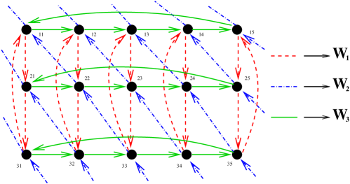
Figure 4: The quiver diagram for the orbifold $\mathbb{C}^{3}/(\mathbb{Z}_{5}\times\mathbb{Z}_{3})$. Each dot represents a $U(N)$ gauge factor, in double index notation. The red dashed lines correspond to chiral multiplets belonging to ${\bf W}_{1}$ , the blue lines to chiral multiplets belonging to ${\bf W}_{2}$ and green ones to chiral multiplets belonging to ${\bf W}_{3}$. Arrows go from fundamental to anti-fundamental representations.

References

- [1] D. Berenstein, J. M. Maldacena, and H. Nastase, “Strings in flat space and pp waves from N=4 super Yang–Mills,” JHEP 04 (2002) 013, hep-th/0202021.
- [2] C. Kristjansen, J. Plefka, G. W. Semenoff, and M. Staudacher, “A new double-scaling limit of N=4 super Yang–Mills theory and pp-wave strings,” hep-th/0205033.
- [3] N. R. Constable et al., “Pp-wave string interactions from perturbative Yang–Mills theory,” JHEP 07 (2002) 017, hep-th/0205089.
- [4] M. Blau, J. Figueroa-O’Farrill, C. Hull, and G. Papadopoulos, “A new maximally supersymmetric background of IIB superstring theory,” JHEP 01 (2002) 047, hep-th/0110242.
- [5] J. Michelson, “(Twisted) toroidal compactification of pp-waves,” hep-th/0203140.
- [6] R. Penrose, “Any space-time has a plane wave as a limit,” in Differential geometry and relativity, Reidel, Dordrecht (1976) 271–275.
- [7] R. Güven, “Plane wave limits and T-duality,” Phys. Lett. B482 (2000) 255–263, hep-th/0005061.
- [8] M. Blau, J. Figueroa-O’Farrill, and G. Papadopoulos, “Penrose limits, supergravity and brane dynamics,” hep-th/0202111.
- [9] S. Kachru and E. Silverstein, “4d conformal theories and strings on orbifolds,” Phys. Rev. Lett. 80 (1998) 4855–4858, hep-th/9802183.
- [10] N. Itzhaki, I. R. Klebanov, and S. Mukhi, “Pp wave limit and enhanced supersymmetry in gauge theories,” JHEP 03 (2002) 048, hep-th/0202153.
- [11] J. Gomis and H. Ooguri, “Penrose limit of N=1 gauge theories,” Nucl. Phys. B635 (2002) 106–126, hep-th/0202157.
- [12] M. Alishahiha and M. M. Sheikh-Jabbari, “The pp-wave limits of orbifolded ,” Phys. Lett. B535 (2002) 328–336, hep-th/0203018.
- [13] N.-W. Kim, A. Pankiewicz, S.-J. Rey, and S. Theisen, “Superstring on pp-wave orbifold from large- quiver gauge theory,” Eur. Phys. J. C25 (2002) 327–332, hep-th/0203080.
- [14] T. Takayanagi and S. Terashima, “Strings on orbifolded pp-waves,” JHEP 06 (2002) 036, hep-th/0203093.
- [15] E. Floratos and A. Kehagias, “Penrose limits of orbifolds and orientifolds,” JHEP 07 (2002) 031, hep-th/0203134.
- [16] S. Mukhi, M. Rangamani, and E. Verlinde, “Strings from quivers, membranes from moose,” JHEP 05 (2002) 023, hep-th/0204147.
- [17] M. Alishahiha and M. M. Sheikh-Jabbari, “Strings in pp-waves and worldsheet deconstruction,” Phys. Lett. B538 (2002) 180–188, hep-th/0204174.
- [18] K. Oh and R. Tatar, “Orbifolds, Penrose limits and supersymmetry enhancement,” hep-th/0205067.
- [19] S. G. Naculich, H. J. Schnitzer, and N. Wyllard, “Pp-wave limits and orientifolds,” hep-th/0206094.
- [20] T. Banks, W. Fischler, S. H. Shenker, and L. Susskind, “M theory as a matrix model: A conjecture,” Phys. Rev. D55 (1997) 5112–5128, hep-th/9610043.
- [21] A. Sen, “D0-branes on and matrix theory,” Adv. Theor. Math. Phys. 2 (1998) 51–59, hep-th/9709220.
- [22] N. Seiberg, “Why is the matrix model correct?,” Phys. Rev. Lett. 79 (1997) 3577–3580, hep-th/9710009.
- [23] L. Motl, “Proposals on nonperturbative superstring interactions,” hep-th/9701025.
- [24] T. Banks and N. Seiberg, “Strings from matrices,” Nucl. Phys. B497 (1997) 41–55, hep-th/9702187.
- [25] R. Dijkgraaf, E. Verlinde, and H. Verlinde, “Matrix string theory,” Nucl. Phys. B500 (1997) 43–61, hep-th/9703030.
- [26] R. Gopakumar, “String interactions in pp-waves,” hep-th/0205174.
- [27] K. Sugiyama and K. Yoshida, “Type IIA string and matrix string on pp-wave,” hep-th/0208029.
- [28] G. Bonelli, “Matrix strings in pp-wave backgrounds from deformed super Yang–Mills theory,” JHEP 08 (2002) 022, hep-th/0205213.
- [29] H. Verlinde, “Bits, matrices and ,” hep-th/0206059.
- [30] M. R. Douglas and G. W. Moore, “D-branes, quivers, and ALE instantons,” hep-th/9603167.
- [31] M. R. Douglas, B. R. Greene, and D. R. Morrison, “Orbifold resolution by D-branes,” Nucl. Phys. B506 (1997) 84–106, hep-th/9704151.
- [32] A. E. Lawrence, N. Nekrasov, and C. Vafa, “On conformal field theories in four dimensions,” Nucl. Phys. B533 (1998) 199–209, hep-th/9803015.
- [33] M. Alishahiha, M. A. Ganjali, A. Ghodsi, and S. Parvizi, “On type IIA string theory on the pp-wave background,” hep-th/0207037.
- [34] R. R. Metsaev and A. A. Tseytlin, “Exactly solvable model of superstring in plane wave Ramond-Ramond background,” Phys. Rev. D65 (2002) 126004, hep-th/0202109.
- [35] R. R. Metsaev, “Type IIB Green-Schwarz superstring in plane wave Ramond- Ramond background,” Nucl. Phys. B625 (2002) 70–96, hep-th/0112044.
- [36] D. J. Gross, A. Mikhailov, and R. Roiban, “Operators with large R charge in N=4 Yang–Mills theory,” hep-th/0205066.
- [37] A. Santambrogio and D. Zanon, “Exact anomalous dimensions of N=4 Yang–Mills operators with large R charge,” hep-th/0206079.
- [38] Y. Oz and T. Sakai, “Exact anomalous dimensions for N=2 ADE SCFTs,” hep-th/0208078.
- [39] U. Gursoy, “Vector operators in the BMN correspondence,” hep-th/0208041.
- [40] D. Berenstein and H. Nastase, “On lightcone string field theory from super Yang–Mills and holography,” hep-th/0205048.
- [41] M. Spradlin and A. Volovich, “Superstring interactions in a pp-wave background,” hep-th/0204146.
- [42] Y.-J. Kiem, Y.-B. Kim, S.-M. Lee, and J.-M. Park, “Pp-wave/Yang–Mills correspondence: An explicit check,” Nucl. Phys. B642 (2002) 389–404, hep-th/0205279.
- [43] M.-X. Huang, “Three point functions of N=4 super Yang–Mills from light cone string field theory in pp-wave,” Phys. Lett. B542 (2002) 255–260, hep-th/0205311.
- [44] C.-S. Chu, V. V. Khoze, and G. Travaglini, “Three-point functions in N=4 Yang–Mills theory and pp-waves,” JHEP 06 (2002) 011, hep-th/0206005.
- [45] P. Lee, S. Moriyama, and J.-W. Park, “Cubic interactions in pp-wave light cone string field theory,” hep-th/0206065.
- [46] M. Spradlin and A. Volovich, “Superstring interactions in a pp-wave background. II,” hep-th/0206073.
- [47] C.-S. Chu, V. V. Khoze, and G. Travaglini, “pp-wave string interactions from -point correlators of BMN operators,” hep-th/0206167.
- [48] I. R. Klebanov, M. Spradlin, and A. Volovich, “New effects in gauge theory from pp-wave superstrings,” hep-th/0206221.
- [49] M.-X. Huang, “String interactions in pp-wave from N=4 super Yang–Mills,” hep-th/0206248.
- [50] C.-S. Chu, V. V. Khoze, M. Petrini, R. Russo, and A. Tanzini, “A note on string interaction on the pp-wave background,” hep-th/0208148.
- [51] N. Beisert, C. Kristjansen, J. Plefka, G. W. Semenoff, and M. Staudacher, “BMN correlators and operator mixing in N=4 super Yang–Mills theory,” hep-th/0208178.
- [52] D. J. Gross, A. Mikhailov, and R. Roiban, “A calculation of the plane wave string hamiltonian from N=4 super-Yang–Mills theory,” hep-th/0208231.
- [53] J.-G. Zhou, “Pp-wave string interactions from string bit model,” hep-th/0208232.
- [54] N. R. Constable, D. Z. Freedman, M. Headrick, and S. Minwalla, “Operator mixing and the BMN correspondence,” hep-th/0209002.
- [55] P. Lee, S. Moriyama, and J.-W. Park, “A note on cubic interactions in pp-wave light cone string field theory,” hep-th/0209011.
- [56] E. Kiritsis and B. Pioline, “Strings in homogeneous gravitational waves and null holography,” JHEP 08 (2002) 048, hep-th/0204004.
- [57] M. Bertolini, P. Di Vecchia, and R. Marotta, “N=2 four-dimensional gauge theories from fractional branes,” hep-th/0112195.
- [58] C. V. Johnson and R. C. Myers, “Aspects of type IIB theory on ALE spaces,” Phys. Rev. D55 (1997) 6382–6393, hep-th/9610140.
- [59] M. Bershadsky, Z. Kakushadze, and C. Vafa, “String expansion as large expansion of gauge theories,” Nucl. Phys. B523 (1998) 59–72, hep-th/9803076.
- [60] M. Bershadsky and A. Johansen, “Large limit of orbifold field theories,” Nucl. Phys. B536 (1998) 141–148, hep-th/9803249.
- [61] A. Hanany and A. M. Uranga, “Brane boxes and branes on singularities,” JHEP 05 (1998) 013, hep-th/9805139.