MSSM parameters from supergravity backgrounds

Abstract

We find the parameters of the MSSM in terms of bulk supergravity fields for the D-brane model of Berenstein, Jejjala and Leigh (hep-ph/0105042). The model consists of a D3-brane at the singularity of a non-abelian orbifold $\Delta_{27}$, which gives the particles of the Supersymmetric Standard Model. We compute the action for the D-brane fields in the presence of both supersymmetric and supersymmetry breaking background fluxes. We get quark, lepton, gaugino, Higgsino, scalar partners and Higgs boson masses as well as soft trilinear couplings as functions of the background fields. This work develops a framework for connecting MSSM phenomenology to brane compactifications.

I Introduction

The Standard Model of Particle Physics has passed stringent quantitative experimental tests. This means that if string theory is the underlying theory, it should contain as a low energy limit the Standard Model. The viewpoint on how to embed the Standard Model in string theory has changed over the past five years. The heterotic string no longer has a monopoly, yielding its place to (heterotic) M-theory, type I and type II strings.

Semirealistic models have been constructed using different types of compactifications (see SM95 and references therein). Another approach, one of the most popular nowadays, arises after the realization that gauge fields in type I theory live on the world-volume of a Dp-brane (see TASI for review), while gravity fields are realized as closed strings living in the bulk. The hierarchy between the Planck scale and the weak scale is explained by large extra dimensions Dimopoulos or a warped space RS ; GKP ; DWG . The string scale is no longer tied to the Planck scale, and can be as low as the experimental bound of 1 TeV.

By combining groups of rotated branes and antibranes, extended in 4 dimensions and wrapped in the others, with or without orbifolds, several models with the matter content of the Standard Model have been built SM>95 . Since the gauge group on a set of $N$ D-branes is $SU(N)$, these models contain usually sets of branes in groups of 2 or 3 to give the Standard Model gauge group. A model first proposed, among various others, by Aldazabal, Ibañez, Quevedo and Uranga AIQU , and taken up by Berenstein, Jejjala and Leigh a year ago Berenstein , stands out for its simplicity: it contains just one D3-brane. The way to get the Standard Model is by orbifolding the 6-dimensional space by a non-abelian subgroup of $SU(3)$ ($\Delta_{27}$), thus preserving ${\mathcal{N}}=1$ supersymmetry. This model realizes all the particles of the Supersymmetric Standard Model (SSM), with six Higgs doublets and right handed neutrinos.

D-brane fields interact with bulk fields, modifying their masses and couplings. The precise result of this interaction for the models built so far has not been determined yet, to our knowledge. In this paper, we will get the Lagrangian for the Standard Model particles in the presence of background fluxes, for the model built in Berenstein . In consequence, we will get all the parameters of the softly broken SSM in terms of the (supersymmetry breaking) background fluxes, thus building the bridge between MSSM phenomenology and string configurations in background fluxes.

The paper is organized as follows. In Section II, we present the model of Berenstein, Jejjala and Leigh that leads to the particle content of the SSM. In Section III we find the background that survives the orbifold projection, preserves Lorentz invariance on the world-volume and solves the equations of motion, as a power series in the distance to the orbifold point. To get the Lagrangian for a D3-brane in the $\Delta_{27}$ orbifold, we start with the non-abelian Dirac-Born-Infeld and Wess-Zumino bosonic actions in the background found in Section II. For the fermionic action, we will use the abelian one for a D3-brane computed in Grana , and find any non-abelian additional terms with the help of the non-abelian action for D0-branes Taylor2 . All this is done in Section III. In Section IV, we find the parameters of the MSSM in terms of background fluxes, and we state our conclusions in Section V. Appendix A shows the details of the non-abelian group by which the orthogonal directions are orbifolded, and explains how to get the matter content for a D-brane at the orbifold point.

II The Model

If we orbifold the space orthogonal to a D3-brane by a discrete subgroup $\Gamma$ of $SU(3)$, we get on the brane an ${\mathcal{N}}=1$, $\Pi_{a=1}^{r}U(N_{a})$ gauge theory, where $N_{a}$ are the dimensions of the irreducible representations of $\Gamma$, with chiral multiplets transforming as $(N_{a},\overline{N}_{b})$ Lawrence . It was shown in Berenstein that when $\Gamma$ is the non-abelian group $\Delta_{27}$, the matter obtained from keeping states invariant under the orbifold projection resembles very closely that of the standard model, with three quark and lepton generations, neutrino singlets and six Higgs doublets.

The miracle works as follows Greene ; Muto ; Hanany : to find states invariant under the orbifold projection, we have to consider the D3-brane and all of its images, making a total of $|\Gamma|$ ($|\Gamma|$ is the order -number of elements- of the group) D3-branes. In the case of the group $\Delta_{27}$, there are $27$ D3-branes to start with, and the original world-volume theory is an ${\mathcal{N}}=1$, $U(27)$ gauge theory, with a $U(27)$ vector multiplet $V$, made out of the gauge fields and the gauginos $\lambda$, and three chiral multiplets $\Phi^{i}$ composed by the complex scalars $\phi^{i}$, identified with the orthogonal complex coordinates $z^{i}$, and three Weyl fermions $\psi^{i}$, all of them $N\times N$ matrices, transforming in the adjoint representation. Projecting onto $\Gamma$ invariant states means satisfying

$$R_{reg}VR_{reg}^{-1}=V$$ (1)

$$(R_{3})_{ij}R_{reg}\Phi^{j}R_{reg}^{-1}=\Phi^{i}$$ (2)

where $R_{reg}$ is the $N\times N$ regular representation acting on the Chan-Paton index, and $R_{3}$ is the 3-dimensional defining representation that acts on the space-time index $i$. Any representation can be decomposed into a sum of irreducible representations $R^{a}$. For the regular representation, the decompositions works as follows

$$R_{reg}=\oplus_{a=1}^{r}N_{a}R^{a}$$ (3)

where $N_{a}=dimR^{a}$, i.e. each irreducible representation $R^{a}$ occurs $N_{a}$ times in the regular representation. The regular representation then has the form

$$R_{reg}=\pmatrix{R^{1}\otimes 1_{N_{1}}&0&...&0\cr 0&R^{2}\otimes 1_{N_{2}}&...&0\cr\vdots&\vdots&\ddots&\vdots\cr 0&0&...&R^{r}\otimes 1_{N_{r}}}$$ (4)

where $R^{a}\otimes 1_{N_{a}}$ is the $N_{a}\times N_{a}$ matrix with $N_{a}$ copies of $R^{a}$

$$R^{a}\otimes 1_{N_{a}}=\pmatrix{R^{a}&0&...&0\cr 0&R^{a}&...&0\cr\vdots&\vdots&\ddots&\vdots\cr 0&0&...&R^{a}}$$ (6)

From Eq.(1) we get that the gauge symmetry is

$$\prod_{a=1}^{r}U(N_{a})$$ (8)

The group $\Delta_{27}$ has two 3-dimensional and nine 1-dimensional representations. Thus the gauge theory on the D3-brane is a $U(3)^{2}\times U(1)^{9}$. The first of these $U(3)$’s will be identified with color, and the second one, combined with some of the $U(1)$’s, and after breaking part of the symmetry, with $SU(2)\times U(1)$ of the electroweak interactions. At the weak scale only the hypercharge plus two other $U(1)$ symmetries will survive. The condition (2) tells us the number of chiral fields $n^{3}_{ab}$ transforming in the $(N_{a},\overline{N}_{b})$, by decomposing the product of the defining and each irreducible representation into irreducible representations in the following way:

$$R_{3}\otimes R^{a}=\oplus_{b=1}^{r}n^{3}_{ab}R^{b}.$$ (9)

It is shown in the Appendix how to get the numbers $n^{3}_{ab}$ from the table of characters of a group. In the case of the group $\Delta_{27}$, we get 3 chiral multiplets transforming as ${\cal Q}_{i}=(3,\overline{3},0)$ of $U(3)_{c}\times U(3)_{w}\times U(1)^{a}$, and one multiplet for each $U(1)$ group, transforming as ${\cal L}_{a}=(1,3,-_{a})$ and $\overline{{\cal Q}}_{a}=(\bar{3},1,+_{a})$, using the notation of Berenstein . Gauge couplings are given by

$$\tau_{a}=\frac{N_{a}\tau}{|\Gamma|}$$ (10)

The quiver of the theory is shown in Figure 1.

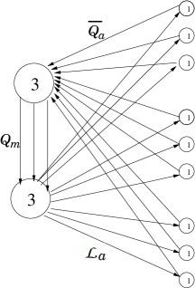
Figure 1: Quiver diagram for the group $\Delta_{27}$

As a first step, Berenstein, Jejjala and Leigh add Fayet-Iliopoulos parameters for three of the $U(1)$’s, enabling a supersymmetry preserving vacuum expectation value for three scalars in the chiral multiplet ${\cal L}_{a}$. This breaks $U(3)_{w}\times U(1)^{3}$ into $SU(2)_{w}\times U(1)_{0}$. Then all fields transforming in the fundamental representation of $U(3)_{w}$ get split into an $SU(2)$ doublet and an $SU(2)$ singlet. Then, we can find all the supersymmetric Standard Model particles in the spectrum of this theory as follows:

$${\cal Q}_{m} \rightarrow Q_{m}\ ,\ q_{m}\qquad\qquad \bar{{\cal Q}}_{1,m}\equiv\bar{q}_{m}$$

$${\cal L}_{1,m} \rightarrow L_{m}\ ,\ g_{m}\qquad\qquad \bar{{\cal Q}}_{2,m}\equiv\bar{u}_{m}$$ (11)

$${\cal L}_{2,m} \rightarrow H_{m}\ ,\ \bar{e}_{m}\qquad\qquad \bar{{\cal Q}}_{3,m}\equiv\bar{d}_{m}$$

$${\cal L}_{3,m} \rightarrow{\overline{H}}_{m}\ ,\ \bar{\nu}_{m}\qquad\qquad$$

where the fields on the left are those that transform as a $3$ of $U(3)_{w}$, and we give their decomposition into $SU(2)_{w}$ doublets and singlets. The index $a$ has been decomposed into a pair $l,m$, and the fields charged under the three $U(1)$’s of the form “$1,m$” (called $g_{m}$ in Eq.(II)) are those that get VEVs.

As we can see, we get all of the fields of the Standard Model. The index $m$ is a generation index, so we get three quark generations and three lepton generations, with both $SU(2)_{w}$ doublets and singlets (we get a neutrino singlet), and six Higgs doublet fields. Besides, there are fields not present in the Standard Model, namely $g_{m}$, which get vevs that break one of the $U(3)$’s into $SU(2)_{w}$, and those called $q_{m}$ and $\bar{q}_{m}$, which get mass from the superpotential coming from ${\mathcal{N}}$=4, and can be integrated out.

It is remarkable that with just one D3-brane we can get the matter content of the Standard Model.

III Background

In this Section we are going to immerse the D3-brane in background fluxes. But not any flux survives the orbifold projection, so we will find first those that do survive and also solve the equations of motion. We will find them as a series expansion in $z^{i}$, the complex distance to the orbifold singularity, up to second order.

To preserve Lorentz invariance on the D3-brane, we want the metric to be of the warped form, so in its longitudinal part there can be at most a warp factor multiplying the Minkowski metric. For the remaining directions, we can have any metric component ($dz^{i}dz^{j}$, $d\bar{z}^{i}d\bar{z}^{j}$ and $dz^{i}d\bar{z}^{j}$), as long as they give a metric invariant under the orbifold operations. The rest of the fields (axion-dilaton, 5- and 3-form fluxes) can only be a function of $z^{i}$ and $\bar{z}^{i}$. We will divide the 3-form flux into pieces according to the number of holomorphic and antiholomorphic indexes: (3,0); (0,3); (1,2) and (2,1). It will be convenient to express the (1,2) and (2,1) pieces in terms of a symmetric and an antisymmetric 2-tensor, in the way shown below.

The only possible expansion of these fields compatible with the orbifold are

$$ds^{2} = \left(1+k_{2}z^{i}\bar{z}^{i}\right)\eta_{\mu\nu}dx^{\mu}dx^{\nu}+\left((1+h_{2}z^{k}\bar{z}^{k})\delta_{ij}+l_{2}\bar{z}^{i}z^{j}\right)dz^{i}d\bar{z}^{j}$$

$$+g_{2}\bar{z}^{i}\bar{z}^{j}dz^{i}dz^{j}+g_{2}^{*}z^{i}z^{j}d\bar{z}^{i}d\bar{z}^{j}$$

$$G_{123} = G_{0}+G_{2}z^{i}\bar{z}^{i},\qquad G_{\bar{1}\bar{2}\bar{3}}=G^{\prime}_{0}+G^{\prime}_{2}z^{i}\bar{z}^{i}$$

$$S_{ij} \equiv \frac{1}{2}\left(\epsilon_{ikl}G_{{\bar{k}}{\bar{l}}j}+\epsilon_{jkl}G_{{\bar{k}}{\bar{l}}i}\right)=s_{2}\bar{z}^{i}\bar{z}^{j}\qquad$$

$$S_{\bar{\imath}\bar{\jmath}} \equiv \frac{1}{2}\left(\epsilon_{\bar{\imath}{\bar{k}}{\bar{l}}}G_{kl\bar{\jmath}}+\epsilon_{\bar{\jmath}{\bar{k}}{\bar{l}}}G_{kl\bar{\imath}}\right)=s^{\prime}_{2}z^{i}z^{j}$$

$$A_{ij} \equiv \frac{1}{2}\left(\epsilon_{ikl}G_{\bar{k}\bar{l}j}-\epsilon_{jkl}G_{\bar{k}\bar{l}i}\right)=a_{1}\epsilon_{ijk}z^{k}$$

$$A_{\bar{\imath}\bar{\jmath}} \equiv \frac{1}{2}\left(\epsilon_{\bar{\imath}{\bar{k}}{\bar{l}}}G_{kl\bar{\jmath}}-\epsilon_{\bar{\jmath}{\bar{k}}{\bar{l}}}G_{kl\bar{\imath}}\right)=-a_{1}\epsilon_{\bar{\imath}\bar{\jmath}{\bar{k}}}\bar{z}^{k}$$

$$\tau = \tau_{0}+\tau_{2}z^{i}\bar{z}^{i},\qquad F_{i\bar{\imath}j\bar{\jmath}k}=F_{1}\epsilon_{i\bar{\imath}j\bar{\jmath}k\bar{k}}\bar{z}^{k}$$ (12)

where $k_{2},h_{2},l_{2}$ and $F_{1}$ are real constants, and $g_{2},s_{1},s^{\prime}_{1},a_{1},\tau_{0},\tau_{2},G_{0},G_{2}$ are complex numbers and $\epsilon_{i\bar{\imath}j\bar{\jmath}k\bar{k}}=i$

The fields in Eq.(III), with any value of the constants, satisfy the orbifold projection but not necessarily the equations of motion. In general, the equations of motion give relationships between the constants, as we will show.

The field equations for type IIB supergravity are

$$\bigtriangledown^{m}\left(\frac{i}{2}e^{\phi}\partial_{m}\tau\right) - \frac{1}{2}e^{2\phi}\partial^{m}C\partial_{m}\tau=\frac{g_{s}}{24}G_{mnp}G^{mnp}\,$$

$$\bigtriangledown^{m}G_{mnp} + \frac{i}{2}e^{\phi}\partial^{m}CG_{mnp}=-\frac{i}{2}e^{\phi}\partial^{m}\tau G_{mnp}^{\ast}-\frac{g_{s}}{6}iF_{mnpqr}G^{mqr}\,,$$

$$R_{mn} = \frac{1}{4}e^{2\phi}\partial_{m}\tau\partial_{n}\tau^{\ast}+\frac{1}{4}e^{2\phi}\partial_{m}\tau^{\ast}\partial_{n}\tau+\frac{g_{s}^{2}}{96}F_{mqrst}{F_{n}}^{qrst}$$

$$+\frac{g_{s}}{8}\left({G_{m}}^{pq}G_{npq}^{\ast}+{G_{n}}^{pq}G_{mpq}^{\ast}-\frac{1}{6}g_{mn}G_{pqr}^{\ast}G^{pqr}\right)\,.$$

The Bianchi identities are

$$\partial_{[m}G_{nkl]}+\frac{i}{2}e^{\phi}\partial_{[m}CG_{nkl]}=\frac{i}{2}e^{\phi}\partial_{[m}\tau G^{\ast}_{nkl]},\qquad\partial_{[m}F_{nklpq]}=\frac{5}{48}iG_{[mnk}G^{\ast}_{lpq]}$$ (14)

Inserting the fields (III) in the equations of motion (III) and Bianchi identities (14), we get relationships between the constants appearing in the fields. Solving them requires

$$a_{1} = 0$$ (15)

$$12F_{1} = |G_{0}|^{2}-|G^{\prime}_{0}|^{2}$$ (16)

$$\tau_{2} = -\frac{i}{3}G_{0}G^{\prime}_{0}$$ (17)

$$24k_{2} = g_{s}\left(|G_{0}|^{2}+|G^{\prime}_{0}|^{2}\right)$$ (18)

$$k_{2} = \frac{1}{5}\left(8Reg_{2}+l_{2}-5l_{2}\right)$$ (19)

$$F_{1}G^{\prime}_{0}g_{s} = -\frac{i}{2}g_{s}\left(Re\tau_{2}G^{\prime}_{0}+\tau_{2}(G^{\prime}_{0})^{\ast}\right)+8g_{2}G^{\prime}_{0}-4s_{2}-G^{\prime}_{2}$$ (20)

$$F_{1}G_{0}g_{s} = -\frac{i}{2}g_{s}\left(Re\tau_{2}G_{0}+\tau_{2}(G_{0})^{\ast}\right)+8g^{\ast}_{2}G_{0}-4s^{\prime}_{2}-G_{2}$$ (21)

$$0 = \frac{i}{2}g_{s}\left(Re\tau_{2}G^{\prime}_{0}-\tau_{2}(G^{\prime}_{0})^{\ast}\right)+2s_{2}+G^{\prime}_{2}$$ (22)

$$0 = \frac{i}{2}g_{s}\left(Re\tau_{2}G_{0}-\tau_{2}(G_{0})^{\ast}\right)+2s^{\prime}_{2}+G_{2}\$$ (23)

where $g_{s}=1/Im\tau_{0}$.

Any configuration of the form (III) satisfying Eqs.(15-23) is a consistent background.

At zeroth order, the free parameters are the axion-dilaton $\tau_{0}$, and the (3,0) and (0,3) constant 3-form flux pieces $G_{0}$ and $G^{\prime}_{0}$. $G_{0}$ and $G^{\prime}_{0}$ determine the first order parameter $F_{1}$ in the 5-form flux, as can be seen in Eq.(16), and the second order $\tau_{2}$ and $k_{2}$ in the dilaton and longitudinal metric, respectively, as shown in Eqs.(17) and (18). The remaining six second order parameters ($G_{2},g_{2},s_{2},s^{\prime}_{2},l_{2}$ and $h_{2}$) are constrained by five equations, Eqs.(19)-(23) so there is some freedom to play with.

The four supersymmetries preserved by the orbifold are the same as those studied in GP ; Gubser , where it was shown that the (3,0); (0,3) and symmetric (1,2) pieces of the 3-form flux, as well as a non-vanishing antiholomorphic derivative of the dilaton, break supersymmetry. Then, a vacuum expectation value for $G_{0}$, $G^{\prime}_{0}$, $G_{2}$, $G^{\prime}_{2}$, $s_{2}$ and $\tau_{2}$ break supersymmetry. As we will see, $G_{0}$ will generate gaugino masses and soft trilinear A-terms. $s_{2}$ will appear in lepton masses and in the $\mu$-term, and $F_{1},k_{2}$ and $\tau_{2}$ will combine to give masses to the scalar partners.

IV Action

We wish to find the non-abelian action corresponding to 27 D3-branes at the orbifold point, in the background found in the previous Section. The bosonic part of action is known, it is the non-abelian Born Infeld and Wess Zumino actions Myers ; Taylor1 , that we can trust up to terms of order $F^{4}$. This is enough for us, since we just want the $F$-independent terms. In the case of the fermionic action, the non-abelian version of it is not known yet. For a flat background, we know the action will be that of ${\mathcal{N}}=1$, $U(27)$ super-Yang Mills with the superpotential $W=Tr\left([\Xi^{i},\Xi^{j}]\Xi^{k}\right)$ ($\Xi^{i}$ is the chiral superfield containing $\Phi^{i}$ and $\psi^{i}$). When nontrivial fluxes are present, the brane-background fermionic couplings for a D3-brane have been found in Grana for just one D3-brane, and these will appear in the non-abelian action with a trace over the gauge indexes. Finally, we will check that there are not any additional couplings than those already found, using the T-dual of the non-abelian action linear in the background for $N$ D0-branes found from matrix theory in Taylor2 .

Let us start with the bosonic action (we use the notation of Myers ):

$$S= - \mu_{3}\int d^{4}\zeta\,Tr\left(e^{-\phi}\sqrt{-det\left(P\left[E_{\mu\nu}+E_{\mu i}\,(Q^{-1}-\delta)^{ij}E_{j\nu}\right]+2\pi\alpha^{\prime}F_{\mu\nu}\right)det(Q^{i}_{j})}\right)$$ (24)

$$+ \mu_{3}\int Tr\left(P\left[e^{i2\pi\alpha^{\prime}i_{\Phi}i_{\Phi}}\sum C_{(n)}e^{B}\right]e^{2\pi\alpha^{\prime}F}\right)$$

where $P$ is the pull-back of the spacetime fields into the world-volume, defined

$$P\left[E\right]_{\mu\nu}=E_{\mu\nu}+2\pi\alpha^{\prime}E_{i(\mu}D_{\nu)}\Phi^{i}+4\pi^{2}\alpha^{\prime 2}E_{ij}D_{\mu}\Phi^{i}D_{\nu}\Phi^{j},\qquad D_{\mu}\Phi^{i}=\partial_{\mu}\Phi^{i}+i[A_{\mu},\Phi^{i}]$$ (25)

the scalars $\Phi^{i}$ are the orthogonal coordinates $z^{i}$ rescaled by a factor $2\pi\alpha^{\prime}$ as: $\Phi^{i}=\frac{z^{i}}{2\pi\alpha^{\prime}}$, the tensor $E$ and $Q$ are defined

$$E_{\mu\nu}\equiv G_{\mu\nu}+B_{\mu\nu},\qquad Q^{i}_{j}\equiv\delta^{i}_{j}+i2\pi\alpha^{\prime}[\Phi^{i},\Phi^{k}]E_{kj}$$ (26)

and $i_{\Phi}$ denotes the interior product by $\Phi$

$$i_{\Phi}i_{\Phi}C_{(2)}=\Phi^{j}\Phi^{i}C_{ij}.$$ (27)

Inserting the background (III), and expanding the square root in the Dirac-Born-Infeld action, we get, up to terms of dimension four,

$${\mathcal{L}}=\frac{1}{g_{s}}\,Tr\left(\frac{1}{2}\partial_{\mu}\Phi^{i}\partial^{\mu}\Phi^{\bar{\imath}}+(-2k_{2}-g_{s}F_{1}-g_{s}Im\tau_{2})\,\Phi^{i}\Phi^{\bar{\imath}}\right.$$

$$-\frac{1}{3}G_{0}\epsilon_{ijk}\Phi^{i}\Phi^{j}\Phi^{k}-\frac{1}{3}G^{\prime}_{0}\epsilon_{\bar{\imath}\bar{\jmath}\bar{k}}\Phi^{\bar{\imath}}\Phi^{\bar{\jmath}}\Phi^{\bar{k}}\left.-\frac{1}{2}[\Phi^{j},\Phi^{(i}][\Phi^{\bar{\imath})},\Phi^{\bar{\jmath}}]\right)$$ (28)

For the fermionic action, we first recall the abelian one obtained from the kappa-symmetric action Grana :

$${\mathcal{L}}=-\frac{1}{2}\bar{\psi}^{\bar{\imath}}\Gamma^{\mu}D_{\mu}\psi^{i}-\frac{1}{2}\bar{\lambda}\Gamma^{\mu}D_{\mu}\lambda+\frac{1}{48}\psi^{i}\psi^{j}S_{ij}+\frac{1}{48}\lambda\lambda G_{123}+\frac{1}{96}\epsilon_{ijk}\psi^{i}\lambda A_{\bar{\jmath}{\bar{k}}}$$ (29)

where $\psi^{i}$ are the superpartners of $\Phi^{i}$, and $\lambda$ is the gaugino

The non-abelian action will have the terms in Eq.(29) traced over the gauge indexes, plus those known to appear in the flat space action, that come from ${\mathcal{N}}=4$. Up to dimension five operators, the fermionic non-abelian action is

$${\mathcal{L}}=Tr\left(-\frac{1}{2}\bar{\psi}^{\bar{\imath}}\Gamma^{\mu}D_{\mu}\psi^{i}-\frac{1}{2}\bar{\lambda}\Gamma^{\mu}D_{\mu}\lambda+\frac{4\pi^{2}\alpha^{\prime 2}}{48}s_{2}\psi^{i}\Phi^{\bar{\imath}}\psi^{j}\Phi^{\bar{\jmath}}\right.$$

$$\left.+\frac{1}{48}G_{0}\lambda\lambda+\frac{\pi^{2}\alpha^{\prime 2}}{12}G_{2}\lambda\lambda\Phi^{i}\Phi^{\bar{\imath}}+\frac{1}{2g_{s}}\epsilon_{ijk}\psi^{i}\psi^{j}\Phi^{k}+\frac{1}{2}[\psi^{\bar{\imath}},\Phi^{i}]\lambda\right)$$ (30)

The first five terms are the ones that appear in the abelian action (29), applied to the background (III). The last two, that are zero in the abelian case, are those that come from the ${\mathcal{N}}=4$ theory. In particular, the next to the last term in Eq.(IV) comes from the superpotential term $W=Tr\left([\Xi^{i},\Xi^{j}]\Xi^{k}\right)$.

It remains to check that there are no more intrinsically non-abelian terms showing up in curved space, and we will do that with the help of the non-abelian D0-brane action found in Taylor2 . This action was found from matrix theory, and involves the fermionic world-volume coordinate $\Theta$, which is a 10D Majorana-Weyl fermion transforming in the adjoint of the gauge group. This fermion, when splitting the ${\bf\overline{16}}$ of $SO(9,1)$ into $({\bf\bar{2}},{\bf 4})+({\bf 2},{\bf\bar{4}})$ of $SO(3,1)\otimes SO(6)$, gives the three fermions in the chiral multiplet $\psi^{i}$ and the gaugino $\lambda$.

The terms that we are interested in would involve a commutator of a scalar field $\Phi$ and the fermion $\Theta$ (and another power of $\Theta$), or the commutator of two $\Phi$’s together with a fermion bilinear. From the results shown in Taylor2 , we can see that terms with a commutator of $\Phi$ and $\Theta$ appear in the 11-dimensional stress tensor $T^{ij}$, membrane currents $J^{ijk}$, $J^{+-i}$ and 5-brane current $M^{+-ijkl}$, where $+$ and $-$ are light cone coordinates, in the form

$$T^{ij} \propto {\overline{\Theta}}\Gamma^{i}[\Phi^{j},\Theta]+{\overline{\Theta}}\Gamma^{j}[\Phi^{i},\Theta]+...\qquad M^{+-ijkl}\propto{\overline{\Theta}}\Gamma^{[ijk}[\Phi^{l]},\Theta]+...$$

$$J^{ijk} \propto {\overline{\Theta}}\Gamma^{0[ik}[\Phi^{k]},\Theta]+...\qquad\quad\qquad\quad\quad\quad J^{+-i}\propto{\overline{\Theta}}\Gamma^{0}[\Phi^{i},\Theta]+...$$ (31)

where “$+...$” indicates terms of a different structure. These currents couple to $h_{ij}$, $C_{ijk}$, $B_{0i}$ and $C_{0ijkl}$ in the IIA theory, as follows:

$${\cal L}\propto h_{ij}T^{ij}+C_{ijk}J^{ijk}+3B_{0i}J^{+-i}+6\,C_{0ijkl}M^{+-ijkl}+...$$ (32)

Performing T-duality in 3 directions to get the D3-brane couplings, we get couplings to $h_{ij}$, $h_{\mu\nu}$, $C_{\mu i}$, $C_{\mu\nu ij}$,$C_{\mu\nu\rho ijk}$, $B_{0i}$ and $C_{\mu\nu\lambda\rho ijkl}$, where Greek letters indicate directions along the D3-brane. These are either 0 or second order in $\Phi$, giving higher order terms.

Terms of the form $[\Phi^{i},\Phi^{j}]\Theta^{2}$ appear in the first moments of the currents, which couple to one derivative of the background fields (i.e. couple to the field strengths and not the potentials). Since $[\Phi^{i},\Phi^{j}]\Theta^{2}$ is already dimension 5, we need just to look at the possibility of a coupling of this form to $G_{ijk}$ or $G_{\bar{\imath}\bar{\jmath}\bar{k}}$, the only constant field strengths. The T duals of these couple to $J^{\pm ij(k)}$ and $M^{-ij\mu\nu\lambda(k)}$, in the form

$${\cal L}\propto-2\partial_{k}C_{ij\mu\nu\lambda}M^{-ij\mu\nu\lambda(k)}+\partial_{k}B_{ij}\left(J^{+ij(k)}-J^{-ij(k)}\right).$$ (33)

It can be checked from the original M-theory calculation done in TaylorM that these moments of the currents do not contain such $[\Phi^{i},\Phi^{j}]\Theta^{2}$ terms. So, for our background, there are not, up to dimension 5, any other intrinsically non-abelian terms than those already present in flat space, so the actions (IV) and (IV) build the full non-abelian action for a D3-brane in the background fluxes of Eq.(III).

A couple of comments regarding the action are in order: the quadratic and cubic terms in the bosonic part of the action (Eq.(IV)) break supersymmetry explicitly, and they come from fluxes that break supersymmetry in the bulk. On the contrary, the quartic piece in the bosonic action is SUSY preserving, as it comes from the superpotential $W=Tr\left([\Xi^{i},\Xi^{j}]\Xi^{k}\right)$. In the fermionic action (Eq.(IV)), the terms proportional to $s_{2}$, $G_{0}$ and $G_{2}$ break supersymmetry (the first one because it cannot be of the form $\psi^{i}\psi^{j}\partial^{2}W/\partial_{i}\Phi\partial_{j}\Phi$, since $W$ cannot depend on $\Phi^{\bar{\imath}}$), and also come from supersymmetry breaking bulk supergravity fields. The last two terms preserve supersymmetry, the first one comes from the superpotential written above, and the last one from the Kahler part of the Lagrangian. The second comment is that fermions couple only to $S_{ij},G_{ijk}$ and $A_{\bar{\imath}\bar{\jmath}}$, as can be seen from Eq.(29). These pieces of the 3-form flux vanish in no-scale structure solutions NS .

As far as the bosonic action, the scalar mass term also vanishes in no scale structure models, as we will see below. The $(0,3)$ piece of the 3-form flux, which breaks supersymmetry but is present in no-scale structure solutions, appears in the bosonic action, but in a term that is intrinsically non-abelian, so it is not present in brane-world models with just one D-brane. The vanishing of tree level masses coming from supersymmetry breaking fluxes is a general prediction of no-scale structure models NSNM ; DWG . The cosmological constant vanishes for these models, even though supersymmetry is broken in the bulk.

Now that we have the whole non-abelian action, we can write it in terms of the fields in irreducible representations, shown in Figure 1. Let us start with the bosonic part. Each term where an index $i$ is contracted with an $\bar{\imath}$, like the mass term in Eq.(IV), gives bilinears of the form

$$Tr\left(\Phi^{i}\Phi^{\bar{\imath}}\right)\rightarrow\sum_{lm}{\tilde{\cal Q}}^{\dagger}_{l}{\tilde{\cal Q}}_{m}+{\tilde{\cal L}}^{\dagger}_{a}{\tilde{\cal L}}_{a}+{\tilde{\bar{\cal Q}}}^{\dagger}_{a}{\tilde{\bar{\cal Q}}}_{a}$$ (34)

Each term on the r.h.s. of this equation is multiplied by a constant. These same constants appear also in the kinetic terms, so we can get rid of them by renormalizing the fields.

A trilinear term of the form $\Phi^{i}\Phi^{j}\Phi^{k}$, as in the third term in Eq.(IV), gives

$$Tr\left(\Phi^{i}\Phi^{j}\Phi^{k}\right)\rightarrow\sum_{la}\lambda_{la}{\tilde{\cal Q}}_{l}{\tilde{\cal L}}_{a}{\tilde{\bar{\cal Q}}}_{a}$$ (35)

The way to understand this, and get the value of the coefficients $\lambda_{la}$, is the following: each $\Phi^{i}$ on the l.h.s. transforming originally in the adjoint of $U(27)$, corresponds, in the orbifolded theory, to a bifundamental $\phi^{a{\bar{b}}}$, a scalar field that goes from node $a$ to node $b$ in the quiver diagram of Figure 1. This identification has to be accompanied with a Clebsh-Gordan coefficient $Y^{i}_{a{\bar{b}}}$ coming from the projection $R_{3}\otimes R^{a}\rightarrow R^{b}$ as in Eq.(56). A product of three $\Phi$’s then gives

$$Tr\left(\Phi^{i}\Phi^{j}\Phi^{k}\right)\rightarrow Y^{i}_{a{\bar{b}}}Y^{j}_{b{\bar{c}}}Y^{k}_{c{\bar{a}}}\,\phi^{a{\bar{b}}}\phi^{b{\bar{c}}}\phi^{c{\bar{a}}}$$ (36)

So the trilinear coupling appearing in the third term of Eq.(IV) is

$$Tr\left(G_{ijk}\Phi^{i}\Phi^{j}\Phi^{k}\right)\rightarrow G_{0}\sum_{la}\lambda_{la}{\tilde{\cal Q}}_{l}{\tilde{\cal L}}_{a}{\tilde{\bar{\cal Q}}}_{a}$$ (37)

where

$$\lambda_{la}=\epsilon_{ijk}Y^{i}_{(3_{c}{\bar{3}}_{w})_{l}}Y^{j}_{(3_{w}{\bar{1}}^{a})}Y^{k}_{(1^{a}{\bar{3}}_{c})}$$ (38)

and we have identified $a,b$ and $c$ in Eq.(36) with $U(3)_{c},U(3)_{w}$ and $U(1)^{a}$ respectively.

The same can be done with the quartic terms, containing contractions $i\bar{\imath}j\bar{\jmath}$, which will give terms of the form

$$Tr\left(\Phi^{j}\Phi^{(i}\Phi^{\bar{\imath})}\Phi^{\bar{\jmath}}+h.c.\right) \rightarrow\sum_{lma}\alpha_{lma}{\tilde{\cal Q}}_{l}{\tilde{\cal L}}_{a}{\tilde{\cal L}}^{\dagger}_{a}{\tilde{\cal Q}}^{\dagger}_{m}+\sum_{ab}\beta_{ab}{\tilde{\cal L}}_{a}{\tilde{\overline{\cal Q}}}_{a}{\tilde{\overline{\cal Q}}}^{\dagger}_{b}{\tilde{\cal L}}^{\dagger}_{b}+\sum_{abl}\gamma_{alm}{\tilde{\overline{\cal Q}}}_{a}{\tilde{\cal Q}}_{l}{\tilde{\cal Q}}^{\dagger}_{m}{\tilde{\overline{\cal Q}}}^{\dagger}_{a}$$ (39)

$$+ \sum_{lmno}\eta_{lmno}{\tilde{\cal Q}}_{l}{\tilde{\cal Q}}^{\dagger}_{m}{\tilde{\cal Q}}_{n}{\tilde{\cal Q}}^{\dagger}_{o}+\sum_{ab}\rho_{ab}{\tilde{\cal L}}^{\dagger}_{a}{\tilde{\cal L}}_{b}{\tilde{\cal L}}^{\dagger}_{b}{\tilde{\cal L}}_{a}+\sum_{ab}\nu_{ab}{\tilde{\overline{\cal Q}}}_{a}{\tilde{\overline{\cal Q}}}^{\dagger}_{b}{\tilde{\overline{\cal Q}}}_{b}{\tilde{\overline{\cal Q}}}^{\dagger}_{a}$$

where, for example, $\alpha_{lma}$ can be obtained from the Clebsh-Gordan coefficients as

$$\alpha_{lma}=\sum_{ij}Y^{j}_{(3_{c}{\bar{3}}_{w})_{l}}Y^{i}_{(3_{c}{\bar{1}}^{a})}Y^{\bar{\imath}}_{(1^{a}{\bar{3}}_{w})}Y^{\bar{\jmath}}_{(3_{w}{\bar{3}}_{c})_{m}}$$ (40)

and equivalently for the rest of the coefficients. After breaking $U(3)_{w}\times U(1)^{3}$ to $SU(2)_{w}\times U(1)_{0}$, we get all possible quartic terms involving either zero, two or four $SU(2)$ doublets contracted among them.

V Masses and Couplings

From the fermionic and bosonic actions (IV) and (IV), once decomposed into the fields that furnish irreducible representations of the orbifold group (Eqs.(34), (37) and (39)), we get masses for all the scalars, trilinear A-terms, lepton Yukawa couplings and gaugino masses. Let us analyze them in detail, starting with the fermionic terms.

The term $\psi^{i}\psi^{j}\Phi^{k}$ in Eq.(IV), independent of the fluxes, gives quark Yukawa couplings of the form

$$Tr\left(\epsilon_{ijk}\psi^{i}\psi^{j}\Phi^{k}\right)\rightarrow\sum_{lm}\left(a_{lm}Q_{l}\tilde{H}_{m}{\bar{u}}_{m}+b_{lm}Q_{l}\tilde{\bar{H}}_{m}\bar{d}_{m}\right)$$ (41)

where $a_{lm}$ and $b_{lm}$ can be obtained from the Clebsh-Gordan coefficients

$$a_{lm}=\sum_{ijk}\epsilon_{ijk}Y^{i}_{(3_{c}{\bar{2}}_{w})}Y^{k}_{(2_{w}{\bar{1}}_{2,m})}Y^{j}_{(1_{2,m}{\bar{3}}_{c})}$$ (42)

and similarly for $b_{lm}$ (just change the node $1_{2,m}$ to $1_{3,m}$). We have taken into account the breaking of $U(3)_{w}\times U(1)^{3}$ into $SU(2)_{w}\times U(1)_{0}$.

Up and down quark masses are then given by

$$(m_{u})_{lm}=a_{lm}\langle H_{m}\rangle,\qquad(m_{d})_{lm}=b_{lm}\langle\overline{H}_{,}\rangle$$ (43)

If all $a_{lm}$ and $b_{lm}$ are the same, a hierarchy between generations can be obtained by having a hierarchy of VEVs.

It is worth noting that the symmetries of the orbifold forbid a contribution from the fluxes to quark masses. That contribution would appear if there was a linear term in $S_{ij}$, the symmetric combination of the $(1,2)$ piece of the 3-form flux (see Eq.(29)),which is not compatible with the orbifold projection.

As noted in Berenstein , there are no lepton Yukawa couplings of this form, since the Higgs fields and the leptons belong to the same leg in the quiver of Figure 1. Lepton masses come only at dimension five, from the term of the form $\psi^{i}\Phi^{\bar{\imath}}\psi^{j}\Phi^{\bar{\jmath}}$ in Eq.(IV). Projecting onto the fundamental matter of the orbifold, we get terms of the same form as those in (39), with two scalars replaced by two fermions. The scalar fields that acquire a VEV are ${\tilde{H}}_{m}$, ${\tilde{\overline{H}}}_{m}$ and ${\tilde{g}}_{m}$, the first two are doublets of $SU(2)$ and the last one is a singlet. Then, lepton masses come from terms of the form

$$Tr\left(s_{2}\,\psi^{i}\Phi^{\bar{\imath}}\psi^{j}\Phi^{\bar{\jmath}}\right)\rightarrow\sum_{lm}\left(s_{2}\rho_{lm}L_{l}{\tilde{g}}_{l}^{\dagger}{\overline{e}}_{m}{\tilde{H}}^{\dagger}_{m}+s_{2}\rho^{\prime}_{lm}L_{l}{\tilde{g}}_{l}^{\dagger}{\overline{\nu}}_{m}{\tilde{\overline{H}}}^{\dagger}_{m}\right)$$ (44)

where

$$\rho_{lm}=\sum_{ij}Y^{i}_{(2_{w}{\bar{1}}_{1,l})}Y^{\bar{\imath}}_{(1_{1,l}{\bar{1}}_{0})}Y^{j}_{(1_{0}{\bar{1}}_{1,m})}Y^{\bar{\jmath}}_{(1_{1,m}{\bar{2}}_{w})}$$ (45)

and similarly for $\rho^{\prime}$. Charged lepton masses and neutrino Dirac masses are then equal to

$$(m_{L})_{lm}=\frac{4\pi^{2}\alpha^{\prime 2}}{48}s_{2}\rho_{lm}\langle{\tilde{g}}^{\dagger}_{l}\rangle\langle{\tilde{H}}^{\dagger}_{m}\rangle,\qquad(m_{D})_{lm}=\frac{4\pi^{2}\alpha^{\prime 2}}{48}s_{2}\rho^{\prime}_{lm}\langle{\tilde{g}}^{\dagger}_{l}\rangle\langle{\tilde{\overline{H}}}^{\dagger}_{m}\rangle$$ (46)

These masses involve the quadratic term in the $(1,2)$ piece of 3-form flux. As it was shown in GP ; Gubser , this flux breaks supersymmetry, and it is not of the no-scale form. Thus lepton masses in this model are supersymmetry (and “no-scale structure”) breaking. Again, a hierarchy between generations can be obtained from a hierarchy of vevs for ${\tilde{H}}_{m}$ and ${\tilde{\overline{H}}}_{m}$. Neutrinos are lighter than charged leptons if $\langle{\tilde{\overline{H}}}_{m}\rangle<\langle{\tilde{H}}_{m}\rangle$ (i.e. large $tan\beta$), which also gives lighter down than up quarks.

From the same supersymmetry breaking 3-form flux we get also Higgsino masses. There is a generation mixing $\mu$-term, where $\mu$ is given by

$$(\mu)_{lm}=\frac{4\pi^{2}\alpha^{\prime 2}}{48}s_{2}\rho^{\prime\prime}_{lm}\langle{\tilde{H}}^{\dagger}_{l}\rangle\langle{\tilde{\overline{H}}}^{\dagger}_{m}\rangle,$$ (47)

Finally, the $(3,0)$ piece of the 3-form flux, which also breaks supersymmetry, gives gaugino masses. All gauginos receive the same mass, proportional to $G_{0}$ to lowest order.

If we turn on a gauge field, the fermionic Lagrangian computed in Grana includes -non supersymmetric- electric and magnetic moment terms of the form

$$(2\pi\alpha^{\prime})Tr\left(\epsilon_{ijk}\psi^{i}\gamma^{\mu\nu}\psi^{j}\,\partial_{\bar{k}}\tau\,(F+i\ast F)_{\mu\nu}\right)=(2\pi\alpha^{\prime})^{2}\,\tau_{2}\,Tr\left(\epsilon_{ijk}\psi^{i}\gamma^{\mu\nu}\psi^{j}\Phi^{k}(F+i\ast F)_{\mu\nu}\right)$$

where on the right hand side we have inserted the values for our background (Eq.(III)). This term breaks SUSY on the brane, as a nonvanishing antiholomorphic derivative of $\tau$ breaks SUSY in the bulk. Projecting onto the orbifolded matter, as in Eq.(37), we get chromoelectric moments

$$(2\pi\alpha^{\prime})^{2}\tau_{2}\sum_{lm}(F+i\ast F)_{\mu\nu}\left(a_{lm}Q_{l}\gamma^{\mu\nu}\tilde{H}_{m}{\bar{u}}_{m}+b_{lm}Q_{l}\gamma^{\mu\nu}\tilde{{\overline{H}}}_{m}\bar{d}_{m}\right)$$ (48)

If $a_{lm},b_{lm}\neq\delta_{lm}$, we get quark transition moments between different generations. For the same reason as there are no lepton Yukawa couplings with the Higgs field, we do not get lepton transition moments.

We turn our attention now to the bosons. From the second term in Eq.(IV), projected as in Eq.(34), all scalar partners receive the same mass, given by

$$m^{2}=4k_{2}+2F_{1}\,g_{s}+2Im\tau_{2}\,g_{s}=\frac{g_{s}}{3}|G_{0}|^{2}-\frac{2g_{s}}{3}G_{0}G^{\prime}_{0}$$ (49)

where in the last equality we have used the conditions (16-18). This mass involves a priori the longitudinal metric, 5-form flux and second order dilaton, but not the 3-form flux, which appears only through the equations of motion. This combination vanishes for no-scale structure solutions, where $G_{0}=0$ .

From the supersymmetry breaking $(3,0)$ and $(0,3)$ pieces of the Lagrangian (third and fourth terms in Eq.(IV)), we get soft trilinear A-terms of the form

$$G_{0}\epsilon_{ijk}\Phi^{i}\Phi^{j}\Phi^{k} + G^{\prime}_{0}\epsilon_{\bar{\imath}\bar{\jmath}\bar{k}}\Phi^{\bar{\imath}}\Phi^{\bar{\jmath}}\Phi^{\bar{k}}\rightarrow$$

$$G_{0}\left(\sum_{lm}a_{lm}{\tilde{Q}}_{l}{\tilde{H}}_{m}{\tilde{\overline{u}}}_{m}+\sum_{lm}b_{lm}{\tilde{Q}}_{l}{\tilde{\overline{H}}}_{m}{\tilde{\overline{d}}}_{m}\right) + G^{\prime}_{0}\left(\sum_{lm}a_{lm}{\tilde{Q}}^{\dagger}_{l}{\tilde{H}}^{\dagger}_{m}{\tilde{\overline{u}}}^{\dagger}_{m}+\sum_{lm}b_{lm}{\tilde{Q}}^{\dagger}_{l}{\tilde{\overline{H}}}^{\dagger}_{m}{\tilde{\overline{d}}}^{\dagger}_{m}\right)$$ (50)

One more time, the symmetries of the orbifold forbid soft terms of this type for the sleptons.

The last term in (IV), after projecting as in (39), gives off-diagonal squark and slepton masses

$$(m^{2}_{\tilde{Q}})_{lm}=\sum_{a}\alpha_{lma}\langle g_{a}\rangle^{2},\qquad(m^{2}_{\tilde{L}})_{ab}=\mu_{ab}\langle g_{a}\rangle\langle g_{b}\rangle$$ (51)

and diagonal Higgs boson masses

$$(m^{2}_{\tilde{H}})_{b}=\sum_{a}\rho_{ab}\langle g_{a}\rangle^{2}.$$ (52)

To analyze the order of magnitude of these masses and couplings, we assign a characteristic scale to $G_{0}$, the constant in the (3,0) piece of the 3-form flux. Since this component of the flux breaks supersymmetry, such scale should be identified with the supersymmetry breaking scale, denoted $m_{susy}$ in Berenstein . Then, from the equations of motion, the parameters in the background fields of Eq.(III) have order of magnitude

$$G_{0}\sim m_{susy}\,,\quad G_{2}\sim s_{2}\sim m_{susy}M^{2}\,,\quad\tau_{2}\sim m_{susy}^{2}$$ (53)

where $M$ is the string scale.

Assuming all Clebsh-Gordan coefficients are of order one, we get quark masses of order $\langle H\rangle$. Lepton masses are suppressed by a factor $m_{susy}\langle g\rangle/M^{2}$ with respect to quark masses, as they come entirely from the 3-form flux. Gaugino masses are of order $m_{susy}$. The $\mu$-term is of order $m_{susy}\langle H\rangle^{2}/M^{2}$. All scalars get diagonal masses of order $m_{susy}$, and squarks and sleptons get additional nondiagonal masses suppressed by a factor $\langle g\rangle/m_{susy}$ with respect to the diagonal ones. Trilinear A-terms are also of order $m_{susy}$. Quark transition moments are of order $m_{susy}^{2}\langle H\rangle/M^{4}\sim 10^{-11}\mu_{B}\langle H\rangle/M$.

As suggested in Berenstein , we get a semi-realistic spectrum with $M\sim 10TeV$, $\langle g\rangle\sim 1TeV$, $m_{susy}\sim 3TeV$, although in this case higher order corrections are not much smaller than the terms we have considered. For these scales, Higgs masses are large, of the order of $1TeV$. Higgs VEVs are in the range $1MeV\sim 100GeV$ to get a realistic quark spectrum, so dipole moments are considerably large, around the upper limits set by experiments.

Proton stability in ensured, since baryon number, being the $U(1)$ in $U(3)_{c}$ survives as a global symmetry after canceling the anomaly via a generalized Green-Schwarz mechanism.

We have shown that by turning on background fluxes, we get in fact all masses and couplings predicted in Berenstein . With our result, we can trace what flux is responsible for the different features in the Standard Model.

We should note that we expect the D-brane world-volume Lagrangian to receive corrections involving the blow-up parameters $r_{a}$ (using the notation in Berenstein ), controlled by twisted moduli. Since these are no more delocalized than D-brane fields, we should consider them in the action. But we do not have a systematic way of computing these corrections, which involve in principle string world-sheet computations. Nevertheless, we should expect them to be of order $r_{a}\alpha^{\prime}\sim\langle g\rangle^{2}/M^{2}$ which is small in the scenario presented in Berenstein .

Twisted moduli will also change the gauge couplings for each sector Lawrence from Eq.(9) to

$$\tau_{i}=\int_{\Sigma_{i}}C_{(2)}+\tau\int_{\Sigma_{i}}B_{(2)}$$ (54)

where $\Sigma_{i}$ are the 2-cycles associated with each conjugacy class. It should be possible to tune these moduli to have the desired $\theta_{w}$ angle.

VI Conclusions

We have obtained the parameters of the MSSM that one gets when placing a D3-brane at a $\Delta_{27}$ orbifold singularity with susy breaking background fluxes turned on, as a function of these fluxes. We could trace gaugino and Higgsino masses, scalar masses, trilinear couplings and dipole moments as the effects of supersymmetry breaking in the bulk.

Semirealistic spectra can be obtained from breaking SUSY in the bulk at a TeV scale. In order to get realistic lepton masses, the string scale needs to be considerably low, just an order of magnitude larger than the SUSY breaking scale. The model has a rich phenomenology that can be studied in terms of different supergravity backgrounds.

In this paper we have only considered backgrounds that preserve Lorentz invariance on the world-volume. We can consider a more general case, where for example the longitudinal components of the metric can fluctuate, and obtain the parameters of softly broken ${\mathcal{N}}=1$ supergravity models in terms of background fields.

This paper opens a bridge between MSSM phenomenology and compactifications in background fluxes. The model of Berenstein, Jejjala and Leigh has the advantage of simplicity, as it consists of just one D3-brane, but similar calculations can in principle be performed for other models found in the literature, opening up new avenues to study their phenomenology.

Appendix A The group $\Delta_{27}$

In this Appendix we show the basic features of the group $\Delta_{27}$, and show how to get the number of fields transforming in the $(N_{a},{\overline{N}_{b}})$ representation.

The group $\Delta_{27}$ is one of the non abelian subgroups of $SU(3)$, of the form $\Delta_{3n^{2}}$ (see for example Fairbairn ; Muto ). It is given by the following elements (this is the defining representation of $\Delta_{27}$)

$$A_{i,j}=\pmatrix{w^{i}&0&0\cr 0&w^{j}&0\cr 0&0&w^{-i-j}}\quad C_{i,j}=\pmatrix{0&0&w^{i}\cr w^{j}&0&0\cr 0&w^{-i-j}&0}\quad E_{i,j}=\pmatrix{0&w^{i}&0\cr 0&0&w^{j}\cr w^{-i-j}&0&0}\quad$$ (55)

where $w=e^{\frac{2}{3}\pi i}$ and $0\leq i,j<3$. So there are 27 elements in the group. These can be grouped in 11 conjugacy classes (there are as many conjugacy classes as irreducible representations) as

$$C_{1}^{0} = \{A_{0,0}\}\hskip 25.6073pt\qquad\quad C_{1}^{1}=\{A_{1,1}\}\hskip 25.6073pt\qquad\quad C_{1}^{2}=\{A_{2,2}\}$$

$$C_{2}^{12} = \{A_{0,1};A_{2,0};A_{1,2}\}\;\;C_{2}^{21}=\{A_{1,0};A_{0,2};A_{2,1}\}$$

$$C_{3}^{0} = \{C_{0,0};C_{1,1};C_{2,2}\}\quad C_{3}^{1}=\{C_{1,0};C_{2,1};C_{0,2}\}\quad C_{3}^{2}=\{C_{2,0};C_{0,1};C_{1,2}\}$$

$$C_{4}^{0} = \{E_{0,0};E_{1,1};E_{2,2}\}\quad C_{4}^{1}=\{E_{1,0};E_{2,1};E_{0,2}\}\quad C_{4}^{2}=\{E_{2,0};E_{0,1};E_{1,2}\}$$

There are nine 1-dimensional irreducible representations for this group, called $R_{1}^{a}$ ($R_{1}^{0}$ is the trivial representation), and two 3-dimensional irreducible representations, $R_{3}^{1}$ and $R_{3}^{2}$, where $R_{3}^{1}$ is the defining representation shown above. In the Table I, we show the characters of the conjugacy classes for all of these representations.

	$C_{1}^{l}$	$C_{2}^{i,j}$	$C_{3}^{l}$	$C_{4}^{l}$
$|C_{a}|$	1	3	3	3
# classes	3	2	3	3
$R_{1}^{0},R_{1}^{1},R_{1}^{2}$	1	1	$1,w,w^{2}$	$1,w^{2},w$
$R_{1}^{3},R_{1}^{4},R_{1}^{5}$	1	$w^{i-j}$	$w^{l},w^{1+l},w^{2+l}$	$w^{l},w^{2+l},w^{1+l}$
$R_{1}^{6},R_{1}^{7},R_{1}^{8}$	1	$w^{j-i}$	$w^{2l},w^{1+2l},w^{2+2l}$	$w^{2l},w^{2+2l},w^{1+2l}$
$R_{3}^{1}$	$3w^{l}$	$w^{i}+w^{-(i+j)}+w^{j}$	0	0
$R_{3}^{2}$	$3w^{2l}$	$w^{i+j}+w^{-j}+w^{-i}$	0	0

Table 1: Character table for the group $\Delta_{27}$

The number of fields transforming as $(N_{a},{\overline{N}_{b}})$ comes from the decomposition of the product of the defining and each irreducible representation of a group $G$ into irreducible representations

$$R_{3}\otimes R^{a}=\oplus_{b=1}^{r}n^{3}_{ab}R^{b}.$$ (56)

To obtain it, we note that any reducible representation can be decomposed into a sum of irreducible representations

$$R=\oplus_{a=1}^{r}n_{a}R^{a}$$ (57)

where $n_{a}$ is the number of times the representation $R^{a}$ appears in $R$ (for $R=R_{reg}$, $n_{a}=dimR^{a}$). This means that for any element $g$ of the group $G$, we can get its character $\chi^{R}(g)$ in the representation $R$ by summing over its characters in each irreducible representation as

$$\chi^{R}(g)=\sum_{a=1}^{r}n_{a}\chi^{a}(g).$$ (58)

From this, we can obtain $n_{a}$ as

$$n_{a}=\frac{1}{|G|}\sum_{g\in G}\chi^{R}(g)\chi^{a}(g)^{*}$$ (59)

where we have used the orthogonality condition

$$\frac{1}{|G|}\sum_{g\in G}\chi^{a}(g)\chi^{b}(g)^{*}=\delta_{ab}.$$ (60)

In the case of a product of representations

$$R^{i}\otimes R^{j}=R^{k}$$ (61)

the character of each element is also a product

$$\chi^{i}(g)\chi^{j}(g)=\chi^{k}(g).$$ (62)

Then, with $i$ being the defining representation and $j$ one of the irreducible representations, using Eqs.(59) and (62) we can get the desired coefficients $n^{3}_{ab}$ as

$$n^{3}_{ab}=\frac{1}{|G|}\sum_{g\in G}\chi^{3}(g)\chi^{a}(g)\chi^{b}(g)^{*}.$$ (63)

Since the elements of a group can be classified into conjugacy classes, and all the elements in a conjugacy class have the same character, we can rewrite the sum as a sum of conjugacy classes as

$$n^{3}_{ab}=\frac{1}{|G|}\sum_{c=1}^{r}|C_{c}|\chi^{3}(C_{c})\chi^{a}(C_{c})\chi^{b}(C_{c})^{*}$$ (64)

Then, using the table above, we can obtain all the numbers $n^{3}_{ab}$ (the characters $\chi^{3}(C_{c})$ can be obtained from the row corresponding to $R_{3}^{1}$, since this irreducible representation is the defining representation). This gives

$$n^{3}_{R_{3}^{1},R_{3}^{2}}=3,\qquad n^{3}_{R_{3}^{2},R_{1}^{a}}=1,\qquad n^{3}_{R_{1}^{a},R_{3}^{1}}=1$$ (65)

for each $a$, and the rest of the $n^{3}_{R^{a},R^{b}}$ are zero. This is the amount of matter claimed in Berenstein , where the $R_{3}^{1}$ is identified with color, $R_{3}^{2}$ corresponds to the weak interaction, the 3 multiplets in $n^{3}_{R_{3}^{1},\bar{R_{3}^{2}}}$ are the ${\cal Q}_{i}$’s, each multiplet in $n^{3}_{R_{3}^{2},R_{1}^{a}}$ is called ${\overline{\cal Q}}_{a}$, and the ones in $n^{3}_{R_{1}^{a},R_{3}^{1}}$ are the ${\cal L}_{a}$’s.

References

• (1) D. Berenstein, V. Jejjala and R. G. Leigh, “The standard model on a D-brane,” Phys. Rev. Lett.  88, 071602 (2002) [arXiv:hep-ph/0105042].
• (2)  Kakushadze and S. H. Tye, “Some remarks on superstring phenomenology,” [arXiv:hep-th/9512155]; K. R. Dienes, “String Theory and the Path to Unification: A Review of Recent Developments,” Phys. Rept.  287, 447 (1997) [arXiv:hep-th/9602045]; F. Quevedo, “Lectures on superstring phenomenology,” [arXiv:hep-th/9603074].
• (3) J. Polchinski, “TASI lectures on D-branes,” [arXiv:hep-th/9611050].
• (4) N. Arkani-Hamed, S. Dimopoulos and G. R. Dvali, “The hierarchy problem and new dimensions at a millimeter,” Phys. Lett. B 429, 263 (1998) [arXiv:hep-ph/9803315]; I. Antoniadis, N. Arkani-Hamed, S. Dimopoulos and G. R. Dvali, “New dimensions at a millimeter to a Fermi and superstrings at a TeV,” Phys. Lett. B 436, 257 (1998) [arXiv:hep-ph/9804398].
• (5) L. Randall and R. Sundrum, “A large mass hierarchy from a small extra dimension,” Phys. Rev. Lett.  83, 3370 (1999) [arXiv:hep-ph/9905221].
• (6) S. B. Giddings, S. Kachru and J. Polchinski, “Hierarchies from fluxes in string compactifications,” Phys. Rev. D.  66, 106006 (2002) [arXiv:hep-th/0105097].
• (7) O. DeWolfe and S. B. Giddings, “Scales and hierarchies in warped compactifications and brane worlds,” [arXiv:hep-th/0208123].
• (8) G. Aldazabal, L. E. Ibañez and F. Quevedo, “Standard-like models with broken supersymmetry from type I string vacua,” JHEP 0001, 031 (2000) [arXiv:hep-th/9909172], “A D-brane alternative to the MSSM,” JHEP 0002, 015 (2000) [arXiv:hep-ph/0001083]; R. Blumenhagen, L. Goerlich, B. Kors and D. Lust, “Noncommutative compactifications of type I strings on tori with magnetic background flux,” JHEP 0010, 006 (2000) [arXiv:hep-th/0007024]; G. Aldazabal, S. Franco, L. E. Ibañez, R. Rabadan and A. M. Uranga, “D = 4 chiral string compactifications from intersecting branes,” J. Math. Phys.  42, 3103 (2001) [arXiv:hep-th/0011073]; R. Blumenhagen, B. Kors and D. Lust, “Type I strings with F- and B-flux,” JHEP 0102, 030 (2001) [arXiv:hep-th/0012156]; L. E. Ibañez, F. Marchesano and R. Rabadan, “Getting just the standard model at intersecting branes,” JHEP 0111, 002 (2001) [arXiv:hep-th/0105155]; R. Blumenhagen, B. Kors, D. Lust and T. Ott, “The standard model from stable intersecting brane world orbifolds,” Nucl. Phys. B 616, 3 (2001) [arXiv:hep-th/0107138]; M. Cvetic, G. Shiu and A. M. Uranga, “Three-family supersymmetric standard like models from intersecting brane worlds,” Phys. Rev. Lett.  87, 201801 (2001) [arXiv:hep-th/0107143]; “Chiral four-dimensional N = 1 supersymmetric type IIA orientifolds from intersecting D6-branes,” Nucl. Phys. B 615, 3 (2001) [arXiv:hep-th/0107166]; D. Bailin, G. V. Kraniotis and A. Love, “Standard-like models from intersecting D4-branes,” Phys. Lett. B 530, 202 (2002) [arXiv:hep-th/0108131]; G. Honecker, “Intersecting brane world models from D8-branes on (T**2 x T**4/Z(3))/Omega R(1) type IIA orientifolds,” JHEP 0201, 025 (2002) [arXiv:hep-th/0201037]; R. Blumenhagen, V. Braun, B. Kors and D. Lust, “Orientifolds of K3 and Calabi-Yau manifolds with intersecting D-branes,” JHEP 0207, 026 (2002) [arXiv:hep-th/0206038].
• (9) G. Aldazabal, L. E. Ibañez, F. Quevedo and A. M. Uranga, “D-branes at singularities: A bottom-up approach to the string embedding of the standard model,” JHEP 0008, 002 (2000) [arXiv:hep-th/0005067].
• (10) M. Graña, “D3-brane action in a supergravity background: The fermionic story,” [arXiv:hep-th/0202118].
• (11) W. I. Taylor and M. Van Raamsdonk, “Multiple D0-branes in weakly curved backgrounds,” Nucl. Phys. B 558, 63 (1999) [arXiv:hep-th/9904095].
• (12) A. E. Lawrence, N. Nekrasov and C. Vafa, “On conformal field theories in four dimensions,” Nucl. Phys. B 533, 199 (1998) [arXiv:hep-th/9803015].
• (13) B. R. Greene, C. I. Lazaroiu and M. Raugas, “D-branes on nonabelian threefold quotient singularities,” Nucl. Phys. B 553, 711 (1999) [arXiv:hep-th/9811201].
• (14) T. Muto, ‘D-branes on three-dimensional nonabelian orbifolds,” JHEP 9902, 008 (1999) [arXiv:hep-th/9811258]; T. Muto, “Brane cube realization of three-dimensional nonabelian orbifolds,” JHEP 0002, 026 (2000) [arXiv:hep-th/9912273] ; T. Muto, “Brane configurations for three-dimensional nonabelian orbifolds,” [arXiv:hep-th/9905230].
• (15) A. Hanany and Y. H. He, “Non-Abelian finite gauge theories,” JHEP 9902, 013 (1999) [arXiv:hep-th/9811183].
• (16) M. Graña and J. Polchinski, “Supersymmetric three-form flux perturbations on AdS(5),” Phys. Rev. D 63, 026001 (2001) [arXiv:hep-th/0009211].
• (17) S. S. Gubser, “Supersymmetry and F-theory realization of the deformed conifold with three-form flux,” [arXiv:hep-th/0010010].
• (18) R. C. Myers, “Dielectric-branes,” JHEP 9912, 022 (1999) [arXiv:hep-th/9910053].
• (19) W. I. Taylor and M. Van Raamsdonk, “Multiple Dp-branes in weak background fields,” Nucl. Phys. B 573, 703 (2000) [arXiv:hep-th/9910052].
• (20) W. I. Taylor and M. Van Raamsdonk, “Supergravity currents and linearized interactions for matrix theory configurations with fermionic backgrounds,” JHEP 9904, 013 (1999) [arXiv:hep-th/9812239].
• (21) E. Cremmer, S. Ferrara, C. Kounnas and D. V. Nanopoulos, “Naturally Vanishing Cosmological Constant In N=1 Supergravity,” Phys. Lett. B 133, 61 (1983); J. R. Ellis, A. B. Lahanas, D. V. Nanopoulos and K. Tamvakis, “No - Scale Supersymmetric Standard Model,” Phys. Lett. B 134, 429 (1984).
• (22) G. A. Diamandis, J. R. Ellis, A. B. Lahanas and D. V. Nanopoulos, “Vanishing Scalar Masses In No Scale Supergravity,” Phys. Lett. B 173, 303 (1986).
• (23) W. M. Fairbairn, T. Fulton, W. H. Klink, “Finite and disconnected subgroups of SU(3) and their application to the elementary-particle spectrum,” J. Math. Phys. 5, 1038 (1964)