Deformed Defects

Abstract

We introduce a method to obtain deformed defects starting from a given scalar field theory which possesses defect solutions. The procedure allows the construction of infinitely many new theories that support defect solutions, analytically expressed in terms of the defects of the original theory. The method is general, valid for both topological and non-topological defects, and we show how it extends to quantum mechanics, and how it works when the scalar field couples to fermions. We illustrate the general procedure with several examples, which support kink-like or lump-like defects.

Defects play important role in modern developments of several branches of physics. They may have topological or non-topological profile, and in Field Theory the topological defects usually appear in models that support spontaneous symmetry breaking, with the best known examples being kinks and domain walls, vortices and strings, and monopoles hep1 . Domain walls, for example, are used to describe phenomena having rather distinct energy scales, as in high energy physics hep1 ; hep2 and in condensed matter cm .

The defects that we investigate in this letter are topological or kink-like defects, and nontopological or lump-like defects. They appear in models involving a single real scalar field, and are characterized by their amplitude and width, the width being related to the region in space where the defect solution appreciably deviates from vacuum states of the system. Interesting models that support kink-like defects involve polynomial potentials like the $\phi^{4}$ model, periodic potentials like the sine-Gordon model, and even the vacuumless potential recently considered in cvi ; ba . We shall investigate defects by examining their solutions and the corresponding energy densities, to provide quantitative profile for both topological and nontopological defects.

We introduce a general procedure to create deformed defects, starting from a known solvable model in one spatial dimension. We start with topological defects, and we show below that the proposed scheme generates, for each given model having topological solutions, infinitely many new solvable models possessing deformed topological defects. We examine stability of kink-like defects, to extend the procedure to quantum mechanics. We also investigate lump-like defects, to generalize the procedure to both topological and non-topological defects. Finally, we couple the scalar field to fermions, to show how the procedure works for the Yukawa coupling.

The interest in kink-like defects is directly related to the role of symmetry restoration in cosmology hep1 ; hep2 and in condensed matter cm . Also, they are particularly important in other scenarios, where they may induce interesting effects. A significant example concerns the behavior of fermions in the background of kink-like structures jre . The main point here is that symmetry breaking induces an effective mass term for fermions. In the background of the kink-like structure the fermionic mass varies from negative to positive values, and this fractionalizes the fermion number jre . The topological behavior of the kink-like defect is central to fermion number fractionalization jre ; gwi . In the language of condensed matter, spontaneous symmetry breaking may be interpreted as the opening of a gap, and may be of good use in several situations – see for instance ssh ; ols ; rdj and references therein for applications. Another possibility concerns the role of kink-like defects as seeds for the formation of non-topological structures c1 ; c2 . This line of investigation has been implemented in the case the discrete symmetry is changed to an approximate symmetry c3 ; c4 , and also when the symmetry is biased to make domains of distinct but degenerate vacua spring unequally c5 .

In our procedure to create deformed defects, we deform the system in a way such that one increases or decreases the amplitude and width of the defect, without changing the corresponding topological behavior. Within the condensed matter context, one provides a way to increase or decrease the mass gap for fermions, introducing an important mechanism to tune the gap for practical purpose.

The interest in lump-like defects renews with the expressive number of recent investigations on issues related to tachyons in String Theory, since there are scenarios where branes may be seen as lump-like defects which engender tachyonic excitations t1 ; t2 ; t3 ; t4 ; t5 ; t6 ; t7 ; t8 ; t9 ; t10 .

We consider a single real scalar field. The equation of motion for static solutions $\phi=\phi(x)$ is given by

$$\frac{d^{2}\phi}{dx^{2}}=V^{\prime}(\phi)$$ (1)

Here $V=V(\phi)$ is the potential, and the prime stands for derivative with respect to the argument. We search for field configurations which “start” in a given minimum ${\bar{\phi}}$ of $V(\phi)$, with zero “velocity”, that is, which obey the boundary conditions: $\lim_{x\to-\infty}\phi(x){\to}{\bar{\phi}}$ and $\lim_{x\to-\infty}d\phi/dx{\to}0$. Thus, we use the equation of motion to get

$$\frac{d\phi}{dx}=\pm\,\sqrt{2V(\phi)}$$ (2)

The energy associated with these solutions are equally shared between gradient and potential portions

$$E = 2E_{g}=\int_{-\infty}^{\infty}dx\,\left(\frac{d\phi}{dx}\right)^{2}$$ (3)

$$= 2E_{p}=2\int_{-\infty}^{\infty}dx\,V(\phi)$$ (4)

We now deal with topological or kink-like defects. In this case we consider

$${V}=\frac{1}{2}\left[W^{\prime}(\phi)\right]^{2}$$ (5)

where $W(\phi)$ is a smooth function of the field $\phi$. We assume that there exist $v_{i},\,i=1,...,n$ such that $W^{\prime}(v_{i})=0$. These singular points of $W(\phi)$ are absolute minima of the potential. In such a large class of models the equation of motion becomes $d^{2}\phi/dx^{2}=W^{\prime}(\phi)W^{\prime\prime}(\phi)$. The energy associated to $\phi(x)$ can be minimized to

$$E^{\pm}_{BPS}=\pm\int^{\infty}_{-\infty}dx\,W^{\prime}(\phi)\frac{d\phi}{dx}$$ (6)

if the field configuration obeys

$$\frac{d\phi_{\pm}}{dx}=\pm W^{\prime}(\phi_{\pm})$$ (7)

Their solutions are named BPS states ps ; b . As we know, for kink-like defects the equation of motion exactly factorizes bms into the two first-order equations (7). Thus, we can introduce the topological current

$$J^{\alpha}=\epsilon^{\alpha\beta}\partial_{\beta}W(\phi)\$$ (8)

which makes the topological charge equal to the energy of the topological solution.

Let us now consider a well-defined bijective function $f=f(\phi)$ with non-vanishing derivative. This function allows introducing a new theory, defined by the $f$-deformed potential

$${\widetilde{V}}(\phi)=\frac{V[f(\phi)]}{\left[f^{\prime}(\phi)\right]^{2}}=\frac{1}{2}\left(\frac{W^{\prime}[f(\phi)]}{f^{\prime}(\phi)}\right)^{2}$$ (9)

In this case ${\widetilde{v}}_{i}=f^{-1}(v_{i}),\,i=1,2,...,n$ are minima, and the new theory possesses topological defects which are obtained from the solutions ${\phi}_{\pm}(x)$ of the previous theory through the relation

$${\widetilde{\phi}}_{\pm}(x)=f^{-1}[{\phi}_{\pm}(x)]$$ (10)

To prove this statement we notice that the first-order equations of the new theory are

$$\frac{d\phi}{dx}=\pm{\widetilde{W}}^{\prime}(\phi)=\pm\frac{W^{\prime}(f(\phi))}{f^{\prime}(\phi)}$$ (11)

Thus, the solutions satisfy $f[{\widetilde{\phi}}_{\pm}(x)]=\phi_{\pm}(x)$, or better ${\widetilde{\phi}}_{\pm}(x))=f^{-1}[\phi_{\pm}(x)]$, as written in Eq. (10).

We notice that the deformed defects ${\widetilde{\phi}}_{\pm}(x)$ connect minima corresponding to those interpolated by the solutions ${\phi}_{\pm}(x)$ of the original potential. The energy of the deformed defects depends on the deformation one introduces. It can be written as

$${\widetilde{E}}_{BPS} = \int_{-\infty}^{\infty}dx\left(\frac{d{\tilde{\phi}}}{dx}\right)^{2}$$ (12)

$$= \int_{-\infty}^{\infty}dx\left(\frac{df^{-1}}{d\phi}\right)^{2}\left(\frac{d\phi}{dx}\right)^{2}\$$

We see that for the class of deforming functions $f(\phi)$ satisfying $|f^{\prime}(\phi)|\geq 1$ ($\leq 1$), the energy is decreased (increased) relative to the undeformed defect. In particular, the deformation $f(\phi)=r\phi$ leads to trivial modifications of parameters of the potential, decreasing $(|r|>1)$ or increasing $(|r|<1)$ the energy of the defect.

At this point, two important remarks are in order: firstly, by taking $f^{-1}$ instead of $f$ one defines the inverse deformation, that is the $f^{-1}$-deformation of ${\widetilde{V}}(\phi)$ recovers the potential $V(\phi)$. Secondly, the $f$- (or the $f^{-1}$-) deformation can be applied repeatedly leading to an infinitely countable number of solvable problems for each known potential bearing topological solutions. In fact, each pair $(V,f)$ defines a class of solvable problems related to each other through repeated applications of the $f$- (or $f^{-1}$-) deformation prescription.

We concentrate on investigating stability of defects. This leads us to quantum mechanics, where the Schrödinger-like Hamiltonian has the form

$$H=-\frac{d^{2}}{dx^{2}}+U(x)$$ (13)

Here the quantum mechanical potential $U(x)$ is given by

$$U(x)=\frac{d^{2}V(\phi)}{d\phi^{2}}\biggl{|}_{\phi=\phi(x)}$$ (14)

where $\phi(x)$ is the defect solution under investigation. In the case of kink-like defects the potential is written as $V(\phi)=(1/2)\,[W^{\prime}(\phi)]^{2}$, and the Hamiltonian can be factorized ihu ; cks as $H=S^{{\dagger}}\,S$, where the first-order operator $S$ has the form

$$S=\frac{d}{dx}+u(x)$$ (15)

and $u(x)=d^{2}W/d\phi^{2}$, to be calculated at the kink-like solution $\phi=\phi(x)$. We use this to obtain the (bosonic) zero mode in the form

$$\eta_{0}(x)\sim e^{-\int^{x}dy\;u(y)}$$ (16)

We now use $f(\phi)$ to deform the model. The modified Hamiltonian can be written as ${\widetilde{H}}={\widetilde{S}}^{{\dagger}}{\widetilde{S}}$, where ${\widetilde{S}}$ is now given by ${\widetilde{S}}=d/dx+{\widetilde{u}}(x)$, with

$${\widetilde{u}}(x)=W^{\prime\prime}(f(\phi))-\frac{W^{\prime}(f(\phi))}{f^{\prime}(\phi)}\,\frac{f^{\prime\prime}(\phi)}{f^{\prime}(\phi)}$$ (17)

to be calculated at the kink-like solution $\phi(x)$. Thus, the deformed bosonic zero mode is given by

$${\widetilde{\eta}}_{0}(x)\sim e^{-\int^{x}dy\;{\widetilde{u}}(y)}$$ (18)

Let us now consider some examples. Firstly, we consider $f(\phi)=\sinh\phi$, in which case the $f$-deformation is referred to as the $\sinh$ deformation. For this choice, equations (9), (10) and (12) are easily rewritten and one sees that the Bogomol’nyi bound is lowered by the deformation. On the other hand, if one considers the inverse deformation, taking $f(\phi)={\rm arcsinh}\,\phi$, the energy of the deformed defects is greater than that of the original potential. Specifically, let us discuss the $\phi^{4}$ theory, for which the potential is given by $V(\phi)=(1/2)(1-\phi^{2})^{2}$ (we take the rescaled theory with dimensionless field and coordinates). The kink-like topological defects for this model are well-known: ${\phi}^{(0)}_{\pm}(x)=\pm\tanh x$ (using the translation invariance, we fix $x_{0}=0$). They have energy $E^{(0)}_{B}=4/3$, distributed around the origin with density $\varepsilon_{0}(x)={\rm sech}^{4}(x)$. In quantum mechanics, the related problem is described by the modified Pösch-Teller potential $U(x)=4-6\,{\rm sech}^{2}(x)$, which supports the normalized zero-mode $\eta_{0}(x)=\sqrt{3/4}\;{\rm sech}^{2}(x)$ (at zero energy) and another bound state, with higher energy.

The sinh-deformed $\phi^{4}$ model has potential given by

$${\widetilde{V}}(\phi)=\frac{1}{2}{\rm sech}^{2}\phi(1-\sinh^{2}\phi)^{2}$$ (19)

for which the deformed defects connecting the minima at $\pm{\rm arcsinh}(1)$ are

$${\widetilde{\phi}}^{(1)}_{\pm}(x)=\pm{\rm arcsinh}[\tanh(x)]$$ (20)

See Fig. [1] for a plot of the topological defects.

The ${\widetilde{W}}$-function for this example is given by

$${\widetilde{W}}(\phi)=4\arctan(e^{\phi})-\sinh\phi$$ (21)

The deformed defects (20) have energy $E_{B}=(\pi-2)$, which is slightly smaller than the energy of the defects of the $\phi^{4}$ potential. The energy density of the deformed defects is given by

$${\widetilde{\varepsilon}}_{1}(x)=\frac{{\rm sech}^{4}(x)}{1+\tanh^{2}(x)}$$ (22)

which is more concentrated around the origin than the related quantity, in the $\phi^{4}$ case, as expected. See Fig. [2] for a plot of the energy density of the topological defects.

Consider now the $\phi^{4}$ potential deformed with $f(\phi)={\rm arcsinh}\,\phi$, that is, take the potential

$${\widetilde{V}}(\phi)=\frac{1}{2}(1+\phi^{2})\left(1-{\rm arcsinh}^{2}\phi\right)^{2}\;.$$ (23)

This is the potential which, by performing the deformation with $\sinh$ as discussed above, leads to the undeformed $\phi^{4}$ model. The BPS solutions, in this case connecting minima at $\pm\sinh(1)$, are given by

$${\widetilde{\phi}}^{(-1)}_{\pm}(x)=\pm{\sinh}[\tanh(x)]$$ (24)

These are deformed defects; see Fig. [1].

The corresponding $W$-function is given by

$${\widetilde{W}}^{(-1)}\phi) = -\frac{1}{6}\,{\rm arcsinh}^{3}\phi+\left(\frac{3}{4}+\frac{1}{2}\phi^{2}\right){\rm arcsinh}\phi$$ (25)

$$+\frac{1}{4}\,\phi\sqrt{1+\phi^{2}}\left(1-2{\rm arcsinh}^{2}\phi\right)$$

The energy of the deformed defects in Eq. (24) is ${\widetilde{E}}_{B}=1.641$, which is greater than that for the $\phi^{4}$ model and has a broader distribution

$${\widetilde{\varepsilon}}_{-1}(x)=\cosh^{2}(\tanh x)\,{\rm sech}^{4}(x)$$ (26)

which is depicted in Fig. [2].

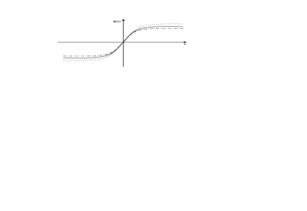
Figure 1: Plot of the deformed defects. The thick line shows the kink of the the $\phi^{4}$ model. The other lines show deformed kinks, the dashed-dotted line representing the $\sinh$-deformation, and the dotted line the ${\rm arcsinh}$-deformation.

We see that the $\sinh$-deformation diminishes the energy of the BPS solutions narrowing its distribution, and the ${\rm arcsinh}$-deformation operates in opposite direction, increasing the energy and spreading its distribution. These deformations are smooth deformations, which lead to potentials similar to the original potential. They map the interval $(-\infty,\infty)$ into itself, and their derivatives $f^{\prime}(\phi)$ have no divergence at any finite $\phi$. They teach us how to deform a given defect, changing its parameters in the two possible directions, decreasing or increasing the amplitude and width of the original defect. Since the amplitude and width of the defect are important to characterize the defect, the proposed deformations are of direct interest to applications involving kinks and walls in high energy physics and in condensed matter.

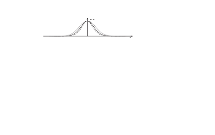
Figure 2: Plot of the energy density of the deformed defects. The thick line refers to the $\phi^{4}$ model. The other lines refer to the other cases, as explained in the previous figure.

The recent interest on tachyons t3 ; t4 ; t5 ; t6 ; t7 ; t8 ; t9 ; t10 has inspired us to extend the above procedure to nontopological or lump-like defects. We see that if $\phi(x)$ solves the equation of motion (1), then ${\widetilde{\phi}}(x)=f^{-1}(\phi)$ solves the equation of motion for the deformed model with potential ${\widetilde{V}}(\phi)=V[f(\phi)]/[f^{\prime}(\phi)]^{2}$. This is always true, for solutions that obey the first-order Eqs. (2), with energy density equally shared between gradient and potential portions.

A model which supports nontopological or lump-like solutions is

$$V_{l}(\phi)=\frac{1}{2}\phi^{2}(1-\phi^{2})$$ (27)

It has the solutions

$$\phi^{l}_{\pm}(x)=\pm{\rm sech}(x)$$ (28)

In quantum mechanics, the related problem has potential $U(x)=1-6\,{\rm sech^{2}(x)}$. This potential has the same form of the the modified Pösch-Teller potential [see the comments just above Eq. (19)]. However, it plots differently, shifting the values of $U(x)$ in a way such that the zero-mode is now identified with the upper bound state, making the lower bound state negative, signalling for tachyonic excitation.

We now consider deforming the lump-like solutions with $\sinh\phi$. We get

$${\widetilde{V}}_{l}(\phi)=\frac{1}{2}\tanh^{2}\phi(1-\sinh^{2}\phi)$$ (29)

The equation of motion for $\phi=\phi(x)$ is

$$\frac{d^{2}\phi}{dx^{2}}=\tanh\phi(1-\sinh^{2}\phi-2\tanh^{2}\phi)$$ (30)

It supports the deformed lump solutions

$${\widetilde{\phi}}^{l}_{\pm}=\pm{\rm arcsinh}[{\rm sech}(x)]$$ (31)

as we can verify straightforwardly. The deformation process may continue, and may also be done in the reverse direction, using ${\rm arcsinh}\phi$.

Similar investigations apply to other potentials. For instance, $V(\phi)=2\phi^{2}(1-\phi)$ supports the lump-like solution $\phi^{l}(x)={\rm sech}^{2}(x)$ – see Ref. t2 for further details on the $\phi^{3}$ model. We deform the lump-like solution with ${\rm arcsinh}\phi$. We get

$${\widetilde{V}}_{l}(\phi)=2(1+\phi^{2}){\rm arcsinh}^{2}\phi(1-{\rm arcsinh}\phi)$$ (32)

The deformed lump-like defect is

$${\widetilde{\phi}}_{l}(x)=\sinh[{\rm sech}^{2}(x)]$$ (33)

We can make the model supersymmetric introducing appropriate Majorana spinors. In this case, in general the Yukawa coupling is controlled by $Y(\phi)$, which has the form

$$Y(\phi)=\frac{d}{d\phi}\sqrt{2V(\phi)}$$ (34)

This leads to the usual coupling $Y(\phi)=W^{\prime\prime}(\phi)$ when the potential is given by $V(\phi)=(1/2)\,[W^{\prime}(\phi)]^{2}$, which is the form one uses to investigate kink-like structures. If one uses $f(\phi)$ to change the model from $V(\phi)=(1/2)\,[W^{\prime}(\phi)]^{2}$ to ${\widetilde{V}(\phi)}=(1/2)\,[W^{\prime}(f(\phi))/f^{\prime}(\phi)]^{2}$, the Yukawa coupling should also change from $Y(\phi)=W^{\prime\prime}(\phi)$ to

$${\widetilde{Y}}(\phi)=W^{\prime\prime}(f(\phi))-\frac{W^{\prime}(f(\phi))}{f^{\prime}(\phi)}\,\frac{f^{\,\prime\prime}(\phi)}{f^{\prime}(\phi)}$$ (35)

The importance of the deformation procedure that we have introduced enlarges if one recognizes that it admits deformations which lead to very different potentials, bearing no similarity to the original potential. Such deformations are different, and may lead to further interesting situations. For instance, we consider the function $f(\phi)=\tanh\phi$. It maps the interval $(-\infty,\infty)$ into the limited interval $(-1,1)$, and this allows introducing new effects, as we illustrate below.

We consider the potential

$$V(\phi)=\frac{1}{2}\,(1-\phi^{2})^{3}$$ (36)

This potential is new. It is unbounded below, containing a maximum at $\phi=0$ and two inflection points at $\pm 1$. In this case the modified potential becomes

$${\widetilde{V}}(\phi)=\frac{1}{2}\,{\rm sech}^{2}\phi$$ (37)

which is the vacuumless potential considered in cvi ; ba . In Ref. ba the vacuumless model was shown to support kink-like solutions of the BPS type. This result indicates that the model (36) may also support this kind of solutions. Indeed, it is astonishing to see that the potential (36) supports the kink-like defects

$$\phi(x)=\pm\frac{x}{\sqrt{1+x^{2}}}$$ (38)

which connect the two inflection points of the potential. These defects are stable, and they can be seen as deformations of the defects

$$\phi(x)=\pm{\rm arcsinh}(x)$$ (39)

which appear in the model defined by the potential of Eq. (37). As far as we know, this is the first example where kink-like defects connect two inflection points. In the recent Ref. jva one has found another model, somehow similar to the above one, but there the solution connects a local minimum to a inflection point.

The solutions (38) are stable, and the Schrödinger-like equation that appears in the investigation of stability is defined by the Hamiltonian

$$H=-\frac{d^{2}}{dx^{2}}+12\frac{x^{2}-1/4}{(x^{2}+1)^{2}}$$ (40)

The potential is a volcano-like potential, which supports the zero mode and no other bound state. The (normalized) wave function of the zero mode is $\eta_{0}(x)=2(2/3\pi)^{1/2}(x^{2}+1)^{-3/2}$. This should be contrasted with the zero mode of the vacuumless potential, which is given by ba : ${\widetilde{\eta}}_{0}(x)=(1/\pi)^{1/2}(x^{2}+1)^{-1/2}$. We notice that the two zero modes localize very differently in space.

The present work is of direct interest to investigations concerning systems described by two real scalar fields, as considered for instance in Refs. 2f ; bb . Also, it may be of some use in more complex situations, involving three or more scalar fields, in scenarios such as the one where we deal with the entrapment of planar network of defects bb01 , or with the presence of non-trivial solutions representing orbits that connect vacuum states in the three-dimensional configuration space blw .

The deformation scheme that we have presented may also work in other contexts, in particular in the case where one couples the scalar field to gravity in higher dimensions. We have found interesting investigations in Refs. g1 ; g2 ; g3 , and we are now considering the possibility of extending the deformation procedure to brane-world scenarios.

We would like to thank C.G. Almeida, F.A. Brito, and R. Menezes for discussions, and CAPES, CNPq, PROCAD and PRONEX for partial support.

References

- (1) A. Vilenkin and E.P.S. Shellard, Cosmic Strings and Other Topological Defects (Cambridge, Cambridge/UK, 1994).
- (2) R. Durrer, M. Kunz, and A. Melchiorri, Phys. Rep. 364, 1 (2002).
- (3) D. Walgraef, Spatio-Temporal Pattern Formation (Springer-Verlag, New York, 1997).
- (4) I. Cho and A. Vilenkin, Phys. Rev. D 59, 021701(R) (1999); D 59, 063510 (1999).
- (5) D. Bazeia, Phys. Rev. D 60, 067705 (1999).
- (6) R. Jackiw and C. Rebbi, Phys. Rev. D 13, 3398 (1976).
- (7) J. Goldstone and F. Wilczek, Phys. Rev. Lett. 47, 986 (1981).
- (8) W.P. Su, J.R. Schrieffer, and A.J. Heeger, Phys. Rev. Lett. 42, 1698 (1979).
- (9) M. Olshanii, Phys. Rev. Lett. 81, 938 (1998).
- (10) J. Ruostekoski, G.V. Dunne, and J. Javanainen, Phys. Rev. Lett. 88, 180401 (2002).
- (11) T.D. Lee, Phys. Rev. D 35, 3637 (1987).
- (12) J.A. Frieman, G.B. Gelmini, M. Gleiser, and E.W. Kolb, Phys. Rev. Lett. 60, 2101 (1988).
- (13) A.L. MacPherson and B.A. Campbell, Phys. Lett. B 347, 205 (1995).
- (14) J.R. Morris and D. Bazeia, Phys. Rev. D 54, 5217 (1996).
- (15) D. Coulson, Z. Lalak, and B. Ovrut, Phys. Rev. D 53, 4237 (1996).
- (16) E. Witten, Nucl. Phys. B 268, 253 (1986).
- (17) V.A. Kostelecký and S. Samuel, Phys. Lett. B 207, 169 (1988); Nucl. Phys. B 336, 263 (1990).
- (18) A. Sen, Int. J. Mod. Phys. A 14 4061 (1999); J. High Energy Phys. 12, 027 (1999).
- (19) J.A. Harvey and P. Kraus, J. High Energy Phys. 04, 012 (2000).
- (20) N. Moeller and W. Taylor, Nucl. Phys. B 583, 105 (2000).
- (21) R. de Mello Koch, A. Jevicki, M. Mihailescu and R. Tatar, Phys. Lett. B 482, 249 (2000).
- (22) N. Moeller, A. Sen, and B. Zwiebach, J. High Energy Phys. 08, 039 (2000).
- (23) B. Zwiebach, J. High Energy Phys. 09, 028 (2000).
- (24) J.A. Minahan and B. Zwiebach, J. High Energy Phys. 09, 029 (2000).
- (25) A. Fujii and H. Itoyama, Phys. Rev. Lett. 86, 5235 (2001).
- (26) M.K. Prasad and C.M. Sommerfield, Phys. Rev. Lett 35, 760 (1975).
- (27) E.B. Bogomol’nyi, Sov. J. Nucl. Phys. 24, 449 (1976).
- (28) D. Bazeia, J. Menezes, and M.M. Santos, Phys. Lett. B 521, 418 (2001); Nucl. Phys. B 636, 132 (2002).
- (29) L. Infeld and T.E. Hull, Rev. Mod. Phys. 23, 21 (1951).
- (30) F. Cooper, A. Khare, and U. Sukhatme, Phys. Rep. 251, 267 (1995).
- (31) D.P. Jatkar and R. Vathsan, J. High Energy Phys. 06, 039 (2001).
- (32) D. Bazeia, M.J. dos Santos, and R.F. Ribeiro, Phys. Lett. A 208, 84 (1995).
- (33) D. Bazeia and F.A. Brito, Phys. Rev. Lett. 84, 1094 (2000); Phys. Rev. D 61, 105019 (2000).
- (34) D. Bazeia and F.A. Brito, Phys. Rev. D 62, 101701(R) (2000); F.A. Brito and D. Bazeia, Phys. Rev. D 64, 065022 (2001).
- (35) D. Bazeia, L. Losano, and C. Wotzasek, Phys. Rev. D, to appear; hep-th/0206031.
- (36) M. Cvetic, S. Griffies, and S.-J. Rey, Nucl. Phys. B 381, 301 (1992).
- (37) K. Skenderis and P.K. Townsend, Phys. Lett. B 468, 46 (1999).
- (38) O. DeWolfe, D.Z. Freedman, S.S. Gubser and A. Karch, Phys. Rev. D 62, 046008 (2000).