The mass renormalization of nonperturbative light-front Hamiltonian theory: An illustration using truncated, Pauli–Villars-regulated Yukawa interactions

Abstract

We obtain analytic, nonperturbative, approximate solutions of Yukawa theory in the one-fermion sector using light-front quantization. The theory is regulated in the ultraviolet by the introduction of heavy Pauli–Villars scalar and fermion fields, each with negative norm. In order to obtain a directly soluble problem, fermion-pair creation and annihilation are neglected, and the number of bosonic constituents is limited to one of either type. We discuss some of the features of the wave function of the eigensolution, including its endpoint behavior and spin and orbital angular momentum content. The limit of infinite Pauli–Villars mass receives special scrutiny.

1 Introduction

It is remarkable that the first analysis of renormalization in quantum field theory was performed in the context of a nonperturbative problem – the QED calculation of the Lamb Shift in hydrogenic atoms by Bethe in 1948 [1]. In effect, one calculates the energy shift to order $\alpha$ and all orders in the atomic binding from the difference [2]:

$$\Delta E_{n}=<\overline{\psi_{n}}|\Sigma(Z\alpha)-\delta m|\psi_{n}>\,,$$ (1)

where $\Sigma(Z\alpha)$ is the order-$\alpha$ self energy of the electron evaluated in the background of the nuclear Coulomb potential $-Z\alpha\over r$, and $\delta m=\Sigma(Z=0)$ is the free-electron mass shift. The $-\delta m=m_{0}-m$ counterterm arises from the order-$\alpha$ contribution to the physical mass. As shown by Yennie and Erickson [2], the atomic energy shift $\Delta E_{n}$ can be evaluated in terms of the expectation values of gauge invariant operators which are functionals of the field strength $F_{\mu\nu}$ of the background field. The dominant term in the shift of the $nS$ levels is of order

$$\Delta E_{n}\sim{\alpha\over\pi}(Z\alpha)^{4}\ln{(Z\alpha)^{2}}m\,.$$ (2)

The logarithmic dependence indicates the inherently nonperturbative nature of the renormalization problem. The atomic-physics analysis of renormalization is appropriate to cases such as an infinitely heavy nucleus where the binding interaction is effectively static. In principle, one can take into account dynamical effects from retarded interactions and finite mass sources by using effective interaction methods [3].

Relativistic systems in quantum field theory can be analyzed by quantization on the light front [4] in a manner resembling nonrelativistic theory. The eigenstates of the invariant light-front Hamiltonian $H_{\rm LF}=P^{-}P^{+}-P^{2}_{\perp}$ satisfy the LF Heisenberg equation

$$H_{\rm LF}|\psi_{n}>=M^{2}_{n}|\psi_{n}>\,.$$ (3)

The eigenvalue problem can be rewritten in matrix form by introducing a free Fock basis. The matrix equation becomes discrete in momentum space by introducing periodic boundary conditions, as in the discrete light-cone quantization (DLCQ) method [5, 6]. The theory can be rendered ultraviolet finite by introducing Pauli–Villars (PV) ghost fields [7, 8, 9, 10, 11, 12, 13]. We have recently demonstrated the viability of this type of PV regularization by applying it to (3+1)-dimensional Yukawa theory of spin-half fermions and scalar bosons and have obtained nonperturbative DLCQ solutions of this theory in low particle number sectors [10]. We have also been able to solve such theories analytically in the limit of exact degeneracy of the negative and positive norm states [11]. Infrared divergences do not appear in neutral bound states such as color-singlet hadrons in QCD, since the gauge-particle interactions cancel at long wavelength.

The interaction terms in $H_{\rm LF}$ change particle number and contain the quantum effects associated with dressing the constituents analogous to $\Sigma(Z\alpha)$. The counterterms arising from the difference of the physical and bare mass of the massive constituents give a subtraction term [14] analogous to the subtraction term in Eq. (1), which is

$$\delta M^{2}_{n}=-\sum_{q}<\overline{\psi_{n}}|{\delta m_{q}^{2}\over x_{q}}|\psi_{n}>\,,$$ (4)

where ${1\over x_{q}}={P^{+}\over k^{+}_{q}}$ is evaluated within the sum over Fock states.

In practice, carrying out the above analysis is complicated in nonperturbative relativistic problems by the necessity that the Fock state has to be truncated. However, we do not perform sector-dependent renormalization [15], and instead retain the bare parameters of the original Lagrangian, the fermion mass and the coupling, as the only parameters to be adjusted. The shift in the fermion mass is the only counterterm. Contributions to the mass shift from instantaneous fermion interactions do not appear if one includes a negative-metric fermion as part of the Pauli–Villars regularization [11], since these instantaneous terms are mass independent.

In this paper we shall carry out the above nonperturbative mass renormalization program in the context of the LF Hamiltonian formulation of Yukawa theory. The interactions of a massive fermion and light scalar boson generate an effective fermion bound state, for which we are able to obtain approximate, but analytic, nonperturbative solutions. A set of negative-norm heavy scalar and fermion Pauli–Villars fields is used to regulate the ultraviolet divergences while preserving the chiral symmetry of the perturbative mass shift. In order to obtain a directly soluble problem, fermion-pair creation and annihilation are neglected, and the number of bosonic constituents is limited to one of either type. We shall discuss some of the features of the wave function of the eigensolution, including its endpoint behavior and spin and orbital angular momentum content. The dependence of the renormalized theory on the mass of the Pauli–Villars fields has some unexpected features which we discuss in detail.

In principle, the light-front wave functions of QCD can be computed directly by the diagonalization of the light-front Hamiltonian. The DLCQ method [5, 6] provides a discretization scheme which transforms the eigenvalue problem of QCD into the problem of diagonalizing very large sparse matrices. Although the Fock space is truncated, the DLCQ method retains the essential Lorentz symmetries of the theory including boost independence. DLCQ has also provided an important tool for analyzing string and higher dimension theories [16]. The DLCQ method has been successfully applied to QCD and other gauge theories in one space and one time dimensions [6]. There have also been applications of DLCQ to (3+1)-dimensional non-gauge theories [6].

Application to QCD₃₊₁ is computationally intensive [17], because of the large numbers of degrees of freedom; however, the solution of the bound-state eigenvalue problem corresponding to the hadronic spectrum would be a very important step. Given the projection of the eigensolutions on the light-front Fock basis, one can compute observables such as form factors and transition amplitudes [18, 19], the underlying features of deep inelastic scattering structure functions, the distribution amplitudes which control leading twist contributions to hard exclusive processes [20], and the skewed parton distributions which can be measured in deeply virtual Compton scattering [21, 22]. First-principle computations of exclusive decay amplitudes of heavy hadrons, such as the $D$ and $B$ mesons [23, 24], require knowledge of heavy and light hadron wave functions in order to extract the phases and other parameters of the electroweak theory. Light-front techniques can also be applied to traditional nuclear physics [25]. The light-front representation is boost-independent and provides the nonperturbative input and matrix elements required for such analyses.

An important feature of light-front Hamiltonian is the simplicity of spin and angular momentum projections: the sum rule for the angular momentum of the eigensolution $J^{z}=\sum^{n}_{i=1}S^{z}_{i}+\sum^{n-1}_{i=1}L^{z}_{i}$ holds Fock state by Fock state. Here the sum is over the spin projections $S_{z}$ of the constituents in the $n$-particle Fock state. There are only $n-1$ contributions to the internal orbital angular momentum. The spin projections also provide a convenient way to classify independent contributions to the wave functions. Our truncation to two partons limits $L^{z}_{i}$ to the values 0 and $\pm 1$.

In Sec. 2 we discuss the Yukawa Hamiltonian and its regularization and renormalization, as well as the Hamiltonian eigenvalue problem, which we solve, given the truncation to two particles. Since the methods we use are analytic, we are able to find two-parton solutions in the continuum theory without DLCQ or other discretization. We discuss the nature of the solutions in two limits, one in Sec. 3.1 where the PV masses are equal and another in Sec. 3.2 where the PV boson mass approaches infinity more slowly than the PV fermion mass. We are particularly interested in the chiral properties, the large transverse momentum fall-off, and the end-point behavior of the eigensolutions in the light-cone variables $x_{i}=k^{+}/P^{+}$ of the constituents. In Sec. 4 we argue that in calculations where the representation space is truncated, it is necessary to keep the values of the PV masses finite even in cases where it is computationally possible to take the limit of infinite PV masses. It is possible that some of the effects we see may be related to the triviality of Yukawa theory [26], but similar considerations probably apply to asymptotically free theories. Section 5 contains our conclusions.

Our calculations are somewhat similar to those of Bylev, Głazek, and Przeszowski [27], except that they did not use a covariant regulation procedure; it is the effect of the covariant regulator that will form the focus of our discussion here. Similar work in a purely scalar theory has been done by Bernard et al. [28]. For a more formal treatment of dressed constituents, see [29].

The notation that we use for light-cone coordinates is

$$x^{\pm}=x^{0}+x^{3}\,,\;\;\vec{x}_{\perp}=(x^{1},x^{2})\,.$$ (5)

The time coordinate is $x^{+}$, and the dot product of two four-vectors is

$$p\cdot x=\frac{1}{2}(p^{+}x^{-}+p^{-}x^{+})-\vec{p}_{\perp}\cdot\vec{x}_{\perp}\,.$$ (6)

The momentum component conjugate to $x^{-}$ is $p^{+}$, and the light-cone energy is $p^{-}$. Light-cone three-vectors are identified by underscores, such as

$$\underline{p}=(p^{+},\vec{p}_{\perp})\,.$$ (7)

For additional details, see Appendix A of Ref. [8] or the review [6].

2 Computational Framework

Taking the physical fermionic and bosonic fields to be $\psi_{1}$ and $\phi_{1}$, respectively, and the PV (negative-metric) fields to be $\psi_{2}$ and $\phi_{2}$, the Yukawa action becomes

$$S=\int d^{4}x \left[\frac{1}{2}(\partial_{\mu}\phi_{1})^{2}-\frac{1}{2}\mu_{1}^{2}\phi_{1}^{2}-\frac{1}{2}(\partial_{\mu}\phi_{2})^{2}+\frac{1}{2}\mu_{2}^{2}\phi_{2}^{2}\right.$$

$$+ \frac{i}{2}\left(\overline{\psi}_{1}\gamma^{\mu}\partial_{\mu}-(\partial_{\mu}\overline{\psi}_{1})\gamma^{\mu}\right)\psi_{1}-m_{1}\overline{\psi}_{1}\psi_{1}$$ (8)

$$\left.-\frac{i}{2}\left(\overline{\psi}_{2}\gamma^{\mu}\partial_{\mu}-(\partial_{\mu}\overline{\psi}_{2})\gamma^{\mu}\right)\psi_{2}+m_{2}\overline{\psi}_{2}\psi_{2}-g\phi\overline{\psi}\psi\right]\,,$$

where the scalar three-point interaction is expressed in terms of zero-norm fields

$$\psi\equiv(\psi_{1}+\psi_{2})\,,\quad\phi\equiv(\phi_{1}+\phi_{2})\,.$$ (9)

For simplicity, we will not consider a $\phi^{4}$ term; with pair creation removed, it will not be required.

If the bare mass of the fermion is zero, the bare action (the same as above but with the PV fields set equal to zero) possesses a discrete chiral symmetry – invariance under the transformations $\psi\rightarrow\gamma_{5}\psi$, $\phi\rightarrow-\phi$. One consequence of this symmetry is that the physical mass is also zero. The full action, including the PV fields breaks this symmetry explicitly. There are two possible versions of this breaking: if we require that the PV Fermi field is not transformed, the cross term in the interaction breaks the symmetry; if we require the PV Fermi field to transform in the same way as the physical field, the PV mass term breaks the chiral symmetry. Thus an interesting question, which we will examine below, is whether chiral symmetry will be restored in the limit of large PV masses where the unphysical states decouple. It will be a point of interest to see if the symmetry is restored, at least in the sense that the bare mass and the physical mass are proportional to each other.

The corresponding light-cone Hamiltonian, except for the addition of the PV fields, has been given by McCartor and Robertson [30]. Here we include the PV fields but neglect pair terms and any other terms which involve anti-fermions. The resulting Hamiltonian is

$$P^{-} = \sum_{i,s}\int d\underline{p}\frac{m_{i}^{2}+{\vec{p}}_{\perp}^{2}}{p^{+}}(-1)^{i+1}b_{i,s}^{\dagger}(\underline{p})b_{i,s}(\underline{p})$$

$$+\sum_{j}\int d\underline{q}\frac{\mu_{j}^{2}+{\vec{q}}_{\perp}^{2}}{q^{+}}(-1)^{j+1}a_{j}^{\dagger}(\underline{q})a_{j}(\underline{q})$$

$$+\sum_{i,j,k,s}\int d\underline{p}d\underline{q}\left\{\left[V_{-2s}^{*}(\underline{p},\underline{q})+V_{2s}(\underline{p}+\underline{q},\underline{q})\right]b_{j,s}^{\dagger}(\underline{p})a_{k}^{\dagger}(\underline{q})b_{i,-s}(\underline{p}+\underline{q})\right.$$

$$\left.+\left[U_{j}(\underline{p},\underline{q})+U_{i}(\underline{p}+\underline{q},\underline{q})\right]b_{j,s}^{\dagger}(\underline{p})a_{k}^{\dagger}(\underline{q})b_{i,s}(\underline{p}+\underline{q})+h.c.\right\}\,,$$

where

$$U_{j}(\underline{p},\underline{q})\equiv\frac{gm_{j}}{\sqrt{16\pi^{3}}}\frac{1}{p^{+}\sqrt{q^{+}}}\,,\;\;V_{2s}(\underline{p},\underline{q})\equiv\frac{g}{\sqrt{8\pi^{3}}}\frac{\vec{\epsilon}_{2s}^{\,*}\cdot\vec{p}_{\perp}}{p^{+}\sqrt{q^{+}}}\,,$$ (11)

$m_{1}$ is the mass of the bare fermion, $\mu\equiv\mu_{1}$ is the physical boson mass, $\mu_{2}$ and $m_{2}$ are the masses of the PV boson and fermion, respectively, and ${\vec{\epsilon}}_{2s}\equiv-\frac{1}{\sqrt{2}}(2s,i)$. The $V$ interaction introduces one unit of relative orbital angular momentum projection $L_{z}$ which is compensated by the change in fermion spin projection $S_{z}$ to conserve $J_{z}.$ [31]. The nonzero commutators are

$$\left[a_{i}(\underline{q}),a_{j}^{\dagger}(\underline{q}^{\prime})\right] = (-1)^{i}\delta_{ij}\delta(\underline{q}-\underline{q}^{\prime})\,,$$

$$\left\{b_{i,s}(\underline{p}),b_{j,s^{\prime}}^{\dagger}(\underline{p}^{\prime})\right\} = (-1)^{i}\delta_{ij}\delta_{s,s^{\prime}}\delta(\underline{p}-\underline{p}^{\prime})\,.$$ (12)

The Fock-state expansion for a spin-1/2 fermion eigenstate of the Hamiltonian is

$$\Phi_{\sigma} = \sum_{n_{1},n_{2},k_{1},k_{2}=0}^{\infty}\prod_{n=1}^{n_{\rm tot}}\int d\underline{p}_{n}\sum_{s_{n}}\prod_{k=1}^{k_{\rm tot}}\int d\underline{q}_{k}\delta(\underline{P}-\sum_{n}^{n_{\rm tot}}\underline{p}_{n}-\sum_{k}^{k_{\rm tot}}\underline{q}_{k})$$

$$\times\phi_{\sigma s_{n}}^{(n_{i},k_{j})}(\underline{p}_{n};\underline{q}_{k})\frac{1}{\sqrt{\prod_{i}n_{i}!\prod_{j}k_{j}!}}\prod_{n}^{n_{\rm tot}}b_{i_{n},s_{n}}^{\dagger}(\underline{p}_{n})\prod_{k}^{k_{\rm tot}}a_{j_{k}}^{\dagger}(\underline{q}_{k})|0\rangle\,,$$

where $n_{1}$ is the number of bare fermions, $n_{2}$ the number of PV fermions, $k_{1}$ the number of physical bosons, and $k_{2}$ the number of PV bosons. The total number of fermions is $n_{\rm tot}=n_{1}+n_{2}$, and the total number of bosons is $k_{\rm tot}=k_{1}+k_{2}$. The $n$-th constituent fermion is of type $i_{n}$, and the $k$-th boson is of type $j_{k}$. This Fock state expansion will be used to solve the eigenvalue problem $(P^{+}P^{-}{\vec{P}}^{2}_{\perp})\Phi_{\sigma}=M^{2}\Phi_{\sigma}$. The normalization of the eigenstate is

$$\Phi_{\sigma}^{\prime\dagger}\cdot\Phi_{\sigma}=\delta(\underline{P}^{\prime}-\underline{P})\,.$$ (14)

Our first approximation will be to truncate the expansion to two particles:

$$\Phi^{(2)}_{+}=\sum_{i}z_{i}b_{i+}^{\dagger}(\underline{P})|0\rangle+\sum_{ijs}\int d\underline{l}f_{ijs}(\underline{l})b_{i,s}^{\dagger}(\underline{P}-\underline{l})a_{j}^{\dagger}(\underline{l})|0\rangle$$ (15)

and reduce the eigenvalue problem by projecting onto Fock sectors. Without loss of generality, we consider only the $J_{z}=+1/2$ case. The resulting coupled equations determine the wave functions $f_{ij\pm}$ to be

$$f_{ij+}(\underline{l}) = \frac{P^{+}}{M^{2}-\frac{m_{i}^{2}+l_{\perp}^{2}}{1-l^{+}/P^{+}}-\frac{\mu_{j}^{2}+l_{\perp}^{2}}{l^{+}/P^{+}}}$$

$$\times\left[(\sum_{k}(-1)^{k+1}z_{k})U_{i}(\underline{P}-\underline{l},\underline{l})+\sum_{k}(-1)^{k+1}z_{k}U_{k}(\underline{P},\underline{l})\right]\,,$$

$$f_{ij-}(\underline{l}) = \frac{P^{+}}{M^{2}-\frac{m_{i}^{2}+l_{\perp}^{2}}{1-l^{+}/P^{+}}-\frac{\mu_{j}^{2}+l_{\perp}^{2}}{l^{+}/P^{+}}}(\sum_{k}(-1)^{k+1}z_{k})V_{+}^{*}(\underline{P}-\underline{l},\underline{l})\,,$$ (16)

corresponding respectively to Fock components where the fermion constituent is aligned or anti-aligned with the total spin $J_{z}.$ The nonperturbative physics is thus contained in the determination of $z_{i}$ and $M^{2}$. When the two-body wave functions $f$ are eliminated from the one-fermion projections, we obtain

$$(M^{2}-m_{i}^{2})z_{i} = g^{2}\mu_{1}^{2}(z_{1}-z_{2})J+g^{2}m_{i}(z_{1}m_{1}-z_{2}m_{2})I_{0}$$ (17)

$$+g^{2}\mu_{1}[(z_{1}-z_{2})m_{i}+z_{1}m_{1}-z_{2}m_{2}]I_{1}\,,$$

with

$$I_{n} = \int\frac{dydl_{\perp}^{2}}{16\pi^{2}}\sum_{jk}\frac{(-1)^{j+k}}{M^{2}-\frac{m_{j}^{2}+l_{\perp}^{2}}{1-y}-\frac{\mu_{k}^{2}+l_{\perp}^{2}}{y}}\frac{(m_{j}/\mu_{1})^{n}}{y(1-y)^{n}}\,,$$ (18)

$$J = \int\frac{dydl_{\perp}^{2}}{16\pi^{2}}\sum_{jk}\frac{(-1)^{j+k}}{M^{2}-\frac{m_{j}^{2}+l_{\perp}^{2}}{1-y}-\frac{\mu_{k}^{2}+l_{\perp}^{2}}{y}}\frac{(m_{j}^{2}+l_{\perp}^{2})/\mu_{1}^{2}}{y(1-y)^{2}}\,.$$ (19)

These integrals are not independent; a change of variable to $w=\frac{m_{j}^{2}+l_{\perp}^{2}}{1-y}+\frac{\mu_{k}^{2}+l_{\perp}^{2}}{y}$ and an interchange of integration order can be used to show that

$$J=\frac{M^{2}}{\mu_{1}^{2}}I_{0}\,.$$ (20)

We solve the $i=2$ case of Eq. (17) for $\zeta\equiv z_{2}/z_{1}$, to obtain

$$\zeta=\frac{g^{2}\mu_{1}^{2}J+g^{2}\mu_{1}(m_{1}+m_{2})I_{1}+g^{2}m_{1}m_{2}I_{0}}{M^{2}-m_{2}^{2}+g^{2}\mu_{1}^{2}J+2g^{2}\mu_{1}m_{2}I_{1}+g^{2}m_{2}^{2}I_{0}}\,.$$ (21)

From the remaining $i=1$ case we solve for $g^{2}$. This yields

$$g^{2}=-\frac{(M\mp m_{1})(M\mp m_{2})}{(m_{2}-m_{1})(\mu_{1}I_{1}\pm MI_{0})}\,.$$ (22)

There are two possible solutions for $g^{2}$ since the remaining equation is quadratic in $g^{2}$. Substitution into (21) and use of (20) reduces $\zeta$ to the remarkably simple form

$$\zeta=\frac{M\mp m_{1}}{M\mp m_{2}}\,,$$ (23)

independent of $I_{0}$ and $I_{1}$.

We pause here to remark that the wave function we have obtained in the nonperturbative calculation is very similar to the one which we would obtain using first-order perturbation theory to perturb about the state of one bare, physical fermion. The only differences are that in perturbation theory $z_{2}=0$ and $M=m_{1}$. From (23) we see that as $m_{2}\rightarrow\infty$, $\zeta=z_{2}/z_{1}$ will be small as long as $m_{1}<<m_{2}$. Since this last requirement is necessary if we are to expect to restore at least approximate unitarity in the limit of large PV masses, we will insist on it. The only significant difference between our nonperturbative calculation and first-order perturbation theory is that in perturbation theory $M=m_{1}$ while in the nonperturbative calculation $M$ is determined by (22). The form of the wave function in terms of the parameters is exactly the same in the perturbative and nonperturbative calculations; only the parameters are different.

In the presence of the negatively normed constituents, we define the “physical wave functions” as the coefficients of Fock states containing only positive-norm particles. This can be done without ambiguity by requiring that all Fock states be expressed in terms of the positive-norm creation operators $b_{1s}^{\dagger}$ and $a_{1}^{\dagger}$ and the zero-norm combinations $b_{s}^{\dagger}\equiv b_{1s}^{\dagger}+b_{2s}^{\dagger}$ and $a^{\dagger}\equiv a_{1}^{\dagger}+a_{2}^{\dagger}$. Because $b_{s}^{\dagger}$ is null, a fermion created by $b_{s}^{\dagger}$ is annihilated by the generalized electromagnetic current $(\overline{\psi}_{1}+\overline{\psi}_{2})\gamma^{\mu}(\psi_{1}+\psi_{2})$ appropriate to this PV-regulated theory; thus the null fermions do not contribute to current matrix elements and should not make a physical contribution to a state. By analogy, $a^{\dagger}$ is also deemed to create unphysical contributions. The procedure, then, is to express the wave function in terms the operators $b_{1s}^{\dagger}$, $b_{s}^{\dagger}$, $a_{1}^{\dagger}$ and $a^{\dagger}$ acting on the vacuum. Any term containing a $b_{s}^{\dagger}$ or an $a^{\dagger}$ is then discarded when constructing the physical state. This procedure is a non-orthogonal projection onto the physical subspace.

After application of this procedure to our case, the physical state with spin $J_{z}=+1/2$ in the two-particle truncation is

$$\Phi_{+{\rm phys}}^{(2)} = (z_{1}-z_{2})b_{1+}^{\dagger}(\underline{P})|0\rangle$$ (24)

$$+\sum_{i,j,s}\int d\underline{q}(-1)^{i+j}f_{ijs}(\underline{q})b_{1s}^{\dagger}(\underline{P}-\underline{q})a_{1}^{\dagger}(\underline{q})|0\rangle\,.$$

The normalization condition (14) fixes $z_{1}$. In addition to fixing the physical mass, one additional renormalization condition is needed. In previous papers [8, 9, 10] we have specified a value for the expectation value in the state

$$\langle:\!\!\phi^{2}(0)\!\!:\rangle\equiv\Phi_{\sigma}^{\dagger}\!:\!\!\phi^{2}(0)\!\!:\!\Phi_{\sigma}.$$ (25)

For some of the solutions given below this quantity diverges even after renormalization, so this is not a suitable condition. In the rest of the paper it is not necessary to specify the final renormalization condition. In place of specifying the final normalization condition, we will examine features of the solution. We will look for cases where the structure functions are finite and nonzero.

The normalization of $\Phi_{+{\rm phys}}^{(2)}$ and the definition of $\langle:\!\!\phi^{2}(0)\!\!:\rangle$ reduce to

$$1 = (z_{1}-z_{2})^{2}+\sum_{s}\int d\underline{l}\left|\sum_{ij}(-1)^{i+j}f_{ijs}(\underline{l})\right|^{2}\,,$$ (26)

$$\langle:\!\!\phi^{2}(0)\!\!:\rangle = \sum_{s}\int d\underline{l}\frac{2}{l^{+}/P^{+}}\left|\sum_{ij}(-1)^{i+j}f_{ijs}(\underline{l})\right|^{2}\,.$$ (27)

These relations can be written more explicitly in terms of the following integrals:

$$\tilde{I}_{0} = \int\frac{dy}{16\pi^{2}}i_{0}(y)\,,\;\;\tilde{I}^{\prime}_{0}=\int\frac{dy}{16\pi^{2}}\frac{2}{y}i_{0}(y)\,,$$ (28)

$$\tilde{I}_{1} = \int\frac{dy}{16\pi^{2}}i_{1}(y)\,,\;\;\tilde{I}^{\prime}_{1}=\int\frac{dy}{16\pi^{2}}\frac{2}{y}i_{1}(y)\,,$$

$$\tilde{J}_{0} = \int\frac{dy}{16\pi^{2}}j_{0}(y)\,,\;\;\tilde{J}^{\prime}_{0}=\int\frac{dy}{16\pi^{2}}\frac{2}{y}j_{0}(y)\,,$$

$$\tilde{J}_{1} = \int\frac{dy}{16\pi^{2}}j_{1}(y)\,,\;\;\tilde{J}^{\prime}_{1}=\int\frac{dy}{16\pi^{2}}\frac{2}{y}j_{1}(y)\,,$$

where

$$i_{0}(y) = \int dl_{\perp}^{2}\left(\sum_{jk}\frac{(-1)^{j+k}}{M^{2}-\frac{m_{j}^{2}+l_{\perp}^{2}}{1-y}-\frac{\mu_{k}^{2}+l_{\perp}^{2}}{y}}\right)^{2}\frac{\mu_{1}^{2}}{y}\,,$$ (29)

$$i_{1}(y) = \int dl_{\perp}^{2}\left(\sum_{jk}\frac{(-1)^{j+k}m_{j}}{M^{2}-\frac{m_{j}^{2}+l_{\perp}^{2}}{1-y}-\frac{\mu_{k}^{2}+l_{\perp}^{2}}{y}}\right)$$

$$\times\left(\sum_{jk}\frac{(-1)^{j+k}}{M^{2}-\frac{m_{j}^{2}+l_{\perp}^{2}}{1-y}-\frac{\mu_{k}^{2}+l_{\perp}^{2}}{y}}\right)\frac{\mu_{1}}{y(1-y)}\,,$$

$$j_{0}(y) = \int dl_{\perp}^{2}\left(\sum_{jk}\frac{(-1)^{j+k}m_{j}}{M^{2}-\frac{m_{j}^{2}+l_{\perp}^{2}}{1-y}-\frac{\mu_{k}^{2}+l_{\perp}^{2}}{y}}\right)^{2}\frac{1}{y(1-y)^{2}}\,,$$

$$j_{1}(y) = \int dl_{\perp}^{2}\left(\sum_{jk}\frac{(-1)^{j+k}}{M^{2}-\frac{m_{j}^{2}+l_{\perp}^{2}}{1-y}-\frac{\mu_{k}^{2}+l_{\perp}^{2}}{y}}\right)^{2}\frac{l_{\perp}^{2}}{y(1-y)^{2}}\,.$$

For the normalization and for $\langle:\!\!\phi^{2}(0)\!\!:\rangle$, we then obtain

$$\frac{1}{z_{1}^{2}} = (1-\zeta)^{2}[1+g^{2}(\tilde{J}_{0}+\tilde{J}_{1})]$$ (30)

$$+g^{2}\frac{(m_{1}-\zeta m_{2})^{2}}{\mu_{1}^{2}}\tilde{I}_{0}+2g^{2}(1-\zeta)\frac{m_{1}-\zeta m_{2}}{\mu_{1}}\tilde{I}_{1}\,,$$

$$\langle:\!\!\phi^{2}(0)\!\!:\rangle = g^{2}z_{1}^{2}\left\{(1-\zeta)^{2}[\tilde{J}^{\prime}_{0}+\tilde{J}^{\prime}_{1}]\right.$$ (31)

$$\left.+\frac{(m_{1}-\zeta m_{2})^{2}}{\mu_{1}^{2}}\tilde{I}^{\prime}_{0}+2(1-\zeta)\frac{m_{1}-\zeta m_{2}}{\mu_{1}}\tilde{I}^{\prime}_{1}\right\}\,.$$

The boson structure functions are given by

$$f_{Bs}(y)\equiv\int d^{2}l_{\perp}\left|\sum_{ij}(-1)^{i+j}f_{ijs}(yP^{+},{\vec{l}}_{\perp})\right|^{2}\,.$$ (32)

In terms of integrals already defined in (29) we obtain

$$f_{B+}(y) = \frac{g^{2}z_{1}^{2}}{16\pi^{2}}\left[(1-\zeta)^{2}j_{0}(y)+\frac{(m_{1}-\zeta m_{2})^{2}}{\mu_{1}^{2}}i_{0}(y)\right.$$ (33)

$$\left.+2(1-\zeta)\frac{(m_{1}-\zeta m_{2})}{\mu_{1}}i_{1}(y)\right]\,,$$

$$f_{B-}(y) = \frac{g^{2}z_{1}^{2}}{16\pi^{2}}(1-\zeta)^{2}j_{1}(y)\,.$$ (34)

As an alternative renormalization condition one could use the radius $R$ of the dressed-fermion state, as defined by the slope of the Dirac form factor $F_{1}$. These quantities are related by the standard expression $R=\sqrt{-6F^{\prime}_{1}(0)}$. The slope can be computed from the eigenfunction $\Phi_{+{\rm phys}}^{(2)}$ as

$$-\frac{R^{2}}{6}=F^{\prime}_{1}(0) = z_{1}^{2}\frac{g^{2}}{16\pi^{2}}\sum_{i^{\prime}j^{\prime}}(-1)^{i^{\prime}+j^{\prime}}\sum_{ij}(-1)^{i+j}\int_{0}^{1}\alpha(\alpha-1)d\alpha y^{3}dy$$

$$\times\left\{\left[(1-\zeta)^{2}m_{i}m_{i^{\prime}}+(m_{i}+m_{i^{\prime}})(1-\zeta)(m_{1}-\zeta m_{2})(1-y)\right.\right.$$

$$\left.\rule{108.405pt}{0.0pt}+(m_{1}-\zeta m_{2})^{2}(1-y)^{2}\right]/(D_{ij}^{i^{\prime}j^{\prime}})^{2}$$

$$\left.\rule{18.06749pt}{0.0pt}+2(1-\zeta)^{2}/D_{ij}^{i^{\prime}j^{\prime}}\right\}\,,$$

with $D_{ij}^{i^{\prime}j^{\prime}}\equiv\alpha(ym_{i^{\prime}}^{2}+(1-y)\mu_{j^{\prime}}^{2})+(1-\alpha)(ym_{i}^{2}+(1-y)\mu_{j}^{2})-y(1-y)M^{2}$. Similarly we can extract the axial coupling [32]

$$g_{A} = z_{1}^{2}(1-\zeta)^{2}+z_{1}^{2}\frac{g^{2}}{16\pi^{2}}\sum_{i^{\prime}j^{\prime}}(-1)^{i^{\prime}+j^{\prime}}\sum_{ij}(-1)^{i+j}\int_{0}^{1}d\alpha ydy$$

$$\times\left\{\left[(1-\zeta)^{2}m_{i}m_{i^{\prime}}+(m_{i}+m_{i^{\prime}})(1-\zeta)(m_{1}-\zeta m_{2})(1-y)\right.\right.$$

$$\left.\rule{144.54pt}{0.0pt}+(m_{1}-\zeta m_{2})^{2}(1-y)^{2}\right]/D_{ij}^{i^{\prime}j^{\prime}}$$

$$\left.\rule{18.06749pt}{0.0pt}+(1-\zeta)^{2}\log[2D_{ij}^{i^{\prime}j^{\prime}}]\right\}$$

and the anomalous magnetic moment $\kappa=F_{2}(0)$ of the dressed fermion

$$\kappa = 2Mz_{1}^{2}(1-\zeta)\frac{g^{2}}{16\pi^{2}}\sum_{i^{\prime}j^{\prime}}(-1)^{i^{\prime}+j^{\prime}}\sum_{ij}(-1)^{i+j}\int_{0}^{1}d\alpha y^{2}dy$$

$$\times\left[(1-\zeta)\left(\alpha m_{i^{\prime}}+(1-\alpha)m_{i}\right)+(m_{1}-\zeta m_{2})(1-y)\right]/D_{ij}^{i^{\prime}j^{\prime}}\,.$$

The result for the anomalous moment is confirmed by comparison with Eq. (51) of Ref. [31]. If the fermion $x$ in Ref. [31] is written as $1-y$ and the $M$ in the numerator is replaced by $m_{1}$, as per the discussion after Eq. (46), the two results agree, once we drop the sum over PV particles. Note that only the two-particle Fock state contributes since the anomalous moment requires a change in $L_{z}$ without a change in particle number.

As an example of how $R$ might be used as a renormalization condition, we compute $R$ and $g^{2}$ for a series of $m_{1}$ values, with $m_{2}=\mu_{2}=10\mu_{1}$ and $M$ fixed at $\mu_{1}$. We use the lower signs in Eqs. (22) and (23). The results are plotted in Fig. 1. The figures show that for a chosen value of $R$ and $M$ one can obtain values for the bare parameters $g$ and $m_{1}$, with the only ambiguity being between weak and strong coupling. The axial coupling is essentially constant over the given range, at a value very near unity. The anomalous moment is plotted in Fig. 2; here there is again the double-valued structure of the radius $R$. That the anomalous moment vanishes as $MR\to 0$ is consistent with the Drell–Hearn–Gerasimov sum rule, as discussed in [32].

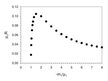
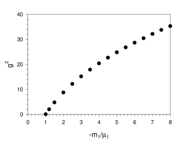
(a)	(b)

Figure 1: Plots of (a) the dressed-fermion radius $R$ and (b) the bare coupling squared $g^{2}$ as functions of the ratio of the bare fermion mass $m_{1}$ to the physical boson mass $\mu_{1}$. The PV masses are fixed at $m_{2}=\mu_{2}=10\mu_{1}$, and the dressed-fermion mass at $M=\mu_{1}$.

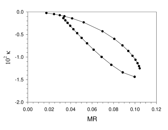
Figure 2: The anomalous moment $\kappa$ of the dressed fermion, multiplied by $10^{2}$, as a function of its radius $R$, scaled by its mass $M$. For this particular plot the dressed-fermion mass is set equal to the physical boson mass $\mu_{1}$, and the PV masses are fixed at $m_{2}=\mu_{2}=10\mu_{1}$. The solid lines are drawn to connect points on the same branch.

3 Limits for large Pauli–Villars Masses

3.1 Equal Pauli–Villars Masses

Although the nonperturbative problem has been reduced to a single nonlinear equation, and although all the integrals involved in that equation can be done in closed form, the resulting expression is very long and complex and, worse yet, is a function of many variables. To gain some control over the total space in which we will look for solutions, we will fix the ratio of the two PV masses. A natural choice seems to be $m_{2}=\mu_{2}$, especially if we choose $M$, the physical fermion mass, to be equal to $\mu_{1}$, the physical boson mass.

When the PV masses $m_{2}$ and $\mu_{2}$ are equal, and we make the assumption that $m_{1}<<m_{2}$, the integrals $I_{0}$ and $I_{1}$, multiplied by $16\pi^{2}$, reduce to $\log(m_{2}^{2}/m_{1}^{2})$ and $m_{2}/\mu_{1}$, respectively. We therefore find from (22) that

$$\frac{g^{2}}{16\pi^{2}}=-\frac{(M\mp m_{1})(M\mp m_{2})}{(m_{2}-m_{1})[m_{2}\mp M\log(m_{1}^{2}/m_{2}^{2})]}\,.$$ (38)

With this choice of the behavior of the PV masses, the integrals involved in the structure functions (33) and (34) have no singularities (in $m_{2}$) worse than logarithmic. From (38) we see that if $m_{1}$ stays finite or diverges more slowly than $m_{2}/\log m_{2}$ in the large-$m_{2}$ limit, $g$ will go to zero so fast that the structure functions must vanish, and we will have, in that sense, a trivial theory. A further examination of the particular choice $m_{1}\sim m_{2}/\log m_{2}$ shows that even in that case the structure functions go to zero as $m_{2}$ goes to infinity. The only choice for the behavior of $m_{1}$ as a function of $m_{2}$ which leads to finite, nonzero structure functions is $m_{1}\sim m_{2}$. We therefore define $r\equiv m_{1}/m_{2}$ and hold $r$ fixed as $\mu_{2}=m_{2}\rightarrow\infty$. The fractional amplitude $\zeta$ for the single-PV-fermion state, given in (23), becomes equal to $r$. The coupling is then driven to a fixed value

$$\frac{g^{2}}{16\pi^{2}}=\frac{-r}{1-r}\,.$$ (39)

Thus $m_{1}$ (and $r$) must be negative. The structure functions become

$$f_{B+}(y) \simeq -z_{1}^{2}r(1-r)\left[2+y+\frac{r^{2}y}{1+\left(r^{2}-1\right)\,y}\right.$$ (40)

$$-2\left(\frac{r\,\log(r^{2})}{r^{2}-1}-\frac{y\,\log(y)}{1-y}-\frac{r\ \,y\,\log(r^{2}\,y)}{r^{2}\,y-1}\right.$$

$$-\frac{r^{2}\,y\,}{1-y}\log(\frac{r^{2}\,y}{1-y+r^{2}\,y})+\frac{r\,\log(1-y+r^{2}\,y)}{r^{2}-1}$$

$$\left.\left.-\frac{ry}{1+\left(r^{2}-2\right)\,y}\log(\frac{1-y+r^{2}\,y}{y})\right)\right]\,,$$

$$f_{B-}(y) \simeq z_{1}^{2}r(1-r)(1-r^{2})\left(4y-\frac{\left(1+r^{2}\right)\,\,y\,\log(r^{2})}{r^{2}-1}+\frac{y(1+y)\log(y)}{1-y}\right.$$ (41)

$$+\frac{y\,\left(1+r^{2}\,y\right)\,\log(r^{2}\,y)}{r^{2}\,y-1}+\frac{y\,\left(1+\left(2\,r^{2}-1\right)\,y\right)}{1-y}\,\log(\frac{r^{2}\,y}{1-y+r^{2}\,y})$$

$$-\frac{\,\left(2+\left(r^{2}-1\right)\,y\right)\,\log(1-y+r^{2}\,y)}{r^{2}-1}$$

$$\left.+\frac{y\,\left(1+r^{2}\,y\right)}{1+\left(r^{2}-2\right)\,y}\log(\frac{1-y+r^{2}\,y}{y})\right)\,.$$

The nonorthogonal projection of the wave function ensures that these distributions are positive definite. The reciprocal of the factor $z_{1}^{2}$ is determined by the normalization condition (14) to be

$$\frac{1}{z_{1}^{2}} = (1-r)^{2}+\frac{1}{144}\frac{g^{2}}{16\pi^{2}}\left[4(27-108r+307r^{2})\right.-3\pi^{2}(6-24r+49r^{2})$$ (42)

$$\rule{108.405pt}{0.0pt}\left.-24(3-12r+20r^{2})\ln(r^{2})\right]$$

to second order in $r$. We thus have a one-parameter family of theories labeled by $r$. While the PV masses have been taken to infinity, they have not been made infinitely large compared to the bare fermion mass, which has been taken to minus infinity. The value of $g$ is finite in this limit. We probably should not, even naively, think that all the effects of the negatively normed states have been removed from the full solution. To control such effects, we should consider values of $r$ which are small in absolute value. Notice that $g$ is then restricted to small values.

The results of the exact solution are very different from perturbation theory. In first-order perturbation theory, $M$ is equal to $m_{1}$, and there is no nonlinear eigenvalue equation and thus no restriction of the value of $g$. Indeed, since the physical mass, $M$, is fixed and equal to $m_{1}$, we could not send $m_{1}$ to minus infinity as we did above. We also note that the discrete chiral symmetry is not restored in the large PV-mass limit. We cannot take $m_{1}$ to be zero (without obtaining a trivial theory). We can take the physical mass, $M$, to be zero, but that point does not occur at $m_{1}=0$.

Plots of the structure functions for $r=m_{1}/m_{2}=-0.01$ are given in Fig. 3. We should remark on the behavior of the structure functions at the end points. For very large values of the PV masses the functions are given essentially exactly by Eqs. (40) and (41) for all points except very close to $y=0$ in the case of $f_{B+}$. The exact structure functions are zero at $y=0$ for all values of the PV masses; yet (40) yields a nonzero value at that point. Thus the convergence to the limiting forms is nonuniform. For that reason, any quantity sensitive to the endpoint behavior, such as the expectation value of the parton light-cone kinetic energy, should be calculated for finite values of the PV masses and then taken to the infinite-mass limit.

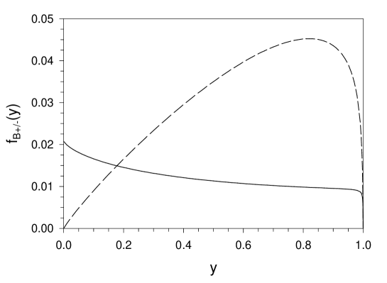
Figure 3: Structure functions $f_{B+}$ (solid) and $f_{B-}$ (dashed) for the equal-PV-mass case, with $r=m_{1}/m_{2}=-0.01$, from the forms given in Eqs. (40) and (41) of the text.

3.2 Unequal Pauli–Villars Masses

Having obtained the results discussed in the last subsection, one can ask whether there is any way to get results more like perturbation theory. As it turns out, there is: to do so we must take the limit of large PV masses in such a way that the PV fermion mass grows much faster than the PV boson mass.

If we take the mass $m_{2}$ to infinity, the integrals $I_{0}$ and $I_{1}$ reduce to

$$16\pi^{2}I_{0}\simeq-\log(\mu_{2}/\mu_{1})\,,\;\;16\pi^{2}I_{1}\simeq-2\frac{m_{1}}{\mu_{1}}\log(\mu_{2}/\mu_{1})\,.$$ (43)

The fractional amplitude $\zeta=(m_{1}\mp M)/m_{2}$ goes to zero. When we take $m_{2}\rightarrow\infty$ and then take $\mu_{2}$ large, the eigenvalue equation (22) becomes

$$\frac{g^{2}}{16\pi^{2}}=\frac{C}{\log(\mu_{2}/\mu_{1})}\,,$$ (44)

where

$$C=\left(\frac{m_{1}\mp M}{2m_{1}\pm M}\right)\,.$$ (45)

In this limit the structure functions reduce to

$$f_{B+}(y) = \frac{g^{2}z_{1}^{2}}{16\pi^{2}}\frac{(1\pm m_{1}/\mu_{1}-y)^{2}y\mu_{1}^{2}}{\mu_{1}^{2}(1-y)+m_{1}^{2}y-M^{2}y(1-y)}\,,$$ (46)

$$f_{B-}(y) = \frac{g^{2}z_{1}^{2}}{16\pi^{2}}y\left\{\log\left[\frac{(1-y)\mu_{2}^{2}}{\mu_{1}^{2}(1-y)+m_{1}^{2}y-M^{2}y(1-y)}\right]-2\right\}\,.$$ (47)

3.2.1 $m_{1}$ finite

Looking at these relations we see that if $g^{2}\sim 1/\log\mu_{2}$, $f_{B-}$ will be finite and nonzero while $f_{B+}$ will be zero in the limit of large PV mass. If $g^{2}$ remains finite, $f_{B+}$ will be finite and nonzero while $f_{B-}$ will diverge, which is untenable. There are two choices for the behavior of $m_{1}$ which will give us the desired behavior for $g^{2}$ and finite non-zero values for $f_{B-}(y)$. One way is to choose $m_{1}$ to be finite and choose its value and the signs in (45) such that the constant $C$ is any real number we wish. In that case, $f_{B-}$ is given by

$$f_{B-}(y)=2Cz_{1}^{2}y\,.$$ (48)

From (26) we find that

$$z_{1}^{2}=\frac{1}{1+C}\,.$$ (49)

Thus there is a finite probability that the state consists of a single physical fermion. The larger the value of $C$ the smaller is that probability and the larger is the probability that the state contains two particles. We note, as in the case of equal PV masses, that the discrete chiral symmetry is not restored in the sense that if we take either $M$ or $m_{1}$ equal to zero, the other is not specified and disappears entirely from the problem; the value of $C$ is fixed at either 1 or 1/2.

3.2.2 $m_{1}$ proportional to $M$

The other possibility for the behavior of $m_{1}$ is to choose $m_{1}\sim\pm\frac{M}{2}$ with the appropriate choice of sign in (45). For illustration we take the lower sign and parameterize

$$m_{1}=\frac{M}{2}+\frac{\mu_{1}}{2c\log(\mu_{2}/\mu_{1})}\,,$$ (50)

with $c$ a constant. With these choices the bare coupling constant goes to a finite value given by

$$\frac{g^{2}}{16\pi^{2}}=\frac{3Mc}{2}\,.$$ (51)

From this we see that $c$ should be positive. Notice that this choice is much more like perturbation theory: instead of $m_{1}=M$, as in first-order perturbation theory, we have (in the limit) $m_{1}=\frac{M}{2}$, and the coupling constant can be any finite number. In this case we find for large $\mu_{2}$ that $z_{1}^{2}$ is given by

$$z_{1}^{2}=\frac{2}{3Mc\log(\mu_{2}/\mu_{1})}\,.$$ (52)

There is zero probability that the system is in the state of one physical fermion, and the entire wave function is in the two-particle sector. Due to the behavior of $z_{1}$ we find again that, in the infinite-$\mu_{2}$ limit, $f_{B+}$ is zero while

$$f_{B-}(y)=2y\,.$$ (53)

The outcome for the discrete chiral symmetry in this case is not so clear. The fact that $m_{1}$ is proportional to $M$ (in the limit) suggests that it may be restored. On the other hand if $M$ is zero we would encounter undefined expressions in the above derivation. However, we can perform the entire calculation with $M$ set equal to zero from the start, and we find that if we take

$$m_{1}=\frac{\mu_{1}}{2c\log\frac{\mu_{2}}{\mu_{1}}}\,,$$ (54)

we obtain the structure function (53) and zero for $f_{B+}(y)$; this last result is in agreement with perturbation theory. So in that sense, the discrete chiral symmetry is restored in the large-PV-mass limit.

We should repeat the comment of the previous section regarding the behavior of the structure functions at the endpoints. For finite values of the PV masses, the structure functions vanish at $y=1$, but there is a nonuniform convergence. For very large values of the PV masses the structure function is closely proportional to $y$ for all values of $y$ except very near 1 where it falls precipitously to zero. In the limit of large PV masses the function converges to something proportional to $y$ for every point except $y=1$, where it is always zero. For that reason any quantity which is sensitive to the endpoint behavior (such as the kinetic energy of the fermion or $\langle:\!\!\phi^{2}(0)\!\!:\rangle$) should be calculated for finite values of the PV masses then the limit taken. If that exercise is performed for $\langle:\!\!\phi^{2}(0)\!\!:\rangle$, we find that this quantity does diverge.

4 On Not Taking the Limit

Up to now we have taken the limit of the PV masses going to infinity. Here we wish to further consider the comparison of our results with perturbation theory. We believe that this comparison suggests that we should not take that limit and furthermore indicates why we should not do so. These same considerations will suggest a way to decide how large we should take the PV masses.

Let us fix our attention on the choices made in Sec. 3.2.2 for taking the limit of large PV masses and fixing $m_{1}$, which gave results most like perturbation theory. The structure function $f_{B+}(y)$ was zero in that case. That does not happen in perturbation theory. Since our wave function is identical and even the parameters are almost the same (differing only in that $m_{1}=M/2$), how can we get something so different from perturbation theory? The reason we obtained zero for $f_{B+}$ is that the renormalization constant $z_{1}$ went to zero. If we look at the form of the function for finite PV mass, it is

$$f_{B-}(y)=\frac{g^{2}[\mbox{finite quantity}]}{1+g^{2}[\mbox{finite quantity}]+g^{2}[\mbox{finite quantity}]\log\mu_{2}}\,.$$ (55)

The denominator represents $z_{1}^{-2}$. Now in perturbation theory, since the numerator is already of order $g^{2}$, only the 1 in the denominator is used and the result is nonzero. Indeed, suppose we calculate some quantity which is finite to this order such as the anomalous magnetic moment. Again we would get a result of the form

$$\kappa=\frac{g^{2}[\mbox{finite quantity}]}{1+g^{2}[\mbox{finite quantity}]+g^{2}[\mbox{finite quantity}]\log\mu_{2}}\,.$$ (56)

If we use the methods of the previous section this quantity would again be zero. In perturbation theory that would not happen, again because the divergent term in the denominator would not be used with this numerator. Now the divergent term in the denominator would be used in a calculation to order $g^{4}$; but then there would be an order $g^{4}$ term in the numerator which would cancel the divergence of the term from the denominator and give a finite result. That is the way perturbation theory works. The point is this: we will have an accurate calculation only to the extent that the projection of the wave function onto the excluded Fock states is small. We know from past calculations [10] that this projection can be very small, sometimes even for the severe truncation we are considering here, but those results were for finite values of the PV masses. There will be divergences in the excluded Fock sectors, and we must anticipate that for sufficiently large values of the PV masses the projection of the wave function onto those sectors will not be small.

There are two types of error associated with having finite values of the PV masses: for PV masses too small we will have too much of the negative norm states in the system. We anticipate that such errors are approximately the larger of $\frac{m_{1}}{m_{P}}$ or $\frac{\mu_{1}}{m_{P}}$ where $m_{P}$ is the smallest PV mass. The other type of error is a large projection of the wave function onto the excluded Fock sectors. That error should be approximately

$$\frac{\langle\Phi_{+{\rm phys}}^{\prime}|\Phi_{+{\rm phys}}^{\prime}\rangle}{\langle\Phi_{+{\rm phys}}|\Phi_{+{\rm phys}}\rangle}$$ (57)

where $\Phi_{+{\rm phys}}^{\prime}$ is the projection of the wave function onto the lowest excluded Fock sector. The higher Fock wave function $\Phi_{+{\rm phys}}^{\prime}$ can be estimated using perturbation theory, perturbing about $\Phi_{+}$ with the projection of $P^{-}$ onto the excluded sectors being chosen as the perturbing operator. The first type of error, from negative-metric Fock states, decreases with increasing PV mass; the second type of error, the truncation error, will usually increase with increasing PV mass. Ideally we should choose the values of the PV masses to be the values where the two types of error are equal. The strategy for treating the nonperturbative system is to include more and more of the representation space in our calculation and to increase the value of the PV masses until the desired accuracy is achieved. How much of the space will be required will depend on the problem.

In later work we will attempt to make these comments quantitative by estimating the optimum values for the PV masses. Here we will illustrate the effects of not taking the limit, for the trajectory in which the PV masses are taken to large values as in Sec. 3.2.2. For infinite $m_{2}$ but finite $\mu_{2}$ ($=100\mu_{1}$), and with the eigenvalue equation solved by Eq. (50) and Eq. (51), the structure functions, $f_{B+}$ and $f_{B-}$ are plotted in Fig. 4. These are to be compared with the linear function (Eq. (53)) for $f_{B-}$, and zero for $f_{B+}$, which result if the limit of infinite PV masses is taken. The structure functions for the finite value of the mass $M$ resemble what one expects in a bound state.

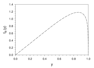
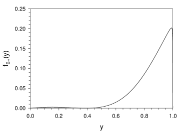
(a)	(b)

Figure 4: Structure functions (a) $f_{B-}$ and (b) $f_{B+}$ for the unequal-PV-mass case where $m_{2}\rightarrow\infty$, $\mu_{2}=100\mu_{1}$, and $M=\mu_{1}$. The bare fermion mass $m_{1}$ is specified by Eq. (50) of the text, and the coupling $g^{2}$ by Eq. (51), with $c=1$. Notice that the two plots have different vertical scales.

5 Discussion

In this paper we have studied the regulation of Yukawa theory by the use of Pauli–Villars fields in such a way that the interaction is written as a product of zero-norm fields. Paston and Franke have shown that this regulation procedure gives perturbative equivalence with Feynman methods [12]. The theory is covariant and presumably finite, and there are no gauge symmetries to protect. Therefore, if we could solve such a theory exactly and take the limit of the PV masses going to infinity, the result would be the best one could do to give a meaning to the theory. In this paper we have done our calculations in a severe truncation of the representation space. Such a truncation violates covariance, but if the contribution of excluded Fock sectors is sufficiently small, the consequence of the truncation is more a question of accuracy than of preserving symmetries: if we are close to the hypothetical solution mentioned above, it does not matter if this (small) error violates symmetries.

The reason we have used such a severe truncation is that it allows us to find solutions and take limits in closed form, and thus our interpretation of the results is not confounded by questions of inaccuracies introduced by numerical solutions. A significant feature of the calculations, which came as a surprise to us, is that the results depend strongly on the way in which the two PV masses are allowed to approach infinity. It is not true that any two different trajectories will give different results but rather that there are families of trajectories which give the same results. For instance, any trajectory on which the two PV masses are proportional to each other, with a fixed constant of proportionality, give the same result as taking the limit with the two masses set equal to each other. Similarly, any path on which $\mu_{2}$ is logarithmically small compared with $m_{2}$ will give the same result as taking the limit $m_{2}\rightarrow\infty$ first, then taking the limit $\mu_{2}\rightarrow\infty$. One possibility is that all these trajectories represent different phases of the theory. Another possibility is that the effect is an artifact of the truncation, and, if we include more and more of the representation space in the calculations, the results of the various ways of taking the limit will approach each other. Another possibility that we have considered is that some of the ways of taking the limit are wrong and that some principle which we have not yet discerned will determine the correct way to take the limit. We hope to report further studies on this question in the future.

In the calculations we have given special consideration to the discrete chiral symmetry that is formally present in the unregulated Lagrangian. Writing the interaction as a product of zero-norm fields breaks the chiral symmetry explicitly (unless the mass of the PV fermion is taken to be zero), and we have been careful to notice whether or not it is restored in the large-PV-mass limit, at least in the sense that the physical mass of the fermion is proportional to the bare mass. We find that for some ways of taking the limit the discrete chiral symmetry is restored and for some ways it is not. We do not know whether this consideration can provide a valid way of choosing one limiting procedure over another. This question is important because, not only is chiral symmetry of interest in itself, but the way it is broken by the regulation procedure is analogous to the way gauge symmetry is broken by writing the interactions of gauge theories as products of zero-norm fields.

We have argued that our results suggest that if calculations are done in a truncated representation space, it may not be correct to take the limit of the PV masses going all the way to infinity. It is easy to understand the reason why: if we are to have accurate calculations, most of the support of the wave functions in which we are interested must lie in the part of the space we retain. We know from past studies that the projection of the low-lying states onto the higher Fock sectors often falls off very rapidly in the light-cone representation, but those results were for finite values of the regulators. At infinite values of the regulators, the eigenvectors are not expected to exist at all, and we must expect that as the regulators are removed the projection of the wave functions onto any allowed sectors will become large. Thus it will be necessary to keep the PV masses finite when one truncates the representation space. If there are values of the PV masses sufficiently large to remove most of the bad effects of the negative-norm states on the eigenvectors in which we are interested, but small enough to make small the projection of these eigenvectors onto sectors we cannot manage to keep, then we can do a useful calculation; otherwise not. We are currently performing studies to try to make these remarks quantitative.

References

- [1] H.A. Bethe, Phys. Rev. 72 (1947), 339.
- [2] G.W. Erickson and D.R. Yennie, Ann. Phys. (N. Y.) 35 (1965), 271; (1965), 447; S.J. Brodsky and G. W. Erickson, Phys. Rev. 148 (1966), 26.
- [3] I. Blokland, A. Czarnecki, and K. Melnikov, Phys. Rev. D 65 (2002), 073015 [arXiv:hep-ph/0112267].
- [4] P.A.M. Dirac, Rev. Mod. Phys. 21 (1949), 392.
- [5] H.-C. Pauli and S.J. Brodsky, Phys. Rev. D 32 (1985), 1993; 32 (1985), 2001.
- [6] For reviews, see S.J. Brodsky and H.-C. Pauli, in “Recent Aspects of Quantum Fields” (H. Mitter and H. Gausterer, Eds.), Lecture Notes in Physics Vol. 396, p. 51, Springer-Verlag, Berlin, 1991; S.J. Brodsky, G. McCartor, H.-C. Pauli, and S.S. Pinsky, Part. World 3 (1993), 109; M. Burkardt, Adv. Nucl. Phys. 23 (1996), 1; S.J. Brodsky, H.-C. Pauli, and S.S. Pinsky, Phys. Rep. 301 (1997), 299 [arXiv:hep-ph/9705477].
- [7] W. Pauli and F. Villars, Rev. Mod. Phys. 21 (1949), 4334.
- [8] S.J. Brodsky, J.R. Hiller, and G. McCartor, Phys. Rev. D 58 (1998), 025005.
- [9] S.J. Brodsky, J.R. Hiller, and G. McCartor, Phys. Rev. D 60 (1999), 054506.
- [10] S.J. Brodsky, J.R. Hiller, and G. McCartor, Phys. Rev. D 64 (2001), 114023.
- [11] S.J. Brodsky, J.R. Hiller, and G. McCartor, Ann. Phys. 296 (2002), 406.
- [12] S.A. Paston and V.A. Franke, Theor. Math. Phys. 112 (1997), 1117 [Teor. Mat. Fiz. 112 (1997), 399] [arXiv:hep-th/9901110].
- [13] S.A. Paston, V.A. Franke, and E.V. Prokhvatilov, Theor. Math. Phys. 120 (1999), 1164 [Teor. Mat. Fiz. 120 (1999), 417] [arXiv:hep-th/0002062].
- [14] W.I. Weisberger, Phys. Rev. D 5 (1972), 2600.
- [15] R.J. Perry, A. Harindranath, and K.G. Wilson, Phys. Rev. Lett. 65 (1990), 2959.
- [16] T. Banks, W. Fischler, S.H. Shenker, and L. Susskind, Phys. Rev. D 55 (1997), 5112.
- [17] For an early attempt, see L.C.L. Hollenberg, K. Higashijima, R.C. Warner, and B.H.J. McKellar, Prog. Th. Phys. 87 (1992), 441.
- [18] S.J. Brodsky and S.D. Drell, Phys. Rev. D 22 (1980), 2236.
- [19] S.J. Brodsky and D.-S. Hwang, Nucl. Phys. B 543 (1999), 239 [arXiv:hep-ph/9806358].
- [20] S.J. Brodsky and G.P. Lepage, in “Perturbative Quantum Chromodynamics” (A.H. Mueller, Ed.), p. 93, World Scientific, Singapore, 1989.
- [21] S.J. Brodsky, M. Diehl, and D.-S. Hwang, Nucl. Phys. B 596 (2001), 99 [arXiv:hep-ph/0009254].
- [22] M. Diehl, T. Feldmann, R. Jakob, and P. Kroll, Nucl. Phys. B 596 (2001), 33 [Erratum-ibid. B 605 (2001), 647] [arXiv:hep-ph/0009255].
- [23] Y.Y. Keum, H.N. Li, and A.I. Sanda, Phys. Rev. D 63 (2001), 054008 [arXiv:hep-ph/0004173].
- [24] M. Beneke, G. Buchalla, M. Neubert and C.T. Sachrajda, Phys. Rev. Lett. 83 (1999), 1914 [arXiv:hep-ph/9905312].
- [25] G.A. Miller, Prog. Part. Nucl. Phys., 45 (2000), 83.
- [26] St.D. Głazek, A. Harindranath, S. Pinsky, J. Shigemitsu, and K. Wilson, Phys. Rev. D 47 (1993), 1599.
- [27] A.B. Bylev, S.D. Głazek, and J. Przeszowski, Phys. Rev. C 53 (1996), 3097.
- [28] D. Bernard, Th. Cousin, V.A. Karmanov, and J.-F. Mathiot, Phys. Rev. D 65 (2002), 025016.
- [29] St.D. Głazek and T. Maslowski, Phys. Rev. D 65 (2002), 065011; St.D. Głazek and M. Wieckowski, Phys. Rev. D 66 (2002), 016001.
- [30] G. McCartor and D.G. Robertson, Z. Phys. C 53 (1992), 679.
- [31] S.J. Brodsky, D.-S. Hwang, B.-Q. Ma, and I. Schmidt, Nucl. Phys. B 593 (2001), 311 [arXiv:hep-th/0003082].
- [32] F. Schlumpf and S.J. Brodsky, Phys. Lett. B 360 (1995), 1.