Phenomenological aspects of M–theory

Abstract

The Standard Model data suggests the realization of grand unification structures in nature, in particular that of $SO(10)$. A class of string vacua that preserve the $SO(10)$ embedding, are the three generation free fermion heterotic–string models, that are related to $Z_{2}\times Z_{2}$ orbifold compactification. Attempts to use the M–theory framework to explore further this class of models are discussed. Wilson line breaking of the $SO(10)$ GUT symmetry results in super–heavy meta–stable states, which produce several exotic dark matter and UHECR candidates, with differing phenomenological characteristics. Attempts to develop the tools to decipher the properties of these states in forthcoming UHECR experiments are discussed. It is proposed that quantum mechanics follows from an equivalence postulate, that may lay the foundations for the rigorous formulation of quantum gravity.

OUTP–02–34P

1 Introduction

Over the past few years important progress has been achieved in the basic understanding of string theory [1]. The picture that emerged, and which is depicted qualitatively in fig. 1, is that the different string theories in ten dimensions are perturbative limits of a single more fundamental theory. The vital question remains, how to relate these advances to observational data, as seen in terrestrial and astrophysical experiments. On the other hand, particle physics experiments over the past century cumulated in the Standard Particle Model. This model, and more importantly its experimental verification, represent the pinnacle of scientific achievement, and a source of elation for every participant in this magnificent endeavor.

What lesson should we extract then from the brilliant success of the Standard Model. An important aspect of the Standard Model is its multiplet structure, which is exhibited in fig. 2. The remarkable feature of the Standard Model is the embedding of its gauge and matter states into representations of Grand Unified Theories (GUTs) [2]. This astonishing fact seems almost a “triviality”. Namely, from a mathematical perspective the representations and associated group theory are rather mundane. The Standard Model multiplet structure is, however, what we observe experimentally, in multi–billion dollar collider experiments, and a priori there was no particular reason for this structure to emerge. The GUT embedding is most economical in the framework of $SO(10)$ [3], in which all the Standard Model states, including the right–handed neutrinos, which are desirable for neutrino masses and oscillations, in each generation, are embedded in a single 16 representation. Strikingly, each of the three generations fit into a spinorial 16 representation of $SO(10)$. If we regard the quantum numbers of the Standard Model states as experimental observables, as they were in the process of its experimental discovery, then, prior to unification, we count 54 free parameters. These include the quantum numbers of the three generations, each composed of six separate multiplets, under the Standard Model three group factors. The embedding in $SO(10)$ therefore reduces this number of free parameters from 54 to 3, which is the number of $SO(10)$ 16 representations needed to accommodate the Standard Model states. This to me looks like a true wonder of nature, and should serve as the guide in attempts to understand the fundamental origins of the Standard Model.

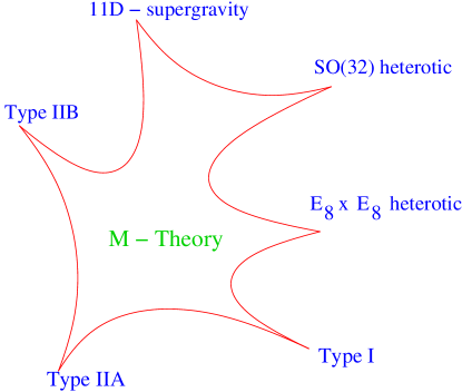
Figure 1: M–theory picture of string theory

While the Standard Model is confirmed, and its GUT generalizations are well motivated, by the experimental data, they leave many issues unresolved. The Higgs sector is unresolved experimentally and the associated electroweak symmetry breaking mechanism is still shrouded in mystery. Furthermore, the masses of the Higgs scalars cannot be protected against radiative corrections from the fundamental cut–off scale, a severe hierarchy problem. Finally the replication of the family flavors and the mass spectrum are not explained in the framework of Grand Unified Theories. It would therefore appear that these additional structures arise from physics above the GUT scale, where the gravitational interaction play a predominant role. String theory provides the unique framework to study how Planck scale physics determine these Standard Model structures.

1.1 High or low?

Indeed string theory, in its several perturbative incarnations, inspires much of the contemporary studies of physics beyond the Standard Model. From the experimental perspective the burning issue is the nature of the electroweak symmetry breaking mechanism and of the Higgs state. From a theoretical perspective the suppression of the electroweak scale, as compared to the fundamental GUT and gravitational scales, raises basic questions. To solve this puzzle two major school of thoughts have been developed. The first assumes the existence of new strongly interacting sector at the electroweak symmetry breaking scale. These include the old technicolor and composite Higgs theories, and their modern incarnations, in the form of large extra dimensions and warped compactifications. The second assumes that the Standard Model remains in the perturbative regime up to a scale which is of the order of the GUT and Planck scales. To stabilize the electroweak scale against radiative corrections from the larger scales one has to evoke the existence of a new symmetry, supersymmetry. The possibility of having a new strongly interacting sector at the TeV scale received a strong impetus in recent years due to the realization that the fundamental string unification scale can be lowered in the framework of M-theory [4].

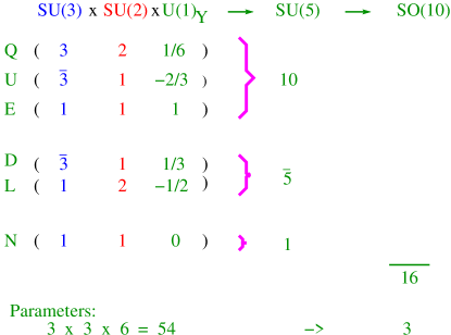
Figure 2: Standard Model multiplet structure

The problem that supersymmetry or a new strongly interacting sector at the TeV scale therefore address is the suppression of the scalar sector masses as compared to the fundamental unification scale, which is known as “The hierarchy problem”. The solutions invoked involve either the cancellation between fermionic and bosonic contributions to the Higgs boson masses (supersymmetry) or imposing that the cut–off scale is at the TeV scale (new strongly interacting sector; large extra dimensions; warped compactifications; etc). The natural question is whether these are mere alternatives, or whether one choice is preferred over the other. To contemplate this question we should examine the experimental data. The high scale unification paradigm is motivated by the Standard Model and Grand Unified Theories. In this context the hierarchy between the electroweak scale and the GUT or Planck scales arises due to the logarithmic running of the Standard Model parameters [5]. In the gauge sector of the Standard Model this logarithmic running has in fact been confirmed experimentally in the energy regime which is accessible to collider experiments. Namely by measuring the evolution of the Standard Model gauge parameters between the QCD scale and the  200 GeV scale probed at LEP, the logarithmic evolution agrees with observations. The assumption of the high scale unification is also in qualitative agreement with the data in the gauge and matter sectors of the Standard Model, as is exemplified by the resulting predictions for $\sin^{2}\theta_{W}(M_{Z})$ [5, 6] and for the mass ratio $M_{b}(M_{Z})/M_{\tau}(M_{Z})$ [7].

Thus supersymmetry maintains the logarithmic running in the gauge and matter sectors and restores it in the scalar sector. On the other hand a new strongly interacting sector (large extra dimensions; warped compactifications; etc) at the TeV scale annuls the logarithmic running in the gauge and matter sectors. We therefore note that, while supersymmetry has not yet been observed experimentally, logarithmic running, which is the origin of the hierarchy problem, has been observed experimentally in the gauge and matter sectors of the Standard Model. Therefore, theories which preserve this logarithmic running, which is the root for the hierarchical scales, are superior to those that do not.

2 Pheno–M–enology

The Standard Model and the low energy observed data support the existence of high scale unification and the big desert scenario. On the other hand, understanding many of the properties of the low energy data necessitates the incorporation of gravity into the unification program. Superstring theory provides a consistent perturbative approach to quantum gravity in which many of these issues can be studied. Due to the fundamental advances of recent years we know that the different string theories in ten dimensions are perturbative limits of a more fundamental theory, traditionally dubbed M–theory. This picture is qualitatively depicted in figure 1. In this context, the true fundamental theory of nature should have some nonperturbative realization. However, at present all we know about this more basic theory, are its perturbative string limits. Therefore, we should regard the perturbative string limits as providing tools to probe the properties of the fundamental nonperturbative vacuum in the different perturbative limits. As posited above the remarkable property of the Standard Model spectrum is the embedding of the chiral generations in the spinorial 16 representation of $SO(10)$. Thus, we may demand the existence of a viable perturbative string limit which preserve this embedding. The only perturbative string limit which enables the $SO(10)$ embedding of the Standard Model spectrum is the heterotic $E_{8}\times E_{8}$ string. The reason being that only this limit produces the spinorial 16 representation in the perturbative massless spectrum. Therefore, if we would like to preserve the $SO(10)$ embedding of the Standard Model spectrum, the M–theory limit which we should use is the perturbative heterotic string. In this respect it may well be that other perturbative string limits may provide more useful means to study other properties of the true nonperturbative vacuum, such as dilaton and moduli stabilization. This suggests the following approach to exploration of M–theory phenomenology. Namely, the true M-theory vacuum has some nonperturbative realization that at present we do not know how to formulate. This vacuum is at finite coupling and is located somewhere in the space of vacua enclosed by figure 1. The properties of the true vacuum can however be probed in the perturbative string limits. We may hypothesize that in any of these limits one still needs to compactify to four dimensions. Namely, that the true M–theory vacuum can still be formulated with four non–compact and all the other dimensions are compact. Then, suppose that in some of the limits we are able to identify a specific class of compactifications that possess appealing phenomenological properties. The new M–theory picture suggests that we can then explore the possible properties of the M–theory vacuum by studying compactifications of the other perturbative string limits on the same class of compactifications. This is the approach that we try to develop in the work described here.

The first task is therefore to construct string vacua that are as realistic as possible. Such a model of unification should of course satisfy a large number of constraints, a few of which are listed below,

$\underline{{\hbox{~{}~{}~{}~{}~{}~{}~{}~{}~{}~{}~{}~{}~{}~{}~{}~{}~{}~{}~{}~{}~{}~{}~{}~{}~{}~{}~{}~{}~{}~{}~{}~{}~{}~{}~{}~{}~{}}}}$

$1.$ Gauge group  $\longrightarrow$ $SU(3)\times SU(2)\times U(1)_{Y}$                $U(1)\in SO(10)$

$2.$ Contains three generations

$3.$ Proton stable         ($\tau_{\rm P}>10^{30+}$ years)

$4.$ N=1 supersymmetry        (or N=0)

$5.$ Contains Higgs doublets $\oplus$ potentially realistic Yukawa couplings

$6.$ Agreement with $\underline{\sin^{2}\theta_{W}}$ and $\underline{\alpha_{s}}$ at $M_{Z}$ (+ other observables).

$7.$ Light left–handed neutrinos

$~{}8.$ $SU(2)\times U(1)$ breaking

$~{}9.$ SUSY breaking

$10.$ No flavor changing neutral currents

$11.$ No strong CP violation

$12.$ Exist family mixing and weak CP violation

$13.$ +   …

$14.$ +                NO FREE EXOTICS

$\underline{{\hbox{~{}~{}~{}~{}~{}~{}~{}~{}~{}~{}~{}~{}~{}~{}~{}~{}~{}~{}~{}~{}~{}~{}~{}~{}~{}~{}~{}~{}~{}~{}~{}~{}~{}~{}~{}~{}~{}}}}$

The embedding of the Standard Model spectrum in $SO(10)$ representations implies that the weak hypercharge should have the canonical $SO(10)$ embedding. The $SO(10)$ symmetry need not be realized in an effective field theory but can be broken directly at the string level. In which case the Standard Model spectrum still arises from $SO(10)$ representations, but the $SO(10)$ non–Abelian states, beyond the Standard Model, are projected out by the GSO projections. However, if we take the Standard Model $SO(10)$ embedding as a necessary requirement this means that the weak hypercharge must have the standard $SO(10)$ embedding with $k_{Y}=5/3$.

The construction of realistic superstring vacua proceeds by studying compactification of the heterotic string from ten to four dimensions. Various methods can be used for this purpose which include geometric and algebraic tools, and each has its advantages and disadvantages. One class of models utilizes compactifications on Calabi–Yau 3–folds that give rise to an $E_{6}$ observable gauge symmetry, which is broken further by Wilson lines to $SU(3)^{3}$ [8]. This type of geometrical compactifications correspond at special points to conformal theories which have $(2,2)$ world–sheet supersymmetry. Similar compactifications which have only (2,0) world–sheet supersymmetry have also been studied and can lead to compactifications with $SO(10)$ and $SU(5)$ observable gauge groups [9]. The analysis of this type of compactification is complicated due to the fact that they do not correspond to free world–sheet theories. Therefore, it is difficult to calculate the parameters of the Standard Model in these constructions. On the other hand they provide a sophisticated mathematical window to the underlying geometry.

The next class of superstring vacua are the orbifold models [10]. Here one starts with a compactification of the heterotic string on a flat torus, using the Narain prescription [11], and utilizes free world–sheet bosons. The Narain lattice is moded out by some discrete symmetries which are the orbifold twisting. An important class of models of this type are the $Z_{3}$ orbifold models [12]. These give rise to three generation models with $SU(3)\times SU(2)\times U(1)^{n}$ gauge group. A deficiency of this class of models is that they do not give rise to the standard $SO(10)$ embedding of the Standard Model spectrum. Consequently, the normalization of $U(1)_{Y}$, relative to the non–Abelian currents, is typically larger than 5/3, the standard $SO(10)$ normalization. This results generically in disagreement with the observed low energy values for $\sin^{2}\theta_{W}(M_{Z})$ and $\alpha_{s}(M_{Z})$. A thorough analysis of $Z_{3}$ orbifold model was performed recently by Giedt [13], who also demonstrated the existence of models in this class which admit the $SU(5)$ embedding of the Standard Model gauge group.

The final class of perturbative string compactifications consist of those that are constructed from world–sheet conformal field theories. The simplest of those correspond to the free fermionic formulation in which all the degrees of freedom needed to cancel the conformal anomaly are represented in terms of free fermions propagating on the string world–sheet [14]. This in turn correspond to compactifications at fixed radii, and non–trivial background metric and antisymmetric tensor fields. More complicated world–sheet conformal field theories can also be formulated and, in general, correspond to compactifications at fixed radii [15].

It is important to emphasize that we expect that the different formulations of string compactifications are related. This in particular means that by utilizing these various tools one is not probing different physics. Thus, the different constructions can be used to study different aspects of specific classes of string compactifications. Naturally, we expect that some issues are better examined by using a particular formulation, whereas for others another may prove advantageous.

The concrete class of string models that form the basis of our studies here are those that are constructed in the free fermionic formulation. In the next section I briefly review the models. It is vital to note that this class of string compactifications correspond to $Z_{2}\times Z_{2}$ orbifold twisting of the Narain lattice which is realized at the free fermionic point in moduli space, and augmented with additional Wilson lines. The correspondence of a subset of these models with the $Z_{2}\times Z_{2}$ orbifold compactification [16] is exploited in attempts to elevate the study of these models to the nonperturbative regime. This construction gives rise naturally to two of the key propertied of the observed Standard Model particle spectrum. Specifically, it naturally produces three chiral generations with the canonical $SO(10)$ embedding. Roughly speaking the origin of three generations arises in the $Z_{2}\times Z_{2}$ orbifold based constructions, due to the fact that we are dividing a six dimensional compactified manifold into factors of two. Specifically, we have that the $Z_{2}\times Z_{2}$ orbifold twisting of a six dimensional compactified lattice produces exactly three twisted sectors. In the realistic free fermionic models one generation is obtained from each of the three twisted sectors. Thus, heuristically speaking the origin of three generations in these models is traced to

$${6\over 2}=3.$$

The natural question in the context of M–theory is how this naive understanding extend to the nonperturbative domain. However, the mere fact that we trace here the origin of three generations to the basic structure of the underlying compactification suggests that it is independent of the perturbative expansion. The second crucial property of the realistic free fermionic models is that they preserve the canonical $SO(10)$ embedding of the Standard Model spectrum. Consequently, the free fermionic construction produces a large class of three generation models, with differing phenomenological details.

3 Free fermionic models

I discuss here briefly the structure of the free fermionic models that forms the basis of our explorations. Phenomenological aspects of these models have been reviewed in the past in this conference series [17]. I recap the structure of the models which is most relevant for the specific pheno–M–enological aspects of M–theory that are of interest here.

A model in the free fermionic formulation [14] is defined by a set of boundary condition basis vectors, and one–loop GSO phases, which are constrained by the string consistency requirements, and completely determine the vacuum structure of the models. The physical spectrum is obtained by applying the generalized GSO projections. The Yukawa couplings and higher order nonrenormalizable terms in the superpotential are obtained by calculating correlators between vertex operators [18]. The realistic free fermionic models produce an “anomalous” $U(1)$ symmetry, which generates a Fayet–Iliopoulos D–term [19], and breaks supersymmetry at the Planck scale. Supersymmetry is restored by assigning non vanishing VEVs to a set of Standard Model singlets in the massless string spectrum along flat F and D directions. In this process nonrenormalizable terms, $\langle{V_{1}^{f}V_{2}^{f}V_{3}^{b}\cdot\cdot\cdot\cdot V_{N}^{b}\rangle},$ become renormalizable operators, $V_{1}^{f}V_{2}^{f}V_{3}^{b}{{\langle V_{4}^{b}\cdots V_{N}^{b}\rangle}/{M^{N-3}}}$ in the effective low energy field theory.

The first five basis vectors of the realistic free fermionic models consist of the NAHE set [20]. The gauge group after the NAHE set is $SO(10)\times E_{8}\times SO(6)^{3}$ with $N=1$ space–time supersymmetry, and 48 spinorial $16$ of $SO(10)$, sixteen from each sector $b_{1}$, $b_{2}$ and $b_{3}$. The three sectors $b_{1}$, $b_{2}$ and $b_{3}$ are the three twisted sectors of the corresponding $Z_{2}\times Z_{2}$ orbifold compactification. The $Z_{2}\times Z_{2}$ orbifold is special precisely because of the existence of three twisted sectors, with a permutation symmetry with respect to the horizontal $SO(6)^{3}$ charges.

The NAHE set is common to a large class of three generation free fermionic models. The construction proceeds by adding to the NAHE set three additional boundary condition basis vectors which break $SO(10)$ to one of its subgroups: $SU(5)\times U(1)$ [21], $SO(6)\times SO(4)$ [22], $SU(3)\times SU(2)\times U(1)^{2}$ [23, 24, 25, 26], or $SU(3)\times U(1)\times SO(4)$ [27]. At the same time the number of generations is reduced to three, one from each of the sectors $b_{1}$, $b_{2}$ and $b_{3}$. The various three generation models differ in their detailed phenomenological properties. However, many of their characteristics can be traced back to the underlying NAHE set structure. One such important property to note is the fact that as the generations are obtained from the three twisted sectors $b_{1}$, $b_{2}$ and $b_{3}$, they automatically possess the Standard $SO(10)$ embedding. Consequently the weak hypercharge, which arises as the usual combination $U(1)_{Y}=1/2U(1)_{B-L}+U(1)_{T_{3_{R}}}$, has the standard $SO(10)$ embedding.

The massless spectrum of the realistic free fermionic models then generically contains three generations from the three twisted sectors $b_{1}$, $b_{2}$ and $b_{3}$, which are charged under the horizontal symmetries. The Higgs spectrum consists of three pairs of electroweak doublets from the Neveu–Schwarz sector plus possibly additional one or two pairs from a combination of the two basis vectors which extend the NAHE set. Additionally the models contain a number of $SO(10)$ singlets which are charged under the horizontal symmetries and a number of exotic states.

Exotic states arise from the basis vectors which extend the NAHE set and break the $SO(10)$ symmetry [28]. Consequently, they carry either fractional $U(1)_{Y}$ or $U(1)_{Z^{\prime}}$ charge. Such states are generic in superstring models and impose severe constraints on their validity. In some cases the exotic fractionally charged states cannot decouple from the massless spectrum, and their presence invalidates otherwise viable models [29, 30]. In the NAHE based models the fractionally charged states always appear in vector–like representations. Therefore, in general mass terms are generated from renormalizable or nonrenormalizable terms in the superpotential. However, the mass terms which arise from non–renormalizable terms will in general be suppressed, in which case the fractionally charged states may have intermediate scale masses. The analysis of ref. [26] demonstrated the existence of free fermionic models with solely the MSSM spectrum in the low energy effective field theory of the Standard Model charged matter. In general, unlike the “standard” spectrum, the “exotic” spectrum is highly model dependent.

4 Phenomenological studies of free fermionic string models

I summarize here some of the highlights of the phenomenological studies of the free fermionic models. This demonstrates that the free fermionic string models indeed provide the arena for exploring many the questions relevant for the phenomenology of the Standard Model and Unification. The lesson that should be extracted is that the underlying structure of these models, generated by the NAHE set, produces the right features for obtaining realistic phenomenology. It provides further evidence for the assertion that the true string vacuum is connected to the $Z_{2}\times Z_{2}$ orbifold in the vicinity of the free fermionic point in the Narain moduli space. Many of the important issues relating to the phenomenology of the Standard Model and supersymmetric unification have been discussed in the past in several prototype free fermionic heterotic string models. These studies have been reviewed in the past and I refer to the original literature and additional review references [31, 17]. These include among others: top quark mass prediction [25], several years prior to the actual observation by the CDF/D0 collaborations [32]; generations mass hierarchy [33]; CKM mixing [34]; superstring see–saw mechanism [35]; Gauge coupling unification [36]; Proton stability [37]; and supersymmetry breaking and squark degeneracy [38]. Additionally, it was demonstrated in ref. [26] that at low energies the model of ref. [23], which may be viewed as a prototype example of a realistic free fermionic model, produces in the observable sector solely the MSSM charged spectrum. Therefore, the model of ref. [23], supplemented with the flat F and D solutions of ref. [26], provides the first examples in the literature of a string model with solely the MSSM charged spectrum below the string scale. Thus, for the first time it provides an example of a long–sought Minimal Superstring Standard Model! We have therefore identified a neighborhood in string moduli space which is potentially relevant for low energy phenomenology. While we can suggest arguments, based on target–space duality considerations why this neighborhood may be selected, we cannot credibly argue that similar results cannot be obtained in other regions of the string moduli space. Nevertheless, the results summarized here provide the justification for further explorations of the free fermionic models. Furthermore, they provide motivation to study these models in the nonperturbative context of M–theory. In this context the basis for our studies is the connection of the free fermionic models with the $Z_{2}\times Z_{2}$ orbifold, to which I turn in section 6.

I would like to emphasize that it is not suggested that any of the realistic free fermionic models is the true vacuum of our world. Indeed such a claim would be folly. Each of the phenomenological free fermionic models has its shortcomings, that if time and space would have allowed could have been detailed. While in principle the phenomenology of each of these models may be improved by further detailed analysis of supersymmetric flat directions, it is not necessarily the most interesting avenue for exploration. The aim of the studies outlined above is to demonstrate that all of the major issues, pertaining to the phenomenology of the Standard Model and unification, can in principle be addressed in the framework of the free fermionic models, rather than to find the explicit solution that accommodates all of these requirements simultaneously. The reason being that even within this space of solutions there is till a vast number of possibilities, and we lack the guide to select the most promising one. What is being proposed is that these phenomenological studies suggest that the true string vacuum may share some of the gross structure of the free fermionic models. Namely, it will possess the structure of the $Z_{2}\times Z_{2}$ orbifold in the vicinity of the free fermionic point in the Narain moduli space. This perspective provides the motivation for the continued interest in the detailed study of this gross structure, and specifically in the framework of M–theory, as discussed below.

5 Toward string predictions

Before turning to the recent M–theory related studies, I briefly discuss possible signatures of the string models, beyond the Standard Model. Following the demonstration of phenomenological viability of a class of string compactifications, it is sensible to seek possible experimental signals that may provide evidence for specific models in particular, and for string theory in general. This is in essence a secondary task as the first duty is to reproduce the observed physics of the Standard Model. With these priorities in mind there are several possible exotic signatures that have been discussed in the past. These include the possibility of extra $U(1)$’s [39]; specific supersymmetric spectrum scenarios [40]; R–parity violation [41]; and exotic matter [28]. R–parity violation at an observable rate is an intriguing but somewhat remote possibility. The problem is that in string models if R–parity is violated at the same time one expects to generate fast proton decay. The model of ref. [42] provides an example how R–parity violation can arise in superstring theory. This string model gives rise to custodial symmetries which allow lepton number violation while forbidding baryon number violation.

The second possibility is that of additional $Z^{\prime}$ gauge bosons in energy regimes that may be accessible to future colliders [39, 43]. This possibility is motivated by the need to suppress proton decay, while at the same time insuring that the masses of the left–handed neutrinos are adequately suppressed [44, 43]. In the context of string constructions a conflict may arise due to the fact that one typically utilizes VEVs that break the $B-L$ symmetry spontaneously. Such VEVs are used, for example, in the flipped $SU(5)$ to break the $SU(5)$ GUT symmetry. In other string models such VEVs typically must be used to generate a seesaw mechanism. The need to use $B-L$ breaking VEVs for this purpose follows from the absence of the $SO(10)$ 126 representation in the perturbative massless string spectrum [45]. On the other hand the $B-L$ breaking VEVs may induce rapid proton decay from dimension four operators. However, dimension four and five proton decay mediating operators may be adequately suppressed if the dangerous terms are forbidden by an additional $U(1)$ symmetry. In this case the effective magnitude of the proton decay mediating operators is determined by the symmetry breaking scale of the extra $U(1)$, and may be adequately suppressed provided that $\Lambda_{Z^{\prime}}$ is sufficiently small. String models produce $U(1)$ symmetries with the required properties that are external to the GUT symmetries. Typically, they will be family dependent and are therefore also constrained by the flavor data. However, such a $U(1)$ symmetry can remain unbroken down to $\sim 30$TeV and may have observable consequences in future colliders and/or flavor experiments.

The last possibility that I discuss here is that of exotic matter, which arises in superstring models because of the breaking of the non–Abelian symmetries by Wilson–lines [46, 28]. It is therefore a unique signature of superstring unification, which does not arise in field theory GUTs. While the existence of such states imposes severe constraints on otherwise valid string models [29], provided that the exotic states are either confined or sufficiently heavy, they can give rise to exotic signatures. For example, they can produce heavy dark matter candidates, possibly with observable consequences [47, 48, 49]. In section 8 I will elaborate on the exotic matter in the string models and possible observable consequences.

6 $Z_{2}\times Z_{2}$ orbifold correspondence

The key property of the fermionic models that is exploited in trying to elevate the analysis of these models to the nonperturbative domain of M–theory is the correspondence with the $Z_{2}\times Z_{2}$ orbifold compactification. As discussed in section 3 the construction of the realistic free fermionic models can be divided into two parts. The first part consist of the NAHE–set basis vectors and the second consists of the additional boundary conditions, $\{\alpha,\beta,\gamma\}$ that correspond to Wilson lines in the orbifold language. The correspondence of the NAHE-based free fermionic models with the orbifold construction is illustrated by extending the NAHE set, $\{1,S,b_{1},b_{2},b_{3}\}$, by one additional boundary condition basis vector [16],

$$\xi_{1}=(0,\cdots,0|{\underbrace{1,\cdots,1}_{{\bar{\psi}^{1,\cdots,5}},{\bar{\eta}^{1,2,3}}}},0,\cdots,0)~{}.$$ (1)

With a suitable choice of the GSO projection coefficients the model possesses an ${\rm SO}(4)^{3}\times{\rm E}_{6}\times{\rm U}(1)^{2}\times{\rm E}_{8}$ gauge group and $N=1$ space-time supersymmetry. The matter fields include 24 generations in the 27 representation of ${\rm E}_{6}$, eight from each of the sectors $b_{1}\oplus b_{1}+\xi_{1}$, $b_{2}\oplus b_{2}+\xi_{1}$ and $b_{3}\oplus b_{3}+\xi_{1}$. Three additional 27 and $\overline{27}$ pairs are obtained from the Neveu-Schwarz $\oplus~{}\xi_{1}$ sector.

To construct the model in the orbifold formulation one starts with the compactification on a torus with nontrivial background fields [11]. The subset of basis vectors,

$$\{1,S,\xi_{1},\xi_{2}\},$$ (2)

generates a toroidally-compactified model with $N=4$ space-time supersymmetry and ${\rm SO}(12)\times{\rm E}_{8}\times{\rm E}_{8}$ gauge group. The same model is obtained in the geometric (bosonic) language by tuning the background fields to the values corresponding to the SO(12) lattice. The metric of the six-dimensional compactified manifold is then the Cartan matrix of SO(12), while the antisymmetric tensor is given by

$$B_{ij}=\cases{G_{ij}&;\ $i>j$,\cr 0&;\ $i=j$,\cr-G_{ij}&;\ $i<j$.\cr}$$ (3)

When all the radii of the six-dimensional compactified manifold are fixed at $R_{I}=\sqrt{2}$, it is seen that the left- and right-moving momenta $P^{I}_{R,L}=[m_{i}-{1\over 2}(B_{ij}{\pm}G_{ij})n_{j}]{e_{i}^{I}}^{*}$reproduce the massless root vectors in the lattice of SO(12). Here $e^{i}=\{e_{i}^{I}\}$ are six linearly-independent vielbeins normalized so that $(e_{i})^{2}=2$. The ${e_{i}^{I}}^{*}$ are dual to the $e_{i}$, with $e_{i}^{*}\cdot e_{j}=\delta_{ij}$.

Adding the two basis vectors $b_{1}$ and $b_{2}$ to the set (2) corresponds to the ${Z}_{2}\times{Z}_{2}$ orbifold model with standard embedding. Starting from the Narain model with ${\rm SO}(12)\times{\rm E}_{8}\times{\rm E}_{8}$ symmetry [11], and applying the ${Z}_{2}\times{Z}_{2}$ twist on the internal coordinates, reproduces the spectrum of the free-fermion model with the six-dimensional basis set $\{1,S,\xi_{1},\xi_{2},b_{1},b_{2}\}$. The Euler characteristic of this model is 48 with $h_{11}=27$ and $h_{21}=3$. I denote the manifold corresponding to this model as $X_{2}$.

It is noted that the effect of the additional basis vector $\xi_{1}$ of eq. (1), is to separate the gauge degrees of freedom, spanned by the world-sheet fermions $\{{\bar{\psi}}^{1,\cdots,5},{\bar{\eta}}^{1},{\bar{\eta}}^{2},{\bar{\eta}}^{3},{\bar{\phi}}^{1,\cdots,8}\}$, from the internal compactified degrees of freedom $\{y,\omega|{\bar{y}},{\bar{\omega}}\}^{1,\cdots,6}$. In the realistic free fermionic models this is achieved by the vector $2\gamma$ [16], with

$$2\gamma=(0,\cdots,0|{\underbrace{1,\cdots,1}_{{\bar{\psi}^{1,\cdots,5}},{\bar{\eta}^{1,2,3}}{\bar{\phi}}^{1,\cdots,4}}},0,\cdots,0)~{},$$ (4)

which breaks the ${\rm E}_{8}\times{\rm E}_{8}$ symmetry to ${\rm SO}(16)\times{\rm SO}(16)$. The ${Z}_{2}\times{Z}_{2}$ twist breaks the gauge symmetry to ${\rm SO}(4)^{3}\times{\rm SO}(10)\times{\rm U}(1)^{3}\times{\rm SO}(16)$. The orbifold still yields a model with 24 generations, eight from each twisted sector, but now the generations are in the chiral 16 representation of SO(10), rather than in the 27 of ${\rm E}_{6}$. The same model can be realized with the set $\{1,S,\xi_{1},\xi_{2},b_{1},b_{2}\}$, by projecting out the $16\oplus{\overline{16}}$ from the $\xi_{1}$-sector taking

$$c{\xi_{1}\choose\xi_{2}}\rightarrow-c{\xi_{1}\choose\xi_{2}}.$$ (5)

This choice also projects out the massless vector bosons in the 128 of SO(16) in the hidden-sector ${\rm E}_{8}$ gauge group, thereby breaking the ${\rm E}_{6}\times{\rm E}_{8}$ symmetry to ${\rm SO}(10)\times{\rm U}(1)\times{\rm SO}(16)$. The freedom in (5) corresponds to a discrete torsion in the toroidal orbifold model. At the level of the $N=4$ Narain model generated by the set (2), we can define two models, ${Z}_{+}$ and ${Z}_{-}$, depending on the sign of the discrete torsion in eq. (5). The first, say ${Z}_{+}$, produces the ${\rm E}_{8}\times{\rm E}_{8}$ model, whereas the second, say ${Z}_{-}$, produces the ${\rm SO}(16)\times{\rm SO}(16)$ model. The ${Z}_{2}\times{Z}_{2}$ twist acts identically in the two models, and their physical characteristics differ only due to the discrete torsion eq. (5).

This analysis confirms that the ${Z}_{2}\times{Z}_{2}$ orbifold on the SO(12) Narain lattice is indeed at the core of the realistic free fermionic models. However, it differs from the ${Z}_{2}\times{Z}_{2}$ orbifold on $T_{2}^{1}\times T_{2}^{2}\times T_{2}^{3}$, which gives $(h_{11},h_{21})=(51,3)$. I will denote the manifold of this model as $X_{1}$. In [50] it was shown that the two models may be connected by adding a freely acting twist or shift. Let us first start with the compactified $T^{1}_{2}\times T^{2}_{2}\times T^{3}_{2}$ torus parameterized by three complex coordinates $z_{1}$, $z_{2}$ and $z_{3}$, with the identification

$$z_{i}=z_{i}+1\,,\qquad z_{i}=z_{i}+\tau_{i}\,,$$ (6)

where $\tau$ is the complex parameter of each $T_{2}$ torus. With the identification $z_{i}\rightarrow-z_{i}$, a single torus has four fixed points at

$$z_{i}=\{0,{\textstyle{1\over 2}},{\textstyle{1\over 2}}\,\tau,{\textstyle{1\over 2}}(1+\tau)\}.$$ (7)

With the two ${Z}_{2}$ twists

$$\alpha:(z_{1},z_{2},z_{3})\rightarrow(-z_{1},-z_{2},~{}~{}z_{3})\,,$$ (8)

$$\beta:(z_{1},z_{2},z_{3})\rightarrow(~{}~{}z_{1},-z_{2},-z_{3})\,,$$ (9)

there are three twisted sectors in this model, $\alpha$, $\beta$ and $\alpha\beta=\alpha\cdot\beta$, each producing 16 fixed tori, for a total of 48. Adding to the model generated by the ${Z}_{2}\times{Z}_{2}$ twist in (9), the additional shift

$$\gamma:(z_{1},z_{2},z_{3})\rightarrow(z_{1}+{\textstyle{1\over 2}},z_{2}+{\textstyle{1\over 2}},z_{3}+{\textstyle{1\over 2}})$$ (10)

produces again fixed tori from the three twisted sectors $\alpha$, $\beta$ and $\alpha\beta$. The product of the $\gamma$ shift in (10) with any of the twisted sectors does not produce any additional fixed tori. Therefore, this shift acts freely. Under the action of the $\gamma$-shift, the fixed tori from each twisted sector are paired. Therefore, $\gamma$ reduces the total number of fixed tori from the twisted sectors by a factor of ${2}$, yielding $(h_{11},h_{21})=(27,3)$. This model therefore reproduces the data of the ${Z}_{2}\times{Z}_{2}$ orbifold at the free-fermion point in the Narain moduli space.

A comment is in order here in regard to the matching of the model that include the shift and the model on the $SO(12)$ lattice. We noted above that the freely acting shift (10), added to the ${Z}_{2}\times{Z}_{2}$ orbifold at a generic point of $T_{2}^{1}\times T_{2}^{2}\times T_{2}^{3}$, reproduces the data of the ${Z}_{2}\times{Z}_{2}$ orbifold acting on the SO(12) lattice. This observation does not prove, however, that the vacuum which includes the shift is identical to the free fermionic model. While the massless spectrum of the two models may coincide their massive excitations, in general, may differ. The matching of the massive spectra is examined by constructing the partition function of the ${Z}_{2}\times{Z}_{2}$ orbifold of an SO(12) lattice, and subsequently that of the model at a generic point including the shift. In effect since the action of the ${Z}_{2}\times{Z}_{2}$ orbifold in the two cases is identical the problem reduces to proving the existence of a freely acting shift that reproduces the partition function of the SO(12) lattice at the free fermionic point. Then since the action of the shift and the orbifold projections are commuting it follows that the two ${Z}_{2}\times{Z}_{2}$ orbifolds are identical.

On the compact coordinates there are actually three inequivalent ways in which the shifts can act. In the more familiar case, they simply translate a generic point by half the length of the circle. As usual, the presence of windings in string theory allows shifts on the T-dual circle, or even asymmetric ones, that act both on the circle and on its dual. More concretely, for a circle of length $2\pi R$, one can have the following possibilities [51]:

$$A_{1}\;: X_{\rm L,R}\to X_{\rm L,R}+{\textstyle{1\over 2}}\pi R\,,$$

$$A_{2}\;: X_{\rm L,R}\to X_{\rm L,R}+{\textstyle{1\over 2}}\left(\pi R\pm{\pi\alpha^{\prime}\over R}\right)\,,$$

$$A_{3}\;: X_{\rm L,R}\to X_{\rm L,R}\pm{\textstyle{1\over 2}}{\pi\alpha^{\prime}\over R}\,.$$ (11)

There is an important difference between these choices: while $A_{1}$ and $A_{3}$ can act consistently on any number of coordinates, level-matching requires instead that $A_{2}$ acts on (mod) four real coordinates. By studying the respective partition function one finds [52] that the shift that reproduces the $SO(12)$ lattice at the free fermionic point in the moduli space is generated by the ${Z}_{2}\times{Z}_{2}$ shifts

$$g\;: (A_{2},A_{2},0)\,,$$

$$h\;: (0,A_{2},A_{2})\,,$$ (12)

where each $A_{2}$ acts on a complex coordinate. It is then shown that the partition function of the SO(12) lattice is reproduced. at the self-dual radius, $R_{i}=\sqrt{\alpha^{\prime}}$. On the other hand, the shifts given in Eq. (10), and similarly the analogous freely acting shift given by $(A_{3},A_{3},A_{3})$, do not reproduce the partition function of the $SO(12)$ lattice. Therefore, the shift in eq. (10) does reproduce the same massless spectrum and symmetries of the ${Z}_{2}\times{Z}_{2}$ at the free fermionic point, but the partition functions of the two models differ! Thus, the free fermionic ${Z}_{2}\times{Z}_{2}$ is realized for a specific form of the freely acting shift given in eq. (12). However, as we saw, all the models that are obtained from $X_{1}$ by a freely acting ${Z}_{2}$-shift have $(h_{11},h_{21})=(27,3)$ and hence are connected by continuous extrapolations. The study of these shifts in themselves may therefore also yield additional information on the vacuum structure of these models and is worthy of exploration.

Despite its innocuous appearance the connection between $X_{1}$ and $X_{2}$ by a freely acting shift has profound consequences. First we must realize that any string construction can only offer a limited glimpse on the structure of string vacua that possess some realistic characteristics. Thus, the free fermionic formulation gave rise to three generation models that were utilized to study issues like Cabbibo mixing and neutrino masses. On the other hand the free fermionic formulation is perhaps not the best suited to study issues that are of a more geometrical character. We can regard the free fermionic formulation as heavy duty machinery enabling detailed analysis near a single point in moduli space, but obscuring its gross structures. The geometrical approach on the other hand provides such a gross overview, but is perhaps less adequate in extracting detailed properties. However, as the precise point where the detailed properties should be calculated is not yet known, one should regard the phenomenological success of the free fermionic models as merely highlighting a particular class of compactified spaces. These manifolds then possess the overall structure that may accommodate the detailed Standard Model properties. The precise localization of where these properties should be calculated, will require further understanding of the string dynamics. But, if the assertion that the class of relevant manifolds has been singled out proves to be correct, this is already an enormous advance and simplification.

From the Standard Model data we may hypothesize that any realistic string vacuum should possess at least two ingredients. First, it should contain three chiral generations, and second, it should admit their SO(10) embedding. This SO(10) embedding is not realized in the low energy effective field theory limit of the string models, but is broken directly at the string level. The main phenomenological implication of this embedding is that the weak-hypercharge has the canonical GUT embedding.

It has long been argued that the ${Z}_{2}\times{Z}_{2}$ orbifold naturally gives rise to three chiral generations. The reason being that it contains three twisted sectors and each of these sectors produces one chiral generation. The existence of exactly three twisted sectors arises, essentially, because we are modding out a three dimensional complex manifold, or a six dimensional real manifold, by ${Z}_{2}$ projections, which preserve the holomorphic three form. Thus, metaphorically speaking, the reason being that six divided by two equals three.

However, this argument would hold for any ${Z}_{2}\times{Z}_{2}$ orbifold of a six dimensional compactified space, and in particular it holds for the $X_{1}$ manifold. Therefore, we can envision that this manifold can produce, in principle, models with SO(10) gauge symmetry, and three chiral generations from the three twisted sectors. However, the caveat is that this manifold is simply connected and hence the SO(10) symmetry cannot be broken by the Hosotani-Wilson symmetry breaking mechanism [53]. The consequence of adding the freely acting shift (10) is that the new manifold $X_{2}$, while still admitting three twisted sectors is not simply connected and hence allows the breaking of the SO(10) symmetry to one of its subgroups.

Thus, we can regard the utility of the free fermionic machinery as singling out a specific class of compactified manifolds. In this context the freely acting shift has the crucial function of connecting between the simply connected covering manifold to the non-simply connected manifold. Precisely such a construction has been utilized in [54] to construct non-perturbative vacua of heterotic M-theory. In the next section I discuss these phenomenological aspects of M–theory.

7 M–theory explorations

The profound new understanding of string theory that emerged over the past few years means that we can use any of the perturbative string limits, as well as eleven dimensional supergravity to probe the properties of the fundamental M–theory vacuum. The pivotal property that this vacuum should preserve is the $SO(10)$ embedding of the Standard Model spectrum. Additionally, the underlying compactification should allow for the breaking of the $SO(10)$ gauge symmetry. In string theory the prevalent method to break the $SO(10)$ gauge group is by utilizing Wilson line symmetry breaking.

These two properties are not found in generic string vacua, but are afforded by the realistic free fermionic models. The free fermionic models are, however, constructed in the perturbative heterotic string limit and it is therefore natural to examine which of their structures is preserved in the nonperturbative limit. The nonperturbative limit of the heterotic string is conjectured to be given by the heterotic M–theory limit, or by compactifications of the Hořava–Witten model [55] on Calabi–Yau threefolds. Hořava–Witten theory consists of compactifications of eleven dimensional supergravity on $S_{1}/Z_{2}$. The orbifold fixed points support ten dimensional supergravity, with a $E_{8}$ gauge supermultiplet on each fixed ten dimensional plane, and the bulk space consists of pure supergravity. To construct viable vacua of Hořava–Witten theory one needs to compactify further to four dimensions on a Calabi–Yau manifold.

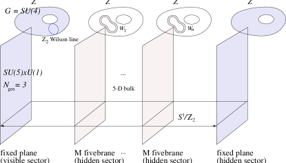
Figure 3: Compactifications of Horava–Witten theory to four dimensions

Heterotic M–theory compactifications to four dimensions have been studied by Donagi et al. [54], on manifolds that do not admit Wilson line breaking and yield $SU(5)$, $SO(10)$ or $E_{6}$ grand unified gauge groups, as well as construction of $SU(5)$ grand unified models that can be broken to the Standard Model gauge group by Wilson line breaking. In ref. [56] we extended the work of Donagi et alto the case of $SO(10)$ models that allow Wilson line breaking. This entails the modification of the gauge bundle analysis of ref. [54] from $G=SU(2n+1)$ to $G=SU(2n)$ in the decomposition of $E_{8}\supset G\times H$, where $H=SO(10)$ in our case. The structure of the manifolds constructed by Donagi et alcorrespond to manifolds with fundamental group ${\bf Z}_{2}$, which is necessary for Wilson line breaking. In this case the M–theory vacuum allows for $SO(10)$ breaking by a single Wilson–line.

The construction of Donagi et al. is very similar in spirit to the connection between the $X_{1}$ and $X_{2}$ manifolds discussed in section 6, but utilizes a different mathematical language. As the construction is quite technical, I will not review it here in detail, but merely give a qualitative overview with few additional insights from the free fermionic analogy. The qualitative picture is depicted in figure 3. In this picture The 11–dimensional spacetime $M_{11}$ of M–theory is taken to be

$$M_{11}=M_{4}\times{S^{1}\over{\bf Z}_{2}}\times Z,$$ (13)

where $M_{4}$ is 4–dimensional Minkowski spacetime, the compact eleventh dimension $S^{1}$ is moded out by the action of ${\bf Z}_{2}$, and $Z$ is a Calabi–Yau (complex) 3–fold. There is a semistable holomorphic vector bundle $V_{i}$, $i=1,2$ over the 3–fold $Z$ on the orbifold fixed plane at each of the two fixed points of the ${\bf Z}_{2}$–action on $S^{1}$. The structure group $G_{i}$ of $V_{i}$ is a subgroup of the observable $E_{8}$. The new feature of heterotic M–theory as compared to the perturbative heterotic string is the existence of fivebranes in the vacuum, which wrap holomorphic 2–cycles within $Z$ and are parallel to the orbifold fixed planes. The fivebranes are represented by a 4-form cohomology class $[W]$. The Calabi–Yau 3–fold $Z$, the gauge bundles $V_{i}$ and the fivebranes are subject to the cohomological constraint on $Z$

$$c_{2}(V_{1})+c_{2}(V_{2})+[W]=c_{2}(TZ),$$ (14)

where $c_{2}(V_{i})$ is the second Chern class of the $i$–th gauge bundle and $c_{2}(TZ)$ is the second Chern class of the holomorphic tangent bundle to $Z$. Equation (14) above is the anomaly–cancellation condition.

The construction of Donagi et alis based on generalization of earlier work of Friedman, Morgan and Witten (FMW) [57]. One starts in this construction with a Calabi–Yau manifold that admits an elliptic fibration (denoted $X\equiv X_{1}$). The Calabi–Yau threefold then consist of a base, which is a two dimensional complex manifold and a fiber, which is an elliptic curve. Friedman, Morgan and Witten derived expressions for the Chern classes of the gauge and tangent bundles in terms of the parameters of the base and the fiber and by utilizing the spectral cover construction. The derivation of FMW applies to fibrations which admit a global section. Solutions of different M–theory vacua, that contain three chiral generations with a GUT gauge group are then given by writing the effective cohomology classes of the five branes, $[W]$. These effective classes are compatible with wrappings of the five branes on real 2-cycles of the Calabi–Yau threefolds.

The existence of a global section in the fibration of $X$ implies that it is simply connected and hence does not admit GUT Wilson line breaking. Donagi et alproceed to mod out the $X$–manifold by a freely acting $Z_{2}$ involution, $\tau_{X}$, analogous to (10), yielding a manifold which is not simply connected (denoted $Z\equiv X_{2}$). The key difference between the $X$ and $Z$ manifolds is that the former admits a global section, whereas the later does not. The $Z$–manifold admits two sections that are interchanged by the freely acting involution. This implies that the $Z$ manifold admits a torus fibration but not an elliptic fibration. Additionally, while $\tau_{X}$ is freely acting on the Calabi–Yau threefold, it is not freely acting on the base. Hence, one must blow–up the singular curves on the base. The involution is guaranteed to be freely acting by requiring that the intersection of the fixed points of the involution with the zeroes of the discriminant of the Weierstrass form of the fiber is empty. Finally, the expressions for the Chern classes of the gauge and tangent bundles and the effective classes of the five branes are adopted to the case of the toroidally fibered Calabi–Yau manifold and solutions are found for three generation vacua.

In ref. [56] we presented such explicit solutions with $SO(10)$ symmetry broken by a Wilson line to $SU(5)\times U(1)$, which is the flipped $SU(5)$ symmetry breaking pattern [58]. We should note that the construction utilizes a single shift and yields $\Pi_{1}=Z_{2}$. This implies that we can break the $SO(10)$ symmetry by a single Wilson line. Hence, the $SO(10)$ can be broken by a single step to $SU(5)\times U(1)$ or $SO(6)\times SO(4)$ but not directly to the Standard Model gauge group. Similarly, in the the models built by Donagi et ala single Wilson line can be utilized to break the $SU(5)$ symmetry. However, there a single breaking step suffices to break $SU(5)$ directly to the Standard Model gauge group. While the construction of toroidally fibered manifolds that permit two–step Wilson line breaking is still underway, we may gain some insight from the free fermionic analogs as to what might perhaps be needed. Namely, in the free fermionic realization of these compactifications we know explicitly that two, or three, Wilson–line breakings are possible. Now, we know in fact from the discussion in section (6) that the free fermionic point is not realized with the freely acting $\gamma$–shift, Eq. (10), but rather with the freely acting shift, Eq. (12). The task at hand is therefore to implement these more involved shifts, which may produce a more complicated $\Pi_{1}$ structure.

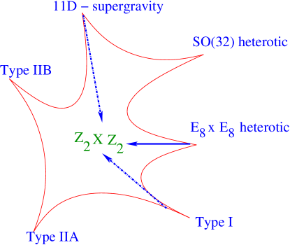
Figure 4: Phenomenological application of M–theory

Figure (4) illustrates qualitatively the approach to the phenomenological application of M–theory proposed in this paper. In this view the different perturbative M–theory limits are used to probe the properties of a specific class of compactifications. In this respect one may regard the free fermionic models as illustrative examples. Namely, in the heterotic limit this formulation highlighted the particular class of models that are connected to the $Z_{2}\times Z_{2}$ orbifold. In order to utilize the M–theory advances to phenomenological purposes, our task then is to now explore the compactification of the other perturbative string limits on the same class of spaces, with the aim of gaining further insight into their properties.

8 Wilsonian matter

The previous sections elaborated on the connection between the simply and non–simply connected manifolds, which is obtained by utilizing the freely acting shifts. This construction enables the GUT symmetry breaking by Wilson lines. In turn, the Wilson line gauge symmetry breaking has far reaching phenomenological and cosmological implications. The important consequence is the appearance of the states in the massless spectrum that do not fit into representations of the original unbroken GUT gauge group. This phenomena is peculiar to Wilson–line symmetry breaking and does not arise in the conventional Higgs symmetry breaking mechanism. Consequently, field theory GUTs do not give rise, in general, to such states. Their appearance is a unique and general consequence of string (M–theory) unification, at least in the heterotic–string limit. I refer to such states as “Wilsonian matter”.

In the free fermionic models the Wilsonian matter arises from sectors that break the $SO(10)$ symmetry, and are produced by combinations of the basis vectors that extend the NAHE set with the NAHE–set basis vectors. The $SO(10)$ symmetry is broken to one of its subgroups, by the assignment of boundary conditions to the set of complex world–sheet fermions ${\bar{\psi}}^{1,\cdots,5}$:

$${b\{{{\bar{\psi}}_{1\over 2}^{1\cdots 5}}\}=\{{1\over 2}~{}{1\over 2}~{}{1\over 2}~{}{1\over 2}~{}{1\over 2}\}\Rightarrow SO(10)~{}\rightarrow~{}SU(5)\times U(1)},~{}~{}~{}$$ (15)

$${b\{{{\bar{\psi}}_{1\over 2}^{1\cdots 5}}\}=\{1~{}~{}1~{}~{}1~{}~{}0~{}~{}0\}\Rightarrow SO(10)~{}\rightarrow~{}SO(6)\times SO(4)}.~{}$$ (16)

To break the $SO(10)$ symmetry to $SU(3)\times SU(2)\times U(1)_{B-L}\times U(1)_{T_{3_{R}}}$ both steps, (15) and (16), are used, in two separate basis vectors. The basis vectors $\{\alpha,\beta,\gamma\}$ that contain the boundary condition assignments eqs. (15,16) correspond to Wilson lines in the orbifold construction.

The spectrum of a free fermionic model then contain states from sectors that do not break the $SO(10)$ symmetry. These typically include the three generations from the twisted sectors $b_{1},~{}b_{2}$ and $b_{3}$; the Higgs multiplets from the untwisted sector and the sector $b_{1}+b_{2}+\alpha+\beta$; and $SO(10)$ singlets. These states obviously fit into $SO(10)$ representations. Additionally, the models contain the states that arise from combinations of the basis vectors that extend the NAHE set. These states can be classified according to the pattern of $SO(10)$ symmetry breaking in each sector. Sectors which break the $SO(10)$ symmetry to $SO(6)\times SO(4)$ or to $SU(5)\times U(1)$ produce states that carry fractional electric charge $\pm 1/2$, which may [21, 47], or may not, be confined by a hidden sector non–Abelian gauge group. Obviously such fractionally charged states should be either confined, sufficiently massive, or sufficiently rare, in order not to conflict with present bounds on the fractionally charged matter. However, as I discuss further below, their appearance is perhaps the most dramatic and interesting consequence of string models. Sectors which break the $SO(10)$ symmetry directly to the Standard Model gauge group also produce states with the standard charges under the Standard Model gauge symmetries, but which carry “fractional” charge under the $U(1)_{Z^{\prime}}$ that is embedded in $SO(10)$ and is orthogonal to the Standard Model weak–hypercharge. Such states can only arise in free fermionic string models in which the $SO(10)$ symmetry is broken directly to the Standard Model gauge group.

The existence of the exotic “Wilsonian matter” in the string models has important phenomenological and cosmological implications. Most important is the fact that it provides an intrinsic stringy mechanism that produces super–heavy meta–stable matter. In the case of the states that carry fractional electric charge the reason is apparent. The lightest fractionally charged state cannot decay into integrally charged matter and is hence stable. More generally, however, we saw in the free fermionic models that the Standard Model states fit into $SO(10)$ representations, whereas there exist exotic Wilsonian states that carry standard charges under the Standard Model gauge group, but carry fractional charge under the $U(1)_{Z^{\prime}}$. Depending on the charges of the Higgs states that break the $U(1)_{Z^{\prime}}$ this case may result in discrete symmetries that forbid, or highly suppress, the decay of the exotic states to the Standard Model states.

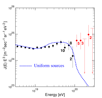
Figure 5: Energy spectrum observed with AGASA [61]

The appearance of exotic “Wilsonian matter” in the string models is intriguing for another reason. One of the most fascinating unexplained experimental observations of recent years is that of Ultra High Energy Cosmic Rays with energies in excess of the Greisen–Zatsepin–Kuzmin (GZK) bound [59]. There are apparently no astrophysical sources in the local neighborhood that can account for the events. The shower profile of the highest energy events is consistent with identification of the primary particle as a hadron but not as a photon or a neutrino. The ultrahigh energy events observed in the air shower arrays have muonic composition indicative of hadrons. The problem, however, is that the propagation of hadrons over astrophysical distances is affected by the existence of the cosmic background radiation, resulting in the GZK cutoff on the maximum energy of cosmic ray nucleons $E_{\rm GZK}\leq 10^{20}\;{\rm eV}$ [60]. Similarly, photons of such high energies have a mean free path of less than 10Mpc due to scattering from the cosmic background radiation and radio photons. Thus, unless the primary is a neutrino, the sources must be nearby. On the other hand, the primary cannot be a neutrino because the neutrino interacts very weakly in the atmosphere. A neutrino primary would imply that the depths of first scattering would be uniformly distributed in column density, which is contrary to the observations. Figure 5 shows the number of events as function of the energy, as observed by the AGASA collaboration [61]. The dotted curve represent the expected fall off of events for extra-galactic sources, because of the GZK cut–off. The AGASA data clearly suggests the observation of events with energies in excess of the GZK cut–off. While this is still a topic of hot debate among the experimentalists, it is without a doubt one of the most intriguing pieces of data that emerged in recent years, and we are well justified in trying to find theoretical explanations of various sorts. Eventually, it is hoped that forthcoming observations by the Pierre Auger [62] and EUSO [63] experiments will resolve the experimental issues.

One of the most intriguing possible solutions is that the UHECR primaries originate from the decay of long–lived super–heavy relics, with mass of the order of $10^{12-15}\;{\rm GeV}$ [64]. In this case the primaries for the observed UHECR would originate from decays in our galactic halo, and the GZK bound would not apply. Furthermore, the profile of the primary UHECR indicates that the heavy particle should decay into electrically charged or strongly interacting particles. From the particle physics perspective the meta–stable super–heavy candidates should possess several properties. First, there should exist a stabilization mechanism which produces the super–heavy state with a lifetime of the order of $10^{17}s\leq\tau_{X}\leq 10^{28}s,~{}$and still allows it to decay and account for the observed UHECR events. Second, the required mass scale of the meta–stable state should be of order, $M_{X}~{}\sim~{}10^{12-13}{\rm GeV}.$

Finally, the abundance of the super–heavy relic should satisfy the relation $({\Omega_{X}/\Omega_{0}})({t_{0}/\tau_{X}})\sim 5\times 10^{-11}\;,~{}$to account for the observed flux of UHECR events. Here $t_{0}$ is the age of the universe, $\tau_{X}$ the lifetime of the meta–stable state, $\Omega_{0}$ is the critical mass density and $\Omega_{X}$ is the relic mass density of the meta–stable state.

As discussed above, superstring theory inherently possesses the ingredients that naturally give rise to super–heavy meta–stable states. The stabilization mechanism arises in string theory due to the breaking of the non–Abelian gauge symmetries by Wilson lines. The massless spectrum then contains states with fractional electric charge or “fractional” charge under the $SO(10)$ $U(1)_{Z^{\prime}}$, which is orthogonal to the weak–hypercharge. The lightest fractionally charged state is stable due to electric charge conservation, and other “Wilsonian states” are meta–stable if their decay to Standard Model states is forbidden by a local discrete symmetry [65]. In practice it is sufficient to demand that vevs which break the discrete symmetry are sufficiently small. The super–heavy states can then decay via the nonrenormalizable operators

$${{\langle V_{1}~{}~{}~{}\cdots~{}~{}~{}V_{N}\rangle}\over{M_{S}^{N-3}}}~{}~{}~{};~{}~{}~{}M_{S}\sim 10^{17-18}{\rm GeV}$$ (17)

which are produced from exchange of heavy string modes. The lifetime of the meta–stable relic is then given by

$$\tau_{X}~{}\approx~{}{1\over{M_{X}}}\left({{M_{S}}\over{M_{X}}}\right)^{2(N-3)}$$ (18)

where $m_{X}$ is the mass of the meta–stable heavy state, $M_{S}$ is the string scale, and $N$ is order of the nonrenormalizable terms. Taking $N=8$, $M_{S}\sim 10^{17-18}\;{\rm GeV}$ and $m_{x}\sim 10^{12}\;{\rm GeV}$, one finds that $\tau_{x}>10^{7-17}\;{\rm years}$ [47].

Additionally, string theory may naturally produce mass scales of the required order, $M_{X}\approx 10^{12-13}{\rm GeV}$. Such mass scales arise due to the existence of an hidden sector which typically contains non–Abelian $SU(n)$ or $SO(2n)$ group factors. Thus, the mass scale of the hidden gauge groups is fixed by the hidden sector gauge dynamics. Therefore, in the same way that the color $SU(3)_{C}$ hadronic dynamics are fixed by the boundary conditions at the Planck scale and the $SU(3)_{C}$ matter content, the hidden hadron dynamics are set by the same initial conditions and by the hidden sector gauge and matter content,

$$M_{X}~{}\sim~{}\Lambda_{\rm hidden}^{\alpha_{s},M_{S}}(N,n_{f}).$$

Finally, the fact that $M_{X}\sim 10^{12-13}{\rm GeV}$ implies that the super–heavy relic is not produced in thermal equilibrium and some other production mechanism is responsible for generating the abundance of super–heavy relic. This may arise from gravitational production [66] or from inflaton decay following a period of inflation.

Next I turn to discuss several specific examples. One particular string theory state that has been proposed as an UHECR candidate is the ’Crypton’, in the context of the flipped $SU(5)$ free fermionic string model. The ‘crypton’ is a state that carries fractional electric charge $\pm 1/2$ and transforms under a non–Abelian hidden gauge group, which in the case of the flipped $SU(5)$ “revamped”string model is $SU(4)$. The fractionally charged states are confined and produce integrally charged hadrons of the hidden sector gauge group, which have been named “tetrons”. The lightest hidden hadron is expected to be neutral with the heavier modes split due to their electromagnetic interactions. A priori, therefore, the ‘crypton’ is an appealing CDM candidate, which is meta–stable because of the fractional electric charge of the constituent ‘quarks’. This implies that the decay of the exotic hadrons can be generated only by highly suppressed non–renormalizable operators (17). Effectively, therefore, the events that generate the UHECR are produced by annihilation of the ‘cryptons’ in the confining hidden hadrons. Moreover, the mass scale of the hidden hadrons is fixed by the hidden sector gauge dynamics, and may naturally be of the order $10^{12-13}{\rm GeV}$. Therefore, in the same way that the color $SU(3)_{C}$ hadronic dynamics are fixed by the boundary conditions at the Planck scale and the $SU(3)_{C}$ matter content, the hidden hadron dynamics are set by the same initial conditions and by the hidden sector matter content. Depending on the order $N$ of the nonrenormalizable tetron–decay mediating operators, the lifetime from Eq. (18) may be in the appropriate range to account for the flux of observed UHECR events above the GZK cutoff [47]. However, in addition to the lightest neutral bound states there exist in this model also long lived meta–stable charged bound states, whose abundance is comparable to that of the neutral states [49]. The reason is that the cryptons, which carry electric charge $\pm 1/2$, are singlets of $SU(2)_{L}$. Therefore, the charged tetrons cannot decay to the neutral tetron by emitting a light $W^{\pm}$ or a light Higgs. Consequently, the charged tetrons can only decay by emitting a massive string state. Effectively, therefore, the only way for the charged tetrons to decay to the neutral one is by the same higher dimensional operators that govern the decay of the neutral tetrons. The lifetime of the charged and neutral tetrons are consequently of similar order. Constraints on the abundance of stable charged heavy matter then places an additional constraint on the lifetime of this form of UHECR candidates. One finds [49] that for a tetron mass $\sim 10^{12}{\rm GeV}$ the tetron density is at most $\Omega_{T}\leq 10^{-6}\Omega_{CDM}\;.$ However, the tetron can still account for the observed UHECR events, provided that $\tau_{T}\leq 2\times 10^{4}t_{U}$, where $t_{U}$ is the age of the universe. Additionally, since the crypton carry fractional $U(1)_{Y}$ charge $\pm 1/2$ and transform as $4$ and $\bar{4}$ of the hidden $SU(4)$ gauge group, it affects the evolution of the weak–hypercharge gauge coupling, but not that of $\alpha_{2}$ or $\alpha_{3}$. Consequently, coupling unification necessitates the introduction of additional matter to achieve unification.

In addition to the fractionally charged states, the free fermionic standard–like models contain states, which arise from $SU(3)\times SU(2)\times U(1)^{2}$ type sectors, and carry the regular charges under the Standard Model, but carry “fractional” charges under the $U(1)_{Z^{\prime}}\in SO(10)$ symmetry. These states can be color triplets, electroweak doublets, or Standard Model singlets and may be good dark matter candidates [28]. The meta–stability of this type of states arises because of their fractional $U(1)_{Z^{\prime}}$ charge. Namely, the fact that the Standard Model states possess the $SO(10)$ embedding, implies that there exist a discrete symmetry which protects the exotic matter from decaying into the lighter Standard Model states. We must additionally insure that the $U(1)_{Z^{\prime}}$ symmetry breaking VEVs, break the discrete symmetry sufficiently weakly. The uniton is such a color triplet that has been motivated to exist at an intermediate energy scale due to its possible role in facilitating heterotic–string gauge coupling unification. It forms bound states with ordinary down and up quarks. The mass of the uniton is generated from nonrenormalizable terms and can be of order $10^{12-13}{\rm GeV}$, as required to explain the UHECR events. Additionally, if the uniton is to contribute substantially to the dark matter, the lightest bound state must be neutral and the heavier charged states must be unstable. However, contrary to the case of the fractionally charged states, the uniton charged bound states can decay through $W^{\pm}$ radiation of the ordinary quark with which it binds. Obviously, the uniton also affects the evolution of the Standard Model gauge couplings. However, a uniton state at intermediate mass scale was motivated precisely because of its effect on the Renormalization Group Equations. Therefore, intermediate mass scale uniton fulfill the dual role of facilitating heterotic–string gauge coupling unification, and at the same time providing a dark matter candidate and a meta–stable super–heavy state that may explain the UHECR events.

Lastly, the free fermionic Standard–like models contain Standard Model singlets that carry fractional $U(1)_{Z^{\prime}}\in SO(10)$ charge. Such states may be semi–stable provided that the discrete symmetry, which suppresses their decay modes, is broken sufficiently weakly. Similar to the states with fractional electric charge, they may transform under a hidden sector non–Abelian gauge group and their mass scale may therefore be fixed by the confining hidden sector dynamics. They do not affect the evolution of the Standard Model gauge couplings, and being neutral, they provide ideal dark matter and UHECR candidates.

9 Blessings in the sky

We observed in the previous section that superstring models provide a variety of candidates, with differing properties, that may account for the observed UHECR events. The phenomenological challenge is to develop the tools that will discern between the different candidates, by confronting their intrinsic properties with the observed spectrum of the cosmic ray showers. The UHECR data, however, opens up new probes to the GUT and string scale physics. The point is that in the analysis of the decay products of the meta–stable states one must extrapolate measured parameters from the low scale, at which they are measured, to the high–scale of the hypothesized meta–stable state. In this extrapolation, which covers more than 10 orders of magnitude in energy scales, one must make some judicious assumptions in regard to the particle content. Thus one may hope that the extrapolation itself will enable to differentiate between different assumptions in regard to the physics in the extrapolation range. This methodology is very similar to that employed successfully in the case of gauge coupling unification in supersymmetric versus non–supersymmetric cases [6]. There the motivation for the extrapolation arises from the hypothesis of unification and one can show that it is consistent only if one includes the supersymmetric spectrum. Similarly, in the case of the UHECR events, the motivation for the high scale are the events themselves and the possibility to explain them with the super–heavy meta–stable matter. The extrapolated parameters are the QCD fragmentation functions and similarly one must include in the evolution whatever physics is assumed to exist in the desert. In ref. [67] supersymmetric fragmentation functions were developed for this purpose. Furthermore, such functions may also be used in the analysis of the cosmic rays showers, which arise from the collision of the primaries with the atmosphere nuclei at a center of mass energies of order $\sim 100{\rm TeV}$.

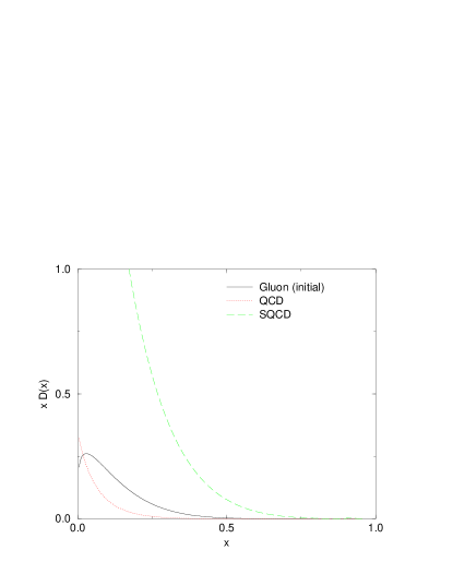
Figure 6: The gluon fragmentation function $xD_{g}^{p,\bar{p}}(x,Q^{2})$ at the lowest scale $Q_{0}=10$ GeV, and its evolved QCD (regular) and SQCD/QCD evolutions with $Q_{f}=$$10^{3}$ GeV. The SUSY fragmentation scale is chosen to be $200$ GeV.

As an illustration of the procedure, consider the decay of a hypothetical 1 TeV massive particle into supersymmetric partons. The decay can proceed, for instance, through a regular $q\bar{q}$ channel, and a shower is developed starting from the quark pair. The $N=1$ DGLAP equation describes in the leading log approximation the evolution of the shower which accompanies the pair. We are interested in studying the impact of the supersymmetric spectrum on the fragmentation. In our runs we have chosen the initial set of Ref. [68]. We parameterize the fragmentation functions as

$$D(x,\mu^{2})=Nx^{\alpha}(1-x)^{\beta}\left(1+\frac{\gamma}{x}\right)$$ (19)

Typical fragmentation functions in QCD involve final states with $p$, $\bar{p}$, $\pi^{\pm},\pi^{0}$ and kaons $k^{\pm}$. We have chosen an initial evolution scale of $10$ GeV and varied both the common SUSY mass scale, $Q_{i}$, and the final evolution scale, $Q_{f}$. In general the effects of supersymmetric evolution are small within the range described by the factorization scales $Q_{f}$ and $Q_{i}$ ($Q_{f}=10^{3}$ GeV, $Q_{i}=200$ GeV).

The situation appears to be completely different for the gluon fragmentation functions. In figure 6 the evolution using the supersymmetric and non–supersymmetric fragmentation functions is displayed. The regular and the SQCD evolved fragmentation functions differ largely in the diffractive region. This will show up in the spectrum of the primary protons if the decaying state has a supersymmetric content. As we raise the final evolution scale we start seeing more pronounced differences between regular and supersymmetric distributions. Comparison of the squark fragmentation functions for all the flavors and the one of the gluino [67] shows that the scharm distribution grows slightly faster than the scalar distributions. The gluino fragmentation function is still the fastest growing at small–x values [67].

The second important scale appearing in the analysis of UHECR concerns the interaction of the primary protons with the nuclei in the atmosphere. These interactions, estimated to be in the several TeV’s, may require a supersymmetric analysis. The supersymmetric evolution of the parton distributions of gluons, squarks and gluinos reveals that the small-x rapid growth of the gluino distribution is visible and points toward an interesting effect in the hadronic cross section of the primaries [67]. Most exciting, however, is perhaps the fact that the forthcoming Pierre Auger and EUSO experiments will explore precisely the physics of the UHECR above the GZK cutoff! The hypothesized meta–stable super–heavy string relics may then serve as experimental probes of the string physics, provided that we are able to develop the phenomenological tools to decipher their predicted properties, such as their fractional electric or $U(1)_{Z^{\prime}}$ charge! Initial efforts in this direction were recently reported in ref. [69].

10 Fundamental principles

Over the past few years important progress has been achieved in the basic understanding of string theories. Under the umbrella of M–theory they are seen to be limits of one fundamental theory. As such M–theory provides the most advanced framework to date to study the unification of the gauge and gravitational interactions. This paradigm led to explicit and detailed models, in the various perturbative limits, and the methodology for confronting those models with experimental data is under intense development. However, should this be the end of the road for M-theory? The answer is obviously not! The story of M–phenomenology, as it pertains to observable phenomena, will not be complete without a rigorous formulation that embarks from well posited basic physics axioms, à la classical, special and general relativity.

It may however be that such a basic formulation requires a revision of the basic formalism of quantum mechanics and quantum field theories. Despite their unprecedented success in the context of the Standard Models, there may exist a fundamental discrepancy between the utilization of the vacuum in quantum field theories, versus what may be needed in the eventual formulation of quantum gravity. In this context, in collaboration with Marco Matone from the University of Padova, we presented a formulation of quantum mechanics starting from an equivalence postulate [70, 71]. I propose that our approach may serve as a starting point for the rigorous formulation of quantum gravity. I recap here briefly the two key ingredients of the formalism whose generalization may yield such a formulation.

The equivalence postulate states that all physical systems labeled by the function ${\cal W}(q)=V(q)-E$, can be connected by a coordinate transformation, $q^{a}\rightarrow q^{b}=q^{b}(q^{a})$, defined by ${\cal S}_{0}^{b}(q^{b})={\cal S}_{0}^{a}(q^{a})$. This postulate implies that there always exist a coordinate transformation connecting any state to the state ${\cal W}^{0}(q^{0})=0$. Classically the state ${\cal W}^{0}(q^{0})=0$ is a fixed point in the space of allowed solutions and therefore the equivalence postulate cannot be implemented consistently. Consistency of the equivalence postulate implies the modification of CM, which is analyzed by a adding a still unknown function $Q$ to the Classical Hamilton–Jacobi Equation. Consistency of the equivalence postulate fixes the transformation properties for ${\cal W}(q)$, ${\cal W}^{v}(q^{v})=\left(\partial_{q^{v}}q^{a}\right)^{2}{\cal W}^{a}(q^{a})+(q^{a};q^{v}),$ and for $Q(q)$, $Q^{v}(q^{v})=\left(\partial_{q^{v}}q^{a}\right)^{2}Q^{a}(q^{a})-(q^{a};q^{v}),$ which fixes the cocycle condition for the inhomogeneous term

$$(q^{a};q^{c})=\left(\partial_{q^{c}}q^{b}\right)^{2}[(q^{a};q^{b})-(q^{c};q^{b})].$$ (20)

The cocycle condition is the first key ingredient in the formalism. It is invariant under Möbius transformations that fix the functional form of the inhomogeneous term. The cocycle condition is generalized to higher, Euclidean or Minkowski, dimensions [71], where the Jacobian of the coordinate transformation extends to the ratio of momenta in the transformed and original systems. A second key ingredient in the formalism is the identity

$$({\partial_{q}{\cal S}_{0}})^{2}=\hbar^{2}/2\left(\{\exp(i2{\cal S}_{0}/\hbar,q)\}-\{{\cal S}_{0},q\}\right)$$ (21)

where $\{,\}$ denotes the Schwarzian derivative, and ${\cal S}_{0}$ is solution of the Quantum Stationary Hamilton–Jacobi Equation. The fundamental characteristic of quantum mechanics in this approach is that ${\cal S}_{0}\neq Aq+B$ always. The equivalence postulate may also shed light on the quantum origin of mass. The generalization of the identity (21) to the relativistic case with a vector potential is,

$$\alpha^{2}(\partial{\cal S}-eA)^{2}={D^{2}(Re^{\alpha{\cal S}})/(Re^{\alpha{\cal S}})}-{\Box R/R}-({\alpha/R^{2}})\partial\cdot(R^{2}(\partial{\cal S}-eA)),$$

where $\alpha=i/\hbar$, $D$ is a covariant derivative, and $\partial\cdot(R^{2}(\partial{\cal S}-eA))=0$ is a continuity condition. The $D^{2}(Re^{\alpha{\cal S}})/(Re^{\alpha{\cal S}})$ term is associated with the Klein–Gordon equation. In this case ${\cal W}(q)=1/2mc^{2}$. From the equivalence postulate it follows that masses of elementary particles arise from the inhomogeneous term in the transformation of the ${\cal W}^{0}(q^{0})\equiv 0$ state, i.e. $1/2mc^{2}=(q^{0};q).$ From this perspective we may speculate that scalar particles and symmetry breaking represent a particular realization of the geometrical transformation $q^{0}\rightarrow q$. Obviously, this interpretation offers new possibilities to understand how particle properties are generated from the vacuum. Consistency of the equivalence postulate also implies tunneling and energy quantization for bound states without assuming the probability interpretation of the wave function, and may therefore offer new perspective on the origin of the Hilbert space structure [70].

The equivalence postulate approach offers a rigorous formalism for quantum mechanics. While its formulation is still in its infancy, we note that the main phenomenological characteristics of quantum mechanics emerge from its consistent implementation. The structure of the formalism is mathematically elegant and rich. The generalization of the two basic ingredients, Eq. (20) and Eq. (21), may eventually yield a rigorous formulation of quantum gravity.

11 Conclusions

Twentieth century particle physics began with the discovery of the the electron by Thompson in 1897. By its end the gauge and matter sectors of the Standard Model have been firmly established. Meanwhile, experimental particle physics evolved from the cathode ray tubes used by Thompson to present day Mega–colliders. In this process, the societies hosting these experiments have been transformed irreversibly, and future impact can be nothing but a speculation.

The Standard Model opened the door to the possibility of realizing Einstein’s dream of finding a unified mathematical framework for the known fundamental matter and interactions. We should not disregard the fact that experimental elucidation of the Higgs mechanism is determinantal to fulfilling this program, and in its lack basic understanding of the origin of mass and the nature of the vacuum is not possible.

The available experimental data strongly indicates the embedding of the Standard Model spectrum in grand unified theories, most elegantly in $SO(10)$. The logarithmic running of the Standard Model gauge and matter parameters is confirmed by experiments, and is in qualitative agreement with high scale unification. Understanding of the Standard Model flavor structure requires unification of the gauge and gravitational interactions. String theories provide the contemporary tools to study this unification.

The development of M–theory transformed our understanding of string theories, which are seen to be limits of a single more fundamental theory. This gives new context to attempts to connect between string theory and experimental data. Indeed numerous studies are underway to construct viable string models by using branes and open string constructions [72, 73]. The approach reviewed in this paper is slightly different. In this view the different string limits can only probe some properties of the true nonperturbative vacuum. Thus, in the heterotic limit the grand unification structures underlying the Standard Model can be seen. On the other hand, the heterotic string is expanded in the zero coupling limit and finite coupling requires moving away from the perturbative heterotic–string limit. Thus, dilaton stabilization might be better addressed in the type I limit. In this respect the fundamental question remains, the selection of the compactified space, out of the myriad of the possibilities, that may correspond to our world. We may regard the string duality picture as allowing us to probe the properties of specific compactifications by compactifying the different limits on the same class of manifolds.

In the heterotic limit the non–Abelian GUT symmetries are broken by Wilson lines, which gives rise to exotic matter. In turn, this exotic matter provides several candidates for dark matter and UHECR events, with differing characteristics. One must therefore develop the tools to decipher their phenomenological properties. Most exciting in this regard is the fact that the Pierre Auger and EUSO experiments are designed to study the physics of UHECR events beyond the GZK cut-off, and some surprises may lie in store!

References

References

- [1] Townsend P K hep-th/9612121; Sen A hep-th/9802051; Duff M J hep-th/9805177; Ovrut B hep-th/0201032.
- [2] Georgi H and Glashow S 1974 Phys. Rev. Lett.32 438.
- [3] Georgi H in Particles and Fields–1974, ed. C.E. Carlson. 1975, New York, AIP Press; Fritzsch H and Minkowski P 1975 Annals Phys. 93 193.
- [4] Witten E 1996 Nucl. Phys. B 471 135; Lykken J 1996 Phys. Rev. D 54 3693; Antoniadis I et al 1998 Phys. Lett. B 436 257; Dienes K R et al 1998 Phys. Lett. B 436 55.
- [5] Georgi H et al1974 Phys. Rev. Lett.33 451.
- [6] Dimopoulos et al 1981 Phys. Rev. D 24 1681; Ellis J et al 1991 Phys. Lett. B 260 131; Langacker P and Luo M 1991 Phys. Rev. D 44 817; Amaldi Uet al 1991 Phys. Lett. B 260 447.
- [7] Chanowitz M et al 77 Nucl. Phys. B 128 506; Buras A J et al 78 Nucl. Phys. B 135 66.
- [8] Candelas P et al 1985 Nucl. Phys. B 258 46; Greene B et al 1987 Nucl. Phys. B 292 606; Arnowitt R and Nath P 1989 Phys. Rev. Lett.62 2225;
- [9] Witten E 1986 Nucl. Phys. B 268 79; Distler J and Kachru S 1994 Nucl. Phys. B 413 213.
- [10] Dixon L et al 1986 Nucl. Phys. B 274 285.
- [11] Narain K S 1986 Phys. Lett. B 169 41; Narain K S et al 1987 Nucl. Phys. B 279 369.
- [12] Font A et al 1990 Nucl. Phys. B 331 421; Casas J A et al 1989 Nucl. Phys. B 317 171.
- [13] Giedt J 2002 Annals Phys. 297 67.
- [14] Kawai K et al 1987 Nucl. Phys. B 288 1; Antoniadis I et al 1987 Nucl. Phys. B 289 87.
- [15] Gepner D 1987 Nucl. Phys. B 290 10; 1988 Nucl. Phys. B 290 757.
- [16] Faraggi A E 1994 Phys. Lett. B 326 62.
- [17] Faraggi A E hep-ph/9707311; hep-th/9910042.
- [18] Dixon L et al 1987 Nucl. Phys. B 282 13; Kalara S et al 1991 Nucl. Phys. B 353 650.
- [19] Dine M et al 1987 Nucl. Phys. B 289 589; Atick J J et al 1987 Nucl. Phys. B 292 109; Cecotti S et al 1987 Int. J. Mod. Phys. A 2 1839.
- [20] Faraggi A E and Nanopoulos D V 1993 Phys. Rev. D 48 3288; Faraggi A E hep-th/9511093; hep-th/9708112.
- [21] Antoniadis I et al 1989 Phys. Lett. B 231 65.
- [22] Antoniadis I et al 1990 Phys. Lett. B 245 161; Leontaris G K and Rizos J 1999 Nucl. Phys. B 554 3.
- [23] Faraggi A E et al 1990 Nucl. Phys. B 335 347; Faraggi A E 1992 Phys. Rev. D 46 3204.
- [24] Faraggi A E 1992 Phys. Lett. B 278 131; 1992 Nucl. Phys. B 387 239.
- [25] Faraggi A E 1992 Phys. Lett. B 274 47; 1995 Phys. Lett. B 377 43; 1996 Nucl. Phys. B 487 55.
- [26] Cleaver G B et al 1999 Phys. Lett. B 455 135; 2001 Int. J. Mod. Phys. A 16 425; 2001 Nucl. Phys. B 593 471; 2000 Mod. Phys. Lett. A 15 1191; 2001 Int. J. Mod. Phys. A 16 3565; 2002 Nucl. Phys. B 620 259.
- [27] Cleaver G B et al 2001 Phys. Rev. D 63 066001; 2002 Phys. Rev. D 65 106003.
- [28] Chang S et al 1997 Phys. Lett. B 397 76; 1996 Nucl. Phys. B 477 65; Elwood J and Faraggi A E 1998 Nucl. Phys. B 512 42.
- [29] Chaudhuri S et al 1996 Nucl. Phys. B 469 357;
- [30] Cleaver G B et al 1998 Nucl. Phys. B 525 3; 1998 Nucl. Phys. B 545 47; 1999 Phys. Rev. D 59 055005; 1999 Phys. Rev. D 59 115003.
- [31] For review see e.g.: Lykken J hep-ph/9511456; Lopez J L hep-ph/9601208; Faraggi A E hep-ph/9404210.
- [32] Abe F et al1995 Phys. Rev. Lett.74 2626; Abachi S et al1995 Phys. Rev. Lett.74 2632.
- [33] Faraggi A E 1993 Nucl. Phys. B 403 101; 1993 Nucl. Phys. B 407 57.
- [34] Antoniadis I et al 1992 Phys. Lett. B 278 257; Faraggi A E and Halyo E 1993 Phys. Lett. B 307 305; 1994 Nucl. Phys. B 416 63; Ellis J et al 1998 Phys. Lett. B 425 86.
- [35] Antoniadis I et al 1992 Phys. Lett. B 279 281; Faraggi A E and Halyo E 1993 Phys. Lett. B 307 311; Faraggi A E and Pati J C 1997 Phys. Lett. B 400 314.
- [36] Antoniadis I et al 1991 Phys. Lett. B 268 188; Antoniadis I et al 1991 Phys. Lett. B 272 31; Faraggi A E 1993 Phys. Lett. B 302 202; Dienes K R and Faraggi A E 1995 Phys. Rev. Lett.75 2646; 1995 Nucl. Phys. B 457 409.
- [37] Faraggi A E 1994 Nucl. Phys. B 428 111; 2001 Phys. Lett. B 499 147; 2001 Phys. Lett. B 520 337; Ellis J et al 1998 Phys. Lett. B 419 123.
- [38] Antoniadis I et al 1990 Phys. Lett. B 241 24; Faraggi A E and Halyo E 1996 Int. J. Mod. Phys. A 11 2357; Faraggi A E and Pati J C 1998 Nucl. Phys. B 526 21; Faraggi A E and Vives O hep-ph/0203061.
- [39] Costa G et al 1988 Nucl. Phys. B 297 244; Hewett J and Rizzo T 1989 Phys. Rep. 183 193; Faraggi A E and Nanopoulos D V 1991 Mod. Phys. Lett. A 6 61; Cvetic M and Langacker P hep-ph/9707451.
- [40] Dedes A and Faraggi A E 2000 Phys. Rev. D 62 016010.
- [41] Faraggi A E 1997 Phys. Lett. B 398 95.
- [42] Faraggi A E 1994 Phys. Lett. B 339 223.
- [43] Faraggi A E and Thormeier M 2002 Nucl. Phys. B 624 163.
- [44] Pati J C, 1996 Phys. Lett. B 388 532.
- [45] Dienes K R and March–Russell J 1996 Nucl. Phys. B 479 113.
- [46] Wen X G and Witten E, 1985 Nucl. Phys. B 261 651; Schellekens A, 1990 Phys. Lett. B 237 363;
- [47] Ellis J et al 1990 Phys. Lett. B 247 257; Ellis J et al 1992 Nucl. Phys. B 373 399; Benakli K et al 1999 Phys. Rev. D 59 047301; Sarkar S and Toldra R 2002 Nucl. Phys. B 621 495.
- [48] Faraggi A E , Olive K A and Pospelov M 2000 Astrophys. J. 13 31.
- [49] Corianò C, Faraggi A E and Plumacher M, 2001 Nucl. Phys. B 614 233.
- [50] Berglund P et al 1998 Phys. Lett. B 433 269; 2002 Int. J. Mod. Phys. A 15 1345.
- [51] Vafa C and Witten E 1996 Nucl.Phys.Proc.Suppl. 46 225; Angelantonj C et al 1999 Nucl. Phys. B 555 116.
- [52] Faraggi A E hep-th/0206165, to appear in PLB.
- [53] Hosotani Y, 83 Phys. Lett. B 126 309; 83 Phys. Lett. B 129 193.
- [54] Donagi R et alhep-th/9901009; hep-th/9912208; Class. Quant. Grav. 17 (2000) 1049.
- [55] Hořava H and Witten E 1996 Nucl. Phys. B 460 506; 1996 Nucl. Phys. B 475 94.
- [56] Faraggi A E et alhep-th/0204080, to appear in NPB.
- [57] Friedman R et al1997 Comm. Math. Phys. 187 679.
- [58] Barr S M 1982 Phys. Lett. B 112 219; Derendinger J P et al 1984 Phys. Lett. B 139 170; Antoniadis I et al 1987 Phys. Lett. B 194 231.
- [59] Hayashida N et al1994 Phys. Rev. Lett.73 3491; Bird D J et al 1994 Astrophys. J. 424 491.
- [60] Greisen K 1996 Phys. Rev. Lett.16 748; Zatsepin G T and Kuzmin V A 1996 Pisma Zh. Eksp. Theor. Fiz. 4 114.
- [61] Takeda M et al1998 Phys. Rev. Lett.81 1163.
- [62] The Auger Collaboration 2002 Nucl.Phys.Proc.Suppl. 110 487.
- [63] Catalano O 2001 Nuovo Cimento 24C 445.
- [64] Berezinsky V, Kachelriess M and Vilenkin A 1997 Phys. Rev. Lett.79 4302; Kuzmin V A and Rubakov V A, 1998 Phys. Atom. Nucl. 61 1028.
- [65] Krauss L M and Wilczek F 1989 Phys. Rev. Lett.62 1221; Faraggi A E 1997 Phys. Lett. B 398 88.
- [66] Chung D J et al 1999 Phys. Rev. D 59 023501.
- [67] Corianò C and Faraggi A E 2002 Phys. Rev. D 65 075001; hep-ph/0106326; hep-ph/0201129.
- [68] Kniehl B A et al 2000 Nucl. Phys. B 582 514.
- [69] Cafarella A et alhep-ph/0208023.
- [70] Faraggi A E and Matone M 1999 Phys. Lett. B 450 34; 1998 Phys. Lett. B 437 369; 1998 Phys. Lett. A 249 180; 1998 Phys. Lett. B 445 77; 1999 Phys. Lett. B 445 357; 2000 Int. J. Mod. Phys. A 15 1869; Faraggi A E hep-th/0003156; Matone M hep-th/0005274.
- [71] Bertoldi G et alhep-th/9909201.
- [72] Aldazabal G et al 2000 JHEP 0002 015; 2001 JHEP 0102 047; Antoniadis I et al 1999 Phys. Lett. B 464 38; 2000 Phys. Lett. B 486 186; Bailin D et al 2001 Phys. Lett. B 502 209; 2002 Phys. Lett. B 530 202; Blumenhagen et al 2000 JHEP 0010 006; 2001 Nucl. Phys. B 616 3; 2002 JHEP 0207 026; Kakushadze et al 1998 Nucl. Phys. B 533 25; Cvetic M et al 2001 Nucl. Phys. B 615 3; hep-th/0206115; Ibanez L E et al 1999 Nucl. Phys. B 542 112; 2001 JHEP 0111 002; Ellis J et alhep-th/0206087; Kokorelis C hep-th/0207234.
- [73] For review and references see e.g.: C. Angelantonj and A. Sagnotti, hep-th/0204089.