Tachyonic Inflation in the Braneworld Scenario

Abstract

We consider cosmological inflation driven by the rolling tachyon in the context of the braneworld scenario. We show that sufficient inflation consistent with the observational constraints can be achieved for well defined upper limits on the five-dimensional mass scale, string mass scale and the string coupling for the bosonic string.

I Introduction

The inflationary scenario offers the attractive possibility of resolving many puzzles of the standard Hot Big Bang cosmology. The crucial feature of most inflationary models is the period of “slow-roll” evolution of a scalar field (the “inflaton”) during which the potential energy dominates the kinetic energy and the universe undergoes a period of exponential expansion. Although particle physics, in particular string theory, provides several very weakly coupled scalar fields which are natural inflaton candidates, at present there exists no clearly preferred inflationary model; it is therefore interesting to explore new possibilities for the inflationary scenario in the early universe.

The study of non-BPS objects such as non-BPS branes, brane-antibrane configurations and spacelike branes has recently attracted great attention given its implications for string/M-theory and cosmology. The conjecture that the classical decay of unstable D-branes leads, in string theory, to a pressureless gas with non-vanishing energy density, and that the vacuum of the tachyon effective action describes a configuration with no D-branes, so that around this minimum there are no physical open string excitations [1], has quickly lead to the idea of a tachyon cosmology [2]. In this scenario, the main idea is to consider the coupling with gravity by adding the Einstein-Hilbert action to the tachyon effective action [2]. From this perspective, it is quite natural to consider the possibility of inflation driven by the rolling tachyon.

Recently, several authors have investigated the cosmological implications of a tachyon rolling down its potential, which depends on the underlying bosonic or supesymmetric theory [3, 4, 5, 6, 7, 8], to its ground state. Tachyonic inflation [9, 10] has also been studied using phenomenological potentials that have not been derived from string theory and can be related to the so called “k-Inflation” [11].

It has been shown by Kofman and Linde [6] that it is very difficult to find realistic inflationary models in the context of string theory tachyon condensation, as it leads to unacceptably large metric perturbations. Also, inflation in these theories occurs only at super-Planckian values of the brane energy density, making the effective four-dimensional gravity theory unreliable near the top of the potential [6].

A natural extention of this proposal is to consider the tachyon as a degree of freedom on the visible three-dimensional brane. Hence, the Einstein-Hilbert action would describe dynamics on the bulk, which is most often considered to be a five-dimensional AdS spacetime background [12]. This proposal implies that, on the brane, the dynamics would be described by the modified Einstein equations [13]. In this work, we will show that these underlying assumptions allow for an inflationary period in which all known observational constraints are successfully met. As we shall see, an important advantage of our proposal is that this period of inflation occurs at the top of the tachyonic potential emerging from the tachyonic effective theory. Also, the brane energy density remains sub-Planckian allowing us to work with the effective four-dimensional gravity theory. Moreover, we find constraints on the fundamental string mass scale $M_{s}$ and the five-dimensional Planck mass, $M_{5}$.

We will show how our approach allows avoiding, to some extent, difficulties with tachyonic inflation [6], even though there is still the serious problem of reheating whose solution does require a better understanding of the couplings of the tachyon to matter [16].

II Tachyonic Inflation

The effective field theory action for the tachyon field $T$ on a $D3$ brane computed in the bosonic String Field Theory (SFT), around the top of the potential, is given by [17]

$$S_{B}=\tau_{3}\int d^{4}x\exp(-T)[l_{s}^{2}\partial_{\mu}T\partial^{\mu}T+(1+T)]~{}~{},$$ (1)

where the normalization factor $\tau_{3}$ is the D3 brane tension

$$\tau_{3}={M_{s}^{4}\over{(2\pi)^{3}g_{s}}}~{}~{},$$ (2)

$g_{s}$ is the string coupling, and the string mass scale is given by $M_{s}^{2}=1/l_{s}^{2}$.

The action given by Eq. (1) is exact up to second order in $\partial_{\mu}T\partial^{\mu}T$ and accounts for the effects of all open string modes. Notice that, with our conventions, the tachyon field $T$ is dimensionless and hence the potential $V(T)=\tau_{3}(1+T)\exp(-T)$ has mass dimension four. Moreover, due to the factor $\exp(-T)$, the kinetic term has a nonstandard form; it is, however, possible to eliminate this factor via a field redefinition

$$\phi=\exp(-T/2)~{}~{},$$ (3)

and hence obtain a canonical kinetic term; in this case, the potential becomes

$$V(\phi)=-\tau_{3}\phi^{2}\log(\phi^{2}/e)~{}~{}.$$ (4)

Now the “stable vacuum” to which the tachyon condenses is at $T\rightarrow\infty$ (or at $\phi=0$) and, for this vacuum, $V^{{}^{\prime\prime}}\rightarrow\infty$ and the tachyon acquires an infinite mass. Hence, with a standard kinetic term for $\phi$, we have a field theory for the tachyon with the property that it rolls down to its stable vacuum and condenses, disappearing from the spectrum as it acquires an infinite mass. This is the manifestation of the disappearance of the whole tower of the open string fields and is consistent with Sen’s conjecture.

One can also write a closed form expression for the action Eq. (1), incorporating all the higher powers of $\partial_{\mu}T$. The effective tachyon field action in Born-Infield form, ignoring the second and higher derivative terms, is described in the presence of gravity by

$$S_{BI}=\tau_{3}\int d^{4}x\sqrt{-g}~{}V(T)\sqrt{1+l_{s}^{2}f(T)\partial_{\mu}T\partial^{\mu}T}~{}~{}.$$ (5)

For small $\partial_{\mu}T$, one can treat the action Eq. (1) as an expansion of action Eq. (5) with $V(T)=(1+T)\exp(-T)$ and $f(T)=2(1+T)^{-1}$. It should, however, be noted that late time evolution of the tachyon field, in either case, does not seem to match the asymptotic behaviour conjectured by Sen. However, we are interested in the early time evolution of the tachyon field, when it is slightly displaced from the top of the potential at $T=0$ (or $\phi=1$), where the time derivatives of the tachyon turn out to be small, and one can safely assume either action (1) or (5). We shall proceed with the action given by Eq. (1) and the field redefinition given by Eq. (3) but it should be noted that, if one uses the action of Eq. (5), with $V(T)$ and $f(T)$ given above, within the slow-roll approximation, the results are the same.

We now show that the potential (4), within the five-dimensional brane scenario, leads to a successful inflationary model.

In the five-dimensional ADS braneworld scenario, the Friedmann equation on the visible brane becomes [13, 14]:

$$H^{2}={\Lambda\over 3}+\left({8\pi\over 3M_{P}^{2}}\right)\rho+\left({4\pi\over 3M_{5}^{3}}\right)^{2}\rho^{2}+{\epsilon\over a^{4}},$$ (6)

where

$$M_{P}=\sqrt{{3\over 4\pi}}{M_{5}^{3}\over\sqrt{\lambda}}~{}~{},$$ (7)

$\lambda$ is the brane tension, which relates the four and five-dimensional Planck scales and the four and five-dimensional cosmological constants via the relationship

$$\Lambda={4\pi\over M_{5}^{3}}\left(\Lambda_{5}+{4\pi\over 3M_{5}^{3}}~{}\lambda^{2}\right)~{}~{}.$$ (8)

Assuming that, as required by observations, the cosmological constant is negligible in the early universe and since the last term in Eq. (6) rapidly becomes unimportant after inflation sets in, the Friedmann equation becomes

$$H^{2} = {8\pi\over 3M_{P}^{2}}\rho\left[1+{\rho\over 2\lambda}\right]$$ (9)

$$= \left(4\pi\over 3M_{5}^{3}\right)^{2}\rho^{2}\left(1+{\rho_{c}\over\rho}\right)~{},$$ (10)

with

$$\rho_{c}={3\over 2\pi}{M_{5}^{6}\over M_{P}^{2}}~{}~{}.$$ (11)

Hence, the new term in $\rho^{2}$ is dominant at high energies, compared to $\lambda^{1/4}$, i.e. $\rho>\rho_{c}$, but quickly decays at lower energies.

Finally, we shall assume that the scalar field is confined to the brane, so that its field equation has the standard form

$$\ddot{\phi}+3H\dot{\phi}+{dV\over d\phi}=0~{}.$$ (12)

The number of e-folds during inflation is given by $N=\int_{t_{\rm i}}^{t_{\rm f}}Hdt$, which becomes [18]

$$N\simeq-(8\tau_{3}l_{s}^{2}){8\pi\over M_{P}^{2}}\int_{\phi_{\rm i}}^{\phi_{\rm f}}{V\over V^{\prime}}\left[1+{V\over 2\lambda}\right]d\phi~{}~{},$$ (13)

in the slow-roll approximation. We see that, as a result of the modification in the Friedmann equation, the expansion rate is increased, at high energies, by a factor $V/2\lambda$.

One can also define the two slow-roll parameters [18]

$$\epsilon \equiv {M_{P}^{2}\over 16\pi}{1\over{8\tau_{3}l_{s}^{2}}}\left({V^{\prime}\over V}\right)^{2}{1+{V/\lambda}\over(2+{V/\lambda})^{2}}~{}~{},$$ (14)

$$\eta \equiv {M_{P}^{2}\over{8\pi}}{1\over{8\tau_{3}l_{s}^{2}}}{V^{\prime\prime}\over V}{1\over 1+{V/2\lambda}}~{}~{}.$$ (15)

Notice that both parameters are suppressed by an extra factor $\lambda/V$ at high energies and that, at low energies, $V\ll\lambda$, they reduce to the standard form. The extra factor $1/8\tau_{3}l_{s}^{2}$ appears in the expressions for $N,\epsilon$ and $\eta$ due to the presence of the factor $\tau_{3}l_{s}^{2}$ in the kinetic energy term in Eq. (1).

The value of $\phi$ at the end of inflation can be obtained from the condition

$${\rm max}\{\epsilon(\phi_{F}),|\eta(\phi_{F})|\}=1~{}~{}.$$ (16)

We shall use the high energy approximation ($V\gg\lambda$) in our calculations which, for the potential Eq. (4), implies

$$M_{5}<\left({1\over{6\pi^{2}g_{s}}}\right)^{1/2}\left({M_{5}\over{M_{s}}}\right)^{-2}M_{P}~{}~{}.$$ (17)

For our model, the slow-roll parameters are given by

$$\epsilon=-{2a(1+\log(\phi^{2}/e))^{2}\over{8\pi\phi^{4}\log^{3}(\phi^{2}/e)}}~{}~{},$$ (18)

$$\eta=-{2a(6+2\log(\phi^{2}/e))\over{8\pi\phi^{4}\log^{2}(\phi^{2}/e)}}~{}~{},$$ (19)

where

$$a\equiv 6\pi^{5}g_{s}^{2}(M_{5}/M_{s})^{6}~{}~{}.$$ (20)

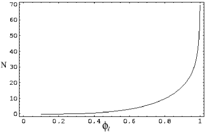
Figure 1: Inflation occurs primarily for initial values of the inflaton field near $\phi=1$, corresponding to the top of the potential.

Table 1: Relevant physical quantities for the tachyonic inflationary potential of Eq. (1), for different values of $a$.

$a$	$\phi_{f}$	$N$	$\phi_{\star}$	$n_{s}$	$r_{s}$	$M_{5}$ (upper bound)	$M_{s}$ (upper bound)
0.28	0.24	70	0.996	0.83	9.7$\times 10^{-5}$	5.6$\times 10^{-3}M_{P}$	1.3$\times 10^{-7}M_{P}$
0.23	0.22	85	0.990	0.86	4.5$\times 10^{-4}$	7.3$\times 10^{-3}M_{P}$	2.6$\times 10^{-7}M_{P}$
0.21	0.22	90	0.988	0.86	6.7$\times 10^{-4}$	7.8$\times 10^{-3}M_{P}$	3.0$\times 10^{-7}M_{P}$
0.20	0.22	96	0.986	0.87	9.7$\times 10^{-4}$	8.3$\times 10^{-3}M_{P}$	3.5$\times 10^{-7}M_{P}$
0.19	0.21	103	0.982	0.88	1.4$\times 10^{-3}$	8.8$\times 10^{-3}M_{P}$	4.1$\times 10^{-7}M_{P}$
0.17	0.21	110	0.978	0.89	2.0$\times 10^{-3}$	9.3$\times 10^{-3}M_{P}$	4.5$\times 10^{-7}M_{P}$
0.15	0.20	129	0.966	0.90	4.1$\times 10^{-3}$	1.1$\times 10^{-2}M_{P}$	6.2$\times 10^{-7}M_{P}$
0.13	0.19	155	0.947	0.92	8.1$\times 10^{-3}$	1.2$\times 10^{-2}M_{P}$	8.0$\times 10^{-7}M_{P}$

The expression for number of e-foldings now becomes

$$N\simeq{8\pi\over{4a}}\int_{\phi_{i}}^{\phi_{f}}{\phi^{3}\log^{2}(\phi^{2}/e)\over{1+\log(\phi^{2}/e)}}d\phi~{}~{}.$$ (21)

For $N\simeq 70$, the minimum number of e-foldings required to solve different cosmological problems, Eqs. (21) and (16) lead to $a\simeq 0.279$ and $\phi_{f}\simeq 0.236$, assuming $\phi_{i}=0.999$. Indeed, we have checked that sufficient inflation can easily be achieved if the field starts very near the top of the potential, at $\phi\simeq 1$ (See Figure 1).

We now turn to the constraints imposed by the observed CMB anistropies. The amplitude of scalar perturbations is given by [18]

$$A_{s}^{2}\simeq 8\tau_{3}l_{s}^{2}{512\pi\over 75M_{P}^{6}}{V_{\star}^{3}\over V_{\star}^{\prime 2}}\left[1+{V_{\star}\over 2\lambda}\right]^{3}~{}~{},$$ (22)

with $V_{\star}=V(\phi_{\star})$, where $\phi_{\star}$ is the value of $\phi$ when scales corresponding to large-angle CMB anisotropies, as observed by COBE, left the Hubble radius during inflation i.e. approximately after 55 e-foldings. For the potential of Eq. (4), again using the high energy approximation, the above equation becomes

$$A_{s}^{2}\simeq{512\pi^{3}\over{4800}}{g_{s}\phi_{\star}^{10}\over{a^{3}}}{\log^{6}(\phi_{\star}^{2}/e)\over{\log^{2}(\phi_{\star}^{2}/e+1)}}~{}~{}.$$ (23)

For our model, with $N_{\star}\approx 55$, $\phi_{i}=0.999$ and $a=0.279$, we get, using Eq. (21)

$$\phi_{\star}\simeq 0.996~{}~{}.$$ (24)

Inserting the above values of $a$ and $\phi_{\star}$ into Eq. (23) and using the fact that the observed value from COBE is $A_{s}\simeq 2\times 10^{-5}$, we get a constraint on $g_{s}$, namely $g_{s}\simeq 1.5\times 10^{-16}$. Using these values of $g_{s}$ and $a$ in Eqs. (17) and (20), we get the following bounds on $M_{5}$ and $M_{s}$:

$$M_{5}\mathrel{\hbox to0.0pt{\lower 4.0pt\hbox{\hskip 1.0pt$\sim$}\hss}\raise 1.0pt\hbox{$<$}}5.6\times 10^{-3}M_{P}~{}~{},~{}~{}M_{s}\mathrel{\hbox to0.0pt{\lower 4.0pt\hbox{\hskip 1.0pt$\sim$}\hss}\raise 1.0pt\hbox{$<$}}1.3\times 10^{-7}M_{P}~{}~{}.$$ (25)

The scale-dependence of the perturbations is described by the spectral tilt [18]

$$n_{s}-1\equiv{d\ln A_{s}^{2}\over d\ln k}\simeq-6\epsilon+2\eta~{}~{},$$ (26)

where the slow-roll parameters are given in Eqs. (14) and (15).

The ratio between the amplitude of tensor and scalar perturbations is given by [15]

$$r_{s}=4\pi\left({A_{t}\over A_{s}}\right)^{2}\simeq{3M_{P}^{2}\over 4}\left({V^{\prime}\over V}\right)^{2}{2\lambda\over V}~{}~{}.$$ (27)

In our model, under the high energy approximation, for $N=70$, we get

$$n_{s}\simeq 0.825~{},$$ (28)

and

$$r_{s}\simeq 9.7\times 10^{-5}~{},$$ (29)

which are within the bounds resulting from the latest CMB data from BOOMERANG [19], MAXIMA [20] and DASI [21], namely

$$0.8<n_{s}<1.05~{}~{}~{},\qquad r_{s}<0.3~{}~{}.$$ (30)

Repeating the above calculations for other values of $a(N)$, we obtain Table 1. We see that, as $a$ decreases, $\phi_{f}$ decreases and $N$, $n_{s}$, $r_{s}$ and $M_{5}$ increase. In all cases, the string remains very weakly coupled ($g_{s}\sim 10^{-16}$) and the string energy density $\tau_{3}$ remains sufficiently below the Planck scale ($\tau_{3}<10^{-12}M_{P}^{4}$) so that one can safely use the low energy four-dimensional gravity theory.

III Conclusions

In this work, we have shown that successful tachyonic inflation can be achieved in the context of a five-dimensional ADS braneworld scenario. We have shown the bosonic SFT action around the top of the tachyon potential does allow a sufficiently long period of inflation provided the string remains very weakly coupled ($g_{s}\sim 10^{-16}$) and the string energy density $\tau_{3}$ is sufficiently below the Planck scale ($\tau_{3}<10^{-12}M_{P}^{4}$) to render the low-energy four-dimensional gravity theory description reliable. Our setup leads to upper bounds on the string scale, typically $M_{s}\mathrel{\hbox to0.0pt{\lower 4.0pt\hbox{\hskip 1.0pt$\sim$}\hss}\raise 1.0pt\hbox{$<$}}8\times 10^{-7}~{}M_{P}$, and on the five-dimensional scale, $M_{5}\mathrel{\hbox to0.0pt{\lower 4.0pt\hbox{\hskip 1.0pt$\sim$}\hss}\raise 1.0pt\hbox{$<$}}10^{-2}~{}M_{P}$ (values of this order seem to be a common feature of inflation on the brane, as they arise in chaotic inflation [22] as well as in supergravity models [23]).

We emphasize that, in our formulation, inflation takes place very close the top of the tachyon potential, thus avoiding the recently identified problem of formation of caustics with multi-valued regions for scalar Born-Infeld theories with arbitrary runaway potentials, meaning that high order spatial derivatives of $T$ become divergent [24].

- [1] A. Sen, “Rolling Tachyon”, hep-th/0203211; “Tachyon Matter”, hep-th/0203265.
- [2] G.W. Gibbons, “Cosmological Evolution of the Rolling Tachyon”, hep-th/0204008.
- [3] M. Fairbairn and M.H. Tytgat, “Inflation from a tachyon fluid?”, hep-th/0204070.
- [4] G. Shiu and I. Wasserman, “Cosmological constraints on tachyonic matter”, hep-th/0205003.
- [5] A. Frolov, L. Kofman and A. Starobinsky, “Prospects and problems of tachyon matter cosmology”, hep-th/0204187.
- [6] L. Kofman and A. Linde “Problems with tachyon inflation”, hep-th/0205121.
- [7] M. Sami, D. Chingangham and T. Qureshi, “Aspects of tachyonic inflation with exponential potential”, hep-th/0205179.
- [8] D. Chaudhuri, D. Ghoshal, D. Jatkar and S. Panda, “On the cosmological relevance of the tachyon”, hep-th/0204204.
- [9] A. Fienstein, “Power-law inflation from the rolling tachyon”, hep-th/0204140.
- [10] T. Padmanabhan, “Accelerated expansion of the universe driven by tachyonin matter”, hep-th/0204150.
- [11] C. Aremendariz-Picon, T. Damour and V. Mukhanov, Phys. Lett. B458, (1999) 209.
- [12] S. Mukohyama, “Brane Cosmology Driven by the Rolling Tachyon”, hep-th/0204084.
- [13] T. Shiromizu, K. Maeda and M. Sasaki, Phys. Rev. D62 (2000) 024012.
- [14] P. Binétruy, C. Deffayet, U. Ellwanger and D. Langlois, Phys. Lett. B477 (2000) 285; E.E. Flanagan, S.H. Tye and I. Wasserman, Phys. Rev. D62 (2000) 044039.
- [15] D. Langlois, R. Maartens and D. Wands, Phys. Lett. B489 (2000) 259.
- [16] J.M. Cline, H. Firouzjahi and P. Martineau, “Reheating from Tachyon Condensation”, hep-th/0207156.
- [17] A. Gerasimov and S. Shatashvili, JHEP , 0010, (2000) 034; D. Kutasov, M. Marino and G. Moore, JHEP , 0010 (2000) 045.
- [18] R. Maartens, D. Wands, B.A. Bassett and I.P.C. Heard, Phys. Rev. D62 (2000) 041301.
- [19] C.B. Netterfield Pryke et al., “A measurement by BOOMERANG of multiple peaks in the angular power spectrum of the cosmic microwave background”, astro-ph/0104460.
- [20] A.T. Lee et al., “A High Spatial Resolution Analysis of the MAXIMA-1 Cosmic Microwave Background Anisotropy Data”, astro-ph/0104459.
- [21] C. Pryke, et al., “Cosmological Parameter Extraction from the First Season of Observations with DASI”, astro-ph/0104490.
- [22] M.C. Bento and O. Bertolami, Phys. Rev. D65 (2002) 063513.
- [23] M.C. Bento, O. Bertolami and A.A. Sen, “Supergravity Inflation on the Brane”, gr-qc/0204046.
- [24] G. Felder, L. Kofman and A. Starobinsky, “Caustics in Tachyon Matter and Other Born-Infeld Scalars”, hep-th/0208019.