A Note on the Positive Constant Curvature Space
Abstract
We construct a positive constant curvature space by identifying some points along a Killing vector in a de Sitter Space. This space is the counterpart of the three-dimensional Schwarzschild-de Sitter solution in higher dimensions. This space has a cosmological event horizon, and is of the topology , where denotes a -dimensional conformal Minkowski spacetime.
In recent years people have been paying particular interest on the constant curvature spacetimes. For the case of negative constant curvature space, namely the anti-de Sittter (AdS) space, it should be mainly attributed to the celebrated AdS/CFT (conformal field theory) correspondence [1], which states that the string or M theory on an AdS space times a compact space is dual to a strong coupling conformal field theory residing on the boundary of the AdS. For the case of positive constant curvature space, namely the de Sitter (dS) space, one of the reasons responsible for the particular interest is that defined in a manner analogous to the AdS/CFT correspondence, an interesting proposal, which says that there is a dual between quantum gravity on a dS space and a Euclidean CFT on a boundary of the dS space, the so-called dS/CFT correspondence, has been suggested recently [2]. Another reason is that our universe may be an asympotically dS spacetime [3]. However, different from the cases for the asymptotically flat or AdS spacetimes, we have not yet a fundamental description of asymptotically dS spacetimes in the sense of quantum gravity: there is presently no fully satisfactory embedding of dS space into string theory [4].
In dimensions, the AdS space has the topology . By identifying points in the universal covering space of the AdS space in a some manner, one can construct various spacetimes which are locally equivalent to the AdS space. It is well-known that the BTZ black hole [5] just belongs to this kind of spacetime, which is constructed by identifying points along a boost Killing vector in a three dimensional AdS space. Its counterparts are discussed in four dimensions [6] and in higher dimensions [7], respectively. The topology structure of the BTZ black hole is , where denotes a conformal Minkowski spacetime in dimensions. So the topology of the BTZ black hole is not peculiar, but its higher dimensional counterparts have the topology in the case of dimensions, which is quite different from the usual one . These black holes look strange in the sense that the exterior of black holes is time-dependent and there is no globally defined timelike Killing vector in the geometry of these black holes [8]. So it is quite difficult to discuss the thermodynamics associated with the black hole. In spite of the peculiar feature of the black hole geometry, in [9] we applied the surface counterterm approach to a five dimensional constant curvature black hole, and obtained the stress-energy tensor of dual conformal field theory. For other methods to study the constant curvature black holes, see [7, 10].
On the other hand, a -dimensional dS space has the topology . Different from the AdS case, the dS space has a cosmological horizon and associated Hawking temperature and thermodynamic entropy [11]:
| (1) |
where is the gravitational constant in dimensions, is the radius of dS space and denotes the volume of a -dimensional unit sphere. Due to this, it is argued that the dS space should be described by a theory with a finite number of independent quantum states; the cosmological constant should be understood as a direct consequence of the finite number of states in the Hilbert space describing the world [12, 13, 14]. Thus a natural consequence is that a necessary condition for a (coarse-gained) spacetime to be described by a theory with states is that the entropy accessible to any observer in that spacetime must obey [4]
| (2) |
According to the “ correspondence” [13], the theory with states may describe the set all of spacetimes: the class of spacetimes with positive cosmological constant , irrespective of asymptotic conditions and types of the matter present [4]. Applying the condition (1) to the candidate set all, a suggestion named “N bound” has been proposed in [13], which in four dimensions states: In any universe with a positive cosmological constant (as well as arbitrary additional matter that may well dominate at all times) the observable entropy is bounded by . Roughly specking, the “N bound” means that the observable entropy in the spacetimes with a positive cosmological constant must be less than or equal to the entropy (1). This “N bound” leads naturally to the Bekenstein entropy bound of matter in dS spaces [15]. The geometry of the dS space looks simple, but this space has much non-trivial physics.
Similar to the negative constant curvature case, in this note we construct a positive constant curvature spacetime by identifying points along a rotation Killing vector in a dS space. Our solutions turns out to be counterparts of the three-dimensional Schwarzschild-dS solution in higher dimensions, and have an associated cosmological horizon. There is a parameter in the solution, which can be explained as the size of cosmological horizon.
Let us begin with the five dimensional case. A five dimensional dS space can be understood as a hypersurface embedded into a six dimensional flat space, satisfying
| (3) |
where is the radius of the dS space. This dS space has fifteen Killing vectors, five boosts and ten rotations. Consider a rotation Killing vector with norm , where is an arbitrary real constant. The norm is always positive or zero. In terms of the norm, the hypersurface (3) can be expressed as
| (4) |
From (4) we see that when , the hypersurface reduces to a null one
| (5) |
while , it goes to a hyperboloid
| (6) |
The null surface (5) has two pointwise connected brances, called and , described by
| (7) | |||||
| (8) |
The hyperboloid (6) has two connected surfaces, named and , defined as
| (9) | |||||
| (10) |
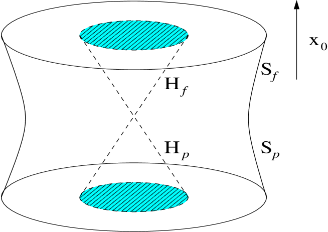
We plot the dS space in Fig. 1. Each point in the figure represent a pair and with fixed. On the surfaces and , we have , while on the surfaces and of the two cones. In the region between and , one has , and inside the two cones. Thus an observer located at the surface or cannot see events which happen inside the cone with null surface or . That is, there does not exist any communication between the inside the cones and outside the cones. Therefore, the surface can be regarded as the future cosmological event horizon and as the past one.
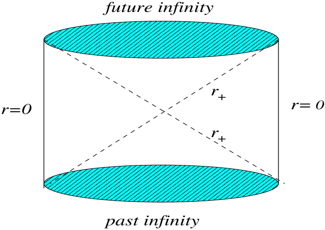
Identifying points along the Killing vector , another one-dimensional manifold becomes compact and isomorphic to . Thus we finally obtain a spacetime with cosmological horizon and with the topology . The Penrose diagram of the positive constant curvature spacetime is plotted in Fig. 2. Similiar to the case of negative constant curvature [7], we may describe the spacetime in the region with by introducing six dimensionless local coordinates ,
| (11) | |||
| (12) | |||
| (13) |
where
| (14) |
Here the coordinate range is , and with the restriction in order to keep positive. In coordinates (11), the induced metric is
| (15) |
which has the same form as the case of negative constant curvature [7]. However, it should be pointed out here that the coordinates (11) and the definition of are different from the corresponding ones in the constant curvature black holes. In these coordinates it is evident that the Killing vector is with norm . Thus in these coordinates one has on the surfaces and and on the horizons and . With the identification , the solution has obviously the topology .
It is trivial to generalize the five dimensional case to other dimensions. For the case of an arbitrary dimensions (), the dS space is a hypersurface satisfying
| (16) |
in a -dimensional flat spacetime. Consider a rotation Killing vector with norm and identify points along the orbit of this Killing vector, we can obtain a positive constant curvature space with the topology . Introducing dimensionless coordinates like (11), one has the induced metric
| (17) |
where and .
Like the dS space, we can also introduce Schwarzschild coordinates to describe the solution. Using local “spherical” coordinates defined as
| (18) | |||
| (19) |
where , and the coordinate range is , and , we find that the solution can be expressed as
| (20) |
where and
| (21) |
In these coordinates is the cosmological horizon. This solution is just the counterpart of a five dimensional constant curvature black hole in the Schwarzschild coordinates [7]. The only difference is that there is replaced by here. In three dimensions, the corresponding induced metric is
| (22) |
After a suitable rescaling of coordinates it can be transformed to usually three-dimensional Schwarzschild-de Sitter solution [16]. In (21), if , it also reduces to the three-dimensional Schwarzschild-dS solution.
Within the cosmological horizon dS space is time-independent in the static coordinates. The solution (20) looks also static, but it does not cover the whole region within the cosmological horizon, which can be seen from the definition of coordinates (18) because they must obey the constraint: ,
As the black hole case, there is a set of coordinates which cover the whole region within the cosmological horizon. They are [9]
| (23) | |||
| (24) |
In terms of these coordinates, the solution is described by
| (25) |
where and
| (26) |
It can be seen from (26) that when , the solution will reduce to the three-dimensional Schwarzschild-dS solution (22). Therefore the solution we constructed here is the counterpart of the three-dimensional Schwarzschild-dS spacetime in five dimensions. Further it should be emphasized here that both sets of coordinates (18) and (23) can be used within the cosmological horizon only. This can be seen from the metrics (20) and (25): beyond the horizon the signature of the solution changes. It is certainly of interest to find a set of coordinates describing the outer region of cosmological horizon.
In dimensions, the solution is
| (27) |
where is still the one given before, and
| (28) |
Here denotes the line element of a -dimensional unit sphere.
The Euclidean sector of the solution can be obtained via the transformation, , in the solution (25). In that case, the line element (26) is changed to
| (29) |
In order the to describe a regular three-sphere, the must have a range with
| (30) |
In the coordinates (18), the Euclidean sector of the solution is (20) with
| (31) |
here has the range with
| (32) |
which differs from the value of (30). Although the solution expressed in terms of the coordinates (18) does not cover the whole interior of cosmological horizon, the Euclidean sector of solution is complete in both sets of coordinates (18) and (23). Further, regarding or as the inverse temperature of the cosmological horizon seems problematic since calculating the surface gravity of the cosmological horizon shows it does not satisfy the usual thermodynamic relation . Obviously, it is of great interest to discuss the thermodynamics associated with the cosmological horizon in the constructed spacetime.
Next we further consider the Euclidean solution in the coordinates (29). Making a coordinate transformation and , one can find that the Euclidean solution (25) with (29) can be expressed as
| (33) |
This is evidently the Euclidean solution of de Sitter space in the static coordinates with the Euclidean time . Since the has the period , so the solution (33) does not describe a regular instanton. The regular instanton requires the Euclidean time has a period . This implies that the solution (25) has a conical singularity along the circle if with a deficit angle . When , the deficit angle is less than , otherwise it becomes negative. When , the solution is regular without any singularity. This situation is the same as the case of three dimensional Schwarzschild-dS solution [16].
In summary we have constructed a positive constant curvature space by identifying points along a rotation Killing vector in a dS space. This space is the counterpart of the three-dimensional Schwarzschild-dS solution in higher dimensions. Also this space can be viewed as corresponding counterpart of the negative constant curvature black hole constructed in [7]. Unlike the dS space, the positive constant curvature space constructed in this note has the topology . As the dS space, however, it still has a cosmological horizon . The solution has a conical singularity along the circle if . It should be interesting to discuss the thermodynamics of cosmological horizon and dual conformal field theory in the spirit of dS/CFT correspondence.
Acknowledgments
The author thanks H.Y. Guo and J.X. Lu for useful discussions, and C.T. Shi for help in drawing the figures. This work was supported in part by a grant from Chinese Academy of Sciences.
REFERENCES
- [1] J. M. Maldacena, Adv. Theor. Math. Phys. 2, 231 (1998) [Int. J. Theor. Phys. 38, 1113 (1999)] [arXiv:hep-th/9711200]; S. S. Gubser, I. R. Klebanov and A. M. Polyakov, Phys. Lett. B 428, 105 (1998) [arXiv:hep-th/9802109]; E. Witten, Adv. Theor. Math. Phys. 2, 253 (1998) [arXiv:hep-th/9802150].
- [2] A. Strominger, arXiv:hep-th/0106113; M. Spradlin, A. Strominger and A. Volovich, arXiv:hep-th/0110007.
- [3] A. G. Riess et al. [Supernova Search Team Collaboration], Astron. J. 116, 1009 (1998) [arXiv:astro-ph/9805201]; S. Perlmutter et al. [Supernova Cosmology Project Collaboration], Astrophys. J. 483, 565 (1997) [arXiv:astro-ph/9608192]; R. R. Caldwell, R. Dave and P. J. Steinhardt, Phys. Rev. Lett. 80, 1582 (1998) [arXiv:astro-ph/9708069]; P. M. Garnavich et al., Astrophys. J. 509, 74 (1998) [arXiv:astro-ph/9806396].
- [4] R. Bousso, O. DeWolfe and R. C. Myers, arXiv:hep-th/0205080.
- [5] M. Banados, C. Teitelboim and J. Zanelli, Phys. Rev. Lett. 69, 1849 (1992) [arXiv:hep-th/9204099]; M. Banados, M. Henneaux, C. Teitelboim and J. Zanelli, Phys. Rev. D 48, 1506 (1993) [arXiv:gr-qc/9302012].
- [6] S. Aminneborg, I. Bengtsson, S. Holst and P. Peldan, Class. Quant. Grav. 13, 2707 (1996) [arXiv:gr-qc/9604005].
- [7] M. Banados, Phys. Rev. D 57, 1068 (1998) [arXiv:gr-qc/9703040]; M. Banados, A. Gomberoff and C. Martinez, Class. Quant. Grav. 15, 3575 (1998) [arXiv:hep-th/9805087].
- [8] S. Holst and P. Peldan, Class. Quant. Grav. 14, 3433 (1997) [arXiv:gr-qc/9705067].
- [9] R. G. Cai, Phys. Lett. B 544, 176 (2002) [arXiv:hep-th/0206223].
- [10] J. D. Creighton and R. B. Mann, Phys. Rev. D 58, 024013 (1998) [arXiv:gr-qc/9710042].
- [11] G. W. Gibbons and S. W. Hawking, Phys. Rev. D 15 (1977) 2738.
- [12] T. Banks, arXiv:hep-th/0007146.
- [13] R. Bousso, JHEP 0011, 038 (2000) [arXiv:hep-th/0010252].
- [14] W. Fischler, 2000, unpublished; Taking de Sitter seriously. talking given at Role of scaling Laws in Physics and Biology (Celebrating the 60th birthday of Geoffrey West), Santa Fe, Dec. 2000; also see the review paper hep-th/0203101 by R. Bousso.
- [15] R. Bousso, JHEP 0104, 035 (2001) [arXiv:hep-th/0012052]; R. G. Cai, Y. S. Myung and N. Ohta, Class. Quant. Grav. 18, 5429 (2001) [arXiv:hep-th/0105070].
- [16] S. Deser and R. Jackiw, Annals Phys. 153, 405 (1984); M. I. Park, Phys. Lett. B 440, 275 (1998) [arXiv:hep-th/9806119].