Obstruction to D-brane Topology Change

Abstract:

A study of the relation between topology change, energy and Lie algebra representations for fuzzy geometry in connection to $M$-theory is presented. We encounter two different types of topology change, related to the different features of the Lie algebra representations appearing in the matrix models of $M$-theory. From these studies, we propose a new method of obtaining non-commutative solutions for the non-Abelian $D$-brane action found by Myers. This mechanism excludes one of the two topology changing processes previously found in other non-commutative solutions of many matrix-based models in $M$-theory i.e. in M(atrix) theory, Matrix string theory and non-Abelian $D$-brane physics.

1 Introduction

During the last few years we have seen how non-commutative geometry has come to play an important role in string theory. It appears not only at the fundamental Planck distances where a smooth geometry cannot be trusted, but also at the level of effective theories in $D$-brane physics, where the Chan-Paton factors result in matrix degrees of freedom. In these cases the effective Lagrangian of $N$ $Dp$-branes comes with built-in non-commutative features in the form of matrix models. Myers [1] proposed an effective action for these non-Abelian $D$-branes by demanding consistency with $T$-duality among the different $Dp$-branes. In particular, he started from the well-known $D$9-brane action and proceeded by $T$-dualizing. The agreement with the weak background actions of Taylor and Van Raamsdonk [2] was used as a consistency check. Note that these linearized actions came from a very different theoretical framework associated with the BFSS M(atrix) theory proposal [3].

This remarkable characteristic of the built-in non-commutativity is not new in the framework of $M$-theory. We already have at least two other examples where this type of construction is found, namely M(atrix) theory [3] and Matrix string theory [4, 5, 6, 7]. In the first case all the configurations of the theory are to be found in terms of matrix degrees of freedom, including the fundamental strings and $D$-branes. In the second case, we have a new formalism in which a two-dimensional action naturally includes matrix degrees of freedom representing the ‘string bits’, which also incorporate the description of higher dimensional objects of $M$-theory using non-commutative configurations.

One of the important properties of this new theoretical framework (Non-Abelian $Dp$-branes, M(atrix)-theory, Matrix string theory) lies in the similarity of the mathematical language used to describe the fundamental objects of $M$-theory, bringing for the first time the possibility of describing strings and $D$-branes in a unified framework, a “democracy of $p$-branes” [9].

An essential characteristic of the matrix actions is their capability to describe non-commutative geometries that correspond to different extended objects of the theory. For example, higher dimensional $Dq$-branes may be formed by smaller $Dp$-branes ($q>p$). To be more precise, consider the dielectric effect [1] where $N$ $Dp$-branes form a single $D{(p+2)}$-brane generating a configuration corresponding to a non-commutative two-sphere (fuzzy sphere [10, 11, 12]). Another kind of construction corresponds to $N$ $D$1-branes forming $n$ $D$5-branes ($n<N$), this time using a fuzzy four-sphere [15]. Also it is worth mentioning that there are other non-commutative manifolds (apart from the fuzzy $n$-spheres) which are relevant to matrix models, e.g. fuzzy versions of tori, $CP(n)$, $RP(n)$, etc.

In this work we will study the relations between the discrete partonic picture (the non-commutative picture) and the smooth geometry that is obtained from it in the limit of large number of partons, i.e. the “reconstruction” of the geometry. Basically, we would like to understand what is the relation between the matrix representation of the partonic picture and the resulting commutative manifold. This relation should be independent of the $M$-theory object we are using as the fundamental parton once we invoke the “$p$-brane democracy idea”.

In particular, we will be working with non-Abelian $D$-brane actions. In section 2 we will show the constraints that these classical actions impose on the set of possible algebraic structures appearing as solutions of the corresponding equations of motion. Also we will explain the mechanism of obtaining the fuzzy geometries (quantum geometries) and the reconstruction of the corresponding commutative manifolds (classical geometries). We will also discuss how the energy of the different configurations are crucial to obtain the commutative geometry in the classical limit. We identify two different types of topology change occurring in these matrix-valued models. In section 3 we consider a new mechanism of fixing the geometry by breaking the symmetry between the solutions of the equations of motion representing quantum geometries.

The main result is a new class of non-commutative $D$-brane solutions with obstruction to topology change. It is based on the important role played by the symmetric representations of the Lie algebra structure underlying these solutions. We also identify two types of topology change that can occur in these effective descriptions.

2 Quantum vs Classical geometry

In this section we summarize the characteristics that define the non-commutative solutions found in non-Abelian $D$-brane physics which are importatant for us.

Let us first give a simple example of how to find quantum geometries. Following this, it will be easier to discuss the more general approach. In the original calculation [1], Myers considered $N$ $D$0-branes in a constant four-form Ramond-Ramond (RR) field strength background of the form $F^{(4)}_{t123}=-2f\epsilon_{123}$. The relevant $D$0-brane action is given by

$$S_{Do}=\mu_{0}\lambda^{2}\int{dt\;{\rm Tr}\left({1\over 2}\partial_{t}\Phi^{i}\partial_{t}\Phi_{i}-{1\over 4}[\Phi^{i},\Phi^{j}][\Phi_{j},\Phi_{i}]+{i\over 3}F^{(4)}_{tijk}\Phi^{i}\Phi^{j}\Phi^{k}\right)},$$ (1)

where $\Phi^{i}$ are complex matrix-valued scalars. They represent the nine directions $i=1,2,..,9$ transverse to the $D$0-brane. $\mu_{0}$ is the charge of the $D$0-brane and $\lambda=2\pi\alpha^{\prime}$ ($\alpha^{\prime}$ has dimension $({\rm length})^{2}$). For static configurations, the kinetic term vanishes and center-of-mass degrees of freedom decouple. Hence, variation of the action gives the following polynomial equation in $\Phi$,

$$[\Phi^{j},[\Phi^{j},\Phi^{i}]]+if\epsilon_{ijk}[\Phi^{j},\Phi^{k}]=0$$ (2)

where indices are contracted with flat Euclidean metric.

This is solved by setting to zero all but the first three scalars $\Phi^{i}$ ($i=(1,2,3)$) which are replaced by Lie algebra generators $T^{i}$ (in this case angular momentum operators) times a scalar $r$. Then the above equation becomes an equation for $r$,

$$r-f=0.$$ (3)

Therefore, three of the scalars $\Phi^{i}$ are of the form $\Phi^{i}=fT^{i}$. The non-commutative geometry appears since these $\Phi$ also correspond to the first three cartesian coordinates transverse to the brane.

However, as explained in appendix B, the above equations do not fully define the quantum geometry. It is still necessary to fix the representation of $T^{i}$ as different representations give different solutions and topologies. Each of these solutions has a characteristic energy $E$, that is a function of the quadratic Casimir as given by

$$E=-{\mu_{0}\lambda^{2}f^{2}\over 6}\sum^{3}_{i=1}\hbox{Tr}[\Phi^{i}\Phi^{i}].$$ (4)

Given a fixed size of the representation $N$, the irreducible representation corresponds to the lower bound (strictly speaking this is the fuzzy sphere), while the reducible representations have higher energies corresponding to more complicated topologies of the direct sums of fuzzy spheres. An important characteristic of the above construction is that in the large $N$ limit the algebra of “functions” defined by these solutions becomes the algebra of functions on the classical manifold (see appendix B).

This example contains all of the ingredients that define the process of finding the non-commutative solutions. Generalizations of this program have appeared, but the underlying structure is the same. These solutions are usually called “fuzzy spaces”, although not all of them are properly well-defined, the best-known such example being the so-called fuzzy four-sphere

In any case, we can now describe the general picture in terms of the following basic steps:

• The starting point is the non-Abelian action of $N$ $Dp$-branes in the presence of non-trivial background and world-volume fields.

• This action is expanded in terms of the polynomials of the scalar fields $\Phi^{i}$ and their world-volume derivatives, where each monomial comes with a symmetric and/or skew-symmetric product of the $\Phi^{i}$’s which translates into commutator and anti-commutator expressions. The background fields are being understood as couplings of the world-volume theory.

• The equations of motion therefore involve a set of polynomials in $\Phi^{i}$ containing their commutators and anti-commutators.

• Then, one identifies a subset of the $\Phi^{i}$’s with some elements of a Lie algebra times a function $r$ commuting with the Lie algebra elements. The idea is that the algebraic structure will take care of the commutators and anti-commutators while $r$ will solve the remaining equations (possibly differential equations in the world-volume variables).

• Finally, one finds different solutions for the field $r$ corresponding to each of the different representations of the Lie algebra generators identified with the $\Phi^{i}$’s. Each of the different representations encode different topologies and geometries.

We emphasize two important aspects in the above program. First, the representations associated with scalars $\Phi^{i}$ are not fixed by the equations of motion. Second, the possibility of topology change is suggested by the natural decay of higher energy solutions into lower energy ones. This cascade process has already received some attention in [17], the main result being the discovery of unstable modes that trigger the topology change. These modes are related to the relative positions of the different fuzzy manifolds that appear in the higher energy solutions: given a solution $A$, we can always construct another solution (of higher energy and more complicated topology) by considering larger matrices of two or more copies of $A$. The different topologies of the above types of solutions come from the fact that they correspond to reducible representations.

Nevertheless, it is important to note that this is not the only way of obtaining topology change. There is also the possibility of having different quantum geometries defined in the same group structure, which are not related by the simple “reducible-irreducible” relations. For example, $SU(4)$ contains many different fuzzy geometries among which we have $CP(3),CP(2)$ and $S^{2}\times S^{2}$ (see appendix B).

Regarding these aspects, it is obvious that if the representation is fixed by the equations of motion, there is no room for topology change. The fact that we can choose the representation signals the existence of a degeneracy in the set of quantum geometries, a symmetry that allows topology change. What we have seen in this section is that from the point of view of the $D$-brane physics, the equations of motion only define the group structure, while energy is (in all of the solutions found until now) the only quantity that differentiates between quantum geometries and therefore “chooses” the classical geometry in the large $N$ limit via the decay processes.

Therefore, we have a clear relation between topology change and the fact that the equations of motion do not fix the representation of the group. Although all of the solutions that are currently known share the latter feature, there is no reason to believe that there are no circumstances in which the equations of motion fix the representation uniquely and hence preclude topology changing processes. To investigate this matter we need to understand in greater depth the definition of fuzzy geometry and the relations between fuzzy coordinates, representations and invariants of the algebraic structure.

An intuitive way to understand a fuzzy geometry is to define it by a deformation of the algebra of functions in classical geometry. For example, take the functions on the sphere. It is enough to consider the spherical harmonics. In a classical case there is an infinite number of these. Now, truncate the basis at a given angular momentum $j$ by projecting out all the higher angular momentum modes. The resulting algebra (with $*$-product replacing point-wise multiplication) represents the fuzzy sphere (see [10, 11, 12] and references therein).

An important mathematical point is that this algebra of functions can be obtained from the symmetric irreducible representations of size $2j+1=N$ of $SU(2)$ using coherent-state techniques (see appendix B). Actually, there exists a precise relation between Cartesian coordinates in $R^{3}$ (which defines the embedding of the sphere in $R^{3}$) and the $SU(2)$ Lie algebra generators in the corresponding representation. The latter are the three matrices $T^{i}$ appearing in the dielectric effect of Myers (note that ${\rm Tr}(T^{i}T^{i})=NR^{2}$, with $R$ equal to the radius of the fuzzy sphere in a suitable length unit).

Nevertheless, the sphere is a sort of a degenerate case since skew-symmetric representations are trivial for $SU(2)$ and there are only two basic tensor invariants, corresponding to the structure constants and Cartan metric. In constructions related to higher rank groups like $SU(n)\ (n\geq 3)$, there are more tensor invariants and the skew-symmetric representations are non-trivial, giving more interesting structures.

An interesting generalization of the fuzzy sphere with rich enough algebraic structure is the 2$n$-dimensional fuzzy complex projective planes (fuzzy $CP(n)$) [18]. These quantum geometries are strongly related to $SU(n)$. It turns out that to define fuzzy $CP(n)$, the equation

$$d_{ijk}T^{j}T^{k}=w\,T^{i},$$ (5)

is sufficient, where $d_{ijk}$ is the usual invariant rank three symmetric tensor for $SU(n)\ (n\geq 3)$, and $w$ depends in particular on the representation used. This equation will play an important role in the next section.

3 Model with Obstruction to Topology Change

In this section we show how to find a concrete example where the $D$-brane equations of motion include an invariant tensorial equation, (like equation 5) that determines the representation and hence enforces an obstruction to topology change. In doing so we will use (5) as a hint and will search for a simple configuration where fuzzy $CP(2)$ could appear.

In order to do this, consider $N$ $D$1-branes with a constant world-volume electric field $F_{\tau\sigma}$ (the $F_{[2]}$ in what follows) in the presence of a five-form RR field strength $F_{ijklm}$ (the $F_{[5]})$), flat metric, constant dilaton and zero B-field. The energy density for this system is obtained by expanding the non-Abelian action proposed by Myers followed by the Legendre transformation. Here we show the final form for the energy density, once we have restricted our study to static and constant configurations:

$$E(\Phi,F_{[2]},F_{[5]}) = \mu_{1}\lambda^{2}\left[{1\over 4}\Phi^{ij}\Phi_{ji}-{1\over 4}F^{2}_{\tau\sigma}\right]+$$ (6)

$$+\mu_{1}\lambda^{4}\left[{1\over 16}(\Phi^{ij}\Phi_{ji})^{2}-{1\over 8}\Phi^{ij}\Phi_{jk}\Phi^{kl}\Phi_{li}-{1\over 16}F^{2}_{\tau\sigma}\Phi^{ij}\Phi_{ji}+\right.$$

$$\hskip 113.81102pt\left.+{1\over 10}\Phi^{i}\Phi^{j}\Phi^{k}\Phi^{l}\Phi^{m}F_{mlkji}F_{\tau\sigma}\right].$$

Here we have used the convention $\Phi^{ij}=[\Phi^{i},\Phi^{j}]$, $i,j...\in[1,2,..,8]$. This expression is bounded from below since the term proportional to $\Phi_{ij}^{2}$ is positive and grows faster then any other with the size of the representation in which $\Phi^{i}$ is. We also choose the five-form to be

$$F_{ijklm}=-h\;d^{pq}_{\;\;\;[i}f_{\;\;jk}^{p}f_{\;\;lm]}^{p}\;,$$ (7)

where “$h$” represents the strength of the RR field. Note that up to normalization this is the only invariant tensor with five indices in $SU(3)$ ($F_{ijklm}$ is related to ${\rm Tr}(U^{-1}\,d\,U)^{5}$, the closed 5-form in $SU(3)$).

To find the extremal points of this potential we will use configurations such that $\Phi^{i}$ is proportional to the generator $T^{i}$ of $SU(3)$, i.e.

$$\Phi^{i}=\rho T^{i}.$$ (8)

The detailed form of the equations of motion can be found in Appendix A. These equations are complicated and do not shed extra light on the discussion. For our purposes it is enough to show the general structure. From equation (26), we get

$$T^{i}=w\,d_{\,ijk}T^{j}\,T^{k},$$ (9)

where $w$ is a function of $N,h,F_{[2]}$ and $\rho$. These equations can only be solved if the $SU(3)$ generators are in the specific representation of appendix B. Then, once this representation is chosen, the above expression becomes an algebraic equation defining $\rho$ as a function of $F_{\tau\sigma},h$ and $N$. Also, all the matrix products in the field equations simplify. To study the stability of these solutions in terms of the variable $\rho$, it is sufficient to substitute the ansatz back into the expression for the energy density

$$E=\mu_{1}\lambda^{2}N\Bigg{[}-\hbox{${1\over 4}$}F_{[2]}^{2}+\hbox{${3\over 16}$}(4-\lambda^{2}F_{\tau\sigma}^{2})c_{2}\rho^{4}+\hbox{${9\lambda^{2}\over 32}$}(c_{2}-1)c_{2}\rho^{8}+\;\;\;\;\;\;\;\;\;\;$$

$$-\;\hbox{${\lambda^{2}\over 40}$}F_{\tau\sigma}h(2n+3)c_{2}\rho^{5}\Bigg{]},$$ (10)

where $N=(n+1)(n+2)/2$, $c_{2}=(n^{2}+3n)/3$ is the quadratic Casimir of the symmetric representation of $T^{i}$ and $n$ is an arbitrary positive integer.

This energy density has a global minimum at some value of $\rho$ that we will call $\rho_{0}$. It depends on the value of the electric field $F_{[2]}$, the strength of the background RR field $h$ and $N$. Figure (1) shows the plot of this $E$.

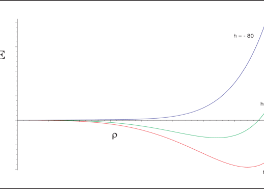
Figure 1: Energy density for the $D$-string with non-trivial world-volume electric field $F_{[2]}$ and background RR 5-form field strength $h$. In the figure we show the potential as a function of the radius $\rho$ for three values of $h$, $F_{\tau\sigma}=\sqrt{2}$ and $\lambda=1$. (See Appendix A for definitions).

In particular, if we fix $F_{\tau\sigma}=\sqrt{2}$ and $\lambda=1$, then the expression for $\rho_{0}$ simplifies giving

$$\rho_{0}=\left({h(2n+3)\over 9\sqrt{2}(c_{2}-1)}\right)^{1/3}.$$ (11)

$CP(2)$ is embedded in $S^{7}$ (see Appendix B). The physical radius of this seven-sphere corresponds in the fuzzy case to

$$R=\lambda\sqrt{Tr(\Phi^{i}\Phi_{i})/N}=\lambda\sqrt{c_{2}}\rho.$$ (12)

Solving for $\rho$ in this example, we get

$$R=\left({h(2n+3)c_{2}^{3/2}\over 9\sqrt{2}(c_{2}-1)}\right)^{1/3}.$$ (13)

that in the large $N$ limit gives

$$R\sim\hbox{${\sqrt{2}h\over 27}$}n^{2/3}.$$ (14)

In the above expression we can see how the radius increases with the number of $D$1-branes and the strength of the RR field. Also, note that in order to achieve this effect we needed a nontrivial electric field on the $D$1-brane, so that we have fundamental strings diluted into the $D$1-brane in our model.

Therefore, we have found new type of solutions corresponding to $N$ $D$1-branes forming a fuzzy $CP(2)$, with an obstruction for topology change. In the large $N$ limit this configuration goes over a $D$5-brane with topology $R^{(1,1)}\times CP(2)$, where $R^{(1,1)}$ comes from the worldsheet expanded by the original $N$ $D$1-branes.

In fact, we can check this correspondence by looking at the different couplings of the non-abelian $D$1-branes to various RR fields. For example, consider the coupling to the RR 6-form potential $C^{[6]}$,

$${\mu_{1}\over 2}\int{{\rm Str}\left(P[\lambda^{2}(i_{\Phi}i_{\Phi})^{2}C^{[6]}]\right)}.$$ (15)

where $P$ is the pull-back from space-time to the world-volumme of the $D$1-brane, and the symbol $i_{\Phi}$ is a non-abelian generalization of the interior product with the coordinates $\Phi^{i}$ (see appendix A for more definitions and notation).

Using the fact that $C^{[6]}$ must have support on the fuzzy $CP(2)$ we write

$$C^{[6]}=C_{\tau\sigma ijkl}\propto C_{\tau\sigma 1\,2\,3\,4}\;d^{pq}_{\;\;\;[i}f_{\;\;jk}^{p}f_{\;\;lm]}^{p}{x^{m}\over r}$$ (16)

where the indices $(1,2,3,4)$ stand for the four real directions on the $CP(2)$ and $\alpha=\hbox{${16\over\sqrt{27}}$}$. Hence the Chern-Simons term (see Appendix A) gives,

$${\mu_{1}\alpha\over 2}\int{d\tau d\sigma{\rm Str}\left(\lambda^{3}C_{\tau\sigma 1\,2\,3\,4}{\Phi^{i}\Phi^{j}\Phi^{k}\Phi^{l}\Phi^{m}\over R}d^{pq}_{\;\;\;[i}f_{\;\;jk}^{p}f_{\;\;lm]}^{p}\right)}.$$ (17)

Therefore, after using the fuzzy solution (8) with $\mu_{1}=4\pi^{2}\mu_{5}\lambda^{2}$ and volume of $CP(2)$ equal to $8\pi^{2}$ we get,

$${\mu_{5}\alpha N(2n+3)\over 16\,c_{2}^{3/2}}\int{d\tau d\sigma\;(8\pi^{2})\;R^{4}C_{\tau\sigma 1\,2\,3\,4}}.$$ (18)

which in the limit of large $N$ takes the form of the coupling of a single $D$5-brane ,

$$\lim_{n\rightarrow\infty}{\alpha N(2n+3)\over 16\,c_{2}^{3/2}}=1.$$ (19)

There exist other types of examples of non-Abelian $D$-branes forming higher dimensional $D$-branes, where the resulting geometry is a fuzzy CP(2) manifold. These cases however, are different in nature from the one presented here since the resulting fuzzy geometry is determined by the lowest energy condition and not by the equations of motion. The dual picture corresponding to $D$-branes with CP(2) topology has already been studied, we refer the reader to [14] for further information.

4 Summary

In this article we have studied the relation between Lie group representations, fuzzy geometries and topology change in matrix models appearing in $M$-theory (i.e non-abelian $D$-branes, Matrix string theory and M(atrix) theory). There are two different types of transitions that lead to the topology change: The first type is related to reducible representations of the Lie group, where a cascade from reducible representations to an irreducible ones does not change the type of the irreducible representation (i.e the type of coset of the Lie group) that appear in the decomposition of the the original representation: i.e these are the transitions of the type $S^{2}\times S^{2}\times\cdots S^{2}\rightarrow S^{2}$. and are due to the difference in energy between these solutions. Recall that reducible representations are direct sums of irreducible representations, where each irreducible representation gives a fuzzy manifold. The second type of topology change is related to a transition between different types of cosets that can be defined in a given Lie group (i.e these are transitions of the type $CP(2)\rightarrow S^{2}$, etc.). Again, these solutions also have different energies which triggers the topology change. Note, however, that these cosets define different fuzzy geometries found within the Lie group.

These topology changing processes are consequences of the fact that the generic equations of motion do not discriminate between representations or cosets of the Lie group. There is a degeneracy between the solutions that translates into topology changing processes.

By introducing higher rank Lie groups and by turning on more background and world-volume fields in the effective $D$-brane action, we were able to find an obstruction to the topology change involving transitions between different cosets (e.g. $S^{2}\rightarrow CP(2),etc.$) corresponding to different types of IRR’s present in the decomposition of the solution. Basically, we found that the corresponding equation of motion determined the irreducible representation of the matrix-valued scalars. This is equivalent to fixing the type of coset of the Lie group, therefore ruling out this type of transition.

These new solutions correspond to $D$1-branes forming $D$5-branes with topology $R^{(1,1)}\times CP(2)$.

Appendix A Non-Abelian $D$-brane action

In the following, we define the conventions used for the $D$-brane action. We borrow almost all of the conventions from Myers [1, 7].

Our starting point is the low energy action for $N$ $D$-strings with non-trivial world-volume electric field $F^{[2]}$. In the background we have a trivial dilaton $\phi$, a flat metric $G$ and zero B-field. For the Ramond sector we include a 4-form potential $C^{[4]}$. The action of the $N$-D1-branes has two separated terms, the Born-Infeld and the Chern-Simon actions. The Born-Infeld action is given by

$$S_{BI}=-T_{1}\int d\tau d\sigma\,{\rm STr}\left(e^{-\phi}\sqrt{-\left(P\left[G_{ab}+G_{ai}(Q^{-1}-\delta)^{ij}G_{jb}\right]+\lambda F_{ab}\right)\,det(Q^{i}{}_{j})}\right),$$ (20)

with

$$Q^{i}{}_{j}\equiv\delta^{i}{}_{j}+i\lambda\,[\Phi^{i},\Phi^{k}]\,G_{kj}\ ,$$ (21)

and the Chern-Simons action is

$$S_{CS}=\mu_{1}\int d\tau d\sigma\;{\rm STr}\left(P\left[e^{i\lambda\,i_{\Phi}i_{\Phi}}(C^{(4)})\right]\,e^{\lambda F}\right)\ ,$$ (22)

where below we explain all the conventions:

• Indices to be pulled-back to the world-volume (see below) have been labelled by $(a,b,..)$. Space-time coordinates are labelled by the indices $(A,B,..)$. The index $(i,j,...)$ labels only directions perpendicular to the $D$1-brane.

• The parameter $\lambda$ is equal to $2\pi l_{s}^{2}$, where $l_{s}$ is the string length scale and $T_{1}$ is the D1-brane tension.

• The center-of-mass degrees of freedom do not decouple, but it will not be relevant for our discussion as we will consider static configurations independent of the space-like world-volume direction. The fields $\Phi^{i}$ thus take values in the adjoint representation of $SU(N)$. As a result, the fields satisfy ${\rm Tr}\,\Phi^{i}=0$ and form a non-abelian generalization of the coordinates specifying the displacement of the branes from the center of mass. These coordinates have been normalized to have dimensions of $(length)^{-1}$ multiplied by $\lambda^{-1}$.

• $P$ stands for the non-abelian “pullback” of various covariant tensors to the world-volume of the $D$1-brane. We will use the static gauge $x^{0}=\tau,x^{1}=\sigma,x^{i}=\lambda\Phi^{i}$ for a coordinate $x$ with origin at the $D$1-brane center-of-mass.

• The symbol $STr$ will be used to denote a trace over the $SU(N)$ indices with a complete symmetrization over the non-abelian objects in each term. The symbol $i_{\Phi}$ is a non-abelian generalization of the interior product with the coordinates $\Phi^{i}$, for example given a 2-form RR potential $C^{[2]}$,

  $$i_{\Phi}\left(\frac{1}{2}C_{AB}dX^{A}dX^{A}\right)=\Phi^{i}C_{iB}dX^{B}.$$ (23)

If we restrict our study to static configurations involving eight nontrivial scalars $\Phi^{i}$, ${i=1,..,8}$, the world-volume field strength $F^{[2]}=F_{\tau\sigma}\;d\tau\wedge d\sigma$ and the the RR field strength $F_{[5]}$, the above action (Born-Infeld plus Chern-Simons) gives the following Lagrangian density:

$$L(\Phi,F^{[2]},F_{[5]})=-\mu_{1}\lambda^{2}\;{\rm STr}\left[{1\over 2}(\partial\Phi)^{2}+{1\over 4}\Phi^{ij}\Phi_{ji}+{1\over 4}F^{2}_{[2]}\right]+$$

$$-\mu_{1}\lambda^{4}\;{\rm STr}\left[{1\over 4}\partial\Phi^{i}\partial\Phi_{i}\Phi^{jk}\Phi_{kj}-{1\over 2}\partial\Phi^{i}\partial\Phi^{j}\Phi_{jk}\Phi^{k}_{\;\;i}-{1\over 8}\Phi^{ij}\Phi_{jk}\Phi^{kl}\Phi_{li}+\right.$$

$$\hskip 56.9055pt\left.+{1\over 16}(\Phi^{ij}\Phi_{ji})^{2}+{1\over 16}F^{2}_{[2]}\Phi^{ij}\Phi_{ji}+{1\over 10}\Phi^{i}\Phi^{j}\Phi^{k}\Phi^{l}\Phi^{m}F_{mlkji}F_{\tau\sigma}\right],$$ (24)

where $\Phi^{ij}\equiv[\Phi^{i},\Phi^{j}]$.

The equation of motion obtained from the variation of $\Phi^{i}$ in (24) gives

$$(1+{1\over 4}\lambda^{2}F^{2})[\Phi^{j},\Phi_{ji}]+{1\over 2}\lambda^{2}[\Phi^{j},\Phi_{ji}(\Phi^{kl}\Phi_{lk})]-{1\over 2}\lambda^{2}[\Phi^{j},(\Phi_{jk}\Phi^{kl}\Phi_{li}-\Phi_{ik}\Phi^{kl}\Phi_{lj})]$$

$$+{1\over 2}\lambda^{2}F_{\tau\sigma}\{\Phi^{jk},\Phi^{lm}\}F_{ijklm}=0.\,\;\;\;\;\;\;$$ (25)

The $U(1)$ part of this equation involves the coupling to the world-volume electric field and can be solved trivially using the ansatz of constant electric field. That leaves only the $SU(N)$ part. Using the ansatze (7) and (8), we then get the equation

$$\left[(1+\hbox{${\lambda^{2}F^{2}\over 4}$})3\rho^{3}+\hbox{${9\over 4}$}(c_{2}-1)\lambda^{2}\rho^{7}\right]T^{i}-\left[\hbox{${3\over 4}$}\lambda^{2}F_{\tau\sigma}h\rho^{4}\right]d^{ijk}T_{j}T_{k}=0,$$ (26)

where $c_{2}$ is the quadratic Casimir operator constructed from $T^{i}$, and we have used the fact that the quartic Casimir operator of $SU(3)$ is proportional to the square of the quadratic Casimir $c_{2}$ [19].

Appendix B Fuzzy Geometry and $CP(n)$

In this appendix we will give a brief description of some of the ideas used in non-commutative geometry that are relevant to this paper and derive all the necessary equations used in the previous chapters. This introduction will be sketchy, since being an active field there are many new papers that appear almost daily. We refer any interested reader to one of the several reviews available in the literature [22, 10, 11, 20].

The field of non-commutative geometry is not new [21]. Recently, it has been given much attention due to the appearance of non-commutative effects in the low energy effective physics of $D$-branes - the very effect we are studying here. However, one does not have to think of non-commutativity as being only the effective description of the theory. Assuming the fundamental structure of space-time to be that of some non-commutative algebra, one can try to derive corresponding consequences for the large-distance (low energy) physics. By its very nature this point of view leads to mixture of the “gravitational” and field theory degrees of freedom. [10, 11, 22].

There is another, more pragmatic reason for introducing non-commutative manifolds into physics. It is the ever-present need for regularization of quantum field theories (QFT’s). The usual, cut-off or lattice regularizations are very successful in many numerical aspects of the problem, but are usually associated with breaking of space-time symmetries of the underlying theory. They produce such unpleasant effects as fermion doubling or loss of general covariance in intermediate computations. However, when introducing the non-commutativity between coordinates, one can at times include the symmetry algebra one seeks to preserve as part of the algebra generated by coordinates. In this case, if the Lagrangian is invariant under the symmetry transformations, the corresponding noncommutative theory will have the symmetry preserved. (The best example is the fuzzy sphere [23, 11]).

Let us now describe one particular procedure of obtaining a non-commutative manifold. We start by promoting the coordinates $\xi_{i}$ of the system to become operators $\hat{\xi}_{i}$ satisfying the non-commutative algebra

$$\xi_{i}\rightarrow\hat{\xi}_{i}\ \ \ \ \left[\hat{\xi}_{i},\hat{\xi}_{j}\right]=C(\hat{\xi})_{ij},$$ (27)

where $C(\xi)_{ij}$ is a skew-symmetric function of $\xi$ (with definite ordering). Then, one looks for all possible matrix representations of this algebra. Each representation is realized by a set of operators acting on a Hilbert space.

At this point we still do not know what ”manifold” we are talking about - the reason being that the very notion of a ”point” has disappeared: there are only matrices now. In general, properties of the manifold can be encoded in the different characteristics of the algebra of functions defined over it. If one wants to know which functions one can get in the commutative limit (i.e. limit when $C(\hat{\xi})_{ij}\rightarrow 0$), it is convenient to introduce the notions of coherent states (CS) and the diagonal coherent state representation [24]. The coherent state of our interest is obtained by acting with the group element $g$ in one particular representation $g\rightarrow T(g)$ on a highest weight vector $|\mu\rangle$ of the Hilbert space associated with the representation:

$$|g\rangle\equiv T(g)|\mu\rangle.$$ (28)

For any operator $\hat{O}$ in the Hilbert space one can compute the so-called symbol of the operator, defined as the diagonal matrix element over the different coherent states:

$$O(g)=\langle g|\hat{O}|g\rangle.$$ (29)

Due to the over-completeness of the generic set of coherent states, the symbol (B.3) of the operator contains information about any matrix element of this operator and determines the operator. These symbols give the functions $O$ on the manifold. Suppose that a highest weight vector of some representation transforms by a singlet representation of a subgroup $H$ of $G$:

$$H\subset G,\ \ \ \forall h\in H:\ \ T(h)|\mu\rangle=e^{i\alpha(h)}|\mu\rangle.$$ (30)

So $|\mu\rangle$ changes only by a phase $e^{i\alpha(h)}$ ($\alpha(h)$ is real). Due to this feature one can see that

$$O(g) = \langle g|\hat{O}|g\rangle=\langle\mu|T^{\dagger}(g)|\hat{O}|T(g)|\mu\rangle=\langle\mu|T^{\dagger}(h)T^{\dagger}(g)|\hat{O}|T(g)T(h)|\mu\rangle=$$ (31)

$$= \langle\mu|T^{\dagger}(gh)|\hat{O}|T(gh)|\mu\rangle\Leftrightarrow O(g)=O(gh),\ \ \ \forall h\in H.$$

This invariance property means that the functions on $G$ that one gets this way are identical to functions on the coset $G/H$. This shows that the non-commutative manifold is defined not only by the right hand side of (27), but also by the representation chosen.

After doing all of the above, one can construct the “field theory” on this manifold. Values of the fields become matrices and all the integrals over volume become traces in this Hilbert space $\cal H$: $\int V(\Phi)\rightarrow{\rm Tr}_{\cal H}(V(\hat{\Phi}))$. A priori, the dimension of this Hilbert space (representation) can be infinite, i.e. traces can include infinite summations. Thus from the point of view of regularization, the main goal is to obtain suitable manifolds associated with finite-dimensional Hilbert spaces. Generally this cannot be done, but there is a class of manifolds for which this is virtually guaranteed - these are the co-adjoint orbits of compact Lie groups [25]. This means that the right hand side of (27) should be $C(\hat{\xi})_{ij}=i\,f_{ijk}\,\hat{\xi}_{k}$, where $f_{ijk}$ is the appropriate (e.g. $SU(N)$) structure constants.

Let us now give several examples which have been studied in the literature using some of the ideas described above:

• ”Moyal plane”. In this case one has only two dimensions $x_{1},x_{2}$, and $C_{ij}$ is just $\epsilon_{ij}$. This is the well-known harmonic oscillator ($h.o.$) algebra and the Hilbert space is the infinite-dimensional set spanned by linear combinations of of $h.o.$ excited states, $|n\rangle$.

• The ”fuzzy” sphere $S^{2}=CP(1)$. It is the coset $SU(2)/U(1)$ and is the orbit of say the $\sigma_{3}$ generator under the adjoint action of $SU(2)$. The corresponding algebra is just the usual angular momentum one, with $C_{ij}=i\,\epsilon_{ijk}\xi_{k}$. All the irreducible representations (IRR’s) can be obtained from symmetric products of the fundamental representation and can be labelled by $j\in Z^{+}/2$. All the fields become $(2j+1)\times(2j+1)$ matrices and all the traces become finite (there are only $2j+1$ terms in each sum.) One can then put field theory on this fuzzy manifold and obtain, for example, an explicit expression for the path integral which is finite dimensional [26, 11]. It is quite interesting that upon introducing fermions in the model, there are also arguments why this construction avoids the famous fermion doubling problem (see [12], the first three papers of [23] and [11]).

• $CP(2)=SU(3)/U(2)$. This coset is the $SU(3)$ orbit of the “hypercharge”:$Y=diag(1,1,-2)$ under the adjoint action. The corresponding representations are totally symmetric products of $3$’s or $3^{*}$’s. The corresponding Hilbert space has dimension $(n+1)(n+2)/2$ for any positive integer $n$. This manifold has been obtained as one of the solutions in [14, 27] and analyzed in [28, 18].

• $SU(3)/(U(1)\times U(1))$. This is the ”other” coset of the $SU(3)$ which was obtained as one of the possible solutions in [14]. It is the orbit of the (1,-1,0) generator of $SU(3)$ under the adjoint action and produces representations which have zero hypercharge.

For the purposes of this paper, we need one of the $CP(n)$ type manifolds, namely $CP(2)$. It has been extensively studied in [28, 18]. Here we will present only the relevant facts along the lines of Alexanian et al. [18].

The classical, ”continuous” $CP(2)$ manifold can be obtained as one particular coset of $SU(3)$: $CP(2)=SU(3)/U(2)$ (this is general: $CP(n)=SU(n+1)/U(n)$). What is important for us is that $CP(2)$ is the adjoint orbit of the hypercharge in $SU(3)$, i.e.

$$t^{a}\,\xi^{a}={\rm constant}\times U\,t^{8}\,U^{-1},\ \ \ \ U\in SU(3),\ \ a=1,2,...8,$$ (32)

repeated indices being summed over. Here $t^{a}$’s are generators of $SU(3)$ in the fundamental representation (where $t^{a}=\lambda^{a}/2$, $\lambda$’s being the Gell-Mann matrices). In this formula $\xi^{a}$ are coordinates in $R^{8}$ and $U$ is an arbitrary $SU(3)$ matrix. This equation defines $CP(2)$ as a surface in $R^{8}$. With the constant=1 for simplicity, squaring both sides of (32) and tracing, we also get

$$\xi^{i}\,\xi^{i}=2\,{\rm tr}(U\,t^{8}\,U^{-1}\,U\,t^{8}\,U^{-1})=2\,{\rm tr}(t^{8}\,t^{8})=1.$$ (33)

Therefore $CP(2)\subset S^{7}$.

Using the property of $t^{8}$ (or hypercharge) that

$$(t^{8})^{2}=\frac{1}{6}-\frac{1}{2\sqrt{3}}t^{8},$$ (34)

one can show that the $\xi$’s so defined also satisfy

$$\xi^{a}\,=\,{\rm constant}\times d^{abc}\,\xi^{b}\,\xi^{c},$$ (35)

where $d^{abc}$ is the standard totally symmetric traceless invariant $SU(3)$ tensor. The remarkable fact is that this statement can be reversed, i.e.

$$\xi^{a}\,=\,{\rm constant}\times d^{abc}\,\xi^{b}\,\xi^{c}\ \ \Rightarrow\ \ \xi\in CP(2),$$ (36)

so that this equation can be used to define $CP(2)$ [18].

In the non-commutative case, the coordinates $\xi^{i}$ will become operators $\hat{\xi}^{i}$ in an appropriate Hilbert space which satisfy $SU(3)$ commutation relations. Naively, one may try to use any irreducible representation of $SU(3)$ to represent the $\xi$’s. However, only the totally symmetric ones produce $CP(2)$ in the commutative limit [18]. This is because only the symmetric representations have highest weight vectors with the $U(2)$ stability group, which, according to the discussion above leads to the $SU(3)/U(2)=CP(2)$ coset in the continuous limit.

We will show now that the imposition of the condition (36) as an operator equation

$$\hat{\xi}^{a}\,=\,{\rm constant}\times d^{abc}\,\hat{\xi}^{b}\,\hat{\xi}^{c},\ \$$ (37)

allows only totally symmetric representations of $SU(3)$. First we note that any irreducible representation of the group $SU(3)$ can be obtained from the direct product of the totally symmetric product of fundamental (with generators $t_{i}$) and the totally symmetric product of anti-fundamental(with generators $-{t^{*}}_{i}$) representations. Assuming for the moment that the fundamental representation satisfies (37) for some value of the “constant”, we can immediately see that by replacing $t_{i}\rightarrow-t^{*}_{i}$, the “constant” will have to change sign as well. Therefore, any representation that has both fundamental and anti-fundamental components present in its decomposition cannot satisfy this equation with ${\rm constant}\,\neq\,0$. This means that only totally symmetric products of the fundamental (or anti-fundamental) representations are allowed.

This is exactly what we have to use in the text to obtain $CP(2)$ as a solution of the equations of motion, and not a choice of the energy condition.

In order to do an explicit calculation one can use the Schwinger representation for the generators $\hat{\xi}^{a}$. Using three harmonic oscillators with annihilation and creation operators $a_{i},a_{i}^{+},\ i=1,2,3$ where $[a_{i},a^{+}_{j}]=\delta_{ij}$, one has $\hat{\xi}^{a}=\alpha\,a^{+}_{i}(t^{a})_{ij}a_{j}$, where $\alpha$ is some constant to be determined later. $\hat{\xi}^{a}$ acts on the Fock space with basis $\prod(a^{+}_{i})^{n_{i}}|0\rangle=|n_{1},n_{2},n_{3}\rangle$ which are symmetric under interchange of $a^{+}_{i}$’s. As $[\hat{\xi}^{a},a^{+}_{j}]=\alpha\,a^{+}_{j}(t^{a})_{ji}$, we thus get only symmetric products of the fundamental representation. For a similar construction for anti-fundamental representation, we must start from $\hat{\xi}^{a}=-\beta\,b^{+}_{i}{(t^{a})}^{*}_{ij}b_{j}$, where $b_{i},b^{+}_{j}$ are also bosonic oscillators (commuting with $a_{k},a^{+}_{k}$) and $\beta$ is a constant. Now the operators $\sim a^{+}\,t^{a}\,a$ act irreducibly on the subspace spanned by $|n_{1},n_{2},n_{3}\rangle$, with $n_{1}+n_{2}+n_{3}=n$ held fixed, $n$ being an arbitrary positive integer. The dimension $N$ of this Hilbert space is easily obtained as $N=(n+1)(n+2)/2$. After a straightforward but somewhat tedious computation, (see [18] for details), one then gets,

$$d_{abc}\hat{\xi}_{a}\hat{\xi}_{b}=2t^{a}_{\alpha\beta}\left(\frac{n}{6}+\frac{1}{4}\right)a^{\dagger}_{\alpha}a_{\beta}=\frac{\left(\frac{n}{3}+\frac{1}{2}\right)}{\sqrt{\frac{1}{3}n^{2}+n}}\hat{\xi}_{a}.$$ (38)

Let us choose the value of $\alpha$ so that $\sum_{i}\hat{\xi}_{i}\hat{\xi}_{i}=I$, the identity operator. Using the value $\frac{1}{3}n^{2}+n$ of the the quadratic Casimir in the symmetric representation $c_{2}$ one can see that $\alpha=1/c_{2}^{1/2}$, so $\alpha=1/\sqrt{n^{2}/3+n}$.

References

- [1] R.C. Myers, JHEP 9912 (1999) 022, hep-th/9910053.
- [2] W. Taylor, M. Van Raamsdonk, Nucl.Phys. B558 (1999) 63-95 and hep-th/9904095; Nucl.Phys. B573 (2000) 703-734 and hep-th/9910052.
- [3] T. Banks, W. Fischler, S.H. Shenker and L. Susskind, Phys.Rev. D55 (1997) 5112-5128 and hep-th/9610043; L. Susskind, hep-th/9704080.
- [4] R. Dijkgraaf, E. Verlinde, H. Verlinde, Nucl.Phys. B500 (1997) 43-61 and hep-th/9703030.
- [5] T. Banks and N. Seiberg, Nucl.Phys. B497 (1997) 41-55 and hep-th/9702187; R. Dijkgraaf, E. Verlinde and H. Verlinde, Nucl.Phys.Proc.Suppl. 62 (1998) 348-362 and hep-th/9709107; Lubos Motl, hep-th/9701025.
- [6] R. Schiappa, Nucl.Phys. B608 (2001) 3-50 and hep-th/0005145.
- [7] P. J. Silva, JHEP 0202 (2002) 004 and hep-th/0111121.
- [8] C. B. Thorn, Phys.Rev. D56 (1997) 6619 and hep-th/9707048. O. Bergman and C. B. Thorn, Phys.Rev. D52 (1995) 5980-5996 and hep-th/9506125
- [9] P. Townsend, PASCOS/Hopkins 1995:0271-286 and hep-th/9507048.
- [10] J. Madore, An Introduction to Noncommutative Differential Geometry and its Physical Applications, Cambridge University Press, 330p. 2nd ed., Cambridge (1999).
- [11] A.P. Balachandran, “Quantum spacetimes in the year 2002”, Pramana 59 359 (2002) and hep-th/0203259; “video conference” course on “Fuzzy Physics” at http://www.phy.syr.edu/courses/FuzzyPhysics/ and http://bach.if.usp.br/ teotonio/FUZZY/.
- [12] H. Grosse and P. Prešnajder, Lett.Math.Phys. 33, 171 (1995) and references therein; H. Grosse, C. Klimčík and P. Prešnajder, Commun.Math.Phys. 178,507 (1996); 185, 155 (1997); H. Grosse and P. Prešnajder, Lett.Math.Phys. 46, 61 (1998) and ESI preprint, 1999; H. Grosse, C. Klimčík, and P. Prešnajder, Commun.Math.Phys. 180, 429 (1996) and hep-th/9602115; H. Grosse, C. Klimčík, and P. Prešnajder, in Les Houches Summer School on Theoretical Physics, 1995, hep-th/9603071; P. Prešnajder, J.Math.Phys. 41 (2000) 2789-2804 and hep-th/9912050; J. Madore gr-qc/9906059.
- [13] J. Castelino, S. Lee and W. Taylor, Nucl.Phys. B526 (1998) 334-350 and hep-th/9712105.
- [14] S. P. Trivedi and S. Vaidya, JHEP 0009 (2000) 041 and hep-th/0007011.
- [15] N. R. Constable, R. C. Myers and O. Tafjord, JHEP 0106 (2001) 023 and hep-th/0102080.
- [16] P. Ming Ho and S Ramgoolam, Nucl.Phys. B627 (2002) 266-288 and hep-th/0111278.
- [17] D. P. Jatkar, G. Mandal, S. R. Wadia and K.P. Yogendran, JHEP 0201 (2002) 039 and hep-th/0110172. K. Hashimoto, hep-th/0204203. J. Madore and L.A. Saeger, Class.Quant.Grav. 15 (1998) 811-826 and gr-qc/9708053.
- [18] G.Alexanian, A.P.Balachandran, G.Immirzi and B.Ydri, J.Geom.Phys. 42 (2002) 28-53 and hep-th/0103023.
- [19] S. Okubo, J. Math. Phys. 20, 586 (1979).
- [20] M. R. Douglas and N. A. Nekrasov, “Noncommutative field theory,” Rev. Mod. Phys. 73, 977 (2002) and hep-th/0106048; A. Connes, “Noncommutative geometry: Year 2000,” math.qa/0011193;
- [21] H. S. Snyder, “Quantized Space-Time,” Phys. Rev. 71, 38 (1947).
- [22] A. Connes, Noncommutative Geometry, Academic Press, London, 1994; G. Landi, An Introduction to Noncommutative Spaces And Their Geometries, Springer-Verlag, Berlin, 1997 and hep-th/9701078; J. M. Gracia-Bondia, J. C. Varilly and H. Figueroa, Elements Of Noncommutative Geometry, Boston, USA: Birkhauser (2001) 685 p.
- [23] A.P. Balachandran and S. Vaidya, Int.J.Mod.Phys. A16, 17 (2001) and hep-th/9910129; A. P. Balachandran, T. R. Govindarajan and B. Ydri, hep-th/9911087; A. P. Balachandran, T. R. Govindarajan and B. Ydri, Mod.Phys.Lett. A15, 1279 (2000) and hep-th/0006216; A. P. Balachandran, X. Martin and D. O’Connor, Int.J.Mod.Phys. A16, 2577 (2001) and hep-th/0007030; S. Vaidya, Phys. Lett. B512 403 (2001) and hep-th/0102212.
- [24] J.R. Klauder and B.-S. Skagerstam, Coherent States: Applications in Physics and Mathematical Physics, World Scientific (1985); A.M. Perelomov: Generalized Coherent States and their Applications, Springer-Verlag, (1986); M. Bordemann, M. Brischle, C. Emmrich and S. Waldmann, J. Math. Phys. 37, 6311 (1996); M. Bordemann, M. Brischle, C. Emmrich and S. Waldmann, Lett. Math. Phys. 36, 357 (1996); S. Waldmann, Lett. Math. Phys. 44, 331 (1998); G. Alexanian, A. Pinzul and A. Stern Nucl. Phys. B600 531 (2001) and hep-th/0010187; A.P. Balachandran, B.P. Dolan, J. Lee, X. Martin and D. O’Connor, J.Geom.Phys. 43, 184 (2002) and hep-th/0107099.
- [25] A.A. Kirillov, Encyclopedia of Mathematical Sciences, vol 4, p.230; B. Kostant, Lecture Notes in Mathematics, vol.170, Springer-Verlag (1970), p.87.
- [26] H. Grosse, C. Klimcik and P. Presnajder, Int. J. Theor. Phys. 35, 231 (1996) and hep-th/9505175.
- [27] V. P. Nair and S. Randjbar-Daemi, Nucl. Phys. B533, 333 (1998) and hep-th/9802187.
- [28] H.Grosse and A.Strohmaier, Lett.Math.Phys. 48,163(1999) and hep-th/9902138.