Quiver Theories, Soliton Spectra and Picard-Lefschetz transformations

Abstract:

Quiver theories arising on D3-branes at orbifold and del Pezzo singularities are studied using mirror symmetry. We show that the quivers for the orbifold theories are given by the soliton spectrum of massive $2d$ ${\cal N}$=2 theory with weighted projective spaces as target. For the theories obtained from the del Pezzo singularities we show that the geometry of the mirror manifold gives quiver theories related to each other by Picard-Lefschetz transformations, a subset of which are simple Seiberg duals. We also address how one indeed derives Seiberg duality on the matter content from such geometrical transitions and how one could go beyond and obtain certain “fractional Seiberg duals.” Moreover, from the mirror geometry for the del Pezzos arise certain Diophantine equations which classify all quivers related by Picard-Lefschetz. Some of these Diophantine equations can also be obtained from the classification results of Cecotti-Vafa for the $2d$ ${\cal N}=2$ theories.

1 Introduction

The technology of D3-branes probing singularities as a method of establishing classes of gauge theories in four dimensions is by now a well-establish subject. Indeed we are interested in local algebraic models of non-compact Calabi-Yau threefolds that give ${\cal N}=1$ supersymmetric gauge theories. In addition to the orbifolds pioneered by Douglas-Moore and followups [1], toric singularities have also been extensively investigated [2, 3, 4, 5].

Attention has been paid of late to del Pezzo surfaces [6, 4, 7, 8]. Indeed with the rôle of mirror symmetry [9, 10] in the geometrisation of ${\cal N}=1$ dualities [11, 12, 13, 14, 15], D3-branes probing the cone over del Pezzo surfaces as well as the mirror perspective of D6-branes wrapping special Lagrangian three-cycles have been increasingly important. An intriguing matter has been the realisation of Seiberg’s duality in terms of what has been called “Toric Duality” [4, 5, 16, 17, 18].

Treading upon this path, the quiver theories we are interested in are ${\cal N}=1$, supersymmetric $D=4$ gauge theories arising on the worldvolume of D3-branes transverse to a Calabi-Yau threefold with del Pezzo singularity in the Type IIB background. If the singularity is not an orbifold singularity it is difficult to obtain the information about the gauge groups and the matter content. However, it was shown in [8] that mirror symmetry provides a powerful tool in determining the gauge groups and the quiver diagrams representing the matter. In [13] mirror symmetry was used to engineer Seiberg dual theories arising on the toric del Pezzo singularities and a conjecture was given for calculating the superpotential. It was shown that under certain Picard-Lefshetz transformation the superpotential transforms as expected from Seiberg duality. Also in the case of $\mathbb{P}^{1}\times\mathbb{P}^{1}$ a duality cascade was engineered using the results of [10].

In this paper we continue to study the gauge theories arising on the D3-branes from the mirror symmetry perspective as D6-branes wrapped on 3-cycles in Type IIA. We study the case of del Pezzos in more detail by giving an exceptional collection forming a helix on the del Pezzo surface and show that this exceptional collection gives the correct Ramond charges for the massive theory with del Pezzo surfaces as the target space. The exceptional collections also give the charges of the fractional branes in the Type IIB description and therefore the constraint that we get correct Ramond charges from a collection of bundles on the del Pezzo surfaces gives us certain Diophantine equations which classifies all quiver gauge theories related to each other by Picard-Lefschetz transformations. We also obtain the same Diophantine equations from the geometry of the Calabi-Yau mirror to the local del Pezzos.

Besides del Pezzos, orbifold singularities provide an interesting class of singularities of the Calabi-Yau threefolds. These orbifold singularities arise when a four cycle which is a weighted projective space collapses. However, if we resolve the singularities of the weighted projective space as well then the singularity is produced by multiple four cycles collapsing. Mirror symmetry is a powerful tool for studying the gauge theories obtained from these singularities and gives a geometric interpretation to Seiberg duality [13, 15].

Under mirror symmetry D3-branes transverse to a non-compact Calabi-Yau threefold $X$ become D6-branes wrapped on a $T^{3}$ in the mirror Calabi-Yau $Y$ [19, 8, 13]. The homology class of this $T^{3}$ is given by

$$[T^{3}]=\sum_{a=1}^{K}n_{a}S_{a}\,,\,\,n_{a}\in\mathbb{Z}\,,$$ (1)

where $\{S_{1},\cdots,S_{K}\}$, which form a basis of $H_{3}(Y,\mathbb{Z})$, are three cycles topologically equivalent to $S^{3}$ and $n_{a}$ is the wrapping number of cycle $S_{a}$. The D6-brane wrapped on $T^{3}$ gives rise to a ${\cal N}=1$ $D=4$ theory with gauge group $G$ and quiver matrix $Q$ given by [8, 13]

$$G=\prod_{a=1}^{K}U(n_{a})\,,\,\,\,Q_{ab}=S_{a}\cdot S_{b}\,.$$ (2)

In the above equations we have assumed $n_{a}\geq 0$ which can always be arranged by changing the orientation of the 3-cycles $S_{a}$. The quiver matrix is just the intersection matrix of the 3-cycles. In terms of the fractional branes $\{{\cal F}_{1},\cdots,{\cal F}_{K}\}$ (which are mirror to $S_{a}$) on $X$, on Type IIB side, this is given by [7, 20, 8, 13]

$$Q_{ab}=\int_{X}\mbox{ch}({\cal F}_{a}\otimes{\cal F}_{b}^{*})\mbox{Td}(X)\,.$$ (3)

The anomaly cancellation condition is given by

$$0=\sum_{b=1}^{K}n_{b}Q_{ab}=\sum_{b=1}^{K}S_{a}\cdot n_{b}S_{b}=S_{a}\cdot[T^{3}]\,,\,\forall a\,.$$ (4)

and the fact that it is satisfied automatically follows from the geometry of the mirror manifold [8]. Equation (1) gives us a particular solution to the anomaly cancellation condition, more general solutions $\{n_{1},\cdots,n_{K}\}$ can also be found such that $\sum_{i=1}^{K}n_{i}S_{i}$ is not topologically a $T^{3}$, but still has $zero$ intersections with all $S_{a}$.

We can rephrase Equations (3) and (4) in the language of exceptional collections of vector bundles (or sheaves) over the compact divisor of the Calabi-Yau $X$. (q.v.  [9, 10, 8, 13]). Given an exceptional collection

$$\{F_{1},\cdots,F_{K}\}$$ (5)

such that

$$\sum_{a=1}^{K}n_{a}\mbox{ch}_{0}(F_{a})=0,\,\,\sum_{a=1}^{K}n_{a}\mbox{ch}_{1}(F_{a})=0,\,\,\sum_{a=1}^{K}n_{a}\mbox{ch}_{2}(F_{a})=-1,\,\,$$ (6)

we get an anomaly free gauge theory with gauge group and quiver given by

$$G=\prod_{a=1}^{K}U(n_{a})\,,\,\,\,Q_{ab}=\chi(F_{a},F_{b})-\chi(F_{a},F_{b}),$$ (7)

where $\chi(F_{i},F_{j}):=\sum_{m}(-1)^{m}\dim_{\mathbb{C}}{\rm Ext}^{m}(F_{i},F_{j})$. For each subset of the exceptional collection $\{F_{\alpha_{1}},\cdots F_{\alpha_{n}}\}$ there is a term in the superpotential [13](the bi-fundamental fields are $X^{i}_{\alpha\beta}\in\mbox{Hom}(F_{\alpha}\otimes F_{\beta}^{*})$):

$$a_{i_{1}i_{2}\cdots i_{n}}X^{i_{1}}_{\alpha_{1}\alpha_{2}}\cdots X^{i_{n-1}}_{\alpha_{n-1}\alpha_{n}}X^{*\,i_{n}}_{\alpha_{1}\alpha_{n}},$$ (8)

where $X^{*\,i_{n}}_{\alpha_{1}\,\alpha_{n}}\in\mbox{Hom}(F_{\alpha_{1}}\otimes F^{*}_{\alpha_{n}})$ and $a_{i_{1}i_{2}\cdots i_{n}}$ are such that if $f^{i}_{\beta\alpha}:F_{\alpha}\mapsto F_{\beta}$ then

$$f^{i_{n-1}}_{\alpha_{n}\alpha_{n-1}}\cdots f^{i_{2}}_{\alpha_{3}\alpha_{2}}f^{i_{1}}_{\alpha_{2}\alpha_{1}}=a_{i_{1}i_{2}\cdots i_{n-1}i_{n}}f^{i_{n}}_{\alpha_{n}\alpha_{1}}\,.$$ (9)

In other words the terms of the superpotential come from non-zero loop contractions in the quiver, where by contraction we mean composition of maps.

Since $\{F_{1},\cdots F_{K}\}$ is an exceptional collection then we can consider the left and the right mutations [13], with respect to the $l$-th node,

$$\{F_{l},F_{l+1}\} \mapsto \{R_{l}F_{l+1},F_{l}\}\,,$$

$$\mapsto \{F_{l+1},L_{l+1}F_{l}\}\,,$$

dictated by

$$\mbox{ch}(R_{l}F_{l+1})=\mbox{ch}(F_{l+1})-\chi(F_{l},F_{l+1})\mbox{ch}(F_{l})\,,$$ (11)

$$\mbox{ch}(L_{l+1}F_{l})=\mbox{ch}(F_{l})-\chi(F_{l},F_{l+1})\mbox{ch}(F_{l+1})\,.$$

Then, defining $\chi_{l}:=\chi(F_{l},F_{l+1})$, the changes on the gauge group factors and the quiver diagram are:

$$\prod_{a}U(n_{a}) \mapsto \prod_{a=1}^{l-1}U(n_{a})\,\,U(n_{l+1})U(n_{l}+\chi_{l}n_{l+1})\prod_{a=l+2}^{N}U(n_{a})\,,$$

$$\mapsto \prod_{a=1}^{l-1}U(n_{a})\,\,U(n_{l+1}+\chi_{l}n_{l})U(n_{l})\prod_{a=l+2}^{N}U(n_{a})\,,$$

where it is easy to check that these new $n_{a}$ satisfy anomaly free conditions (6). and

$$Q_{ab} \mapsto Q_{ab}\,,\,\,a,b\neq l,l+1\,,$$ (14)

$$Q_{a,l} \mapsto Q_{a,l+1}-\chi_{l}Q_{a,l}\,$$

$$\mapsto Q_{a,l+1}\,,$$

$$Q_{a,l+1} \mapsto Q_{a,l}\,,$$

$$\mapsto Q_{a,l}-\chi_{l}Q_{a,l+1}\,,$$

$$Q_{l,l+1} \mapsto -Q_{l,l+1}\,,$$

$$\mapsto -Q_{l,l+1}\,.$$

Notice that if $n_{l}+\chi_{l}n_{l+1}<0$, we should choose the negative $R_{l}F_{l+1}$ as well as the $Q_{a,l+1}$ calculated above. These mutations are also called Picard-Lefschetz transformations, which we will discuss in detail in Section 5. The field theory interpretation of these mutations is nothing but a realization of Seiberg duality as will be discussed throughout this paper.

The paper is organized as follows. In Section 2 we briefly review the classification of ${\cal N}=(2,2)$ theories, in particular how one could obtain the quiver diagram of ${\cal N}=1$ probes on cones over del Pezzo as the soliton spectrum of these massive theories in 2-dimensions. Subsequently, we show how this technique may be extended to the Abelian orbifold $\mathbb{C}^{3}/\mathbb{Z}_{N}$ in Section 3. We show how we can use exceptional collections over weighted projective spaces, as opposed to $\mathbb{P}^{2}$ and its blowups in the del Pezzo case, to study the quiver theories. Explicit examples are constructed for $\mathbb{C}^{3}/\mathbb{Z}_{5}$. Then in Section 4, we return to the case of the del Pezzos and study in detail how we could wrap D6-branes on the mirror to obtain classes of gauge theories related by Picard-Lefschetz monodromy. Therefrom arise certain Diophantine equations which completely classifies these theories.

We continue in this vein in Section 5 where we show in detail how one derives Seiberg duality rules for the matter content from Picard-Lefschetz, characterized by “$(p,q)$ 7-brane” moves and how one can go beyond and obtain “fractional Seiberg duality.” In Section 6 we briefly remark certain relations between the superpotentials obtained in this setup and the global isometries of the background geometry and also comment on the case of $\mathbb{P}^{2}$, the zeroth del Pezzo, especially its Diophantine equation, in some detail. We end with Conclusions and Prospects in Section 7.

2 Classification of ${\cal N}=(2,2)$ two dimensional theories and solitons

In this section we collect few facts from the theory of massive ${\cal N}=(2,2)$ two dimensional theories and prepare their use for quiver theories. We will see that the quiver diagram for the four dimensional theories we are interested in are identified with the soliton diagram of the massive two dimensional theory.

For a non-homogeneous superpotential $W$ of a massive LG theory, the soliton spectrum is determined by the intersection number of middle dimensional cycles in the geometry defined by

$$W(x,y)=z\,.$$ (15)

The middle dimensional cycles which start at the critical points of the superpotential and project to straight lines in the z-plane are the D-branes of the massive theory [10]. The intersection number of these middle dimensional cycles calculates the Witten index in a sector in which strings are stretched between the two D-branes given by the cycles.

In [10] it was shown that the intersection numbers of three cycles in the mirror CY manifold, $Y$, give the soliton numbers of the massive two dimensional theory with toric del Pezzo as the target space. We will see that the geometry of the mirror CY $Y$ is completely captured by the four dimensional non-compact surface defined by Equation (15) for an appropriate $W$ and therefore the quiver diagram, which is obtained from the intersection number of three cycles, is identified with the soliton diagram of the corresponding massive theory.

From the classification results of [21] we know that an arbitrary soliton diagram does not necessarily correspond to a massive theory as the soliton spectrum is related to the Ramond charges. Let $A$ be an upper triangular matrix such that

$$A_{ab} = 0\,,a\leq b\,,$$ (16)

$$A_{ab} = \mu_{ab}\,,a>b\,,$$

where $\mu_{ab}$ is the number of solitons between the $a$-th and the $b$-th vacua. The eigenvalues $\lambda_{a}$ of the matrix

$$H=(1-A)(1-A)^{-T}\,,$$ (17)

are given by

$$\lambda_{a}=e^{2\pi iq^{R}_{a}}\,$$ (18)

and thus are all phases. This follows from the fact that the matrix $H$ is the monodromy matrix of the D-branes of the massive theory as the massive superpotential $W$ goes to $e^{2\pi i}W$. A derivation of this result is given in Section 4 of [10]. The integer part of the Ramond charge $q^{R}_{a}$ can also be calculated as discussed in [21]. The fact that the eigenvalues must be phases implies that the characteristic polynomial of the matrix $H$

$$P(z)=\mbox{det}(z-H)$$ (19)

is a product of cyclotomic polynomials.

In the case that the target space is a compact Kähler manifold of complex dimension $n$ which satisfies the condition on the Hodge numbers $h^{p,q}=h^{p,p}\delta_{p,q}$, the Ramond charges are given by $p-\frac{n}{2}$, each with multiplicity $h^{p,p}$. Specializing to the case $n=2$, we find that for all del Pezzo surfaces $\mathbb{B}_{k=0,\ldots,8}$ (with $h^{0,0}=h^{2,2}=1,h^{1,1}=k+1)$ the eigenvalues are equal to one, since the charges are integral, and thus the characteristic polynomial is

$$P_{k}(z)=(z-1)^{k+3}\,,\,\,{\rm for}\,\,\mathbb{B}_{k}\,,$$ (20)

where $k+3=\sum_{p}h^{p,p}(\mathbb{B}_{k})=\chi(\mathbb{B}_{k})$.

As an example consider the case of $\mathbb{B}_{3}$. The quivers for this case are given in [4, 5, 8, 17, 16] and all of them are related to each other by Picard-Lefschetz transformation of three cycles. Consider case (IV) of [17] (also case (IV) of [16]):

$$A^{IV}=\begin{pmatrix}0&0&0&0&0&0\\ 0&0&0&0&0&0\\ 0&0&0&0&0&0\\ 1&1&1&0&0&0\\ 1&1&1&0&0&0\\ -2&-2&-2&3&3&0\\ \end{pmatrix}\,,$$ (21)

the characteristic polynomial is given by

$$P(z)=\mbox{det}(z-H)=(z-1)^{6}\,.$$ (22)

By comparing the coefficient of $z^{k+2}$ in Equation (20) we find a necessary condition for the intersection numbers $\mu_{ab}$: the trace of $H$ should be equal to the Euler characteristic of the del Pezzo surface,

$$\mbox{Tr}H=k+3\,.$$ (23)

This gives us a Diophantine equation satisfied by the soliton spectrum of the del Pezzo surfaces. This equation will turn out to play an important role in the study of Seiberg dualities for the given singularity.

We can use this formalism to calculate charges of fractional branes. This is demonstrated in the following two examples:

Example one: Consider the case of $\mathbb{B}_{4}$ ($\mathbb{P}^{2}$ blownup at four points). The basis of $H_{2}(\mathbb{B}_{k})$ we will consider is given by $\{H,E_{1},\cdots,E_{k}\}$ with

$$H\cdot H=1\,,\,E_{a}\cdot E_{b}=-\delta_{ab}\,,\,\,H\cdot E_{a}=0\,.$$ (24)

The following collection of bundles and sheaves is an exceptional collection forming a helix on $\mathbb{B}_{4}$ [10, 7]

$$\{-{\cal O}(-H+E_{1}+E_{2}),{\cal O}_{E_{2}}(0),{\cal O}_{E_{1}}(0),{\cal O}(E_{3}),{\cal O}(-H+E_{3}),$$ (25)

$$\qquad-{\cal O}_{E_{4}}(-1),-{\cal O}(-E_{4})\}$$

Following [10] we define

$$S_{ab}=\int_{\mathbb{B}_{4}}\mbox{ch}(F_{a}\otimes F_{b}^{*})\mbox{Td}(\mathbb{B}_{4})\,.$$ (26)

It is easy to see that the characteristic polynomial of $H=S^{-T}S$ is given by

$$P(z):=\mbox{det}(z-H)=(z-1)^{7}=(z-1)^{\chi(\mathbb{B}_{4})}\,.$$ (27)

Thus the Ramond charges are integers and are given by [21],

$$q_{R}=\{-1,0,0,0,0,0,1\}=\{\frac{p+q-2}{2}~{}|~{}p+q=\mbox{deg}\,\omega_{i},\,\omega_{i}\in H^{p,q}(\mathbb{B}_{4})\}\,.$$ (28)

Where $\omega_{i}$ form a basis of $H^{p,q}(\mathbb{B}_{4})$.

Example two: As another example we consider the case of $\mathbb{B}_{8}$. In this case we consider the following exceptional collection [7],

$$\{{\cal O}(-H+E_{1}+E_{2}+E_{7}),{\cal O}_{E_{7}},{\cal O}_{E_{2}},{\cal O}_{E_{1}},{\cal O}_{H-E_{3}-E_{6}},{\cal O}(-H+E_{6}),$$

$$\qquad{\cal O}(-E_{5}),-{\cal O}_{H-E_{3}-E_{5}}(1),-{\cal O}_{E_{4}}(-1),-{\cal O}_{E_{8}}(-1),-{\cal O}(-E_{4}-E_{8})\}\,.$$

The characteristic polynomial of $H=S^{-T}S$, where $S$ is defined as before, is

$$P(z) = (z-1)^{11}=(z-1)^{\chi(\mathbb{B}_{8})}\,.$$ (29)

And the Ramond charges are given by ($p+q=\mbox{deg}H^{p,q}(\mathbb{B}_{8})$)

$$q_{R} = \{-1,0,0,0,0,0,0,0,0,0,1\}=\{\frac{p+q-2}{2}\,|\,p+q=\mbox{deg}\,\omega_{i},\,\omega_{i}\in H^{p,q}(\mathbb{B}_{8})\}\,.$$ (30)

Where $\omega_{i}$ form a basis of $H^{p,q}(\mathbb{B}_{8})$.

As discussed in detail in [10] these exceptional collections are not unique and other exceptional collections can be obtained by mutations. However, all exceptional collections must give same Ramond charges and therefore Equation (23) must be satisfied. This gives a severe constraint on the integers $S_{ab}$. In the case of $\mathbb{B}_{0}:=\mathbb{P}^{2}$, which is the compact divisor of the resolution of the Abelian orbifold $\mathbb{C}^{3}/\mathbb{Z}_{3}$, it is easy to see that the equation is given by [21]

$$\mu_{21}^{2}+\mu_{31}^{2}+\mu_{32}^{2}+\mu_{21}\mu_{31}\mu_{32}=0\,,$$ (31)

upon which we shall elaborate in Section 6.

3 $\mathbb{C}^{3}/\mathbb{Z}_{N}$

The theories arising on the D3-brane transverse to an orbifold can be studied using the orbifold methods [1]. In this section, however, we will use mirror symmetry to study these theories and their Seiberg duals following [17, 13] where the case of $\mathbb{C}^{3}/\mathbb{Z}_{3}$ was discussed.

3.1 Weighted projective spaces

The singularity $\mathbb{C}^{3}/\mathbb{Z}_{N}$ is produced by a collapsing two complex dimensional weighted projective space. This can be seen by using the linear sigma model description of the Calabi-Yau threefold [2]. The linear sigma model charges of the $\mathbb{C}^{3}/\mathbb{Z}_{N}$ are [22]

$$(-N,k_{1},k_{2},k_{3})\,,\,\,k_{i}>0\,,\,\,k_{1}+k_{2}+k_{3}=N\,.$$ (32)

The compact divisor described by the charges $(k_{1},k_{2},k_{3})$ is the weighted projective space $\mathbb{P}^{2}_{[k_{1},k_{2},k_{3}]}$, with homogeneous coordinates

$$[w_{1},w_{2},w_{3}]=[\lambda^{k_{1}}w_{1},\lambda^{k_{2}}w_{2},\lambda^{k_{3}}w_{3}]\in\mathbb{P}^{2}_{[k_{1},k_{2},k_{3}]}\,,\,\,\lambda\in\mathbb{C}^{\times}\,.$$ (33)

We will consider the case when one of the $k_{i}$ is equal to one, $k_{i}=(1,a,b)$. The weights $(1,a,b)$ give the action of $\mathbb{Z}_{N}$ on the complex coordinates $z_{1},z_{2},z_{3}$ of $\mathbb{C}^{3}$,

$$(z_{1},z_{2},z_{3})\mapsto(\omega z_{1},\omega^{a}z_{2},\omega^{b}z_{3})\,,\,1+a+b=N\,,\,\omega=e^{\frac{2\pi i}{N}}\,.$$ (34)

The corresponding weighted projective space is $\mathbb{P}^{2}_{[1,a,b]}$. This weighted projective space is a toric variety with the toric diagram in Figure (1).

Figure 1: Toric diagram of $\mathbb{P}^{2}_{[1,a,b]}$.

We denote by $D_{1},D_{2}$ and $D_{3}$ the divisors corresponding to the three faces. These divisors are not all independent and satisfy the following relations

$$D_{1}=aD_{3}\,,\,\,\,D_{2}=bD_{3}\,.$$ (35)

The intersection numbers, which are useful when dealing with fractional branes, are given by (defining $H=abD_{3}$)

$$D_{1}\cdot D_{1} = \frac{a}{b}\,,\,D_{1}\cdot D_{2}=1\,,\,D_{1}\cdot H=a\,,$$ (36)

$$D_{2}\cdot D_{2} = \frac{b}{a}\,,\,D_{2}\cdot H=b\,,\,H\cdot H=ab\,,$$

and the cycle dual to the first Chern class is given by

$$c_{1}=D_{1}+D_{2}+D_{3}\,.$$ (37)

The $(p,q)$ web description of the above orbifolds is easy to obtain. We consider the case for odd $N=2k+1$ for simplicity. In this case we are looking for a web with three external legs such that the intersection number of the charges of the external legs is equal to $N$. If we let the external charges, be $(p_{1},q_{1})=(-1,-1),(p_{2},q_{2})$ and $(p_{3},q_{3})$ then

$$\mbox{det}\begin{pmatrix}p_{2}&-1\\ q_{2}&-1\end{pmatrix}=\mbox{det}\begin{pmatrix}-1&p_{3}\\ -1&q_{3}\end{pmatrix}=\mbox{det}\begin{pmatrix}p_{3}&p_{2}\\ q_{3}&q_{2}\end{pmatrix}=2k+1\,.$$ (38)

The solution is given by

$$(p_{2},q_{2})=(-k,k+1)\,,\,\,(p_{3},q_{3})=(k+1,-k)\,,\,\,\sum_{i}p_{i}=\sum_{i}q_{i}=0\,.$$ (39)

The resolution of the singularity corresponds to resolving the web diagram as shown in Figure (2) and there could be many possible ways of doing so corresponding the possible ways of orbifold action of $\mathbb{C}^{3}$. In the case of $\mathbb{C}^{3}/\mathbb{Z}_{5}$ the resolution is unique and is determined completely by the charges of the external legs of the web diagram.

Figure 2: The web diagram of the resolution of $\mathbb{C}^{3}/\mathbb{Z}_{5}$.

3.2 Mirror manifold and fractional branes

From the linear sigma model description we can determine the mirror Calabi-Yau as discussed in detail in [9, 10]. In the case we are interested in the linear sigma model charges are given by $(-1-a-b,1,a,b)$ and the superpotential of the mirror LG theory is [9]

$$W = x_{0}+x_{1}+x_{2}+e^{-t}\frac{x_{0}^{1+a+b}}{x_{1}^{a}x_{2}^{b}}\,,\,\,x_{i}=e^{-Y_{i}}\,,$$ (40)

where $t$ is the complexified Kähler parameter, which measures the size of projective weight space $\mathbb{P}^{2}_{[1,a,b]}$, and $Y_{i}$ are the fundamental fields taking value in $\mathbb{C}$. From the above superpotential the following equation for the mirror Calabi-Yau can be determined (taking $u,v,x,y\in\mathbb{C}$) [9, 10]:

$$e^{u}+e^{v}+e^{-au-bv} = z\,,$$ (41)

$$z+e^{\frac{t}{a+b+1}} = xy\,.$$

By homogenizing the first equation we see that it defines a genus $g=\frac{(a+b)(a+b-1)}{2}$ curve over the z-plane. In the first equation the left hand side of the equation is exactly the Landau-Ginsburg superpotential for the massive ${\cal N}=(2,2)$ theory which is mirror of the sigma model with weighted projective space $\mathbb{P}^{2}_{[1,a,b]}$ as the target. Therefore from the discussion of Section 2 it follows that the number of 3-cycles in the mirror geometry described by Equation (41) is exactly equal to the number of vacua of the massive LG theory and also the soliton number between the vacua gives the intersection number of 3-cycles .Thus the quiver diagram is given by the soliton diagram of the massive theory.

The soliton diagram can be obtained easily for these geometries using the results of [10] and has been worked out in [26].

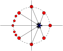
Figure 3: Three cycles mirror to the fractional branes in the resolution of $\mathbb{C}^{3}/\mathbb{Z}_{N}$.

The vector bundles in this geometry mirror to the $S^{3}$’s are shown in Fig. 3 and are given by [23, 24, 25, 26]:

$$F_{i}=(S^{-1})_{ji}{\cal O}(j)\,,$$ (42)

where [26]

$$S_{ij}=\chi({\cal O}(i),{\cal O}(j)) = 0\,,\,\,\mbox{if}\,\,i<j\,$$

$$= \#\{(m_{1},m_{2},m_{3})\,|\,m_{i}\geq 0,i-j=m_{1}+am_{2}+bm_{3}\}.$$

Then we see that

$$\chi(F_{i},{\cal O}(j)) = \delta_{ij}\,,$$ (44)

$$\chi(F_{i},F_{j}) = (S^{-1})_{ij}\,,$$

For a weighted projective space with weights $\{a_{1},a_{2},\cdots,a_{n}\}$ the generating function of the number of solitons is given by [26] as

$$F(q)=1+\sum_{I}n_{I}q^{I}=\prod_{i=1}^{n}(1-q^{a_{i}})\,.$$ (45)

The number of solitons between the $i$-th and the $j$-th vacua can be read from the above function as $n_{|i-j|}$. For the case we are interested in

$$F(q) = \prod_{k=1}^{3}(1-q^{a_{k}})=(1-q)(1-q^{a})(1-q^{b})\,,$$

$$= 1-q-q^{a}+q^{a+1}-q^{b}+q^{b+1}+q^{a+b}-q^{a+b+1}\,.$$

And this gives us the quiver diagram for each $i$ in Figure (4). Note that in the case $b=a+1$ (i.e., $N=2a+2$) there are bi-directional arrows related to nodes.

Figure 4: The $i$-th node of the quiver diagram for $\mathbb{C}^{3}/\mathbb{Z}_{N}$. We have marked all the nodes linked to $i$.

There are 8 terms in Equation (3.2) where the first term and the last term do not contribute to the quiver diagram and cancel each other since we identify the nodes modulo $N$. Now $F(1)=0$ implies the anomaly cancellation condition (the number of incoming and outgoing arrows being the same for each node). In general the mirror manifold is given by a (non-compact) genus $g$ fibration over the z-plane and a $\mathbb{C}^{\times}$ fibration over the z-plane. The genus $g$ fibration degenerates at $N=\chi(M)$ number of points on the z-plane where $M$ is compact divisor of $X$. In general $M$ will be a set of four manifolds $M_{i}$ joined together along some rational curves. The degeneration, of the genus $g$ fibration, is due to a 1-cycle collapsing. Using these collapsing 1-cycles one can construct 3-cycles, which are topologically $S^{3}$, in the mirror manifold $Y$.

Let us denote by $V_{a}$ the set of exceptional bundles on $M$ corresponding to the fractional branes,

$$\mbox{ch}(V_{a})=\{(r^{(a)}_{1},\cdots,r^{(a)}_{g}),(\Sigma^{(a)}_{1},\cdots,\Sigma^{(a)}_{g}),(k^{(a)}_{1},\cdots k^{(a)}_{g})\}\,,\,\,a=1,\cdots,N.$$

Where $r_{i}^{(a)}$ is the rank, $\Sigma^{(a)}_{i}$ the first Chern class and $k^{(a)}_{i}$ the second Chern character of the restriction of the bundle $V^{(a)}$ to $M_{i}$. Given this set of fractional branes the set of vanishing 1-cycles ${\cal C}_{a}$ is given by

$${\cal C}_{a}=\sum_{i=1}^{g}d_{\Sigma^{(a)}_{i}}\alpha_{i}+\sum_{i=1}^{g}r^{(a)}_{i}\beta_{j}\,\,,\,a=1,\cdots,N\,.$$ (47)

It follows then that the quiver diagram given by the intersection matrix of 3-cycles is

$$I_{ab}={\cal C}_{a}\cdot{\cal C}_{b}=\sum_{i=1}^{g}\mbox{det}\begin{pmatrix}d^{(a)}_{i}&d^{(b)}_{i}\\ r^{(a)}_{i}&r^{(b)}_{i}\end{pmatrix}\,.$$ (48)

And if the sum of the fractional branes is a D3-brane (0-cycle),

$$\sum_{a=1}^{N}\,r^{(a)}_{i}=\sum_{a=1}^{N}d_{\Sigma^{(a)}_{i}}=0\,,\,\forall i=1,\cdots,g\,.$$ (49)

then ${\cal C}=\sum_{a=1}^{N}{\cal C}_{a}$ is such that

$${\cal C}\cdot{\cal C}_{a}=0\,,\,\forall a=1,\cdots,N\,,$$ (50)

and gives rise to a $T^{3}$.

Example: $\mathbb{C}^{3}/\mathbb{Z}_{5}$:

We consider the case when $(a,b)=(2,2)$ (the other case of $(a,b)=(1,3)$ is equivalent to this one). In this case we have $\mathbb{P}^{2}_{[1,2,2]}$ as the weighted projective space collapsing to produce the orbifold singularity. The weighetd projective space itself has singularities which when resolved give the compact divisor $M$ as a $\mathbb{P}^{2}$ and $\mathbb{F}_{2}$ joined along a rational curve [25] as can be seen in the web diagram Figure (2). As discussed in the previous section the mirror Calabi-Yau is a genus two fibration and a $\mathbb{C}^{\times}$ fibration over the z-plane given by

$$W:=e^{u}+e^{v}+e^{-2u-2v}+e^{-t_{2}+\frac{3}{5}t_{1}-v} = z\,,$$ (51)

$$z+e^{t_{1}/5} = xy\,.$$

In the above equation $t_{1}$ and $t_{2}$ are the complexfied Kähler parameters. The genus two fibration degenerates at five points on the z-plane (depending on the Kähler parameters) as can be seen by solving the equations $\partial_{u}W=\partial_{v}W=0$. For $\lambda_{2}=e^{-t_{2}+(2/5)t_{1}}<<1$ the five degenerate fibers lie approximately on a circle in the z-plane and are, using Equation (47) and results of [25]

$$C_{1} = -\beta_{1}+2\beta_{2}\,,\,\,C_{2}=-\alpha_{1}-3\beta_{2}\,,\,\,C_{3}=4\beta_{1}+\alpha_{2}-\beta_{2}\,,$$ (52)

$$C_{4} = -\beta_{1}-\alpha_{2}\,,\,\,C_{5}=\alpha_{1}-2\beta_{1}+2\beta_{2}\,.$$

Given these cycles the quiver diagram can be obtained from the intersection numbers (see Figure (5)),

$$S_{a}\cdot S_{b}=C_{a}\cdot C_{b}\,.$$ (53)

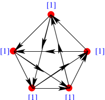
Figure 5: The quiver diagram of $\mathbb{C}^{2}/\mathbb{Z}_{5}$. Here we use $[1]$ to denote the rank of that node is 1.

4 Local del Pezzo Surfaces

4.1 Mirror Manifolds and Elliptic fibration

In this section we will consider non-compact Calabi-Yau threefolds which are line bundles over del Pezzo surfaces and their mirror partners. We will study the geometry of the mirror manifold in detail and see that results about classification of $[p,q]$ 7-branes in F-theory backgrounds actually allow us to write Diophantine equations, for all del Pezzo surfaces, whose solutions determine the quiver diagrams. We will see that these Diophantine equations derived from the geometry are the same as the equations given by the theory of solitons in ${\cal N}=(2,2)$ massive theories in two dimensions [21].

The superpotential of the LG theory mirror to the linear sigma model provides the description of mirror CY. Since $\mathbb{P}^{2}$ blown up at more than three points is not toric we cannot use the linear sigma model to obtain the mirror CY. However, it is possible to obtain the mirror manifolds $X_{k}$ to local non-toric del Pezzos $Y_{k}$ along the lines discussed in [7] using the fact that $\frac{1}{2}$-K3 ($\mathbb{P}^{2}$ blown up at nine points) is self-mirror [27]. The Calabi-Yau manifold mirror to local $\mathbb{B}_{k}$ ($\mathbb{P}^{2}$ blown up at $k$ points) is given by ($x,y,z,w_{1},w_{2}\in\mathbb{C}$)

$$y^{2} = x^{3}+f_{k}(z)x+g_{k}(z)\,,$$

$$w_{1}w_{2} = z-z_{*}\,,$$ (54)

where $f_{k}(z)$ and $g_{k}(z)$ are polynomials in $z$ and the explicit form of these polynomials can be found in [28]. The parameters in the polynomials $f_{k}$ and $g_{k}$ are the complex structure parameters of the mirror CY and are related to the Kähler structure parameters of the local del Pezzo.

The geometry of the mirror manifold $X_{k}$ is clear and is discussed in several papers [8, 10, 13]. We briefly mention it here again for completeness and because it will be useful for later discussion.

The first equation in (54) describes an elliptic fibration over the complex z-plane. This elliptic fibration has $k+3$ degenerate fibers whose positions depend on the Kähler parameters of the Calabi-Yau $Y_{k}$ or the complex structure parameters of $X_{k}$. The second equation in (54) describes a $\mathbb{C}^{*}$ fibration over the z-plane such that at $z=z_{*}$ the $\mathbb{C}^{*}$ fibration degenerates when its non-trivial $S^{1}$ shrinks.

The only non-trivial compact closed cycles in this geometry are 3-cycles. These 3-cycles are constructed as follows: we connect the point $z_{*}$ to the position of the degenerate fiber $z_{a}$, over this path we have 2-cycles which collapse at the two ends of this interval. The circle of the $\mathbb{C}^{*}$ fibration collapses at $z_{*}$ and a 1-cycle of the elliptic fibration collapses at $z_{a}$. These cycles together with the path in the z-plane form a closed 3-cycle which is topologically an $S^{3}$.

In this way we obtain $k+3$ 3-cycles with topology of $S^{3}$. This lattice of $k+3$ 3-cycles is mirror to $k+3$ dimensional lattice $H_{0}(\mathbb{B}_{k})\oplus H_{2}(\mathbb{B}_{k})\oplus H_{4}(\mathbb{B}_{k})$ of compact cycles in ${\cal B}_{k}$. The intersection between the 3-cycles is completely determined by the vanishing cycles of the elliptic fibration and the point $z_{*}$ can be thought of as the point from which the charges of the vanishing cycles are to be measured. This is quite reasonable since the only points at which the 3-cycle intersect lie on the elliptic fiber above the point $z=z_{*}$. Thus if the vanishing cycles are $C_{a}\equiv[p_{a},q_{a}]\in H_{1}(\pi^{-1}(z_{*}),{\sf Z\!\!\!Z})$ and the corresponding 3-cycles are $S_{a}$ then

$$S_{a}\cdot S_{b}:=C_{a}\cdot C_{b}=\mbox{det}\begin{pmatrix}p_{a}&p_{b}\\ q_{a}&q_{b}\,\end{pmatrix}.$$ (55)

Thus the information about the intersection numbers is naturally contained in the charges of the vanishing cycles of the elliptic fibration. Because of Picard-Lefschetz monodromy there is no unique choice of charges and by changing the paths connecting the position of degenerate fibers to $z_{*}$ we can change the charges.

A natural question is whether there is some invariant which characterizes this configuration of degenerate fibers. As discussed at length in [29] the only invariants of these configurations are the number of the degenerate fibers, the trace of the $SL(2,\mathbb{Z})$ monodromy matrix and the greatest common divisor of the intersection numbers. Actually one can write down Diophantine equations such that their solutions completely describe all the configurations which can be obtained by Picard-Lefschetz transformations as was done in [13] for the case of $Y_{0}$.

It is easy to understand the origin of such an equation. The monodromy matrix of a configuration of degenerate matrix is invariant under Picard-Lefschetz transformations but it is not invariant under global $SL(2,\mathbb{Z})$ transformation. However, the trace of the monodromy matrix is invariant under global $SL(2,\mathbb{Z})$ as well as Picard-Lefschetz transformations. The trace of the monodromy matrix does not depend on the vanishing charges and only depends on the intersection numbers between the vanishing charges [29]. The configuration of degenerate fibers we are considering are such that they have trace of the monodromy matrix equal to two. The implications of this were discussed at length in [29]. Thus the solutions of the equation

$$\mbox{det}(K_{\mathbb{B}_{k}}-1)=\mbox{Tr}K_{\mathbb{B}_{k}}-2=0\,,$$ (56)

except the trivial solution, completely describe different configurations related by Picard-Lefschetz transformations.

local $\mathbb{B}_{0}$:

This case was discussed in [13] where the Diophantine equation was also given but was derived using the relation of the local $\mathbb{B}_{0}$ mirror geometry with superpotential geometry of the mirror of the massive $\mathbb{P}^{2}$ model. We will show that these two points of view give the same equation in all local del Pezzo cases. The equation in this case is

$$\mu_{21}^{2}+\mu_{32}^{2}+\mu_{31}^{2}+\mu_{21}\mu_{32}\mu_{31}=0\,.$$ (57)

local $\mathbb{B}_{1}$ and local $\mathbb{F}_{0}$:

In both these cases the equation is given by

$$\mu_{21}^{2}+\mu_{31}^{2}+\mu_{41}^{2}+\mu_{32}^{2}+\mu_{42}^{2}+\mu_{43}^{2}+\mu_{21}\mu_{32}\mu_{31}\qquad\qquad$$ (58)

$$+\mu_{21}\mu_{42}\mu_{41}+\mu_{31}\mu_{43}\mu_{41}+\mu_{32}\mu_{43}\mu_{42}+\mu_{21}\mu_{32}\mu_{43}\mu_{41}=0\,.$$

In order to distinguish the two models, $\mathbb{B}_{1}$ and $\mathbb{F}_{0}$, we divide the solutions of the above equation in two sets. One set will have solutions with gcd equal to one giving the result for $\mathbb{B}_{1}$ and the other set has solutions with gcd equal to two giving the result for the $\mathbb{F}_{0}$ case. At this moment we do not know why $\mathbb{B}_{1}$ and $\mathbb{F}_{0}$ are distinguished by gcd. However, recalling the fact that $\mathbb{B}_{1}$ has only $SU(2)$ global flavor symmetry while $\mathbb{F}_{0}$ has $SU(2)\times SU(2)$ symmetry [18], we speculate that the symmetry maybe the reason behind. Similarly, we speculate that the fact that the gcd of $\mathbb{B}_{0}$ in all phases are always 3 is related to the $SU(3)$ global flavor symmetry.

local $\mathbb{B}_{k}$:

In the general case the equation is given by [29]

$$TrK-2=\sum_{r=2}^{k+3}\sum_{i_{1}>i_{2}>i_{3}\cdots>i_{r}}\mu_{i_{1}i_{2}}\mu_{i_{2}i_{3}}\cdots\mu_{i_{r-1}i_{r}}\mu_{i_{1}i_{r}} = 0\,.$$ (59)

Where $K$ is the monodromy matrix of a configuration of $k+3$ degenerate fibers.

¿From the above equation it is clear that if $\mu_{ij}=0$ for all $j$ and a fixed $i$ then the equation reduces to the Diophantine equation for $\mathbb{B}_{k-1}$. All solutions of the above equation are Picard-Lefshetz equivalent to the intersection numbers obtained from the following configuration,

$$\mu_{ij} = C_{i}\cdot C_{j}\,,$$ (60)

$$C_{i} = \alpha\,,\,i=1,\cdots,k\,,\,\,C_{k+1}=2\alpha-\beta\,,\,C_{k+2}=-\alpha+2\beta\,,\,\,C_{k+3}=-\alpha-\beta\,.$$

$\mathbb{C}^{3}/\mathbb{Z}_{5}$:

For $\mathbb{C}^{3}/\mathbb{Z}_{5}$ we can also write down a Diophantine equation whose solutions (except the trivial one) give the quiver diagram and the gauge group factors for all theories obtained from this geometry by Picard-Lefschetz transformation. If $M$ is the monodromy matrix around five degenerate fibers of a genus two fibration (given in terms of the charges of the degenerate fibers) then the Diophantine equation, which is function only of the intersection numbers, is given by

$$\mbox{det}(M-1\!\!1)=0\,.$$ (61)

The above equation simply means that the collection of degenerate fibers allow an eigenvector of eigenvalue one. Thus if the above equation is satisfied then there is a 1-cycle in the fibration which is invarinat under the monodromy and gives topologically a $T^{2}$ together with the path in the base that goes around the degenerate fibers. This $T^{2}$ together with the $S^{1}$ of the $\mathbb{C}^{\times}$ fibration gives a $T^{3}$. In the case of $\mathbb{C}^{3}/\mathbb{Z}_{3}$ and other local del Pezzo singularities the matrix $M$ is an $SL(2,{\sf Z\!\!\!Z})$ matrix and therefore since for an $SL(2,{\sf Z\!\!\!Z})$ matrix $\mbox{det}(M-1\!\!1)=2-\mbox{Tr}M$, the equation is given by $\mbox{Tr}M=2$ as discussed in the previous section.

It is easy to show that two solutions to Equation (61), which are related to each other by PL transformation, are given by

$$C_{1} = -\beta_{1}+2\beta_{2}\,,\,\,C_{2}=-\alpha_{1}-3\beta_{2}\,,\,\,C_{3}=4\beta_{1}+\alpha_{2}-\beta_{2}\,,$$ (62)

$$C_{4} = -\beta_{1}-\alpha_{1}\,,\,\,C_{5}=\alpha_{1}-2\beta_{1}+2\beta_{2}\,.$$

and

$$\widehat{C}_{1}=-C_{1}\,,\,\,\widehat{C}_{2}=C_{2}\,,\,\,\widehat{C}_{3}=C_{3}\,,\,\,\widehat{C}_{4}=C_{4}+2C_{1}\,,\,\,\widehat{C}_{5}=C_{5}+C_{1}\,.$$ (63)

On the z-plane the two solutions correspond to the 3-cycles shown in Figure (6) below.

Figure 6: Two solutions to the diphantine equation related to each other by PL transformation.

These two solutions are Seiberg dual to each other. The first solution gives a $\prod_{i=1}^{5}U(1)$ gauge theory with quiver given by Figure (7)(a). The second solution gives a $U(2)\times\prod_{i=1}^{4}U(1)$ gauge theory with quiver given by Figure (7)(b).

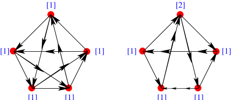
Figure 7: Two Seiberg dual quivers related to each other by Picard Lefschetz transformations.

$\mathbb{C}^{3}/\mathbb{Z}_{2k+1}$:

In this case we take the action of $\mathbb{Z}_{2k+1}$ on the $\mathbb{C}^{3}$ to be given by $(1,k,k)$. In this case the compact divisor of the resolved space is a $\mathbb{P}^{2}$ and $k-1$ Hirzebruch surfaces joined along the rational curves. The mirror is given by [9, 10]

$$e^{u}+e^{v}+e^{-ku-kv}+\sum_{m=1}^{k-1}\lambda_{m}e^{-mu-mv}=z\,,$$ (64)

$$z+e^{\frac{t_{0}}{2k+1}}=xy\,.$$

Where $\lambda_{m}$ are the complex structure parameters related to the Kähler parameters as $\lambda_{m}=e^{-t_{m}+\frac{t_{0}}{2m+1}}$. For $|\lambda_{m}|<<1$ we see that the critical points of the first equation above lie on a circle and the 3-cycles are as shown in Figure (8)(a). As we change the Kähler parameter $t_{0}$ we see that cycles undergo Picard-Lefschetz transformation as shown in Figure (8)(b). In this case also the intersection matrix of cycles will obey the Equation (61) with $M$ a $2k+1$ monodromy matrix given in terms of intersection numbers. However, in this case since there are more than one possible in equivalent resolutions of the singularity therefore not all solutions will be related by PL transformations. Thus it is necessary condition but not sufficient.

Figure 8: The two basis for the $\mathbb{C}^{3}/\mathbb{Z}_{2k+1}$.

Under the change in the basis of cycles shown in Figure (8)(b) the new basis is given by

$$S_{0} \mapsto \widehat{S}_{0}=-S_{0}\,,$$ (65)

$$S_{i} \mapsto \widehat{S}_{i}=S_{i}\,,\,\,i\neq 0,k+1,2k\,,$$

$$S_{k+1} \mapsto \widehat{S}_{k+1}=S_{k+1}+2S_{0}\,,$$

$$S_{2k} \mapsto \widehat{S}_{2k}=S_{2k}+S_{0}\,.$$

Where we have used the intersection numbers between the 3-cycles determined from the quiver diagram given by $F(q)=(1-q)(1-q^{k})^{2}$. Since $\sum_{a=0}^{2k}S_{a}=[T^{3}]$ therefore requiring the same for the new basis we get

$$\ \sum_{a=0}^{2k}n_{a}\widehat{S}_{a}=[T^{3}]\,\,\implies\,\,\,n_{0}=2,\,n_{i>0}=1\,.$$ (66)

Thus we get a $U(2)\times\prod_{i=1}^{2k}U(1)$ theory with quiver determined from $\widehat{S}_{a}\cdot\widehat{S}_{b}$. It is easy to check that the new quiver is indeed that of the Seiberg dual theory with duality performed on the $0-th$ node corresponding to $S_{0}$.

5 Seiberg Duality and Picard-Lefschetz Monodromy

The realisation that Seiberg’s duality can be geometricised as Picard-Lefschetz monodromy has been permeating in the literature since at least [14]. Recently works on Toric Duality [4, 5, 17, 16] have beckoned for a re-examination of the geometry of Seiberg duality. Indeed some ideas were presented in [17] and addressed in detail in [8, 13]. The purpose of this section is to explicit the derivation, as mentioned in [8], of Seiberg duality in terms of the quiver rules in [17] and point out some interesting examples in a comprehensive fashion. In due course we will resolve the discrepancies and puzzles which arose in [17] concerning the relation between Seiberg duality and Picard-Lefschetz theory. The relation between Seiberg duality and Picard-Lefshetz transformation was discussed in detail in [13] in terms of mutation of bundles and the corresponding action on the 3-cycles.

Instead of using the nomenclature of [17], we shall here use the language of $(p,q)$ 7-branes. As addressed in the earlier sections, the mirror picture of the transverse D-brane probe on $M$ consists of collections of (vanishing) three cycles $S_{i}$ with $n_{i}$ D-branes wrapped thereon in the mirror Calabi-Yau $W$. The result is a $\prod_{i}U(n_{i})$ gauge theory with bifundamentals $a_{ij}$ given as the intersection matrix of these vanishing cycles $S_{i}\cdot S_{j}$.

Now let us phrase these (Picard-Lefschetz) cycles $S_{i}$ in the language of $(p,q)$ 7-branes in the spirit of Section 2, emphasizing on the monodromy. Each $S_{i}$ can be represented by a $[p_{i},q_{i}]$ 7-brane together with a wrapping number $n_{i}$. The usual anomaly cancellation condition $\sum_{j}a_{ij}n_{j}=0$ now translates to

$$\sum\limits_{j}(S_{i}\cdot S_{j})n_{j}=0,\qquad\qquad\forall j.$$ (67)

In other words, the cycle $T=\sum\limits_{j}n_{j}S_{j}$ should have zero intersection with any cycle $S_{i}$. One particular case is that the cycle $T$ is precisely the $T^{3}$ fibre. As far as the $(p,q)$ charges are concerned, (67) is simply (see Equation (69))

$$\sum\limits_{i}n_{i}[p_{i},q_{i}]=0.$$ (68)

As mentioned earlier the bifundamental matter content is given by intersection numbers, which are computed as determinants. Strictly speaking, in the usual notation the adjacency matrix $a_{ij}$ of the quiver is such that $A_{ij}=a_{ij}-a_{ji}=S_{i}\cdot S_{j}$ where to distinguish them we have used $A_{ij}$ which can be both positive or negative. Through out the whole paper, except in Section 5.2, we assume that only one of $a_{ij},a_{ji}$ of a given pair $i,j$ is nonzero. Under this assumption, if $A_{ij}>0$ it is $a_{ij}\neq 0$ and if $A_{ij}<0$ it is $a_{ji}\neq 0$. The $A_{ij}$ is calculated as

$$A_{ij}=S_{i}\cdot S_{j}=\left|\begin{array}[]{cc}p_{i}&q_{i}\\ p_{j}&q_{j}\end{array}\right|.$$ (69)

Now Picard-Lefschetz monodromy is the motion of vanishing cycles $S_{j}$ about a chosen one $S_{i}$ such that thereafter the cycles becomes the linear combination (no summation on $i$)

$$S_{j}\rightarrow S_{j}+(S_{j}\cdot S_{i})S_{i}.$$

With wrapped branes the situation is a little more involved as we have to take into account how fractional branes rearrange in the new basis. Alternatively, one can take into account the usual brane creation mechanism [10, 13]. However before we elaborate on how to cooperate these factors in the following discussion, let us restate Picard-Lefschetz transformations in the language of $(p,q)$ charges:

Rules for Picard-Lefschetz on $(p,q)$ 7-branes

1. For a collection of vanishing cycles $S_{i}=[p_{i},q_{i}]$, each with wrapping number $n_{i}$, we let $S_{k-1}$ pass through $S_{k}$ for a chosen $k$.

2. All $S_{i}$ and $n_{i}$ for $i\neq k,k-1$ remain uneffected.

3. The concerned cycles transform as $S_{k-1}\rightarrow S_{k-1}+(S_{k-1}\cdot S_{k})S_{k}$ and $S_{k}\rightarrow S_{k}$, i.e.,

   $$\begin{pmatrix}p_{k-1}\\ q_{k-1}\end{pmatrix} \rightarrow \begin{pmatrix}p_{k-1}\\ q_{k-1}\end{pmatrix}+[Det\begin{pmatrix}p_{k-1}&q_{k-1}\\ p_{k}&q_{k}\end{pmatrix}]\begin{pmatrix}p_{k}\\ q_{k}\end{pmatrix}$$ (70)

   $$= \begin{pmatrix}1+p_{k}q_{k}&-p_{k}^{2}\\ q_{k}^{2}&1-p_{k}q_{k}\end{pmatrix}\begin{pmatrix}p_{k-1}\\ q_{k-1}\end{pmatrix};$$ (71)

   $$\begin{pmatrix}p_{k}\\ q_{k}\end{pmatrix} \rightarrow \begin{pmatrix}p_{k}\\ q_{k}\end{pmatrix}$$ (72)

4. The wrapping numbers transform as

   $$\begin{array}[]{cc}n_{k-1}\rightarrow n_{k-1};&n_{k}\rightarrow n_{k}-(S_{k-1}\cdot S_{k})n_{k-1}\end{array}$$

   If this new number $n_{k}$ is negative, we should simply make it positive and multiply the new $[p_{k},q_{k}]$ by $-1$. In geometric language, this changes the fractional brane into the anti-fractional brane as well as the orientation of the cycle $S_{k}$, so the net effect of (anti)-branes wrapping will be the same.

5. Now we have a new collection $(\widetilde{n_{i}},\widetilde{S_{i}})$ which is as before except for when $i=k,k-1$; these could then be used to calculate the new quiver $\widetilde{S_{i}}\cdot\widetilde{S_{j}}$.

As a check let us verify that the anomaly cancellation still holds. The condition (67) now reads

$$\sum_{i}\widetilde{n_{i}}\widetilde{S_{i}} = \sum_{i\neq k,k-1}n_{i}S_{i}+n_{k-1}(S_{k-1}+(S_{k-1}\cdot S_{k})S_{k}+(n_{k}-(S_{k-1}\cdot S_{k})n_{k-1})S_{k}$$

$$= \sum_{i}n_{i}S_{i}+n_{k-1}S_{k}(S_{k-1}\cdot S_{k})-(S_{k-1}\cdot S_{k})n_{k-1}S_{k}$$

$$= \sum_{i}n_{i}S_{i}$$

$$= 0,$$

which is as desired. The new quiver remains anomaly-free after any Picard-Lefschetz transformation.

5.1 Example: Hirzebruch Zero

After these generalities let us re-examine the by now familiar example of the cone over the zeroth Hirzebruch surface $\mathbb{F}_{0}$ [4, 5, 17, 13]. The two toric (Seiberg) dual cases are recapitulated in Figure (9). Our starting point is the following set of $(p,q)$ charges giving the affine $E_{1}$ background [29, 7]

$$A:~{}N+M_{1}~{}[1,-1]\qquad B:~{}N+M_{2}~{}[1,1]\qquad C:~{}N+M_{1}~{}[-1,1]\qquad D:~{}N+M_{2}~{}[-1,-1]$$

where $N,M_{1},M_{2}$ are all positive integers. This is the most general form of anomaly free theories on $\mathbb{F}_{0}$. Notice also that although we have three numbers $N,M_{1},M_{2}$, only two combinations, say $|M_{1}-M_{2}|$ and $N+min(M_{1},M_{2})$, are independent parameters. We can easily verify by computing pairwise determinants that the quiver is as given in Case (I).

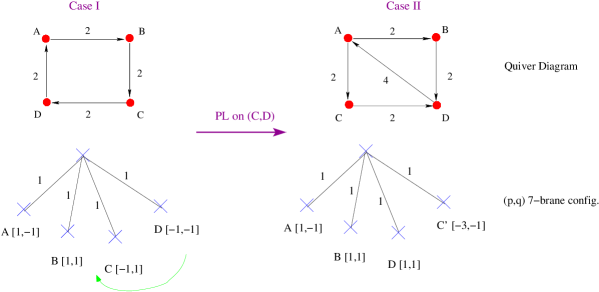
Figure 9: The toric (Seiberg) dual cases of the zeroth Hirzebruch surface $F_{0}$. Below the respective quiver diagrams we show the $(p,q)$ 7-brane configurations which give the quiver. Furthermore we see clearly how a Picard-Lefschetz transformation, as we move $D$ across $C$ in Case (I), gives Case (II).

If we move cycle $D$ past $C$, we will obtain the new configuration

$$A:~{}N+M_{1}~{}[1,-1]~{}~{}~{}~{}B:~{}N+M_{2}~{}[1,1]~{}~{}~{}~{}D:~{}n_{D}~{}[-1,-1]~{}~{}~{}~{}~{}C^{\prime}:~{}N+M_{1}~{}$$

where according to the rules above $A,B,D$ remain unchanged while

$$C\rightarrow C^{\prime}=\left[\begin{array}[]{cc}1+pq&-p^{2}\\ q^{2}&1-pq\end{array}\right]_{D}\left[\begin{array}[]{c}p\\ q\end{array}\right]_{C}=\left[\begin{array}[]{cc}2&-1\\ 1&0\end{array}\right]_{D}\left[\begin{array}[]{c}-1\\ 1\end{array}\right]_{C}=\left[\begin{array}[]{c}-3\\ -1\end{array}\right].$$

Moreover, the wrapping numbers are such that $n_{A},n_{B}$ and $n_{C^{\prime}}=n_{C}=N+M_{1}$ remain invariant, while

$$n_{D}\rightarrow n^{\prime}_{D}=n_{D}-(S_{C}\cdot S_{D})n_{C}=-N+M_{2}-2M_{1}$$ (73)

where we see that we still satisfy the zero charge (anomaly cancellation) condition, $\sum\limits_{i}n_{i}[p_{i},q_{i}]=0$. For the special case where $N=1,M_{1}=M_{2}=0$, we have $n^{\prime}_{D}=-1$. The negativity for $n^{\prime}_{D}$ indicates that we should reverse direction of the new 7-brane by changing the cycle into $[-p,-q]$. So finally we obtain the configuration

$$A:[1,-1]\quad B:[1,1]\quad D:[1,1]\quad C^{\prime}:[-3,-1]\qquad{\rm with}\quad n_{A}=n_{B}=n_{D}=n_{C^{\prime}}=1$$

Notice that under the above transformation, only the rank of node $D$ changed, so the node $D$ is exactly the node upon which we Seiberg dualise.

5.2 Deriving Seiberg Duality on one node from Picard-Lefschetz

First let us recall the rules for Seiberg duality on a single gauge group (single node) from the point of view of supersymmetric field theory. For clarification, we consider a general field theory with only bi-fundamental fields. We use $a_{ij}>0$ to denote the multiplicity of fields which are fundamental under $U(n_{i})$ and anti-fundamental under $U(n_{j})$. In the quiver diagram this means that there are $a_{ij}$ arrows starting from node $i$ and ending on node $j$. The steps of Seiberg duality are:

• (a) Pick up a node, for example $k$, to do Seiberg duality.

• (b) Ranks of all other nodes except node $k$ are invariant while that of $k$ becomes $N_{k}-n_{k}$ where $N_{k}=\sum_{i\neq k}n_{i}a_{ik}=\sum_{i\neq k}a_{ki}n_{i}$ is the total number of flavors for $U(n_{k})$.

• (c) Reverse the direction of arrows connected to node $k$. In field theory, this means that the dual quarks of the gauge group $U(N_{k}-n_{k})$ are in complex conjugate representations to the original quarks in representations of the gauge group $U(n_{k})$. Therefore $a_{ik}\rightarrow a_{ki},a_{kj}\rightarrow a_{jk}$.

• (d) Add the Seiberg mesons. If for given $i,j$ we have $a_{ik}\neq 0,a_{kj}\neq 0$, there are $m_{ij}=a_{ik}a_{kj}$ arrows starting from $i$ to $j$ (if $i=j$ they are adjoint fields). Thus the total number of arrows starting from $i$ to $j$ will be $a_{ij}+m_{ij}$.

• (e) Add the Seiberg superpotential of meson fields and dual quarks to the original superpotential with the original quarks fields replaced by meson fields. If there are fields which acquire mass, we simply integrate them out by their equations of motion.

Now the issue is how can we explain Seiberg duality from the geometrical Picard-Lefschetz transformations. Before doing so, there are a few points which are worth pointing out. First, Seiberg duality includes action on two parts: the matter part (quiver diagram) and the superpotential. At this moment, we can only reproduce the matter part by the geometric Picard-Lefschetz transformations. It will be interesting to derive the superpotential from these geometric transformations as well.

Second, even for the matter part, our understanding is not complete. The reason is that we calculate the quiver diagram by intersections of cycles in the mirror manifold. The intersection matrix captures only the antisymmetric part of the quiver diagram, i.e., we assume that one of $a_{ij},a_{ji}$ to be zero for any bi-directional pairs between nodes $i$ and $j$ as explained at the beginning of Section 5. It is important to note that only under these premises can we derive the matter part of Seiberg duality from geometric Picard-Lefshets transformation.

Now we show how to reproduce the matter part of Seiberg duality from geometric Picard-Lefschetz transformations, by comparison of the quiver duality rules above with those rules at the beginning of this section. We find that it is important to distinguish other nodes relative to the node $k$, the dualized node. In the spirit of [17], these nodes fall into three categories: the ones such that only $a_{ik}\neq 0$, the ones such that only $a_{kj}\neq 0$ and those with both $a_{ik}=a_{ki}=0$. For simplicity, we call them “Out”, “In” and “No” respectively. Furthermore, we make another important assumption: the order of cycles relative to cycle $S_{k}$ are as $S_{A\in Out},S_{k},S_{B\in In}$ while $S_{p\in No}$ can be anywhere. We do not know why this is a necessary condition, but from the derivation we can see it is indeed required for Picard-Lefschetz transformation to explain Seiberg duality. Other ordering would lead to Seiberg-like dualities, but not the simple Seiberg duality on a single node we are familiar with. Justifying this condition would be very interesting for the geometrisation of field theoretic dualities.

Now we proceed with the derivation. Under this condition of the ordering of cycles, we move $S_{k}$ all the way to the left hand side, passing through all the $S_{A}$ in the $Out$ category and possibly some $S_{p}$ in the $No$ category. We have the following transformation for each cycle in $A,B,p$:

$$S_{A} \rightarrow S_{A}+(S_{A}\cdot S_{k})S_{k}$$

$$S_{k,B,p} \rightarrow S_{k,B,p}$$

$$n_{k} \rightarrow n_{k}-\sum_{A\in Out}n_{A}(S_{A}\cdot S_{k})=n_{k}-N_{k}<0$$

$$n_{A,B,p} \rightarrow n_{A,B,p},$$

where the sum is accumulated as we move through each $Out$ cycle. The cycles $S_{p}$ do not change even if cycle $S_{k}$ has passed them because they have zero intersection number with $S_{k}$. Notice also that the quantity $\sum\limits_{A}n_{A}(S_{A}\cdot S_{k})$ is exactly the number of flavours $N_{k}$ with respect to the dualising node $k$. Now since $n_{k}-N_{k}<0$, according to our convention, the rank of the new gauge group should be $\widetilde{n_{k}}=N_{k}-n_{k}$ and the corresponding cycle should be $-S_{k}$. This reproduces rule (b) of Seiberg duality.

Next we need to calculate the quiver diagram by calculating the intersection of cycles. First $\widetilde{a_{ik}}=S_{i}\cdot(-S_{k})$, which implies that $\widetilde{a_{ik}}=-a_{ik}$. This explains the reversal of arrows connected to node $k$, i.e., rule (c). Second, we calculate $\widetilde{a_{ij}},i,j\neq k$. This part is modified only when at least one of $i,j$ is in the category “Out”. In this case, we have

$$\widetilde{S_{p}}\cdot\widetilde{S_{A}} = S_{p}\cdot S_{A}$$

$$\widetilde{S_{A}}\cdot\widetilde{S_{B}} = S_{A}\cdot S_{B}+(S_{A}\cdot S_{k})(S_{k}\cdot S_{B})$$

$$\widetilde{S_{A1}}\cdot\widetilde{S_{A2}} = S_{A1}\cdot S_{A2}$$

which exactly reproduces rule (d). In summary then we have derived Seiberg duality from Picard-Lefschetz.

5.3 An Interesting Question

Now we come to an interesting question. As we saw above, only in conjunction with the ordering of the cycles and making the special move of letting node $S_{k}$ pass through all nodes such that $(S_{i}\cdot S_{k})>0$, does Picard-Lefschetz monodromy derive Seiberg duality. Thus indeed the former is a more general class of phenomenon than the latter. This has been recently pointed out in [13] where Seiberg-like dualities were discussed.

If we do not pass through all nodes, what field theory is given by the transformation? We will see below that it is not a simple Seiberg Dual theory. It is important to figure out what is the physics behind such a perfectly well-defined procedure in geometrical engineering. To demonstrate this point, we continue with the above example of $\mathbb{F}_{0}$ (see Figure (10)). Starting from Case (I)

$$\begin{array}[]{ccccc}cycle:&A:[1,-1]&B:[1,1]&C:[-1,1]&D:[-1,-1]\\ n:&1&1&1&1\\ S_{i}\cdot S_{D}:&-2&0&2&0\\ \end{array}$$

Picard-Lefschetz transformation with respect to node D relative to C, we obtain Case (II)

$$\begin{array}[]{ccccc}cycle:&A:[1,-1]&B:[1,1]&D:[1,1]&C:[-3,-1]\\ n:&1&1&1&1\\ S_{i}\cdot S_{A}:&0&-2&-2&4\\ S_{i}\cdot S_{B}:&2&0&0&-2\\ S_{i}\cdot S_{D}:&2&0&0&-2\\ S_{i}\cdot S_{C}:&-4&2&2&0\\ \end{array}$$

These are the cases discussed earlier and presented in Figure (10).

If we move the node A relative to node C of phase II, we obtain case (III)

$$\begin{array}[]{ccccc}cycle:&C:[1,-5]&B:[1,1]&D:[1,1]&A:[-1,1]\\ n:&1&1&1&3\\ S_{i}\cdot S_{A}:&-4&2&2&0\\ S_{i}\cdot S_{B}:&6&0&0&-2\\ S_{i}\cdot S_{C}:&0&-6&-6&4\\ S_{i}\cdot S_{D}:&6&0&0&-2\\ \end{array}$$

which is Seiberg Dual to (II). However, if we dualise node C relative to node D of (II), we will obtain Case (IV)

$$\begin{array}[]{ccccc}cycle:&A:[1,-1]&B:[1,1]&C:[3,1]&D:[-5,-1]\\ n:&1&1&1&1\\ \end{array}$$

If we further transform node C relative to node B, we get Case (V)

$$\begin{array}[]{ccccc}cycle:&A:[1,-1]&C:[3,1]&B:[-5,-1]&D:[-5,-1]\\ n:&1&3&1&1\\ \end{array}$$

which is Seiberg dual to (II). We see that after two successive Picard-Lefschetz moves, we do obtain a Seiberg dual theory. This hints us that Picard-Lefschetz duality is a fractional Seiberg-duality. The various dualities are summarised in Figure (10).

Figure 10: The web of dualities one obtains for the zeroth Hirzebruch surface $\mathbb{F}_{0}$, as we perform Picard-Lefschetz moves on the corresponding $(p,q)$ 7-brane configurations.

6 Superpotential from Global Symmetries

We have seen that thusfar two alternative methods, one algebro-geometrical [13] and another combinatorial [4, 5], exists in the computation of the matter content and superpotential. The first problem of finding the quiver is relatively straight-forward and there exists yet another prescription using $(p,q)$-brane webs [8]. The superpotential on the other hand is rather involved: the $(p,q)$-description so far gives no direct technique, the exceptional bundle method requires involved Ext computations and the Inverse algorithm requires nontrivial integrating back.

The problem of finding an efficient method of determining the superpotential for classes of algebraic singularities remains a tantalising one. The following observations may yet point us to the right direction (q.v. [18] for discussions in a similar vein, especially on the third del Pezzo surface).

6.1 Example: $\mathbb{B}_{0}$

Let us proceed with the example of the cone over the zeroth del Pezzo surface, i.e., the blowup of the well-known orbifold $\mathbb{C}^{3}/\mathbb{Z}_{3}$ (cf. page 65 of [13]). Let us consider phase II of Figure 11. The 12 fields are arranged as 3 from node B to A, labelled as $\vec{X}$; 3 from node A to C, labelled as $\vec{Y}$ and 6 from node C to B, labelled as $Z_{ij}$. Now $SU(3)$ is the isometry group of $\mathbb{C}^{3}/\mathbb{Z}_{3}$, thus becomes a global symmetry group for the gauge theory. We expect the two triplets of fields ($\vec{X},\vec{Y}$) to be in irreducible representations of $SU(3)$ and we assign for convenience the anti-fundamental $\mathbf{\bar{3}}$ of $SU(3)$ while the sextuplet ($Z_{ij}$), to be in the symmetric 6 of $SU(3)$, an invariant scalar contraction is then obviously $X^{i}Y^{j}Z_{ij}$, which is precisely the superpotential computed by either algebraic methods or by performing Seiberg duality on phase I of Figure 11. In general we can follow the tree given in [13] modelling all the Seiberg dual theories of the above and arrive at Equation (31) for all the allowed number of fields $\mu_{21}$, $\mu_{32}$ and $\mu_{31}$ between nodes $12$, $23$ and $13$ respectively. (Here to compare to Figure 11 just make the replacements A by 1, B by 2 and C by 3). We expect such numbers to be all solutions for the ir(reducible) representations of $SU(3)$ and appropriate contractions then suffice.

6.1.1 Series of Theories for $\mathbb{B}_{0}$

The above is but one phase of a series of Seiberg duals of the theory [13, 17] and we made use of the explicit global $SU(3)$ flavour symmetry (also see [18]). We will now show that using this symmetry alone we can in fact write down the superpotential uniquely for many phases related to each other by Seiberg duality.

Let us start from model I in Figure 11. This is the toric phase [4]. In this model, we have 9 fields $X_{AB,i}$, $X_{BC,i}$ and $X_{CA,i}$ with $i=1,2,3$, all of which transform as the fundamental ${\bf 3}$ of the $SU(3)$ flavor symmetry. There is only one combination (tensor product as a Hom composition) of these to give a singlet of $SU(3)$, viz. , ${\bf 3}\otimes{\bf 3}\otimes{\bf 3}={\bf 1}+{\bf 8}+{\bf 8}+{\bf 10}$. Therefore, the only invariant scalar is given by

$$W_{I}=X_{AB,i}X_{BC,j}X_{CA,k}\epsilon^{ijk}.$$ (74)

This is of course the well-known superpotential [4, 13] for the toric phase of del Pezzo zero.

Now let us perform Seiberg duality with respect to node $A$. This model II is what was discussed above and in [17, 13]. We here discuss this example in detail to demonstrate our idea. First let us analyse the dual quarks. Under Seiberg duality, the fields $X_{AB,i}$ and $X_{CA,i}$ become $X_{BA}^{i}$ and $X_{AC}^{i}$. Therefore under the $SU(3)$, the ${\bf 3}$ changes to ${\bf\bar{3}}$. The fields $X_{BC,i}$ are invariant and remain as ${\bf 3}$. Next we need to add the meson fields $M_{CB,ij}$ which should transform under the tensor product ${\bf 3}\otimes{\bf 3}$. Since ${\bf 3}\otimes{\bf 3}={\bf 6}_{sym}+{\bf\bar{3}}_{antisym}$, we can write the meson fields into two irreducible representations $Y_{CB}^{i}$ for ${\bf\bar{3}}$ and $Y_{CB,(ij)}$ for ${\bf 6}$ where $(ij)$ means the symmetrisation of $ij$.

The subsequent superpotential of the dual field theory becomes $W^{\prime}=M_{CB,ij}X_{BC,j}\epsilon^{ijk}-M_{CB,ij}X_{BA}^{i}X_{AC}^{i}$ where the first term comes from $W_{I}$ and the second term comes from the duality. Notice that since $M_{CB,ij}\epsilon^{ijk}=Y_{CB}^{k}$, the first term in $W^{\prime}$ tells us that both fields $Y_{CB}^{k}$ and $X_{BC,i}$ are massive and should be integrated out. Using the equation of motion of fields $X_{BC,j}$ we find $Y_{CB}^{k}=0$ and the final superpotential is:

$$W_{II}=-X_{BA}^{i}X_{AC}^{j}Y_{CB,(ij)}.$$ (75)

The above result is derived from applying Seiberg duality rules in field theory. Now let us show how to use symmetry alone to reproduce this result. Under Seiberg duality, we have fields which transform under the following representations of $SU(3)$:

Field $$\mbox{Rep}(SU(3))$$

$$X_{BA}^{i} {\bf\bar{3}}$$

$$X_{AC}^{i} {\bf\bar{3}}$$

$$X_{BC,i} {\bf 3}$$

$$M_{CB,ij} {\bf 3}\otimes{\bf 3}={\bf 6}_{sym}+{\bf\bar{3}}_{anti}=Y_{CB,(ij)}+Y_{CB}^{i}$$

Whence we see that the fields $X_{BC,i}({\bf 3})$ will combine with fields $Y_{CB}^{i}({\bf\bar{3}})$ to become massive, so they can be integrated out. The remaining fields are ${\bf\bar{3}},{\bf\bar{3}}$ and ${\bf 6}$. Symmetry therefore tells us that there is only one flavor invariant superpotential we can write down:

$$W_{II}=X_{BA}^{i}X_{AC}^{j}Y_{CB,(ij)},$$

giving us the same results as (75) with much less work.

Next we dualize with respect to node $C$ to reach model III. In this case, the meson fields will be ${\bf 6}\otimes{\bf\bar{3}}:M_{AB,(ij)}^{k}$, which can be decomposed into ${\bf 15}+{\bf 3}$. The ${\bf 3}$ is given by the trace part $Y_{AB,j}=\sum_{i}M_{AB,(ij)}^{i}$ while the ${\bf 15}$ is given by the traceless part $Y_{AB,(ij)}^{k}$ with the condition $\sum_{k}Y_{AB,(kj)}^{k}=0$. As in model II, the ${\bf 3}$ field $Y_{AB,j}$ will be integrated out with ${\bf\bar{3}}$ field $X_{BA}^{i}$. Thus from these representations we find that the superpotential is uniquely determined as

$$W_{III}=Y_{BC}^{(ij)}X_{CA,k}Y_{AB,(ij)}^{k}.$$

Finally, we dualize on the node $A$ again to reach model IV. It is the first non-trivial example where the representation is not irreducible. The meson fields will be $M_{CB,(ij)k}^{l}={\bf 15}\otimes{\bf 3}$ which can be decomposed into ${\bf 24}+{\bf\overline{15}}+{\bf 6}$. The component of ${\bf 6}$ will become massive and be integrated out with fields $Y_{BC}^{(ij)}={\bf\bar{6}}$. This leaves us two irreducible components ${\bf 24}:Y_{CB,(ijk)}^{l}$ with $\sum_{k}Y_{CB,(ijk)}^{k}=0$ and ${\bf\overline{15}}:Y_{CB,k}^{(ij)}$ with $\sum_{k}Y_{CB,k}^{(kj)}=0$. The superpotential is determined again by the $SU(3)$ flavor symmetry as

$$W_{IV}=Y_{BA,l}^{(ik)}X_{AC}^{j}Y_{CB,k}^{(kl)}\epsilon_{ijk}+Y_{BA,l}^{(ij)}X_{AC}^{k}Y_{CB,(ijk)}^{l}.$$

We see therefore that by consideration of the representation theory of global symmetries, one could sometimes obtain the superpotential without recourse to the Inverse Algorithm or to helix methods.

Figure 11: The first few phases of $\mathbb{B}_{0}$ obtained by Seiberg duality. The letters A, B, C, label the gauge group. The numbers in square brackets are the ranks of the gauge groups.

The general prescription seems rather straight-forward, though the complete justification for this elegant technique still eludes us. We first identify the isometry of the singularity of concern, and then group the bi-fundamental fields into irreducible representations of this symmetry group. Contraction of these fields, now arranged as tensors of various rank, into a scalar, should give the final superpotential. Heuristically, this simply means that there is a remnant global symmetry, perhaps in the form of the centre of the Lie group, of the enhanced gauge symmetry which arise in the closed string sector as we compactify Type II on the appropriate Calabi-Yau cycles. The corresponding closed string moduli realise as gauge couplings in the open string sector which lives on the D-brane probe theory, some of which as coefficients of the terms in the superpotential, whereby giving our superpotentials surviving symmetries from the geometry.

Mathematically, the superpotential is a sum over all minimal loops in the quiver, weighted by the dimension of the Ext group of the various composition of the bundles in the exceptional collection. It is the non-zero terms that interest us. When the Ext-groups do not vanish should be precisely determined by the geometry of the Calabi-Yau base over which we have constructed the bundles.

6.2 del Pezzo Zero, Markov numbers and Helices

Let us examine the above case of the del Pezzo zero resolution of $\mathbb{C}^{3}/\mathbb{Z}_{3}$ in some more detail. As was pointed out in [13], if we let $(x,y,z)$ denote the number of bi-fundamentals between the nodes, then one can construct a tree of branching integer triplets which gives all allowed solutions under Seiberg duality.

Of course, as introduced earlier in Equation (31) and also in [21], the solutions are dictated by the Diophatine equation

$$x^{2}+y^{2}+z^{2}=xyz,$$ (76)

which we obtained from tracing over the product of monodromy matrices. On the other hand if we denote the rank of the nodes to be $(m,n,p)$, anomaly cancellation demands this triple to be in the nullspace of the intersection matrix. Whence, $\left(\begin{array}[]{ccc}0&x&-z\cr-x&0&y\cr z&-y&0\cr\end{array}\right)\left(\begin{array}[]{c}m\\ n\\ p\end{array}\right)=0$ and we immediately see the solution $(m,n,p)=a(y,z,x)$ for possibly fractional $a$ if $(x,y,z)$ were to have a common factor.

We recognise (76) as a case of the Hurwitz equation [34, 35], the general solution for which is given in [21]. One takes the fundamental solution $(3,3,3)$ and repeatedly applies $\left(\begin{array}[]{ccc}-1&1&1\cr 0&1&0\cr 0&0&1\cr\end{array}\right)$ in addition to the permutation $\Sigma_{3}$ on the triple. This generates the tree of solutions. One sees of course that they generate a braid group, in concordance with the fact that Seiberg duality is a monodromy action.

With the solution above, we see that the $(x,y,z)$ always have a common divisor of 3. This means that we can take the $a$ above to be $1/3$ and obtain the equation

$$m^{2}+n^{2}+p^{2}=3mnp$$ (77)

for the labels of the nodes. We recognize this to be the Markov equation [30]. The solutions for which are the renowned Markov numbers used in Diophantine approximation theory.

Indeed, we see that we are really dealing with only (77). Take (76), and consider it modolo 3. Because $2^{2}\equiv 1^{2}(\bmod 3)$, we only have to consider 4 possibilities on the left: $0+0+0$, $0+0+1$, $0+1+1$ or $1+1+1$. The second and third are instantly discarded because then the left would be non zero mod 3 while the right divides 3. The fourth is also impossible because the left would be 0 mod 3 and the right, not so. We conclude that the only solutions to (76) are when all $(x,y,z)$ are multiples of 3, whereupon we can instantly rename $(x,y,z)=(3m,3n,3p)$ and obtain (77). We summarise:

Theories related by Picard-Lefschetz duality (which are Seiberg duals) for the world-volume theory of D-branes probing the cone over del Pezzo zero are characterised by Markov numbers $(m,n,p)$: it is a $U(m)\times U(n)\times U(p)$ gauge theory with bifundamental matter $\left(\begin{array}[]{ccc}0&3p&-3n\cr-3p&0&3m\cr 3n&-3m&0\cr\end{array}\right)$.

One might wonder whether our Diophantine equation, derived from the monodromy matrix condition ${\rm Tr}K=2$, which is obviously necessary, is in fact sufficient to describe all solutions. We are saved by a result of Rudakov [31] which proved a 1-1 correspondence between the Fourier-Mukai vector of exceptional bundles on $\mathbb{P}^{2}$ related by mutations (or, in our language, the fractional brane charges on del Pezzo zero related by monodromy) and the Markov numbers. Therefore (77) does indeed characterise all solutions.

In a follow-up work [32], Rudakov addressed the case for $\mathbb{F}_{0}$. There, the statements are less powerful than the $\mathbb{P}^{2}$ case and a certain subset of the exceptional bundles are in bijection with $2x^{2}+y^{2}+z^{2}=4xyz$. The general problem of finding Diophatine equations characterising exceptional collections over arbitrary varieties remains open.

In fact over the $k$-th del Pezzo surface, the bundles are associated to the equation of the Markov type as:

$$ax^{2}+by^{2}+cz^{2}=\sqrt{K^{2}abc}\,xyz,$$

with $a,b,c$ integers and $K^{2}=9-k$ the intersection number of the canonical class [33]. The ranks of the what the authors define to be a triple of “three-blocks” of exceptional collections satisfy the above equation. The precise relation between this Diophantine equation and the ones discussed in Section 4 eludes us. It could well be that the fact that they coincide for the simplest case of $\mathbb{P}^{2}$ is mere coincidence.

7 Conclusions and Prospects

We have seen that dualities of quiver theories become geometric when these theories are realized in the Type IIA string theory using D6-branes. Although the superpotential is difficult to determine in these cases, in some aspects it seems that D6-brane picture is the more natural one. As we saw in the del Pezzo cases the geometry of the mirror manifold is able to provide Diophantine equations completely describing the various quiver diagrams related to each other by Picard-Lefschetz transformations. Parenthetically, works on helices on del Pezzo surfaces have also shown how exceptional collections could be classified by certain Diophantine equations. We have shown that in the case of $\mathbb{P}^{2}$ both prescriptions give the same Diophantine equation, namely the Markov equation. It would be enlightening to find out how they are related for the higher del Pezzos.

Moreover, it would be interesting to see if such equations exist for the theories arising via orbifolds. It is clear that the equations represent the necessary and sufficient condition for the existence of the $T^{3}$ mirror to the zero cycle. For example in the case of $\mathbb{C}^{3}/\mathbb{Z}_{5}$ orbifold the mirror manifold has five degenerate fibers of the genus two fibration so we need an equation which gives a necessary and sufficient condition for the existence of an eigenvector of the monodromy matrix around five degenerate fibers of a genus two curve. Such an equation will classify non-compact CY manifolds with two four cycles and Euler characteristic five similar to the classification of local del Pezzos from the elliptic curve [29].

As an aside we have shown in detail how with the imposition of certain condition one could derive Seiberg duality on the matter content of the quiver theory from Picard-Lefschetz moves; this is very much in the spirit of [13]. As an interesting by-product we have explicited an example where one obtains pairs of theories as a “fractional” generalisation of Seiberg duality. Of course the full treatment, incorporating the superpotential, still awaits a geometrical perspective. This should correspond to interesting behaviour in the field theory and seems to be a promising direction of pursuit.

Indeed whereas the transformation rules of the matter content under Seiberg duality are seen as a consequence of Picard-Lefschetz monodromy, the geometrisation of the superpotential transformation rules still needs full understanding. The current methods of computing superpotential, either from the Inverse Algorithm of [4, 5] for toric singularities, or from the composition of maps of sheafs [13], are computationally intensive. To have something akin to the elegant rules for the matter content for Seiberg duality or to determine the terms purely from global symmetries (isometries of the background geometry) would be a true blessing.

References

-
[1]
M. Douglas and G. Moore, “D-Branes, Quivers, and ALE
Instantons,” hep-th/9603167.
A. Lawrence, N. Nekrasov and C. Vafa, “On Conformal Field Theories in Four Dimensions,” Nucl. Physc. B533 (1998) 199-209, hep-th/9803015.
C. V. Johnson, R. C. Myers, “Aspects of Type IIB Theory on ALE Spaces,” Phys. Rev. D55 (1997) 6382-6393, hep-th/9610140.
A. Hanany and Y.-H. He, “Non-Abelian Finite Gauge Theories,” JHEP 9902 (1999) 013, hep-th/9811183.
A. Hanany and Y.-H. He, “A Monograph on the Classification of the Discrete Subgroups of SU(4),” JHEP 0102 (2001) 027, hep-th/9905212. - [2] E. Witten, “Phases of N=2 Theories In Two Dimensions,” Nucl. Phys. B403 (1993) 159-222, hep-th/9301042.
-
[3]
M. Douglas, B. Greene, and D. Morrison,
“Orbifold Resolution by D-Branes,” Nucl. Phys. B506 (1997) 84-106, hep-th/9704151.
P. S. Aspinwall, “Resolution of Orbifold Singularities in String Theory,” hep-th/9403123.
C. Beasley, B. R. Greene, C. I. Lazaroiu, and M. R. Plesser, “D3-branes on partial resolutions of abelian quotient singularities of Calabi-Yau threefolds,” Nucl. Phys. B566 (2000) 599-640, hep-th/9907186. - [4] B. Feng, A. Hanany, Y.-H. He, “D-Brane Gauge Theories from Toric Singularities and Toric Duality,” Nucl. Phys. B595 (2001) 165-200, hep-th/0003085.
- [5] B. Feng, A. Hanany, Y.-H. He, “Phase structure of D-brane gauge theories and toric duality,” JHEP 0108 (2001) 040, hep-th/0104259.
- [6] A. Iqbal, A. Neitzke and C. Vafa, ”A Mysterious Duality,” hep-th/0111068.
- [7] T. Hauer, A. Iqbal, “Del Pezzo Surfaces and Affine 7-brane Backgrounds,” JHEP 0001 (2000) 043, hep-th/9910054.
- [8] A. Hanany, A. Iqbal, “Quiver theories from D6-branes via mirror symmetry,” JHEP 0204 (2002) 009, hep-th/0108137.
- [9] K. Hori, C. Vafa, “Mirror Symmetry,” hep-th/0002222.
- [10] K. Hori, A. Iqbal, C. Vafa, “D-Branes And Mirror Symmetry,” hep-th/0005247.
- [11] F. Cachazo, S. Katz and C. Vafa, “Geometric transitions and N = 1 quiver theories,” hep-th/0108120.
- [12] F. Cachazo, K. Intriligator, C. Vafa, “A Large N Duality via a Geometric Transition,” Nucl. Phys. B603 (2001) 3-41, hep-th/0103067.
- [13] F. Cachazo, B. Fiol, K. Intriligator, S. Katz, C. Vafa, “A Geometric Unification of Dualities,” hep-th/0110028.
- [14] H. Ooguri, C. Vafa, “Geometry of N=1 Dualities in Four Dimensions,” Nucl. Phys. B500 (1997) 62-74, hep-th/9702180.
-
[15]
K. Dasgupta, K. Oh and R. Tatar, ”Geometric Transitions,
Large N Dualities and MQCD Dynamics,” Nucl. Phys. B610 (2001) 331-346, hep-th/0105066;
K. Oh and R. Tatar, ”Duality and Confinement in N=1 Supersymmetric Theories from Geometric Transitions,” hep-th/0112040. - [16] C. E. Beasley, M. R. Plesser, “Toric Duality Is Seiberg Duality,” JHEP 0112 (2001) 001, hep-th/0109053.
- [17] B. Feng, A. Hanany, Y. -H. He, A. M. Uranga, “Toric Duality as Seiberg Duality and Brane Diamonds,” JHEP 0112 (2001) 035, hep-th/0109063.
-
[18]
B. Feng, S. Franco, H. Hanany and Y.-H. He,
“Symmetries of Toric Duality,” hep-th/0205144;
T. Muto, “D-geometric Structure of Orbifolds,” hep-th/0206012. - [19] A. Strominger, S.-T. Yau, E. Zaslow, “Mirror Symmetry is T-Duality,” Nucl. Phys. B479 (1996) 243-259, hep-th/9606040.
- [20] K. Mohri, Y. Onjo, S. K. Yang, “Duality Between String Junctions and D-Branes on Del Pezzo Surfaces,” Nucl. Phys. B595 (2001) 138-164, hep-th/0007243.
- [21] S. Cecotti, C. Vafa, “On Classification of N=2 Supersymmetric Theories,” Commun. Math. Phy. 158 (1993) 569-644, hep-th/9211097.
- [22] C. Vafa, “Mirror Symmetry and Closed String Tachyon Condensation,” hep-th/0111051.
- [23] P. Mayr, “Phases of Supersymmetric D-branes on Kaehler Manifolds and the McKay correspondence,” JHEP 0101 (2001) 018, hep-th/0010223.
- [24] W. Lerche, P. Mayr, J. Walcher, “A new kind of McKay correspondence from non-Abelian gauge theories,” hep-th/0103114.
-
[25]
S. Mukhopadhyay, K. Ray, “Fractional Branes on a Non-compact
Orbifold”, JHEP 0107 (2001) 007, hep-th/0102146;
X. de la Ossa, B. Florea, H. Skarke, “D-branes on Noncompact Calabi-Yau Manifolds:K-Theory and Monodromy, hep-th/0104254. - [26] B. Acharya, C. Vafa, “On Domain Walls of N=1 Supersymmetric Yang-Mills in Four Dimensions,” hep-th/0103011.
- [27] J. A. Minahan, D. Nemeschansky, N. P. Warner, C. Vafa, “E-Strings and N=4 Topological Yang-Mills Theories,” Nucl. Phys. B527 (1998) 581-623, Nucl. Phys. B527 (1998) 581-623, hep-th/9802168.
- [28] A. Sen, B. Zwiebach, “Stable Non-BPS States in F-Theory,” JHEP 0003 (2000) 036, hep-th/9907164.
- [29] O. DeWolfe, T. Hauer, A. Iqbal, B. Zwiebach, “Uncovering Infinite Symmetries on [p,q] 7-branes: kac-Moody Algebras and Beyond,” Adv. Theor. Math. Phys. 3 (1999) 1835-1891, hep-th/9812209.
- [30] A. Markov, “Sur les Formes Quadratiques Binaires Indéfinites.” Math Ann 15 (1879).
- [31] A. Rudakov, “The Markov Numbers and exceptional bundles on ,” Math. USSR, Izv. 32, No.1 (1989).
- [32] A. Rudakov, “Exceptional Vector Bundles on a Quadric,” Math. USSR, Izv. 33 (1989).
- [33] B. Karpov and D. Nogin, “Three-block exceptional collections over Del Pezzo surfaces,” alg-geom/9703027.
- [34] A. Hurwitz, “Über Eine Aufgabe del Unbestimmten Analysis,” Archiv der Math. und Phys. 3 (14) 1907.
- [35] L. Mordell, “Diophantine Equations,” Academic Press, London 1969.