We construct explicit cohomogeneity two metrics of $G_{2}$ holonomy, which are foliated by twistor spaces. The twistor spaces are $S^{2}$ bundles over four-dimensional Bianchi IX Einstein metrics with self-dual (or anti-self-dual) Weyl tensor. Generically the 4-metric is of triaxial Bianchi IX type, with $SU(2)$ isometry. We derive the first-order differential equations for the metric coefficients, and obtain the corresponding superpotential governing the equations of motion, in the general triaxial Bianchi IX case. In general our metrics have singularities, which are of orbifold or cosmic-string type. For the special case of biaxial Bianchi IX metrics, we give a complete analysis their local and global properties, and the singularities. In the triaxial case we find that a system of equations written down by Tod and Hitchin satisfies our first-order equations. The converse is not always true. A discussion is given of the possible implications of the singularity structure of these spaces for M-theory dynamics.

1 Introduction

Concrete non-singular examples of seven-dimensional metrics with $G_{2}$ holonomy have been known only since about 1989. The original construction involved making an ansatz for metrics of cohomogeneity one, where the six-dimensional principal orbits were $S^{3}\times S^{3}$, or else the twistor spaces of $S^{4}$ or ${{\mathbb{C}}{\mathbb{P}}}^{2}$ [2, 4]. The twistor space is a 2-sphere bundle over the $S^{4}$ or ${{\mathbb{C}}{\mathbb{P}}}^{2}$ base, with an $SU(2)$ or $SO(3)$ structure group associated to the chiral spin (or spin^c) bundle of the base. The local construction can be carried out for any base space $M_{4}$ equipped with an Einstein metric and for which the Weyl tensor is self-dual or anti-self-dual [2, 4]. By a theorem of Hitchin, the only nonsingular such examples with positive Ricci tensor (which implies $M_{4}$ is compact) occur when $M_{4}$ is $S^{4}$ or ${{\mathbb{C}}{\mathbb{P}}}^{2}$ [6].

The current interest in $G_{2}$ manifolds in M-theory has been motivated in part by the role that they can play in compactifying to four dimensions, analogous to the compactification of ten-dimensional string theory on Calabi-Yau 6-manifolds. Unlike the latter, where non-singular Calabi-Yau manifolds can naturally give rise to chiral ${\cal N}=1$ theories in four dimensions starting from the heterotic string in $D=10$, non-singular $G_{2}$ compactifications of M-theory would necessarily give abelian non-chiral ${\cal N}=1$ theories in four dimensions. To get non-abelian chiral theories from M-theory, one needs to consider compactifications on singular $G_{2}$ manifolds. One explicit realisation of such an M-theory compactification has an interpretation as an $S^{1}$ lift of Type IIA theory (compactified on an orientifold) with intersecting D6-branes and O6 orientifold planes [8]. Non-Abelian gauge fields arise at the locations of coincident branes, and chiral matter arises at the intersections of D6-branes. The $S^{1}$ lift of such configurations results in singular $G_{2}$ holonomy metrics in M-theory. Co-dimension four ADE-type singularities are associated with the location of the coincident D6-branes, and co-dimension seven singularities are associated with the location of the intersection of two D6-branes in Type IIA theory [8, 10, 12, 13, 14].

Further analyses of co-dimension seven singularities of the $G_{2}$ holonomy spaces, leading to chiral matter, were given in [12, 13, 14] and the subsequent work [15, 16, 17, 18]. It is expected that there exist wide classes of 7-manifolds with $G_{2}$ holonomy and the singularity structure that again would yield non-Abelian ${\cal N}=1$ supersymmetric four-dimensional theories with chiral matter, and in particular the explicit construction of such metrics would provide a starting point for further studies of chiral M-theory dynamics.

Much research on finding new non-singular $G_{2}$ manifolds has been carried out in recent times (see, for example, [19, 20, 21, 22, 23, 24, 25] and references therein). In view of their potential phenomenological interest, it is appropriate also to investigate examples of singular $G_{2}$ manifolds. Typically, these singularities should be of co-dimension seven, and they should be of the relatively mild orbifold type [10, 12], where the curvature is bounded everywhere except for delta-function contributions.

One way to obtain singular $G_{2}$ holonomy spaces is by returning to the original $G_{2}$ construction in [2, 4], with principal orbits that are $S^{2}$ bundles over self-dual Einstein four-dimensional manifolds $M_{4}$ (forming the base of the twistor space), but with $M_{4}$ now chosen to be neither the $S^{4}$ nor the ${{\mathbb{C}}{\mathbb{P}}}^{2}$ non-singular examples. Instead, one can choose $M_{4}$ to be a self-dual Einstein space with orbifold-type singularities. Some investigations of the $G_{2}$ metrics that result from such a construction have already been carried out [16]. In this paper we pursue the analysis further, by considering more general possibilities for the base space $M_{4}$. Since the procedure for obtaining the $G_{2}$ metric from a given self-dual Einstein base space $M_{4}$ is well established [2, 4], much of the paper will concentrate on the details of the self-dual Einstein metrics themselves.

There exists a large mathematical literature on self-dual Einstein metrics (sometimes called quaternionic Kähler). The focus of our study in this paper will be on self-dual Einstein metrics of the triaxial Bianchi IX type, where there is an $SU(2)$ isometry that acts transitively on 3-dimensional orbits that are (locally) $S^{3}$. Quite a lot is known about this case [26, 28, 29], but we believe that our results go beyond what is in the existing literature, and that our viewpoint, derived as it is from the associated $G_{2}$ metric, is novel. In particular, we shall derive the general first-order equations for these metrics and analyse their local and global structure. For the special case of biaxial Bianchi IX metrics, we provide a complete analysis. In the triaxial case, we compare our analysis with that of Tod [27] and Hitchin [28, 29], and analyse some of the explicitly-known solutions. Some implications for M-theory of these $G_{2}$ holonomy metrics are also discussed.

2 Asymptotically-conical $G_{2}$ metrics

2.1 $G_{2}$ holonomy of $R^{3}$ bundles over self-dual Einstein 4-metrics

The metrics of $G_{2}$ holonomy that have twistor-space orbits take the form [2, 4]

$$ds_{7}^{2}=4\Big{(}1-{1\over r^{4}}\Big{)}^{-1}\,dr^{2}+r^{2}\,\Big{(}1-{1\over r^{4}}\Big{)}\,(D\mu_{i})^{2}+2r^{2}\,ds_{4}^{2}\,,$$ (1)

where $\mu_{i}\,\mu_{i}=1$. The covariant exterior derivative is defined by $D\mu_{i}\equiv d\mu_{i}+{\epsilon}_{ijk}\,A^{j}\,\mu_{k}$, and the metric $ds_{4}^{2}$ is required to be Einstein, with $R_{ab}=\Lambda\,g_{ab}$ (with $\Lambda$ taken to be normalised to $\Lambda=3$ in (1). The Yang-Mills fields have the defining property that $D\,J^{i}=0$, where the quaternionic Kähler forms $J^{i}$ on the base space M₄ have a definite duality, and satisfy

$$J^{i}_{ab}\,J^{j}_{bc}=-\delta_{ac}\,\delta^{ij}+{\epsilon}_{ijk}\,J^{k}_{ac}\,,$$ (2)

where the gauge-covariant exterior derivative is defined by

$$D\,J^{i}_{ab}\equiv\nabla\,J^{i}_{ab}+{\epsilon}_{ijk}\,A^{j}\,J^{k}_{ab}\,,$$ (3)

with

$$\nabla\,J^{i}_{ab}\equiv d\,J^{i}_{ab}+\omega_{ac}\,J^{i}_{cb}+\omega_{bc}\,J^{i}_{ac}\,.$$ (4)

The integrability condition $D^{2}\,J^{i}_{ab}=0$ has, as a particular consequence,

$$F^{i}_{ab}={\textstyle{{\scriptstyle 1}\over{\scriptstyle 2}}}J^{i}_{cd}\,R_{abcd}\,,$$ (5)

where $F^{i}\equiv dA^{i}+{\textstyle{{\scriptstyle 1}\over{\scriptstyle 2}}}{\epsilon}_{ijk}\,A^{j}\wedge A^{k}$. We furthermore require that the Yang-Mills fields $F^{i}$ be proportional to the quaternionic Kähler forms. We shall take $J^{i}_{ab}$ to be self-dual, in which case we have the identity

$$J^{i}_{ab}\,J^{i}_{cd}=\delta_{ac}\,\delta_{bd}-\delta_{ad}\,\delta_{bd}+{\epsilon}_{abcd}\,.$$ (6)

From this and equation (5), it can be seen that if the Weyl tensor

$$C_{abcd}\equiv R_{abcd}-{\textstyle{{\scriptstyle 1}\over{\scriptstyle 3}}}\Lambda\,(\delta_{ac}\,\delta_{bd}-\delta_{ad}\,\delta_{bc})$$ (7)

of the Einstein metric $ds_{4}^{2}$ is anti-self-dual, then we shall have

$$F^{i}={\textstyle{{\scriptstyle 1}\over{\scriptstyle 3}}}\Lambda\,J^{i}\,.$$ (8)

We can change variables to a set of coordinates $u_{i}$ on ${{\mathbb{R}}}^{3}$, which are unconstrained, by taking $u_{i}=\rho\,\mu_{i}$, and letting ${\textstyle{{\scriptstyle 1}\over{\scriptstyle 3}}}\Lambda\,\rho^{2}=r^{4}-1$, leading to the expression

$$ds_{7}^{2}={(Du_{i})^{2}\over\sqrt{1+{\textstyle{{\scriptstyle 1}\over{\scriptstyle 3}}}\Lambda\,\rho^{2}}}+2\sqrt{1+{\textstyle{{\scriptstyle 1}\over{\scriptstyle 3}}}\Lambda\,\rho^{2}}\,ds_{4}^{2}\,,$$ (9)

where $\rho$ means $\sqrt{u_{i}\,u_{i}}$, $D\,u_{i}=d\,u_{i}+{\epsilon}_{ijk}\,A^{j}\,u_{k}$, and we have rescaled so that $ds_{4}^{2}$ has cosmological constant $\Lambda$.

The $G_{2}$ holonomy is easily established by noting that we may take the associative 3-form to be, reverting to $\Lambda=3$ for convenience,

$$\Phi_{{\scriptscriptstyle(3)}}={\textstyle{{\scriptstyle 1}\over{\scriptstyle 6}}}(1+\rho^{2})^{-3/4}\,{\epsilon}_{ijk}\,Du_{i}\,Du_{j}\,Du_{k}+2(1+\rho^{2})^{1/4}\,Du_{i}\wedge J^{i}\,.$$ (10)

The dual of $\Phi_{{\scriptscriptstyle(3)}}$ in the metric (9) is therefore

$${*\Phi_{{\scriptscriptstyle(3)}}}=4(1+\rho^{2})\,\Omega_{{\scriptscriptstyle(4)}}+{\epsilon}_{ijk}\,Du_{i}\wedge Du_{j}\wedge J^{k}\,,$$ (11)

where $\Omega_{{\scriptscriptstyle(4)}}$ is the volume form of $ds_{4}^{2}$, which can also be written as $\Omega_{{\scriptscriptstyle(4)}}={\textstyle{{\scriptstyle 1}\over{\scriptstyle 2}}}J^{1}\wedge J^{1}={\textstyle{{\scriptstyle 1}\over{\scriptstyle 2}}}J^{2}\wedge J^{2}={\textstyle{{\scriptstyle 1}\over{\scriptstyle 2}}}J^{3}\wedge J^{3}$. From the identity $D^{2}\,u_{i}={\epsilon}_{ijk}\,F^{j}\,u_{k}$, one easily sees that $\Phi_{{\scriptscriptstyle(3)}}$ is closed and co-closed.

2.2 Nearly-Kähler geometry and $G_{2}$ holonomy

If we go to the asymptotic region, where $\rho\longrightarrow\infty$, we get the metric on the cone over the twistor space of M₄,

$$ds_{7}^{2}={1\over\rho}\,(Du_{i})^{2}+2\,\rho\,ds_{4}^{2}\,.$$ (12)

Defining $\rho={\textstyle{{\scriptstyle 1}\over{\scriptstyle 4}}}r^{2}$, this becomes

$$ds_{7}^{2}=dr^{2}+r^{2}\,ds_{6}^{2}\,,$$ (13)

and so if $ds_{7}^{2}$ has $G_{2}$ holonomy then

$$ds_{6}^{2}={\textstyle{{\scriptstyle 1}\over{\scriptstyle 4}}}(D\mu_{i})^{2}+{\textstyle{{\scriptstyle 1}\over{\scriptstyle 2}}}ds_{4}^{2}$$ (14)

is the nearly-Kähler metric on the twistor space of M₄. The associative 3-form becomes

$$\Phi_{{\scriptscriptstyle(3)}}={\textstyle{{\scriptstyle 1}\over{\scriptstyle 6}}}\rho^{-3/2}\,{\epsilon}_{ijk}\,Du_{i}\,Du_{j}\,Du_{k}+2\rho^{1/2}\,Du_{i}\wedge J^{i}\,,$$ (15)

and its Hodge dual is

$${*\Phi_{{\scriptscriptstyle(3)}}}=4\rho^{2}\,\Omega_{{\scriptscriptstyle(4)}}+{\epsilon}_{ijk}\,Du_{i}\wedge Du_{j}\wedge J^{k}\,.$$ (16)

The conditions of closure and co-closure of $\Phi_{{\scriptscriptstyle(3)}}$ therefore imply that $ds_{6}^{2}$ in (14) is nearly-Kähler.

The definition of a nearly-Kähler metric $ds_{6}^{2}$ is that the cone over $ds_{6}^{2}$, namely

$$d\hat{s}_{7}^{2}=dr^{2}+r^{2}\,ds_{6}^{2}\,$$ (17)

has $G_{2}$ holonomy. A more suggestive, but equivalent, terminology for $ds_{6}^{2}$ is therefore that it has weak $SU(3)$ holonomy; we discuss this briefly below.

If the cone metric $d\hat{s}_{7}^{2}$ has $G_{2}$ holonomy, it follows that the associative 3-form $\Phi_{{\scriptscriptstyle(3)}}$, which may be written as

$$\Phi_{{\scriptscriptstyle(3)}}=r^{2}\,dr\wedge J_{{\scriptscriptstyle(2)}}+r^{3}\,\rho_{{\scriptscriptstyle(3)}}\,,$$ (18)

must be closed and co-closed. This has the consequences

$$dJ_{{\scriptscriptstyle(2)}}=3\rho_{{\scriptscriptstyle(3)}}\,,\qquad d\tilde{\rho}_{{\scriptscriptstyle(3)}}+2J_{{\scriptscriptstyle(2)}}\wedge J_{{\scriptscriptstyle(2)}}=0\,,$$ (19)

where $\tilde{\rho}_{{\scriptscriptstyle(3)}}\equiv{*_{6}\rho_{{\scriptscriptstyle(3)}}}$. Immediate further consequences of these equations are $J_{{\scriptscriptstyle(2)}}\wedge\rho_{{\scriptscriptstyle(3)}}=0$ and $d\rho_{{\scriptscriptstyle(3)}}=0$. The associativity relation

$$\Phi_{ABE}\,\Phi_{CDE}=\delta_{AC}\,\delta_{BD}-\delta_{AD}\,\delta_{BC}+{\textstyle{{\scriptstyle 1}\over{\scriptstyle 6}}}{\epsilon}_{ABCDEFG}\,\Phi_{EFG}$$ (20)

for the 3-form $\Phi_{{\scriptscriptstyle(3)}}$ has the consequences that

$$J_{ab}\,J_{bc}=-\delta_{ac}\,,\qquad J_{ad}\,\rho_{abd}=\tilde{\rho}_{abc}\,.$$ (21)

This means that $J$ defines an almost complex structure in $ds_{6}^{2}$, and that with respect to $J$, $\psi_{{\scriptscriptstyle(3)}}\equiv\rho+{{\rm i}}\,\hat{\rho}$ is a holomorphic 3-form of type (3,0).

The relation to weak $SU(3)$ holonomy can be made more explicit by considering the covariantly-constant spinor $\hat{\eta}$ that exists in the $G_{2}$ metric (17). In the natural orthonormal basis $\hat{e}^{0}=dr$, $\hat{e}^{a}=r\,e^{a}$, one finds that the covariant exterior derivative $\hat{\nabla}=d+{\textstyle{{\scriptstyle 1}\over{\scriptstyle 4}}}\hat{\omega}_{AB}\,\Gamma^{AB}$ is given by $\hat{\nabla}=\nabla-{\textstyle{{\scriptstyle 1}\over{\scriptstyle 2}}}\Gamma_{0a}e^{a}+dr\,{\partial\over\partial r}$. If $ds_{6}^{2}$ has weak $SU(3)$ holonomy then it admits Killing spinors $\eta_{\pm}$ satisfying $D^{\pm}_{a}\,\eta_{\pm}\equiv(\nabla_{a}\pm{\textstyle{{\scriptstyle 1}\over{\scriptstyle 2}}}\Gamma_{0a})\,\eta_{\pm}=0$, for which the integrability condition is $[D^{\pm}_{a},D^{\pm}_{b}]={\textstyle{{\scriptstyle 1}\over{\scriptstyle 4}}}C_{abcd}\,\Gamma^{cd}$. This admits solutions $\eta_{\pm}$ if $C_{abcd}\,\Gamma^{cd}$ generates the $SU(3)$ subgroup of the tangent-space group $SO(6)\sim SU(4)$. The two spinors are related by $\eta^{*}_{\pm}=\eta_{\mp}$, and $\Gamma_{0}\,\eta_{\pm}=-\eta_{\mp}$. The covariantly constant spinor in the $G_{2}$ metric $d\hat{s}_{7}^{2}$ is given by $\hat{\eta}=\eta_{-}$.

In terms of the Killing spinors $\eta_{\pm}$ in $ds_{6}^{2}$, the almost complex structure $J_{{\scriptscriptstyle(2)}}$ and the 3-form $\rho_{{\scriptscriptstyle(3)}}$ are given by

$$J_{ab}={{\rm i}}\,\eta^{\dagger}_{+}\,\Gamma_{ab}\,\eta_{-}\,,\qquad\rho_{abc}={{\rm i}}\,\eta^{\dagger}_{+}\,\Gamma_{0abc}\,\eta_{-}\,.$$ (22)

From the Killing spinor equations $D^{\pm}_{a}\,\eta_{\pm}=0$ one can now easily derive the equations

$$\nabla_{a}\,J_{bc}=\rho_{abc}\,,\qquad\nabla_{a}\,\tilde{\rho}_{bcd}=-3J_{[ab}\,J_{cd]}\,.$$ (23)

These equations, which in particular imply (19), characterise nearly-Kähler metrics. Note that by symmetrising the first equation on $a$ and $b$, we obtain the equation for a Yano Killing tensor, $\nabla_{(a}\,J_{b)c}=0$ [30]. Thus the nearly Kähler 6-manifolds constructed in this paper provide new examples of a supersymmetric quantum mechanical systems with hidden symmetries [31, 32]. In fact, because $J_{ab}$ is an almost complex structure, the associated symmetric Staeckel Killing tensor is given by $J_{ab}\,J^{b}{}_{c}=-g_{ac}$, and hence is trivial in this case.

3 $G_{2}$ holonomy equations for Bianchi IX base

We now apply the formalism of section 2.1, with the four-dimensional base metric taken to be of the triaxial Bianchi IX form:

$$ds_{4}^{2}=dt^{2}+a_{i}^{2}\,\sigma_{i}^{2}\,.$$ (24)

The self-dual $SU(2)$ Yang-Mills connection is

$$A^{i}=-\omega_{0i}-{\textstyle{{\scriptstyle 1}\over{\scriptstyle 2}}}{\epsilon}_{ijk}\,\omega_{jk}\,,$$ (25)

where the spin connection of $ds_{4}^{2}$, in the vielbein basis $e^{0}=dt$, $e^{i}=a_{i}\,\sigma_{i}$, is given by

$$\omega_{01}=\beta_{1}\,e^{1}\,,\qquad\omega_{23}=\gamma_{1}\,e^{1}\,,$$ (26)

and cyclically, with

$$\beta_{1}\equiv-{\dot{a}_{1}\over a_{1}}\,,\qquad\gamma_{1}\equiv{a_{1}^{2}-a_{2}^{2}-a_{3}^{2}\over 2a_{1}\,a_{2}\,a_{3}}\,,$$ (27)

and cyclically. Since the Yang-Mills potentials are expressed in terms of the left-invariant 1-forms $\sigma_{i}$,

$$A^{i}=-a_{i}\,(\beta_{i}+\gamma_{i})\,\sigma_{i}\,,$$ (28)

the field strengths are necessarily $SU(2)$ invariant, and are given by

$$F^{i}=-\Theta_{0i}-{\epsilon}_{ijk}\,\Theta_{jk}\,.$$ (29)

By imposing the closure and co-closure of $\Phi_{{\scriptscriptstyle(3)}}$ given by (10) (or equivalently, and more simply, (15)), we find that the first-order equations for $a_{i}$ such that the 7-manifold has $G_{2}$ holonomy are then given by

$$\dot{a}_{1}-\dot{a}_{2}\,\dot{a}_{3}+\Big{(}{a_{3}^{2}-a_{1}^{2}-a_{2}^{2}\over 2a_{1}\,a_{2}}\Big{)}\,\dot{a}_{2}+\Big{(}{a_{2}^{2}-a_{1}^{2}-a_{3}^{2}\over 2a_{1}\,a_{3}}\Big{)}\,\dot{a}_{3}$$

$$\qquad\qquad\qquad+{a_{2}^{4}+a_{3}^{4}-3a_{1}^{4}+2(a_{1}^{2}\,a_{2}^{2}+a_{1}^{2}\,a_{3}^{2}-a_{2}^{2}\,a_{3}^{2}-{\textstyle{{\scriptstyle 2}\over{\scriptstyle 3}}}\Lambda\,a_{1}^{2}\,a_{2}^{2}\,a_{3}^{2}\,)\over 4a_{1}^{2}\,a_{2}\,a_{3}}=0\,,$$ (30)

together with the two equations obtained by cyclic permutation of the subscripts 1, 2 and 3. Note that we have restored the cosmological constant $\Lambda$, so that $ds_{4}^{2}$ satisfies $R_{ab}=\Lambda\,g_{ab}$. It is straightforward to see that after using the first-order equations, (29) becomes

$$F^{i}=-{\textstyle{{\scriptstyle 1}\over{\scriptstyle 3}}}\Lambda\,(e^{0}\wedge e^{i}+{\textstyle{{\scriptstyle 1}\over{\scriptstyle 2}}}{\epsilon}_{ijk}\,e^{j}\wedge e^{k})={\textstyle{{\scriptstyle 1}\over{\scriptstyle 3}}}\Lambda\,J^{i}\,.$$ (31)

We saw in in section 2 that the conditions for $ds_{7}^{2}$ in (9) to have $G_{2}$ holonomy should be equivalent to the conditions for $ds_{4}^{2}$ to have (anti)-self-dual Weyl tensor. In fact another way to derive the first-order equations (30) is as follows. We define the family of tensors

$$X_{abcd}\equiv R_{abcd}-\kappa\,(g_{ac}\,g_{bd}-g_{ad}\,g_{bc}\,,$$ (32)

where $\kappa$ is an as-yet unspecified constant parameter. If we now require that $X_{abcd}$ be anti-self-dual, we obtain the equation

$${}^{*}R_{abcd}+R_{abcd}-\kappa\,{\epsilon}_{abcd}-\kappa\,(g_{ac}\,g_{bd}-g_{ad}\,g_{bd})=0\,.$$ (33)

Contraction with $g^{bd}$ gives $R_{ac}=3\kappa\,g_{ac}$. It then follows that $X_{abcd}$ is the Weyl-tensor of an Einstein metric with scalar curvature $12\kappa$, and moreover that the Einstein manifold has anti-self-dual Weyl tensor. We find that the equations

$$X_{0123}=-X_{2323}\,,\qquad X_{0231}=-X_{3131}\,,\qquad X_{0312}=-X_{1212}$$ (34)

give precisely (30), and that the remaining anti-self-duality equations for $X_{abcd}$, i.e.

$$X_{0101}=-X_{0123}\,,\qquad X_{0202}=-X_{0231}\,,\qquad X_{0303}=-X_{0312}\,,$$ (35)

give second-order equations that are nothing but the derivatives of (30).

One could in principle solve (30) for the $\dot{a}_{i}$ themselves, but this involves finding the roots of a quintic equation. It is, nevertheless, useful to present the first-order equations in a factorised form. Solving two of the equations (30) for $\dot{a}_{2}$ and $\dot{a}_{3}$, and substituting into the third, we get

$$\Big{(}\dot{a}_{1}-{a_{1}^{2}-(a_{2}+a_{3})^{2}\over 2a_{2}\,a_{3}}\Big{)}^{2}\,\Big{(}\dot{a}_{1}-{a_{1}^{2}-(a_{2}-a_{3})^{2}\over 2a_{2}\,a_{3}}\Big{)}^{2}\Big{(}\dot{a}_{1}-{a_{1}^{2}-a_{2}^{2}-a_{3}^{2}\over 2a_{2}\,a_{3}}-{\textstyle{{\scriptstyle 1}\over{\scriptstyle 3}}}\Lambda\,a_{2}\,a_{3}\Big{)}$$

$$-{\textstyle{{\scriptstyle 1}\over{\scriptstyle 9}}}\Lambda^{2}\,a_{1}^{2}\,a_{2}\,a_{3}(2a_{2}\,a_{3}\,\dot{a}_{1}+3a_{2}^{2}+a_{3}^{2}-a_{1}^{2})(2a_{2}\,a_{3}\,\dot{a}_{1}+a_{2}^{2}+3a_{3}^{2}-a_{1}^{2})=0\,.$$ (36)

Of course the two equations following by cyclic permutation hold too, but it would be misleading to think of these three as the equations for the $a_{i}$, since one should not solve them independently. Rather, we can view (36) itself as the equation for $\dot{a}_{1}$, and then substitute this solution back into the cyclic set defined by (30) in order to obtain the equations for $\dot{a}_{2}$ and $\dot{a}_{3}$.

It is interesting to observe that in the limit when $\Lambda\longrightarrow 0$, then from (36) and (30) we can see that we get either the “Atiyah-Hitchin” [33] first-order system

$$\dot{a}_{1}={a_{1}^{2}-(a_{2}+a_{3})^{2}\over 2a_{2}\,a_{3}}\,,\qquad\hbox{and cyclic}\,,$$ (37)

or the “BGPP” [34] system

$$\dot{a}_{1}={a_{1}^{2}-a_{2}^{2}-a_{3}^{2}\over 2a_{2}\,a_{3}}\,,\qquad\hbox{and cyclic}\,.$$ (38)

The equations (37) admit the Atiyah-Hitchin [33] and self-dual Taub-NUT [35] metrics as particular solutions, whilst the equations (38) admit the BGPP [34] and Eguchi-Hanson [36] metrics as solutions.

It is often more convenient to recast first-order equations such as (30) into a form where the metric functions $\alpha_{i}\equiv a_{i}^{2}$ themselves appear without square roots. This can be achieved by introducing a new radial variable $\rho$, defined by $dt=a_{1}\,a_{2}\,a_{3}\,d\rho$. We then find that (30) becomes

$$2{d\alpha_{1}\over d\rho}-{1\over\alpha_{2}\,\alpha_{3}}\,{d\alpha_{2}\over d\rho}\,{d\alpha_{3}\over d\rho}+{(\alpha_{3}-\alpha_{1}-\alpha_{2})\over\alpha_{2}}\,{d\alpha_{2}\over d\rho}+{(\alpha_{2}-\alpha_{3}-\alpha_{1})\over\alpha_{3}}\,{d\alpha_{3}\over d\rho}$$

$$+\alpha_{2}^{2}+\alpha_{3}^{2}-3\alpha_{1}^{2}+2\alpha_{1}\,(\alpha_{2}+\alpha_{3})-2\alpha_{2}\,\alpha_{3}-{\textstyle{{\scriptstyle 4}\over{\scriptstyle 3}}}\,\Lambda\alpha_{1}\,\alpha_{2}\,\alpha_{3}=0\,,$$ (39)

and cyclically. Note also that in terms of the $\beta_{i}$ and $\gamma_{i}$ coefficients defined in (26) and (27), the first-order equations (30) can be written as

$$(\beta_{1}+\gamma_{1})\,(\gamma_{2}+\gamma_{3})=(\beta_{2}+\gamma_{2})\,(\beta_{3}+\gamma_{3})+{\textstyle{{\scriptstyle 1}\over{\scriptstyle 3}}}\Lambda\,,$$ (40)

and cyclically.

If we consider the specialisation where all three metric functions $a_{i}$ are set equal, $a_{i}=a$, the first-order system (30) reduces to

$$\dot{a}^{2}+{\textstyle{{\scriptstyle 1}\over{\scriptstyle 3}}}\Lambda\,a^{2}={\textstyle{{\scriptstyle 1}\over{\scriptstyle 4}}}\,.$$ (41)

This gives

$$ds_{4}^{2}=dt^{2}+{3\over 4\Lambda}\,\sin^{2}(\sqrt{{\textstyle{{\scriptstyle 1}\over{\scriptstyle 3}}}\Lambda}\,\,t)\,\sigma_{i}^{2}\,.$$ (42)

The metric extends to a complete non-singular metric on $S^{4}$ if $\Lambda>0$, and to the hyperbolic space $H^{4}$ if $\Lambda<0$.

The specialisation to biaxial metrics, where two of the metric functions are set equal, is considerably more complicated. We shall study this in detail in the next section.

4 Biaxial anti-self-dual Bianchi IX metrics

In this section we shall specialise to the biaxial case, setting $a_{2}=a_{1}$. The first-order equations (30) reduce to

$$\dot{a}_{3} = \dot{a}_{1}^{2}+{\dot{a}_{1}\,a_{3}\over a_{1}}-1+{3a_{3}^{2}\over 4a_{1}^{2}}+{\textstyle{{\scriptstyle 1}\over{\scriptstyle 3}}}\Lambda\,a_{1}^{2}\,,$$

$$0 = (2a_{1}\,\dot{a}_{1}+a_{3})(2a_{1}\,\dot{a}_{1}+a_{3}-2a_{1})(2a_{1}\,\dot{a}_{1}+a_{3}+2a_{1})+{\textstyle{{\scriptstyle 1}\over{\scriptstyle 6}}}\Lambda\,a_{1}(2a_{1}\,\dot{a}_{1}+3a_{3})\,.$$ (43)

It is easy to see that if we take the limit where $\Lambda$ goes to zero, the cubic equation for $\dot{a}_{1}$ has roots giving

$$\dot{a}_{1}=-{a_{3}\over 2a_{1}}+1\,,\quad\hbox{or}\quad\dot{a}_{1}=-{a_{3}\over 2a_{1}}-1\,,\quad\hbox{or}\quad\dot{a}_{1}=-{a_{3}\over 2a_{1}}\,.$$ (44)

The first two possibilities are associated with the first-order equations that yield the self-dual Ricci-flat Taub-NUT metrics, whilst the third yields the Eguchi-Hanson metric (which is also self-dual and Ricci-flat). In the self-dual Taub-NUT case, the $SO(3)\subset U(2)$ rotates the three hyper-Kähler forms as a triplet, while in the case of the Eguchi-Hanson metrics, they are singlets under $SO(3)$.

For future reference, we note that the equations (43) imply that the Weyl tensor of $ds_{4}^{2}$ satisfies the relation

$$Y^{2}=X^{3}\,,$$ (45)

where

$$X\equiv{\textstyle{{\scriptstyle 1}\over{\scriptstyle 24}}}C_{abcd}\,C^{abcd}\,,\qquad Y\equiv{\textstyle{{\scriptstyle 1}\over{\scriptstyle 48}}}C_{abcd}\,C^{cdef}\,C_{ef}{}^{ab}\,.$$ (46)

4.1 Self-dual Taub-NUT-de Sitter metrics

The general biaxial Bianchi IX Einstein metrics have long been known; these are the Taub-NUT-de Sitter solutions. Their local form can straightforwardly be derived by directly solving the Einstein equations in a suitable coordinate gauge. Writing (24) as

$$ds_{4}^{2}={dr^{2}\over a_{3}^{2}}+a_{1}^{2}\,(\sigma_{1}^{2}+\sigma_{2}^{2})+a_{3}^{2}\,\sigma_{3}^{2}\,,$$ (47)

the Ricci tensor is given (in the natural orthonormal frame) by

$$R_{00} = -a_{3}\,a_{3}^{\prime\prime}-{a_{3}^{\prime}}^{2}-{2(a_{1}^{\prime}\,a_{3}^{\prime}\,a_{3}+a_{1}^{\prime\prime}\,a_{3}^{2})\over a_{1}}\,,$$

$$R_{11} = R_{22}=-{a_{1}^{\prime\prime}\,a_{3}^{2}\over a_{1}}-{{a_{1}^{\prime}}^{2}\,a_{3}^{2}\over a_{1}^{2}}-{2a_{1}^{\prime}\,a_{3}^{\prime}\,a_{3}\over a_{1}}-{a_{3}^{2}\over 2a_{1}^{4}}+{1\over a_{1}^{2}}\,,$$ (48)

$$R_{33} = -a_{3}\,a_{3}^{\prime\prime}-{a_{3}^{\prime}}^{2}-{2a_{1}^{\prime}\,a_{3}^{\prime}\,a_{3}\over a_{1}}+{a_{3}^{2}\over 2a_{1}^{4}}\,.$$

From this we see that $R_{00}-R_{33}=-a_{3}^{2}\,(a_{1}^{-4}+4a_{1}^{\prime\prime}\,a_{1}^{-1})/2$, and since this must vanish by the Einstein condition, it is easy to solve for $a_{1}$, and hence, using the remaining Einstein equations, for $a_{3}$. Any Einstein solution to (48) is by definition a Taub-NUT-de Sitter metric. Apart from special limiting cases, the general solution has three parameters that we can think of as the mass $m$, the NUT charge $n$, and the cosmological constant $\Lambda$. This general metric is given by

$$ds_{4}^{2}={r^{2}-n^{2}\over\Delta}\,dr^{2}+{4n^{2}\,\Delta\over r^{2}-n^{2}}\,\sigma_{3}^{2}+(r^{2}-n^{2})\,(\sigma_{1}^{2}+\sigma_{2}^{2})\,,$$ (49)

where

$$\Delta\equiv r^{2}-2m\,r+n^{2}+\Lambda\,(n^{4}+2n^{2}\,r^{2}-{\textstyle{{\scriptstyle 1}\over{\scriptstyle 3}}}r^{4})\,.$$ (50)

The metric (49) has a self-dual or anti-self-dual Weyl tensor if [41]

$$m=\pm n\,(1+{\textstyle{{\scriptstyle 4}\over{\scriptstyle 3}}}\Lambda\,n^{2})\,,$$ (51)

in which case we find

$$\Delta=(r\mp n)^{2}\,(1-{\textstyle{{\scriptstyle 1}\over{\scriptstyle 3}}}\Lambda(r\mp n)(r\pm n))\,.$$ (52)

Making the specific choice of the upper sign, we obtain the self-dual Taub-NUT-de Sitter metric

$$ds_{4}^{2}={dr^{2}\over F}+4n^{2}\,F\,\sigma_{3}^{2}+(r^{2}-n^{2})\,(\sigma_{1}^{2}+\sigma_{2}^{2})\,,$$ (53)

where

$$F = \Big{(}{r-n\over r+n}\Big{)}\,(1-{\textstyle{{\scriptstyle 1}\over{\scriptstyle 3}}}\Lambda(r-n)(r+3n))\,,$$ (54)

$$= {\Lambda\over 3}\,\Big{(}{r-n\over r+n}\Big{)}\,(r_{+}-r)(r-r_{-})\,,\qquad r_{\pm}\equiv-n\pm\sqrt{4n^{2}+{3\over\Lambda}}\,.$$

The Weyl tensor is given by

$$C_{0101}=C_{2323}=-C_{0123}=-{n\,(1+{\textstyle{{\scriptstyle 1}\over{\scriptstyle 3}}}\Lambda\,n^{2})\over(r+n)^{3}}\,,$$

$$C_{0303}=C_{1212}=-C_{0312}={2n\,(1+{\textstyle{{\scriptstyle 1}\over{\scriptstyle 3}}}\Lambda\,n^{2})\over(r+n)^{3}}\,.$$ (55)

It can easily be verified that this metric satisfies the first-order equations (30). Note that because it is biaxial, and thus satisfies our reduced first-order system (43), it follows that the Weyl tensor of the self-dual Taub-NUT-de Sitter metrics obeys the relation (45). It is evident that if we send $\Lambda$ to zero in (53), we obtain the self-dual Taub-NUT metric first written down as a Euclidean-signature metric in [35]:

$$ds_{4}^{2}=\Big{(}{r+n\over r-n}\Big{)}\,dr^{2}+4n^{2}\,\Big{(}{r-n\over r+n}\Big{)}\,\sigma_{3}^{2}+(r^{2}-n^{2})(\sigma_{1}^{2}+\sigma_{2}^{2})\,.$$ (56)

We saw, however, that the first-order equations (43) have three branches, and in the limit where $\Lambda$ goes to zero two of these should lead to the self-dual Taub-NUT metric, whilst the third should lead instead to the Eguchi-Hanson metric. As noted above, the metric form (49) with parameters $m$, $n$ and $\Lambda$, and radial coordinate $r$, does not necessarily cover all regions of the modulus space, and in the present case the existence of three branches suggests that there should exist a different parameterisation of biaxial self-dual Einstein metrics whose limiting form when $\Lambda$ goes to zero is the Eguchi-Hanson metric.

The required metrics cannot be the ones found in [41], which are referred to as the Eguchi-Hanson-de Sitter metrics,

$$ds_{4}^{2}={dr^{2}\over F}+{\textstyle{{\scriptstyle 1}\over{\scriptstyle 4}}}r^{2}\,F\,\sigma_{3}^{2}+{\textstyle{{\scriptstyle 1}\over{\scriptstyle 4}}}r^{2}\,(\sigma_{1}^{2}+\sigma_{2}^{2})\,,$$ (57)

where $F=1-\ell^{4}\,r^{-4}-{\textstyle{{\scriptstyle 1}\over{\scriptstyle 6}}}\Lambda\,r^{2}$, because these metrics have neither self-dual nor anti-self-dual Weyl tensor, when $\Lambda$ and $\ell$ are both non-zero, and thus they do not satisfy (30). They are in fact Einstein-Kähler, and the Weyl tensor has a definite duality only if $\ell=0$ (giving the Fubini-Study metric on ${{\mathbb{C}}{\mathbb{P}}}^{2}$ if $\Lambda>0$, and the Bergmann metric on the open ball in ${{\mathbb{C}}}^{2}$ if $\Lambda<0$), or if $\Lambda=0$, in which case the Weyl tensor has the opposite duality and the metric is Eguchi-Hanson. In order to find the “missing” metrics, which we shall distinguish from (57) by giving them the name “self-dual Eguchi-Hanson-de Sitter,” it is helpful to study the first-order equations (43) in greater detail. This forms the topic of the next subsection.

4.2 Biaxial first-order equations, and self-dual Eguchi-Hanson-de Sitter

To proceed with studying the biaxial first-order equations (43), we define

$$u\equiv\dot{a}_{1}+{a_{3}\over 2a_{1}}\,.$$ (58)

The cubic equation for $\dot{a}_{1}$ now becomes

$$3u^{3}+(\Lambda\,a_{1}^{2}-3)\,u-\Lambda\,a_{1}\,a_{3}=0\,.$$ (59)

One approach is to follow Cardano’s procedure for solving the cubic equation, but other than establishing the principle that there will be two roots whose $\Lambda\longrightarrow 0$ limit yields the self-dual Taub-NUT first-order equation $u=\pm 1$, with the third yielding the Eguchi-Hanson first-order equation $u=0$ (see (44)), the direct solution of the cubic equation is not very enlightening.

A more profitable route is to view (59) as an equation expressing $a_{3}$ in terms of $u$,

$$a_{3}=-{u\,(u^{2}+\lambda\,a_{1}^{2}-1)\over\lambda\,a_{1}}\,.$$ (60)

Note that we are defining

$$\lambda\equiv{\textstyle{{\scriptstyle 1}\over{\scriptstyle 3}}}\Lambda$$ (61)

for convenience. In view of (60), we can now choose to regard $(a_{1},u)$ as our two metric functions, rather than $(a_{1},a_{3})$. From the first-order equations (43) we can now deduce that $a_{1}$ and $u$ satisfy the first-order equations

$$\dot{u}=-\lambda\,a_{1}\,,\qquad\dot{a}_{1}={u\,(u^{2}+3\lambda\,a_{1}^{2}-1)\over 2\lambda\,a_{1}^{2}}\,.$$ (62)

In order to find the solution that gives rise to Eguchi-Hanson in the $\lambda\equiv{\textstyle{{\scriptstyle 1}\over{\scriptstyle 3}}}\Lambda\longrightarrow 0$ limit, is useful to make a redefinition that casts the equations (62) and (60) into a form where this limit can be taken smoothly, and such that $u$ tends to zero in the limit. This is easily done, by letting $u=\lambda\,w$. The first-order equations (62) become

$$\dot{w}=-a_{1}\,,\qquad\dot{a}_{1}={w\,(\lambda^{2}\,w^{2}+3\lambda\,a_{1}^{2}-1)\over 2a_{1}^{2}}\,,$$ (63)

and (60) gives

$$a_{3}=-{w\,(\lambda^{2}\,w+3\lambda\,a_{1}^{2}-1)\over a_{1}}\,.$$ (64)

It follows that the solution to (63) for general non-vanishing $\lambda$ will give the required self-dual Eguchi-Hanson-de Sitter metrics. By defining a new radial variable $x$ such that $dx=-a_{1}\,dt$, the equation for $w$ can be solved to give $w=x$, and hence the solution for $a_{1}$ can be found. After a further simple coordinate redefinition, the solution can be expressed as

$$ds_{4}^{2}={d\rho^{2}\over U\,V}+{\textstyle{{\scriptstyle 1}\over{\scriptstyle 4}}}\rho^{2}\,{V\over 1-2\mu\,\ell^{2}}\,(\sigma_{1}^{2}+\sigma_{2}^{2})+{\textstyle{{\scriptstyle 1}\over{\scriptstyle 4}}}\rho^{2}\,\Big{(}{1-\mu\,\ell^{2}\over 1-2\mu\,\ell^{2}}\Big{)}^{2}\,U\,V\,\sigma_{3}^{2}\,,$$ (65)

where

$$U\equiv 1-{\ell^{4}\over\rho^{4}}\,,\qquad V\equiv 1-\mu\,(\ell^{2}+\rho^{2})\,.$$ (66)

The metric is Einstein, with cosmological constant $\Lambda=12\mu$, and its Weyl tensor is anti-self-dual. In fact, we find that the tangent-frame components of the Weyl tensor are given by

$$C_{0101}=C_{2323}=-C_{0123}=-{2\ell^{4}\,(1-\mu\,\ell^{2})\over\rho^{6}}\,,$$

$$C_{0303}=C_{1212}=-C_{0312}={4\ell^{4}\,(1-\mu\,\ell^{2})\over\rho^{6}}\,.$$ (67)

Since (65) is Einstein and of biaxial Bianchi IX type, it must be contained within the general Taub-NUT-de Sitter class of solutions (49). Furthermore, since its Weyl tensor is anti-self-dual, it can be expected to lie within the subclass of (49) that satisfy (51). After simple algebra we find that there is indeed a transformation that maps (49) with the anti-self-dual specialisation given by (51) into (65), namely

$$r^{2}=-{(12-\Lambda\,\ell^{2}-2\Lambda\,\rho^{2})^{2}\over 32\Lambda\,(6-\Lambda\,\ell^{2})}\,,\qquad n^{2}=-{(12-\Lambda\,\ell^{2})^{2}\over 32\Lambda\,(6-\Lambda\,\ell^{2})}\,.$$ (68)

Substituting these redefinitions into (49) with (52), we recover (63). It should be noted that when $\Lambda\,\ell^{2}<6$, the self-dual Eguchi-Hanson-de Sitter metric corresponds to a section of the self-dual Taub-NUT-de Sitter metric in which the NUT parameter and radial coordinate are imaginary. Thus from the point of view of the real geometry, the self-dual Taub-NUT-de Sitter and self-dual Eguchi-Hanson-de Sitter metrics should be viewed as inequivalent.

In order to clarify the relations between the self-dual Taub-NUT-de Sitter and self-dual Eguchi-Hanson-de Sitter metrics, and more generally to investigate the full solution space of the self-dual biaxial metrics, it is useful to study the phase-plane for the first-order system (62). Before doing so, we shall close this subsection by showing where two well-known self-dual Einstein metrics that are contained within the biaxial Bianchi IX class fit in, namely $S^{4}$ and ${{\mathbb{C}}{\mathbb{P}}}^{2}$.

Setting $\ell=0$ in (65) gives $S^{4}$, as can be seen by changing to the radial coordinate $t$ defined by $\sqrt{\mu}\,\rho=\sin{\textstyle{{\scriptstyle 1}\over{\scriptstyle 2}}}t$. This gives

$$ds_{4}^{2}={3\over\Lambda}\,(dt^{2}+{\textstyle{{\scriptstyle 1}\over{\scriptstyle 4}}}\sin^{2}t\,\sigma_{i}^{2})\,.$$ (69)

From (68), this corresponds to $n^{2}=-3/(4\Lambda)$ in the self-dual Taub-NUT-de Sitter parameterisation.

Another special case of (65), which arises when $\Lambda\,\ell^{2}=12$, also gives rise to $S^{4}$. This is a singular limit, for which we must first rescale the Euler angle $\psi$ that appears in $\sigma_{3}=d\psi+\cos\theta\,d\phi$ according to $\psi=(1-{\textstyle{{\scriptstyle 1}\over{\scriptstyle 12}}}\Lambda\,\ell^{2})^{-1}\,\tau$. Substituting into (65), and then sending $\ell^{2}\longrightarrow 12/\Lambda$, we obtain

$$ds_{4}^{2}={3\over\Lambda}\,[d\chi^{2}+\sin^{2}\chi\,(\sigma_{1}^{2}+\sigma_{2}^{2})+\cos^{2}\chi\,d\tau^{2}]\,,$$ (70)

where we have also set $\Lambda\,\rho^{2}=12\sin\chi$. We can recognise (70) as the metric on $S^{4}$, written as a foliation by $S^{2}\times S^{1}$ surfaces. The fact that (65) describes $S^{4}$ both for $\ell^{2}=0$ and $\ell^{2}=12/\Lambda$ is not unexpected in view of the expressions (67), since the Weyl tensor can be seen to vanish for these two values of $\ell^{2}$. Note that from (68) the value of NUT parameter in the self-dual Taub-NUT-de Sitter parameterisation corresponding to the $S^{4}$ limit with $\Lambda\,\ell^{2}=12$ is $n=0$.

A further special case of (65) is when $\Lambda\,\ell^{2}=6$. This gives ${{\mathbb{C}}{\mathbb{P}}}^{2}$. One must first define a new radial coordinate, for example by setting $\rho^{2}=(2\mu)^{-1}\,[1+(1-2\mu\,\ell^{2})\,\cos 2\chi]$, before taking the limit. We then obtain the metric

$$ds_{4}^{2}={6\over\Lambda}\,[d\chi^{2}+{\textstyle{{\scriptstyle 1}\over{\scriptstyle 4}}}\sin^{2}\chi\,(\sigma_{1}^{2}+\sigma_{2}^{2})+{\textstyle{{\scriptstyle 1}\over{\scriptstyle 4}}}\sin^{2}\chi\,\cos^{2}\chi\,\sigma_{3}^{2}]\,,$$ (71)

which can be recognised as the Fubini-Study metric on ${{\mathbb{C}}{\mathbb{P}}}^{2}$ [41]. From (68), it corresponds, in the self-dual Taub-NUT-de Sitter parameterisation, to sending the NUT parameter $n$ to infinity. Note that with the conventions of this paper, the Weyl tensor is anti-self-dual, as is the (covariantly constant) Kähler form $J=e^{0}\wedge e^{3}-e^{1}\wedge e^{2}$. Of course none of the self-dual quaternionic Kähler forms $J^{i}$ is covariantly constant, since the right-handed $SU(2)$ part of the spin connection is non-vanishing.

4.3 Phase-plane analysis for the biaxial system

As we have seen above, finding a uniform parameterisation of the space of solutions, even in the biaxial case, is non-trivial. The approach taken in this section will be to classify all the possible orbits in the phase space of the first-order equations (62). We shall find that not all solutions can be parameterised by giving real and finite values of $\ell$, or $n$.

We begin by making the definition $v=3a_{1}$, choosing the scale size $\lambda=3$ for convenience, and sending $t\longrightarrow-t$ for inconvenience. The first-order equations (62) become

$$\dot{u}=v\,,\qquad\dot{v}={9u\,(1-u^{2}-v^{2})\over 2v^{2}}\,,$$ (72)

and so the solutions can be represented as flows in the $(u,v)$ plane. We can divide the two equations to get

$${dv\over du}={9u\,(1-u^{2}-v^{2})\over 2v^{3}}\,.$$ (73)

In general, equation (73) can be integrated to give the flows for any biaxial self-dual solution. The constant of integration is related to the NUT parameter $n$, or, equivalently, the scale parameter $\ell$ in the self-dual Eguchi-Hanson-de Sitter formulation. In terms of $n$, the integral of (73) is given by

$$(u^{2}+{\textstyle{{\scriptstyle 1}\over{\scriptstyle 3}}}v^{2}-1)^{2}=12n^{2}\,(u^{2}+{\textstyle{{\scriptstyle 2}\over{\scriptstyle 3}}}v^{2}-1)\,.$$ (74)

Since this is symmetrical under reflections in the $u$ and $v$ axes, it suffices to consider flows within the positive quadrant.

It follows from (73) that flow lines inside the unit circle have positive gradient, whilst those outside the unit circle have negative gradient. The $v$ axis corresponds to $a_{3}=0$, signifying an endpoint of the metric at which the 3-dimensional orbits degenerate to an $S^{2}$ bolt. The $u$ axis, on the other hand, corresponds to $a_{1}=0$, and the metric will be singular here unless it happens that $u=\pm 1$ or $u=0$, in which case the orbits degenerate to a point, implying a NUT endpoint in the metric. By a theorem of Hitchin’s, the only complete and non-singular metrics with positive $\Lambda$ are $S^{4}$ and ${{\mathbb{C}}{\mathbb{P}}}^{2}$.

It is straightforward to establish that the ${{\mathbb{C}}{\mathbb{P}}}^{2}$ solution (71) corresponds to the ellipse $u^{2}+{\textstyle{{\scriptstyle 2}\over{\scriptstyle 3}}}v^{2}=1$. The flow starts on the $v$ axis at $v^{2}={\textstyle{{\scriptstyle 3}\over{\scriptstyle 2}}}$ at a bolt, and runs along the ellipse to a NUT on the $u$ axis at $u=1$. Since we have chosen the normalisation $\mu={\textstyle{{\scriptstyle 1}\over{\scriptstyle 12}}}\,\Lambda={\textstyle{{\scriptstyle 1}\over{\scriptstyle 4}}}\lambda={\textstyle{{\scriptstyle 3}\over{\scriptstyle 4}}}$ in this subsection, it follows that this occurs for $\ell^{2}={\textstyle{{\scriptstyle 2}\over{\scriptstyle 3}}}$.

The $S^{4}$ solution (69) with $\ell^{2}=0$ corresponds to the ellipse $(u-{\textstyle{{\scriptstyle 1}\over{\scriptstyle 2}}})^{2}+{\textstyle{{\scriptstyle 1}\over{\scriptstyle 3}}}v^{2}={\textstyle{{\scriptstyle 1}\over{\scriptstyle 4}}}$. This runs from the NUT at $u=0$, $v=0$ to the NUT at $u=1$, $v=0$. The other $S^{4}$ solution (70), with $\ell^{2}=12/\Lambda=4/3$, corresponds to the ellipse $u^{2}+{\textstyle{{\scriptstyle 1}\over{\scriptstyle 3}}}v^{2}=1$. Although this appears to be singular since, from (60), we have $a_{3}=0$, we saw that to obtain (70) it was necessary to rescale the $\psi$ coordinate and this has the effect of compensating for the vanishing of $a_{3}$.

The phase-plane plot, with the various ellipses and unit circle mentioned above displayed, is given in Figure 1.

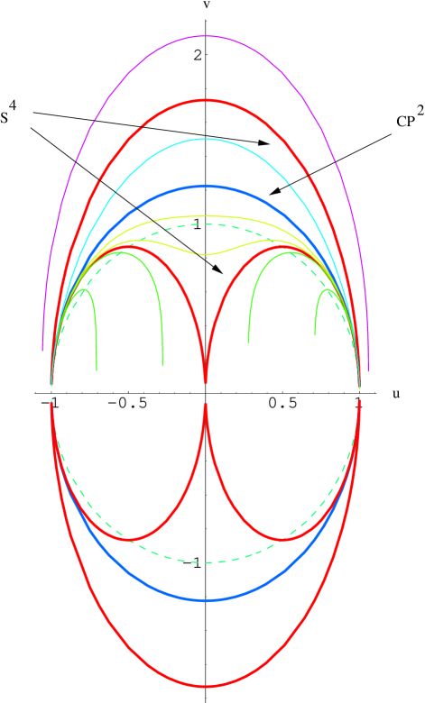
Figure 1: The phase plane for the first-order system of equation (72). The heavy blue ellipse corresponds to the ${{\mathbb{C}}{\mathbb{P}}}^{2}$ flow, and the three heavy red ellipses to $S^{4}$ flows. The dashed green circle is $u^{2}+v^{2}=1$; all solutions that cross this do so horizontally. To label distinct metrics it is sufficient to consider flows lying within the positive quadrant. We label qualitatively similar flows by A, B, C and D, which indicate the regions they occupy and their initial points. Thus the regions A, B and C indicate starting-points for solutions on the $v$ axis. Region A ranges from $v=0$ to the intersection of the ${{\mathbb{C}}{\mathbb{P}}}^{2}$ ellipse with the $v$ axis. Region B ranges from this intersection to the intersection of the outer ellipse (the $S^{4}$ solution (70)) with the $v$ axis. Region C ranges from this point to $v=+\infty$. Region D denotes (singular) starting points on the $u$ axis for solutions, in the range $0<u<1$. For clarity we have plotted complete ellipses for the $S^{4}$ an ${{\mathbb{C}}{\mathbb{P}}}^{2}$ special cases, but only flows in the upper half-plane for the other representative examples.

From (74), we see that solutions starting from a bolt on the $v$ axis are specified at $u=0$ by

$$\hbox{\bf Region A}: -\infty<n^{2}<-{\textstyle{{\scriptstyle 1}\over{\scriptstyle 12}}}:\qquad\qquad{\textstyle{{\scriptstyle 3}\over{\scriptstyle 2}}}>v^{2}>0\,,$$

$$\hbox{\bf Region B}: -\infty<n<0:\qquad\qquad{\textstyle{{\scriptstyle 3}\over{\scriptstyle 2}}}<v^{2}<3\,,$$

$$\hbox{\bf Region C}: 0<n<\infty:\qquad\qquad 3<v^{2}<\infty\,.$$

We also have solutions starting from the singular curvature singularity along the $u$ axis, specified at $v=0$ by:

$$\hbox{\bf Region D}:\qquad-{\textstyle{{\scriptstyle 1}\over{\scriptstyle 12}}}<n^{2}<0:\qquad\qquad 0<u<1\,.$$ (75)

In terms of the parameter $\ell^{2}$ of the self-dual Eguchi-Hanson-de Sitter formulation of the metrics, we see from (68) that Region A, where $n$ is imaginary, is covered by real values of $\ell$, and so the self-dual Eguchi-Hanson-de Sitter form of the metrics is better adapted to describing this region of the phase plane. On the other hand, in Region D, where $n$ is again imaginary, $\ell$ is complex, and so neither the self-dual Taub-NUT-de Sitter nor self-dual Eguchi-Hanson-de Sitter formulation is well adapted to describing this region of the phase plane. It is straightforward to find an adapted parameterisation where the analogue of the NUT parameter, and the radial coordinate, is real in Region D, but since the metrics there have power-law curvature singularities there is not much value in writing them down.

It is instructive to express the Weyl tensor for the biaxial self-dual metrics in terms of $u$ and $v$. We find that it is given by

$$C_{0101}=-C_{0123}=C_{2323}=-2C_{0303}=2C_{0312}=-2C_{1212}=f\,,$$ (76)

where

$$f=-{\textstyle{{\scriptstyle 81}\over{\scriptstyle 2}}}\,v^{-6}\,(u^{2}+{\textstyle{{\scriptstyle 1}\over{\scriptstyle 3}}}v^{2}-1)\,\Big{(}(u-{\textstyle{{\scriptstyle 1}\over{\scriptstyle 2}}})^{2}+{\textstyle{{\scriptstyle 1}\over{\scriptstyle 3}}}v^{2}-{\textstyle{{\scriptstyle 1}\over{\scriptstyle 4}}}\Big{)}\,\Big{(}(u+{\textstyle{{\scriptstyle 1}\over{\scriptstyle 2}}})^{2}+{\textstyle{{\scriptstyle 1}\over{\scriptstyle 3}}}v^{2}-{\textstyle{{\scriptstyle 1}\over{\scriptstyle 4}}}\Big{)}\,.$$ (77)

As expected, this vanishes only on the $S^{4}$ ellipses, and it diverges everywhere on the $u$ axis except at the points $u=0,\pm 1$, provided they are approached along the $S^{4}$ flows.

4.4 Global structure of the biaxial solutions

As we have already remarked, a theorem of Hitchin’s implies that when the cosmological constant $\Lambda$ is positive, only the $S^{4}$ and ${{\mathbb{C}}{\mathbb{P}}}^{2}$ self-dual Einstein metrics can be non-singular. In particular, therefore, this means that the self-dual Taub-NUT-de Sitter and self-dual Eguchi-Hanson-de Sitter metrics will be singular except for the special values of $n$ or $\ell^{2}$ for which they reduce to $S^{4}$ or ${{\mathbb{C}}{\mathbb{P}}}^{2}$.

We shall analyse the self-dual Taub-NUT-de Sitter metrics first, described by (53) and (54). The coordinate $r$ is taken to lie in the interval $n\leq r\leq r_{+}$. For convenience, we shall again set $\Lambda=9$ here. Near $r=n$, letting $r-n=\rho^{2}$, the metric becomes

$$ds_{4}^{2}\sim 8n\,[d\rho^{2}+{\textstyle{{\scriptstyle 1}\over{\scriptstyle 4}}}\rho^{2}\,(\sigma_{1}^{2}+\sigma_{2}^{2}+\sigma_{3}^{2})]\,,$$ (78)

which describes a NUT. The metric smoothly approaches the origin of ${{\mathbb{R}}}^{4}$, provided that the Euler angle $\psi$ appearing in $\sigma_{3}=d\psi+\cos\theta\,d\phi$ has its canonical period $4\pi$.

Near $r=r_{+}$, by letting $r_{+}-r=\rho^{2}$ we see that the metric becomes

$$ds_{4}^{2}\sim{2\over(\sqrt{3}\sqrt{12n^{2}+1}-6n)}\,(d\rho^{2}+4n^{2}\,(\sqrt{3}\sqrt{12n^{2}+1}-6n)^{2}\,\rho^{2}\,\sigma_{3}^{2})+(r_{+}^{2}-n^{2})\,(\sigma_{1}^{2}+\sigma_{2}^{2})\,.$$ (79)

This approaches ${{\mathbb{R}}}^{2}\times S^{2}$ locally, but in general there will be a conical singularity. If $\psi$ has period $\Delta\psi=4\pi/N$, then regularity at $r=r_{+}$ is achieved if

$$N=4n(-6n+\sqrt{3}\sqrt{12n^{2}+1})\,.$$ (80)

Regularity at $r=n$ required $N=1$. This is compatible with (80) if $n=\infty$, which is the limit where the self-dual Taub-NUT-de Sitter metric becomes ${{\mathbb{C}}{\mathbb{P}}}^{2}$ [41]. (Another case where the singularity can be avoided is by taking a limit where $n^{2}\longrightarrow-3/(4\Lambda)=-{\textstyle{{\scriptstyle 1}\over{\scriptstyle 12}}}$, in which case one must first rescale coordinates in the metric. This case is $S^{4}$.) For all other values of $n$, there will be a deficit angle at the origin, and a hence a conical singularity.

The $G_{2}$ metrics (9) obtained by taking $ds_{4}^{2}$ to be self-dual Taub-NUT-de Sitter were discussed recently in [16]. They have cohomogeneity 2, since there are two “radial” coordinates $\rho$ and $t$. The conical singularities in the Taub-NUT-de Sitter metrics imply, of course, that the corresponding $G_{2}$ metrics will have conical singularities too.

A further class of geometries within the biaxial Bianchi IX class is obtained by considering instead the self-dual Eguchi-Hanson-de Sitter form of the metrics, given by (65). If $2\mu\,\ell^{2}<1$, meaning that $\Lambda\,\ell^{2}<6$, the radial coordinate $\rho$ can be chosen to lie in the interval $\ell\leq\rho\leq\rho_{0}$, where $\rho_{0}^{2}=1/\mu-\ell^{2}$. Near $\rho=\ell$, setting $\rho=\ell+x^{2}$, we find

$$ds_{4}^{2}\sim{\ell\over 1-2\mu\,\ell^{2}}\,[dx^{2}+(1-\mu\,\ell^{2})^{2}\,x^{2}\,\sigma_{3}^{2}]+{\textstyle{{\scriptstyle 1}\over{\scriptstyle 4}}}\ell^{2}\,(\sigma_{1}^{2}+\sigma_{2}^{2})\,,$$ (81)

whilst near $\rho=\rho_{0}$, we have, setting $\rho=\rho_{0}-x^{2}$,

$$ds_{4}^{2}\sim{1-\mu\,\ell^{2}\over 1-2\mu\,\ell^{2}}\,(dx^{2}+{\textstyle{{\scriptstyle 1}\over{\scriptstyle 4}}}x^{2}\,\sigma_{i}^{2})\,.$$ (82)

Thus regularity at the NUT at $\rho=\rho_{0}$ requires that $\psi$ have period $4\pi$, which implies that there is a conical singularity on the bolt at $\rho=\ell$.

4.5 Phase plane and global structure for negative $\Lambda$

The phase-plane analysis of section 4.3 can be repeated for the case where the cosmological constant $\Lambda$ is taken to be negative. Starting from (62) and (60), and fixing the scale by choosing $\lambda\equiv{\textstyle{{\scriptstyle 1}\over{\scriptstyle 3}}}\Lambda=-3$, we now have

$$\dot{u}=v\,,\qquad\dot{v}={9u\,(1-u^{2}+v^{2})\over 2v^{2}}\,,$$

$${dv\over du}={9u\,(1-u^{2}+v^{2})\over 2v^{3}}\,,$$

$$a_{3}=-{u\over v}\,(1-u^{2}+{\textstyle{{\scriptstyle 1}\over{\scriptstyle 3}}}v^{2})\,.$$ (83)

The flow can be integrated, giving

$$(u^{2}-{\textstyle{{\scriptstyle 1}\over{\scriptstyle 3}}}v^{2}-1)^{2}+12n^{2}\,(u^{2}-{\textstyle{{\scriptstyle 2}\over{\scriptstyle 3}}}v^{2}-1)=0\,.$$ (84)

As in the case when $\Lambda>0$, this is symmetric under reflections in the $u$ and $v$ axes. The hyperbola $u^{2}-{\textstyle{{\scriptstyle 2}\over{\scriptstyle 3}}}v^{2}=1$, which arises when $n=\infty$, corresponds to the Bergmann metric on the open ball in ${{\mathbb{C}}}^{2}$ (i.e. the Fubini-Study metric with negative $\Lambda$, which is the coset $SU(2,1)/U(2)$). The hyperbolic 4-space $H^{4}$ arises if $n=0$, giving the hyperbola $u^{2}-{\textstyle{{\scriptstyle 1}\over{\scriptstyle 3}}}v^{2}=1$. It also arises if $n^{2}={\textstyle{{\scriptstyle 1}\over{\scriptstyle 12}}}$, giving the hyperbolae $(u\pm{\textstyle{{\scriptstyle 1}\over{\scriptstyle 2}}})^{2}-{\textstyle{{\scriptstyle 1}\over{\scriptstyle 3}}}v^{2}={\textstyle{{\scriptstyle 1}\over{\scriptstyle 4}}}$.

The Weyl tensor is given by (76), where $f$ is now given by

$$f={\textstyle{{\scriptstyle 81}\over{\scriptstyle 2}}}\,v^{-6}\,(u^{2}-{\textstyle{{\scriptstyle 1}\over{\scriptstyle 3}}}v^{2}-1)\,\Big{(}(u-{\textstyle{{\scriptstyle 1}\over{\scriptstyle 2}}})^{2}-{\textstyle{{\scriptstyle 1}\over{\scriptstyle 3}}}v^{2}-{\textstyle{{\scriptstyle 1}\over{\scriptstyle 4}}}\Big{)}\,\Big{(}(u+{\textstyle{{\scriptstyle 1}\over{\scriptstyle 2}}})^{2}-{\textstyle{{\scriptstyle 1}\over{\scriptstyle 3}}}v^{2}-{\textstyle{{\scriptstyle 1}\over{\scriptstyle 4}}}\Big{)}\,.$$ (85)

The Weyl tensor therefore vanishes on the $H^{4}$ hyperbolae, and has a power-law divergence at all points on the $u$ axis except if one approaches $u=0,\pm 1$ along the $H^{4}$ flows.

Writing the metric in the self-dual Eguchi-Hanson-de Sitter form (65), where now $\mu\equiv{\textstyle{{\scriptstyle 1}\over{\scriptstyle 12}}}\Lambda$ is taken to be negative, say $-\mu\equiv\nu>0$, we see that the radial variable can be taken in the range $\rho\geq\ell$. Near $\rho=\ell$ we set $\rho=\ell+x^{2}$, giving

$$ds_{4}^{2}\sim{\ell\over 1+2\nu\,\ell^{2}}\,[dx^{2}+(1+\nu\,\ell^{2})^{2}\,x^{2}\,\sigma_{3}^{2}]+{\textstyle{{\scriptstyle 1}\over{\scriptstyle 4}}}\ell^{2}\,(\sigma_{1}^{2}+\sigma_{2}^{2})\,.$$ (86)

Thus we have a regular $S^{2}$ bolt, provided that the period $\Delta\psi$ of $\psi$ is chosen to be

$$\Delta\psi={2\pi\over 1+\nu\,\ell^{2}}\,.$$ (87)

Provided that $\ell$ is such that this period is $4\/N$, for $N$ an integer, we shall have a regular metric, with $S^{3}/Z_{N}$ orbits.

Now consider instead writing the metric in the self-dual Taub-NUT-de Sitter form (53). Taking $\Lambda=-9$ for simplicity, the roots $r_{\pm}$ are given by $r_{\pm}=-n\pm{\textstyle{{\scriptstyle 1}\over{\scriptstyle\sqrt{3}}}}\,\sqrt{12n^{2}-1}$. Assuming $n^{2}>{\textstyle{{\scriptstyle 1}\over{\scriptstyle 12}}}$, this means that the roots $r_{\pm}$ are both less than $n$ (assumed positive), and so we can take $r\geq n$. Near $r=n$ we set $r=n+x^{2}$, finding

$$ds_{4}^{2}\sim 8n\,(dx^{2}+{\textstyle{{\scriptstyle 1}\over{\scriptstyle 4}}}x^{2}\,\sigma_{i}^{2})\,.$$ (88)

Thus $r=n$ is a regular NUT, provided $\psi$ has period $4\pi$.

The regular solutions with a bolt, which we described in the self-dual Eguchi-Hanson-de Sitter form (65) above, can also be expressed in the self-dual Taub-NUT-de Sitter form. They correspond to running the radial coordinate $r$ from $r=r_{-}$ to $r=-\infty$ (note that $r_{-}<-n$, so the curvature singularity at $r=-n$ is avoided).

All the other solutions represented in Figure 2 have flows that intersect the $u$ axis at points other than $u=0$ or $\pm 1$, and thus they have power-law curvature singularities.

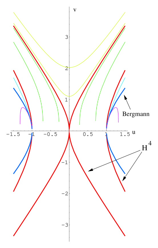
Figure 2: The phase plane for the first-order system of equation (83). The heavy blue hyperbola corresponds to the Bergmann flow, and the three heavy red hyperbolae to $H^{4}$ flows. The discussion of other flows is analogous to that for $\Lambda>0$; some representative examples are depicted.

4.6 Superpotential for the biaxial system

Although the $D=4$ self-dual Einstein spaces do not themselves have special holonomy, the existence of the first-order system implies that it might be possible to derive it from a superpotential. To obtain such a superpotential, we first notice that the Hamiltonian of the cohomogeneity one Einstein space is given by $H=T+U$, where

$$T = {2a_{1}^{\prime}\,a_{2}^{\prime}\over a_{1}\,a_{2}}+{2a_{1}^{\prime}\,a_{3}^{\prime}\over a_{1}\,a_{3}}+{2a_{2}^{\prime}\,a_{3}^{\prime}\over a_{2}\,a_{3}}\,,$$

$$U = {\textstyle{{\scriptstyle 1}\over{\scriptstyle 2}}}(a_{1}^{4}+a_{2}^{4}+a_{3}^{4}-2a_{1}^{2}\,a_{2}^{2}-2a_{1}^{2}\,a_{3}^{2}-2a_{2}^{2}\,a_{3}^{2}+12\lambda\,a_{1}^{2}\,a_{2}^{2}\,a^{2}_{3})\,,$$ (89)

and a prime denotes a derivative with respect to $\eta$ defined by $dt=a_{1}\,a_{2}\,a_{3}\,d\eta$.

Here, we shall consider the biaxial system with $a_{2}=a_{1}$, and use the $u$ and $a_{1}$ variables defined in section 4.2. We can write $T={\textstyle{{\scriptstyle 1}\over{\scriptstyle 2}}}g_{ij}\,(d\alpha^{i}/d\eta)\,(d\alpha^{j}/d\eta)$, with $\alpha_{i}=(a_{1},u)$, which implies that $g_{ij}$ is given by

$$g_{ij} = \pmatrix{{4x\over a_{1}^{2}y}&{4z\over a_{1}\,u\,y}\cr{4z\over a_{1}\,u\,y}&0\cr}\,,$$

$$x \equiv 1+3\lambda\,a_{1}^{2}-u^{2}\,,\quad y\equiv-1+\lambda\,a_{1}^{2}+u^{2}\,,\quad z\equiv-1+\lambda\,a_{1}^{2}+3u^{2}\,.$$ (90)

We find that the potential $U$ can then expressed as $U=-{\textstyle{{\scriptstyle 1}\over{\scriptstyle 2}}}g^{ij}\,(\partial W/\partial\alpha_{i})\,(\partial W/\partial\alpha_{j})$, with the superpotential $W$ given by

$$W=-{u^{2}\,(u^{2}-1)^{2}\over\lambda^{2}\,a_{1}^{2}}-{u^{2}\,(5u^{2}-4)\over\lambda}-a_{1}^{2}\,(3u^{2}+2)+\lambda\,a_{1}^{4}\,.$$ (91)

It is straightforward to derive the first order equations from this superpotential.

5 Triaxial anti-self-dual Bianchi IX metrics

In this section we discuss the full triaxial system of equations, which are considerably more complicated than the biaxial case.

5.1 Phase-plane and superpotential for triaxial system

We begin with an outline of a phase-plane analysis for the triaxial system, using methods similar to those that we used for the biaxial case.

Starting from the first-order equation for $\dot{a}_{1}$ obtained in (36), it is natural to define the auxiliary variable $w$, by

$$w\equiv\dot{a}_{1}-{a_{1}^{2}-a_{2}^{2}-a_{3}^{2}\over 2a_{2}\,a_{3}}\,.$$ (92)

In terms of $w$, equation (36) becomes

$$(w^{2}-1)^{2}\,(w-\lambda\,a_{2}\,a_{3})-\lambda^{2}\,a_{1}^{2}\,(a_{2}\,w+a_{3})(a_{3}\,w+a_{2})=0\,.$$ (93)

The remaining first-order equations in (30), namely those for $\dot{a}_{2}$ and $\dot{a}_{3}$, then become

$$\dot{a}_{2} = {a_{2}^{2}-a_{1}^{2}-a_{3}^{2}\over 2a_{1}\,a_{3}}-{\lambda\,a_{1}\,(a_{2}\,w+a_{3})\over w^{2}-1}\,,$$

$$\dot{a}_{3} = {a_{3}^{2}-a_{1}^{2}-a_{2}^{2}\over 2a_{1}\,a_{2}}-{\lambda\,a_{1}\,(a_{3}\,w+a_{2})\over w^{2}-1}\,.$$ (94)

We can now try following the strategy of treating $(w,a_{2},a_{3})$ as the independent variables, instead of $(a_{1},a_{2},a_{3})$. This is similar to the strategy used in the biaxial case, although not exactly parallel. Differentiating (93), using (94) and (92), and then using (93) itself to substitute for $a_{1}^{2}$, we get

$$(\dot{w}+\lambda\,a_{1})(w^{2}-1)^{2}\,[a_{2}\,a_{3}\,(3w^{4}+6w^{2}-1)-4(a_{2}^{2}+a_{3}^{2})\,w^{3}$$

$$\qquad\qquad\qquad-\lambda\,a_{2}\,a_{3}\,((a_{2}^{2}+a_{3}^{2})(1+3w^{2})+2a_{2}\,a_{3}\,w\,(w^{2}+3))]=0\,.$$ (95)

Unless the algebraic expression contained in square brackets vanishes, we therefore have the first-order equation

$$\dot{w}=-\lambda\,a_{1}\,.$$ (96)

We should think of $a_{1}$ as being solved for here, using (93). Since this would involve the use of square roots, it seems preferable to introduce a new radial variable $\rho$, defined by $d\rho=-a_{1}\,dt$. We then have

$$w^{\prime}=\lambda\,.$$ (97)

The remaining first-order equations (94) will also involve $a_{1}$ only through $a_{1}^{2}$, and so we shall have the system

$$w^{\prime} = \lambda\,,$$

$$a_{2}^{\prime} = -{a_{2}^{2}-a_{1}^{2}-a_{3}^{2}\over 2a_{1}^{2}\,a_{3}}+{\lambda\,(a_{2}\,w+a_{3})\over w^{2}-1}\,,$$

$$a_{3}^{\prime} = -{a_{3}^{2}-a_{1}^{2}-a_{2}^{2}\over 2a_{1}^{2}\,a_{2}}+{\lambda\,(a_{3}\,w+a_{2})\over w^{2}-1}\,,$$ (98)

where from (93), $a_{1}^{2}$ is given by

$$a_{1}^{2}={(w^{2}-1)^{2}\,(w-\lambda\,a_{2}\,a_{3})\over\lambda^{2}\,(a_{2}\,w+a_{3})(a_{3}\,w+a_{2})}\,.$$ (99)

Analogously to the biaxial case, we see from (93) that when $\lambda=0$ we have $w=0$ corresponding to the “BGPP” first-order equations, and $w=\pm 1$ corresponding to the “Atiyah-Hitchin” first-order equations.

The problem of solving the general triaxial first-order equations can be reduced to a second-order equation in a single variable. Defining $y\equiv a_{2}/a_{3}$ and $z\equiv a_{2}\,a_{3}$, we find, after normalising so that $\lambda=1$, that $y$ satisfies the equation

$$y^{\prime\prime}-{3y^{2}-2\rho\,y+1\over y\,(y^{2}-1)}\,{y^{\prime}}^{2}-{2\rho\,y^{2}-3\rho^{2}\,y-y+2\rho\over\rho\,(\rho^{2}-1)\,y}\,y^{\prime}+{2(y^{2}-1)\over\rho\,(\rho^{2}-1)^{2}}=0\,,$$ (100)

and that $z$ is given by

$$z={\rho\,(\rho^{2}-1)\,y\,[(\rho^{2}-1)\,y^{\prime}+1-y^{2}]\over(\rho^{2}-1)^{2}\,y\,y^{\prime}+\rho\,(y^{4}-1)+2y^{2}\,(y^{2}-1)}\,.$$ (101)

We find that it is possible to derive the triaxial first-order system from a superpotential also. We use $\alpha_{i}=(u,a_{2},a_{3})$ as variables, as discussed above. The kinetic energy $T$ given in (89) can be straightforwardly rewritten in terms of derivatives of $(u,a_{2},a_{3})$, and hence we can read off the components of the sigma-model metric $g_{ij}$ in $T={\textstyle{{\scriptstyle 1}\over{\scriptstyle 2}}}g_{ij}\,(d\alpha^{i}/d\eta)\,(d\alpha^{j}/d\eta)$, where as before $dt=a_{1}\,a_{2}\,a_{3}\,d\eta$. Since the expression for $g_{ij}$ is quite complicated, we shall not present it here. Then, we find after some calculation that the potential $U$ given in (89) can be written in terms of a superpotential $W$ as $U=-{\textstyle{{\scriptstyle 1}\over{\scriptstyle 2}}}g^{ij}\,(\partial W/\partial\alpha^{i})\,(\partial W/\partial\alpha^{j})$, with

$$W=-a_{2}^{2}-a_{3}^{2}-2\lambda^{-1}\,w^{2}+{a_{2}\,a_{3}\,(3w^{2}-1)\over w}+{(\lambda^{2}\,a_{2}^{2}\,a_{3}^{2}-w^{2})(w^{2}-1)^{2}\over\lambda^{2}\,w\,(a_{2}\,w+a_{3})(a_{3}\,w+a_{2})}\,.$$ (102)

It is easily verified that if one sets $a_{2}=a_{1}$, then $w$ reduces to the function $u$ of the biaxial system, and, after using (60) to replace $a_{3}$ by $u$, then $W+\lambda^{-1}$ becomes the biaxial superpotential given in (91), where $W$ denotes the triaxial superpotential (102) after the biaxial specialisations.

5.2 The Tod-Hitchin first-order system

In this section we shall follow Tod [27] and Hitchin [28, 29], who use a different approach to study the general triaxial system (30). The metric is written as

$$ds_{4}^{2}=F\,\Big{(}{dx^{2}\over x\,(1-x)}+{\sigma_{1}^{2}\over\Omega_{1}^{2}}+{(1-x)\,\sigma_{2}^{2}\over\Omega_{2}^{2}}+{x\,\sigma_{3}^{2}\over\Omega_{3}^{2}}\Big{)}\,.$$ (103)

Tod [27] shows that $ds_{4}^{2}$ is Einstein with anti-self-dual Weyl tensor if the functions $\Omega_{i}$ satisfy

$$\Omega_{1}^{\prime}=-{\Omega_{2}\,\Omega_{3}\over x\,(1-x)}\,,\quad\Omega_{2}^{\prime}=-{\Omega_{3}\,\Omega_{1}\over x}\,,\quad\Omega_{3}^{\prime}=-{\Omega_{1}\,\Omega_{2}\over 1-x}\,,$$ (104)

where a prime denotes a derivative with respect to $x$, and $F$ is given by

$$F=-{8x\,\Omega_{1}^{2}\,\Omega_{2}^{2}\,\Omega_{3}^{2}+2\Omega_{1}\,\Omega_{2}\,\Omega_{3}\,[x\,(\Omega_{1}^{2}+\Omega_{2}^{2})-(1-4\Omega_{3}^{2})(\Omega_{2}^{2}-(1-x)\,\Omega_{1}^{2})]\over 4(x\,\Omega_{1}\,\Omega_{2}+2\Omega_{3}\,(\Omega_{2}^{2}-(1-x)\,\Omega_{1}^{2}))^{2}}\,.$$ (105)

(We have normalised the Einstein constant so that $R_{ab}=3g_{ab}$.)

This first-order system can be reduced to the problem of solving the Painlevé VI equation [27]. One introduces a function $y(x)$, in terms of which the $\Omega_{i}^{2}$ are written as

$$\Omega_{1}^{2} = {(y-x)^{2}\,y\,(y-1)\over x\,(1-x)}\,\Big{(}z-{1\over 2(y-1)}\Big{)}\,\Big{(}z-{1\over 2y}\Big{)}\,,$$

$$\Omega_{2}^{2} = {y^{2}\,(y-1)(y-x)\over x}\,\Big{(}z-{1\over 2(y-x)}\Big{)}\,\Big{(}z-{1\over 2(y-1)}\Big{)}\,,$$ (106)

$$\Omega_{3}^{2} = {(y-1)^{2}\,y\,(y-x)\over(1-x)}\,\Big{(}z-{1\over 2y}\Big{)}\,\Big{(}z-{1\over 2(y-x)}\Big{)}\,,$$

where

$$z={x-2x\,y+y^{2}-2x\,(1-x)\,y^{\prime}\over 4y\,(y-1)(y-x)}\,.$$ (107)

(Note that $\Omega_{1}^{2}-\Omega_{2}^{2}-\Omega_{3}^{2}$, which is conserved, must take the value $-{\textstyle{{\scriptstyle 1}\over{\scriptstyle 4}}}$ in order that $ds_{4}^{2}$ be Einstein.) The claim then is that the first-order equations are satisfied if $y$ satisfies the Painlevé VI equation

$$y^{\prime\prime} = {\textstyle{{\scriptstyle 1}\over{\scriptstyle 2}}}\Big{(}{1\over y}+{1\over y-1}+{1\over y-x}\Big{)}\,{y^{\prime}}^{2}-\Big{(}{1\over x}+{1\over x-1}+{1\over y-x}\Big{)}\,y^{\prime}$$ (108)

$$+{y\,(y-1)(y-x)\over x^{2}\,(x-1)^{2}}\,\Big{(}\alpha+\beta\,{x\over y^{2}}+\gamma\,{x-1\over(y-1)^{2}}+\delta\,{x\,(x-1)\over(y-x)^{2}}\Big{)}\,,$$

with $(\alpha,\beta,\gamma,\delta)=({\textstyle{{\scriptstyle 1}\over{\scriptstyle 8}}},-{\textstyle{{\scriptstyle 1}\over{\scriptstyle 8}}},{\textstyle{{\scriptstyle 1}\over{\scriptstyle 8}}},{\textstyle{{\scriptstyle 3}\over{\scriptstyle 8}}})$. Note that the expression (105) for $F$ is actually quite simple, expressed in terms of $y$:

$$F = {y\,(1-y)\,(y-x)\,z\over 2x\,(1-x)}$$ (109)

$$= {x-2x\,y+y^{2}-2x\,(1-x)\,y^{\prime}\over 8x\,(1-x)}\,.$$

It is a straightforward, although somewhat involved, exercise to show that if the first-order equations (104) are satisfied, then the metric functions $a_{i}$ indeed satisfy our first-order equations (30). Note, however, that the converse is not true; not every solution of the general first-order equations (30) for anti-self-dual Einstein metrics gives a solution of (104). For example, the uniaxial solutions certainly do not satisfy the equations (104); setting the $a_{i}^{2}$ equal implies that $\Omega_{2}^{2}=(1-x)\,\Omega_{1}^{2}$ and $\Omega_{3}^{2}=x\,\Omega_{1}^{2}$, and one can easily see that substituting into (104) leads to a contradiction. Likewise, one can show that setting any two of the metric functions equal leads to a degeneration in (104). This can be understood from the fact that the radial coordinate used in [27, 28] becomes a constant if any two of the metric functions are set equal.

The first-order equations (104) were obtained in [27, 28, 29] by first solving the conditions for metrics with anti-self-dual Weyl tensor and vanishing Ricci scalar, and then performing a conformal rescaling of the metric to arrive at one that was Einstein. We have shown that every solution of the Tod-Hitchin system provides a solution of our system of first-order equations. Our equations are valid not only for the triaxial case but also for the biaxial and uniaxial cases, and yield all possible Bianchi IX self-dual Einstein metrics. The method of Tod and Hitchin breaks down in the biaxial and uniaxial cases. The arguments from twistor theory presented in [29] show that the Tod-Hitchin method gives the general triaxial metric, but the explicit correspondence to our first-order equations remains unclear.

5.3 Explicit examples

Hitchin gives explicit solutions to (108) characterised by an integer $k$, with $k=3,4,6,8$ [28, 29]. The case $k=3$ corresponds to the round metric on $S^{4}$, written in triaxial form [38], whilst $k=4$ corresponds to the Fubini-Study metric on ${{\mathbb{C}}{\mathbb{P}}}^{2}$, again written in triaxial form [44]. For $k\geq 5$ the metrics will necessarily have orbifold-type singularities.

In general it is easiest to give these solutions $y(x)$ by introducing a “parametric variable” $r$, with $y$ and $x$ both expressed in terms of $r$. Thus one has:

$$k=3: y={r^{2}\,(2r^{2}+5r+2)\over(2r+1)(r^{2}+r+1)}\,,\qquad x={r^{3}\,(r+2)\over 2r+1}\,,$$

$$k=4: y=r\,,\qquad x=r^{2}\,,$$

$$k=6: y={r\,(r^{2}+r+1)\over(2r+1)}\,,\qquad x={r^{3}\,(r+2)\over(2r+1)}\,,$$

$$k=8: {4r\,(3r^{2}-2r+1)\over(r+1)(1-r)^{3}\,(r^{2}+2r+3)}\,,\qquad x=\Big{(}{2r\over 1-r^{2}}\Big{)}^{4}\,.$$ (110)

It is straightforward to verify that these expressions all satisfy the Painlevé equation (108).

For $k=3$, after normalising so that $R_{ab}=3g_{ab}$, the metric (103) becomes [28]

$$h^{2}={3\over(1+r+r^{2})^{2}}\,,\quad a_{1}^{2}=(1+2r)^{2}\,h^{2}\,,\quad a_{2}^{2}=(1-r^{2})^{2}\,h^{2}\,,\quad a_{3}^{2}=r^{2}\,(2+r)^{2}\,h^{2}\,.$$ (111)

Note that the radial variable $r$ being used here is precisely the parametric variable in (110). Defining a new radial variable $t$ by $r=-{\textstyle{{\scriptstyle 1}\over{\scriptstyle 2}}}+{\textstyle{{\scriptstyle\sqrt{3}}\over{\scriptstyle 2}}}\,\tan({\textstyle{{\scriptstyle 1}\over{\scriptstyle 2}}}\sqrt{3}\,t)$, the $k=3$ metric becomes

$$ds_{4}^{2}=dt^{2}+4\sin^{2}t\,\sigma_{1}^{2}+4\sin^{2}(t-{\textstyle{{\scriptstyle 2}\over{\scriptstyle 3}}}\pi)\,\sigma_{2}^{2}+4\sin^{2}(t+{\textstyle{{\scriptstyle 2}\over{\scriptstyle 3}}}\pi)\,\sigma_{3}^{2}\,,$$ (112)

which can be recognised as the triaxial form of the Einstein metric on $S^{4}$, discussed in [38].

For $k=4$, and normalising for convenience so that $R_{ab}=6g_{ab}$, the metric in [28] has

$$h^{2}={1\over 4r\,(1+r)^{2}}\,,\quad a_{1}^{2}={1\over 1+r}\,,\quad a_{2}^{2}={(1-r)^{2}\over(1+r)^{2}}\,,\quad a_{3}^{2}={r\over 1+r}\,.$$ (113)

Defining a new radial variable by $r=\tan^{2}t$, the $k=4$ metric becomes

$$ds_{4}^{2}=dt^{2}+\cos^{2}t\,\sigma_{1}^{2}+\cos^{2}2t\,\sigma_{2}^{2}+\sin^{2}t\,\sigma_{3}^{2}\,,$$ (114)

which can be recognised as the triaxial ${{\mathbb{C}}{\mathbb{P}}}^{2}$ metric [44], discussed in appendix B.

For $k=6$, the metric functions are given by

$$h^{2}={3(1+r+r^{2})\over r\,(r+2)^{2}\,(2r+1)^{2}}\,,\qquad a_{1}^{2}={3(1+r+r^{2})\over(r+2)\,(2r+1)^{2}}\,,$$

$$a_{2}^{2}={3(r^{2}-1)^{2}\over(1+r+r^{2})\,(r+2)\,(2r+1)}\,,\qquad a_{3}^{2}={3r\,(1+r+r^{2})\over(r+2)^{2}\,(2r+1)}\,.$$ (115)

The radial coordinate runs from $r=1$ to $r=\infty$, and we have normalised the metric so that $R_{ab}=3g_{ab}$.

For $k=8$, after rederiving the metric using the construction given in [28], we find that the metric functions are given by

$$h^{2} = {4(1+r)(3-2r+r^{2})(1-2r+3r^{2})(1+2r+3r^{2})\over(1-r)\,r\,(1+r^{2})(1+2r-r^{2})^{2}\,(3+2r+r^{2})^{2}}\,,$$

$$a_{1}^{2} = {4(1-r)(1+r)^{3}\,(3-2r+r^{2})(1-2r+3r^{2})\over(1+2r-r^{2})(3+2r+r^{2})^{2}\,(1+2r+3r^{2})}\,,$$

$$a_{2}^{2} = {4(1+r^{2})(3-2r+r^{2})(1-2r-r^{2})^{2}\,(1+2r+3r^{2})\over(1+2r-r^{2})^{2}\,(3+2r+r^{2})^{2}\,(1-2r+3r^{2})}\,,$$

$$a_{3}^{2} = {16r\,(1-2r+3r^{2})(1+2r+3r^{2})\over(1+2r-r^{2})(3-2r+r^{2})(3+2r+r^{2})^{2}}\,,$$ (116)

where we have again chosen the normalisation so that $R_{ab}=3g_{ab}$. (This corrects a typographical error in [28], where there is an extra factor $(1+r)^{2}$ in the coefficient of $\sigma_{3}^{2}$ that should not be there.) The radial coordinate lies in the interval $\sqrt{2}-1<r<1$.

The $k=3$ and $k=4$ Tod-Hitchin metrics are $S^{4}$ and ${{\mathbb{C}}{\mathbb{P}}}^{2}$ respectively, albeit in their less common triaxial forms. The existence of more than one Bianchi IX form is a consequence of the homogeneity of these metrics. The isometry algebra contains more than one $SU(2)$ subalgebra, and the orbits are different. The full set of homogeneous Einstein 4-manifolds is known, and from that list we deduce that this can only happen for self-dual Einstein metrics in the case of $S^{4}$ and ${{\mathbb{C}}{\mathbb{P}}}^{2}$. Thus for higher values of $k$, the Tod-Hitchin metrics and the biaxial Bianchi IX self-dual Einstein metrics form disjoint classes. An explicit demonstration of this for the $k=6$ and $k=8$ metrics can be given by computing the quantity $X^{3}/Y^{2}$, where $X$ and $Y$ are the quadratic and cubic Weyl tensor invariants defined in (46). We showed that any biaxial self-dual Einstein metric must satisfy $X^{3}/Y^{2}=1$ (see (45)), and an elementary calculation shows that whilst this is true for the $k=3$ and $k=4$ metrics, it does not hold for the $k=6$ and $k=8$ metrics.

5.4 Global structure of the metrics

The global structure of the Tod-Hitchin metrics is described in detail in [28, 29]. Here, we summarise the conclusions, presenting them in a way that is perhaps more readily accessible to physicists.

The key to understanding the global structure is to understand the nature of the degenerate orbits where metric coefficients vanish. An important feature of the metrics, for all $k$ including $k=3$ and $k=4$, is that at one end of the radial coordinate range the coefficient of $\sigma_{1}$ vanishes, while at the other end it is the coefficient of $\sigma_{2}$ that vanishes instead. This “slumping” is reminiscent of the metric behaviour in the Atiyah-Hitchin metric, where the coefficient of one of the $\sigma_{i}$ vanishes at short distance, while the coefficient of another of them stablises in the asymptotic region. In fact, as shown in [28], the Atiyah-Hitchin metric itself arises as the $k\longrightarrow\infty$ limit of the Tod-Hitchin metrics.

Because of the slumping, it is useful to introduce two different Euler-angle parameterisations of the left-invariant 1-forms, one adapted to the region where $\sigma_{1}$ collapses, and the other adapted to the region where $\sigma_{2}$ collapses. The procedure was described in [39], and elaborated somewhat in [40]. Here we shall present a brief summary of the description in [40], with labelling adapted to our present conventions.

Let us introduce Euler angles $(\theta,\phi,\psi)$ and $(\tilde{\theta},\tilde{\phi},\widetilde{\psi})$, such that

$$\sigma_{1}=d\psi+\cos\theta\,d\phi\,,\quad\sigma_{2}+{{\rm i}}\,\sigma_{3}=e^{{{\rm i}}\,\psi}\,(d\theta+{{\rm i}}\,\sin\theta\,d\phi)\,,$$ (117)

$$\sigma_{2}=d\widetilde{\psi}+\cos\tilde{\theta}\,d\tilde{\phi}\,,\quad\sigma_{3}+{{\rm i}}\,\sigma_{1}=e^{{{\rm i}}\,\widetilde{\psi}}\,(d\tilde{\theta}+{{\rm i}}\,\sin\tilde{\theta}\,d\tilde{\phi})\,.$$ (118)

We begin by taking $\psi$ and $\widetilde{\psi}$ both to have period $2\pi$, so that the orbits are ${{\mathbb{R}}{\mathbb{P}}}^{3}$. Clearly one could, in principle, solve for the transformation that relates the tilded and untilded coordinates, but we shall not need this.

We now consider the operation, which we shall denote by $I_{1}$, which implements the identification $\psi\approx\psi+\pi$. It is easily seen that in terms of the tilded coordinates, this corresponds to $\tilde{\theta}\longrightarrow\pi-\tilde{\theta}$, $\tilde{\phi}\longrightarrow\tilde{\phi}+\pi$, $\widetilde{\psi}\longrightarrow-\widetilde{\psi}$. Likewise we define $\widetilde{I}_{2}$ which implements $\widetilde{\psi}\approx\widetilde{\psi}+\pi$. Since the tilded basis is related to the untilded by a cyclic permutation of $(\sigma_{1},\sigma_{2},\sigma_{3})$, we can see that in our notation we shall have $I_{i}=\widetilde{I}_{i}$, and so we can deduce that the effect of the $I_{i}$ on the untilded coordinates is

$$I_{1}: \theta\longrightarrow\theta\,,\qquad\phi\longrightarrow\phi\,,\qquad\psi\longrightarrow\psi+\pi\,,$$

$$I_{2}: \theta\longrightarrow\pi-\theta\,,\qquad\phi\longrightarrow\phi+\pi\,,\qquad\psi\longrightarrow-\psi\,,$$ (119)

$$I_{3}: \theta\longrightarrow\pi-\theta\,,\qquad\phi\longrightarrow\phi+\pi\,,\qquad\psi\longrightarrow\pi-\psi\,,$$

while on the tilded coordinates we have

$$I_{1}: \tilde{\theta}\longrightarrow\pi-\tilde{\theta}\,,\qquad\tilde{\phi}\longrightarrow\tilde{\phi}+\pi\,,\qquad\widetilde{\psi}\longrightarrow\pi-\widetilde{\psi}\,,$$

$$I_{2}: \tilde{\theta}\longrightarrow\tilde{\theta}\,,\qquad\tilde{\phi}\longrightarrow\tilde{\phi}\,,\qquad\widetilde{\psi}\longrightarrow\widetilde{\psi}+\pi\,,$$ (120)

$$I_{3}: \tilde{\theta}\longrightarrow\pi-\tilde{\theta}\,,\qquad\tilde{\phi}\longrightarrow\tilde{\phi}+\pi\,,\qquad\widetilde{\psi}\longrightarrow-\widetilde{\psi}\,,$$

Consider first the case $k=3$, which gives the triaxial metric (112) on $S^{4}$. Near $t=0$ we have

$$ds_{4}^{2}\sim dt^{2}+4t^{2}\,\sigma_{1}^{2}+\sigma_{2}^{2}+\sigma_{3}^{2}\,.$$ (121)

From the expression (117) we see that regularity at $t=0$ requires that $\psi$ have period $\pi$, and so from (119) we should impose the identification $I_{1}$. Near the other endpoint $t={\textstyle{{\scriptstyle 2}\over{\scriptstyle 3}}}\pi$, we set $t={\textstyle{{\scriptstyle 2}\over{\scriptstyle 3}}}\pi-\tau$, and so the metric takes the form

$$ds_{4}^{2}\sim d\tau^{2}+4\tau^{2}\,\sigma_{2}^{2}+\sigma_{1}^{2}+\sigma_{3}^{2}\,.$$ (122)

From (118) we see that regularity requires that $\widetilde{\psi}$ have period $\pi$, and so from (120) we should in addition impose the identification $I_{2}$. Thus the principal orbits are $SO(3)/({{\mathbb{Z}}}_{2}\times{{\mathbb{Z}}}_{2})$. We also see that the 2-dimensional bolt described by $\sigma_{2}^{2}+\sigma_{3}^{2}=d\theta^{2}+\sin^{2}\theta\,d\phi^{2}$ at $t=0$, and the 2-dimensional bolt described by $\sigma_{1}^{2}+\sigma_{3}^{2}=d\tilde{\theta}^{2}+\sin^{2}\tilde{\theta}\,d\tilde{\phi}^{2}$ at $t={\textstyle{{\scriptstyle 2}\over{\scriptstyle 3}}}\pi$ each has the topology of ${{\mathbb{R}}{\mathbb{P}}}^{2}$, since there is an antipodal identification on the former implied by $I_{2}$ in (119), and in the latter implied by $I_{1}$ in (120). The metric therefore extends smoothly on the Veronese surfaces ${{\mathbb{R}}{\mathbb{P}}}^{2}$ at each endpoint [28].

The case $k=4$ gives the triaxial ${{\mathbb{C}}{\mathbb{P}}}^{2}$ metric (114). We can take the two endpoints to be at $t={\textstyle{{\scriptstyle 1}\over{\scriptstyle 2}}}\pi$ and $t={\textstyle{{\scriptstyle 1}\over{\scriptstyle 4}}}\pi$. Near $t={\textstyle{{\scriptstyle 1}\over{\scriptstyle 2}}}\pi$, after setting $t={\textstyle{{\scriptstyle 1}\over{\scriptstyle 2}}}\pi-\tau$ the metric takes the form

$$ds_{4}^{2}\sim d\tau^{2}+\tau^{2}\,\sigma_{1}^{2}+\sigma_{2}^{2}+\sigma_{3}^{2}\,.$$ (123)

Regularity therefore requires that we not impose the identification $I_{1}$. On the other hand, at the other endpoint $t={\textstyle{{\scriptstyle 1}\over{\scriptstyle 4}}}\pi$, after defining $t={\textstyle{{\scriptstyle 1}\over{\scriptstyle 4}}}\pi-\tau$ we have

$$ds_{4}^{2}\sim d\tau^{2}+4\tau^{2}\,\sigma_{2}^{2}+\sigma_{1}^{2}+\sigma_{3}^{2}\,.$$ (124)

Regularity therefore requires that we impose the identification $I_{2}$. This means that the principal orbits are $SO(3)/{{\mathbb{Z}}}_{2}$, and that the metric extends smoothly onto ${{\mathbb{R}}{\mathbb{P}}}^{2}$ at $t={\textstyle{{\scriptstyle 1}\over{\scriptstyle 2}}}\pi$, and onto $S^{2}$ at $t={\textstyle{{\scriptstyle 1}\over{\scriptstyle 4}}}\pi$ [28]. This reflects the fact that ${{\mathbb{C}}{\mathbb{P}}}^{2}$ can be described as the double covering of $S^{4}$ branched over ${{\mathbb{R}}{\mathbb{P}}}^{2}$.

For $k=6$, we see by letting $r=1+3\rho$ that near $r=1$ the metric (115) takes the form

$$ds_{4}^{2}\sim d\rho^{2}+4\rho^{2}\,\sigma_{2}^{2}+{\textstyle{{\scriptstyle 1}\over{\scriptstyle 3}}}(\sigma_{1}^{2}+\sigma_{3}^{2})\,,$$ (125)

whilst letting $r=1/\rho^{2}$ the metric near $r=\infty$ has the form

$$ds_{4}^{2}\sim d\rho^{2}+{\textstyle{{\scriptstyle 1}\over{\scriptstyle 4}}}\rho^{2}\,\sigma_{1}^{2}+{\textstyle{{\scriptstyle 3}\over{\scriptstyle 2}}}(\sigma_{2}^{2}+\sigma_{3}^{2})\,.$$ (126)

Thus if we impose the identification $I_{2}$ the metric extends smoothly over ${{\mathbb{R}}{\mathbb{P}}}^{2}$ at $r=1$, and extends over ${{\mathbb{R}}{\mathbb{P}}}^{2}$ with an orbifold singularity having angle ${\textstyle{{\scriptstyle 1}\over{\scriptstyle 2}}}\pi$ at $r=\infty$ [28].

For $k=8$, after letting $r=\sqrt{2}-1+(\sqrt{2-\sqrt{2}})\,\rho$, the metric near $r=\sqrt{2}-1$ can be seen to have the form

$$ds_{4}^{2}\sim d\rho^{2}+4\rho^{2}\,\sigma_{2}^{2}+(3-2\sqrt{2})\,(\sigma_{1}^{2}+\sigma_{3}^{2})\,.$$ (127)

Letting $r=1-{\textstyle{{\scriptstyle 3}\over{\scriptstyle 8}}}\rho^{2}$, the metric near $r=1$ takes the form

$$ds_{4}^{2}\sim d\rho^{2}+{\textstyle{{\scriptstyle 1}\over{\scriptstyle 9}}}\rho^{2}\,\sigma_{1}^{2}+{\textstyle{{\scriptstyle 4}\over{\scriptstyle 3}}}(\sigma_{2}^{2}+\sigma_{3}^{2})\,.$$ (128)

Thus by imposing the identification $I_{2}$ the metric extends smoothly over ${{\mathbb{R}}{\mathbb{P}}}^{2}$ at $r=\sqrt{2}-1$, and extends over ${{\mathbb{R}}{\mathbb{P}}}^{2}$ with an orbifold singularity having angle ${\textstyle{{\scriptstyle 1}\over{\scriptstyle 3}}}\pi$ at $r=1$ [28].

In [28] it is shown that all the metrics obtained from solving the Painlevé equation are positive definite with $x$ lying in the interval $1<x<\infty$, for all values of the constant $k$ parameterising the solutions described in [28]. Near $x=1$, the metric takes the form

$$ds_{4}^{2}\sim{\textstyle{{\scriptstyle 1}\over{\scriptstyle 16}}}\cos^{2}{\pi\over k}\,(dr^{2}+4r^{2}\,\sigma_{2}^{2})+\sigma_{1}^{2}+\sigma_{3}^{2}\,.$$ (129)

This shows that the metric extends over the degenerate orbit at $r=0$, with $\sigma_{1}^{2}+\sigma_{3}^{2}$ describing ${{\mathbb{R}}{\mathbb{P}}}^{2}$ [28]. As $x\longrightarrow\infty$ the metric assumes the form

$$ds_{4}^{2}\sim d\rho^{2}+{4\rho^{2}\over(k-2)^{2}}\,\sigma_{1}^{2}+2^{8/k-2}\,(\sigma_{2}^{2}+\sigma_{3}^{2})\,,$$ (130)

where $x=\rho^{-k}$, which shows that there is an orbifold singularity with angle $2\pi/(k-2)$ around ${{\mathbb{R}}{\mathbb{P}}}^{2}$ [28]. These results are consistent with the explicit calculations for the $k=6$ and $k=8$ cases above.

6 Singularity structure and M-theory

In this paper we have extended the analysis of $G_{2}$ holonomy spaces to those whose principal orbits are twistor spaces, constructed as $S^{2}$ bundles over four-dimensional self-dual Einstein metrics of the general Bianchi IX type. We obtained the general first-order differential equations for these triaxial Bianchi IX metrics, and we showed how they can be derived from a superpotential. In special cases, the self-dual Einstein metrics reduce to $S^{4}$, ${{\mathbb{C}}{\mathbb{P}}}^{2}$ and the (biaxial) Taub-NUT-de Sitter metrics,

We focused on the analysis of the local and global structures of the self-dual Einstein Bianchi IX metrics. For the biaxial specialisation, where the local form of the general solution is well known, we gave a complete analysis of the solutions by studying the flows in the phase-plane of the first-order equations. Even in this biaxial case the analysis is quite subtle, since there is no single local expression for the metric that directly covers all the possible regions of flows in the phase-plane. Some regions are well-described by the standard expression for the self-dual Taub-NUT-de Sitter metrics, but our analysis reveals that in another region there are flows that are more appropriately described by a different local form of the solution, which we refer to as the self-dual Eguchi-Hanson-de Sitter metrics. These metrics, which as far as we are aware have not been presented explicitly before, describe flows in a region of the phase-plane that can be viewed as generalisations of the Eguchi-Hanson metric in which the cosmological constant is non-zero. Unlike the usual Eguchi-Hanson-de Sitter metrics [37], which are Kähler but neither self-dual nor anti-self-dual, the new metrics have a self-dual Weyl tensor even when the cosmological constant is non-zero. In the self-dual Taub-NUT-de Sitter form, the two parameters of biaxial solutions can be thought of as the NUT parameter and the cosmological constant. In the self-dual Eguchi-Hanson-de Sitter form, the two parameters can be thought of as the Eguchi-Hanson scale size and the cosmological constant.

We discussed the global structure for the biaxial self-dual metrics, both for positive and negative cosmological constant. For the positive cosmological constant the metrics are compact, in general with singularities. The radial coordinate ranges over an interval that terminates at endpoints where the $SU(2)$ principal orbits degenerate; to a point (a NUT) at one end, and to a two-dimensional surface (a bolt) that is (locally) $S^{2}$ at the other. For generic choices of the NUT parameter (or, in the alternative local description, the Eguchi-Hanson scale size), the metrics cannot be smoothly extended on the NUT and bolt endpoints simultaneously. This is because the periodicity requirements needed for regularity at one end are in general incommensurate with the periodicity requirements at the other end. Only for very special values of the NUT parameter is the metric regular at both endpoints. In general, however, one encounters singularities at either endpoint of the four-dimensional radial coordinate.

In the generic case, a specific choice of the period for the azimuthal angle $\psi$ allows the singularity at the $S^{2}$ bolt to be removed, but then the NUT has a co-dimension four orbifold singularity. Alternatively, choosing the periodicity appropriate for regularity at the NUT, there will be a co-dimension two singularity on the $S^{2}$ bolt. The associated seven-dimensional $G_{2}$ holonomy space therefore has singularities of the same co-dimensions. The co-dimension four NUT singularities may admit an M-theory interpretation associated with the appearance of non-abelian gauge symmetries [16] and the circle reduction of M-theory on these $G_{2}$ holonomy spaces may have a Type IIA interpretation in terms of a location of coincident D6-branes [16]. On the other hand the co-dimension two singularities at the bolts do not seem to have a straightforward interpretation in M-theory dynamics. Since neither of type of singularity is of co-dimension seven, these spaces do not seem to shed light on the appearance of chiral matter.

The triaxial self-dual Einstein Bianchi IX metrics described by the Tod-Hitchin system are defined on compact spaces with bolts at each endpoint. For the solutions discussed in section 5.3, with $k\geq 6$, one endpoint has an ${{\mathbb{R}}{\mathbb{P}}}^{2}$ bolt, while the other endpoint is a ${{\mathbb{R}}{\mathbb{P}}}^{2}$ bolt with a ${{\mathbb{Z}}}_{k-2}$ conical co-dimension two singularity. The corresponding $G_{2}$ holonomy spaces again have co-dimension two singularities, and so M-theory on these spaces does not have a straightforward interpretation; in particular their relevance for obtaining non-abelian gauge group enhancement or the appearance of chiral matter is not clear.

Despite the fact that the role of the singularities in our metrics in M-theory is unclear, one thing is certain: the singularities do not affect the amount of supersymmetry. Because the Killing spinor is a singlet, it is invariant under all elements of the isometry group. In particular, it is invariant under the action of the binary dihedral group generated by $I_{1}$, $I_{2}$ and $I_{3}$, and in the biaxial case it is invariant under arbitrary shifts of the coordinate $\psi$. Since it was these symmetries that entered into the discussion of singularities, it is clear that no matter what identifications we choose to make, it will not affect the existence of the Killing spinor. This should be contrasted with the co-dimension two and co-dimension four singularities discussed in [49]. In that case, the Killing spinors are not singlets, and identifications may or may not leave them invariant. The singularities for which the identifications are incompatible with the existence of Killing spinors are believed to be unstable, due to closed-string tachyons, whilst those that are compatible with the Killing spinors are believed to be stable. In our case, it is clear that there is no room for a closed-string tachyon instability, or its M-theoretic analogue. In other words, “Don’t Panic, it’s $G_{2}$!”

Appendix A Bianchi IX Einstein-Kähler metrics

The purpose of this appendix is to clarify the distinction between the anti-self-dual Einstein metrics considered in this paper and Bianchi IX Einstein-Kähler metrics. These two classes do not overlap except when the metrics are Ricci-flat, or else the Fubini-Study metric on ${{\mathbb{C}}{\mathbb{P}}}^{2}$ (or the Bergmann metric on the open ball in ${{\mathbb{C}}}^{2}$ if $\Lambda<0$). In the case that the metrics are biaxial, the general Einstein-Kähler solutions, together with their Kähler potential, were obtained in [37], where they were called the Eguchi-Hanson-de Sitter metrics (see equation (57)). A subsequent discussion was given in [42].

The triaxial case has been considered by Dancer and Strachan in [43], where a first-order system was obtained. This generalises that for hyper-Kähler metrics with triholomorphic $SU(2)$ action, written down and solved in [34]. The general solution of the Dancer-Strachan system is not known, but particular cases, such as triaxial forms of the Fubini-Study metric on ${{\mathbb{C}}{\mathbb{P}}}^{2}$ and the product metric on ${{\mathbb{C}}{\mathbb{P}}}^{1}\times{{\mathbb{C}}{\mathbb{P}}}^{1}$ are known, and turn out to be remarkably simple.

Writing the Bianchi IX metrics in the form (24), with $e^{0}=dt$ and $e^{i}=a_{i}\,\sigma_{i}$, a basis for anti-self-dual 2-forms is $\Omega_{i}=e^{0}\wedge e^{i}-{\textstyle{{\scriptstyle 1}\over{\scriptstyle 2}}}{\epsilon}_{ijk}\,\epsilon^{j}\wedge e^{k}$, and so an ansatz for the $SU(2)$-invariant anti-self-dual Kähler form is

$$\Omega=\alpha_{i}\,\Omega_{i}\,,$$ (131)

where the coefficients $\alpha_{i}$ depend only on $t$, and $\alpha_{i}^{2}=1$. The metric will be Kähler if $\Omega$ is covariantly constant, which leads to the first-order equations

$$\dot{\alpha}_{1}=(\beta_{3}+\gamma_{3})\,\alpha_{2}-(\beta_{2}+\gamma_{2})\,\alpha_{3}\,,\qquad{\hbox{and cyclic}}\,,$$ (132)

where $\beta_{i}$ and $\gamma_{i}$ are defined in (27). From these, and the Einstein equations, one can show that $\alpha_{1}=\alpha_{2}=0$ and $\alpha_{3}=1$ (or cyclic permutations) [43], and hence that the metric coefficients satisfy the first-order equations

$$\dot{a}_{1} = -{a_{1}^{2}-a_{2}^{2}-a_{3}^{2}\over 2a_{2}\,a_{3}}\,,$$

$$\dot{a}_{2} = -{a_{2}^{2}-a_{1}^{2}-a_{3}^{2}\over 2a_{1}\,a_{3}}\,,$$ (133)

$$\dot{a}_{3} = -{a_{3}^{2}-a_{1}^{2}-a_{2}^{2}+2\Lambda\,a_{1}^{2}\,a_{2}^{2}\over 2a_{1}\,a_{2}}\,,$$

Rewriting in terms of the radial variable $\eta$, defined by $dt=a_{1}\,a_{2}\,a_{3}\,d\eta$, it is easily seen that the first-order equations can be derived from a superpotential. In the notation of section 4.6, the potential $U$ in (89) can be written as $U=-{\textstyle{{\scriptstyle 1}\over{\scriptstyle 2}}}g^{ij}\,(\partial W/\partial\alpha^{i})\,(\partial W/\partial\alpha^{j})$, where we now define $\alpha^{i}=(\log a_{1},\log a_{2},\log a_{3})$, and hence $g_{ij}=2-2\delta_{ij}$. We find that the superpotential is then given by

$$W=-(a_{1}^{2}+a_{2}^{2}+a_{3}^{2})+\Lambda\,a_{1}^{2}\,a_{2}^{2}\,.$$ (134)

Two particular triaxial solutions of the first-order Einstein-Kähler system (133) are the Fubini-Study metric on ${{\mathbb{C}}{\mathbb{P}}}^{2}$, which can be written (setting $\Lambda=6$ for convenience) as [44]

$$ds_{4}^{2}=dt^{2}+\sin^{2}t\,\sigma_{1}^{2}+\cos^{2}t\,\sigma_{2}^{2}+\cos^{2}2t\,\sigma_{3}^{2}\,,$$ (135)

and the product metric on $S^{2}\times S^{2}$, which can be written (setting $\Lambda=2$ for convenience) as [45]

$$ds_{4}^{2}=dt^{2}+\sin^{2}t\,\sigma_{1}^{2}+\sigma_{2}^{2}+\cos^{2}t\,\sigma_{3}^{2}\,.$$ (136)

In view of the somewhat unfamiliar forms of these metrics, we shall give a brief description of them below.

Appendix B Iwai’s construction, Dragt coordinates and the Guichardet connection

In this appendix, we shall derive the triaxial forms of the Einstein metrics on ${{\mathbb{C}}{\mathbb{P}}}^{2}$ and $S^{2}\times S^{2}$. The method used differs slightly from the ones in [44] and [45], but it has the merit of giving a unified description of the two cases. The basic idea is to express the metric in flat Euclidean 6-space in an appropriate coordinate system, adapted to an $SO(3)$ action. We shall here follow the paper of Iwai [46], who was interested in the three-body problem in molecular physics. It turns out that we can use his results not only to obtain Bianchi IX metrics but we can also use Scherk-Schwarz reduction to obtain some insight into global monopoles of the sort recently studied by Hartnoll [47].

We think of ${{\mathbb{E}}}^{6}$ as ${{\mathbb{E}}}^{3}\oplus{{\mathbb{E}}}^{3}\ni({\bf x},{\bf y})$ and consider the diagonal action of $SO(3)$. Projection from the principal orbits is Iwai’s generalisation of the standard Hopf map used in the Taub-NUT metric. This standard Hopf map $\pi:{{\mathbb{E}}}^{4}\equiv({{\mathbb{C}}}\oplus{{\mathbb{C}}})\ni(z^{1},z^{2})\rightarrow{{\mathbb{R}}}^{3}\equiv{{\mathbb{R}}}\oplus{{\mathbb{C}}}$ onto the orbits of the diagonal action of $U(1)$ given by

$$(z^{1},z^{2})\rightarrow(|z^{1}|^{2}-|z^{2}|^{2},2z^{1}{\bar{z}^{2}})\,.$$ (137)

Introducing polar coordinates on ${{\mathbb{R}}}^{3}$, and an angle $\psi$ along the Hopf fibres, we may write the flat metric on ${{\mathbb{E}}}^{4}$ as a special case of the multi-centre metrics, which have an interpretation in terms Kaluza-Klein monopoles and D6-branes. Iwai’s procedure is rather similar and may have a corresponding generalisation.

In the case of flat six dimensions, Iwai’s map is $\pi:{{\mathbb{E}}}^{6}\rightarrow{{\mathbb{R}}}^{3}_{+}\ni(w^{1},w^{2},w^{3})$, given by

$$({\bf x},{\bf y})\rightarrow({\bf x}^{2}-{\bf y}^{2},2{\bf x}\cdot{\bf y},2|{\bf x}\times{\bf y}|)=(w^{1},w^{2},w^{3})\,,$$ (138)

with $w^{3}\geq 0$. Th orbit space ${{\mathbb{R}}}^{3}_{+}$ may be given coordinates $(\rho,\psi,\chi)$, called Dragt coordinates, such that

$$(w^{1},w^{2},w^{3})=(\rho^{2}\cos\psi\cos\chi,\rho^{2}\sin\psi\cos\chi,\rho^{2}\sin\chi)\,,$$ (139)

with $0\leq\rho<\infty$, $0\leq\psi<2\pi$, $0\leq\chi<{\pi\over 2}$. Note the range of $\chi$. One checks that

$${\bf x}^{2}+{\bf y}^{2}=\rho^{2}=\sqrt{(w^{1})^{2}+(w^{2})^{2}+(w^{3})^{2}}\,.$$ (140)

To fix the $SO(3)$ freedom we introduce an orthonormal moving frame $({\bf u}_{1},{\bf u}_{2},{\bf u}_{3})$ related to a fixed orthonormal frame $({\bf e}_{1},{\bf e}_{2},{\bf e}_{3})$ by a rotation with standard Euler angles and left-invariant 1-forms $(\sigma_{1},\sigma_{2},\sigma_{3})$ say. Now if

$${\bf x}=\rho\cos{\psi\over 2}\cos{\chi\over 2}{\bf u}_{1}-\rho\sin{\psi\over 2}\sin{\chi\over 2}{\bf u}_{2}\,,$$ (141)

and

$${\bf y}=\rho\sin{\psi\over 2}\cos{\chi\over 2}{\bf u}_{1}+\rho\cos{\psi\over 2}\sin{\chi\over 2}{\bf u}_{2}\,,$$ (142)

Iwai finds that the flat metric on ${{\mathbb{E}}}^{6}$ is given by

$$ds^{2}=d\rho^{2}+{\textstyle{{\scriptstyle 1}\over{\scriptstyle 4}}}\rho^{2}(d\chi^{2}+\cos^{2}\chi d\psi^{2})+\rho^{2}\sin^{2}{\chi\over 2}\,\sigma_{1}^{2}+\rho^{2}\cos^{2}{\chi\over 2}\,\sigma_{2}^{2}+\rho^{2}(\sigma_{3}-{\textstyle{{\scriptstyle 1}\over{\scriptstyle 2}}}\sin\chi\,d\psi)^{2}\,.$$ (143)

If we set $\psi={\textstyle{{\scriptstyle 1}\over{\scriptstyle 2}}}\pi$ and $\rho^{2}=2$, the vectors ${\bf x}$ and ${\bf y}$ have unit magnitudes, and thus parameterise points on $S^{2}\times S^{2}$, embedded in ${{\mathbb{R}}}^{3}\times{{\mathbb{R}}}^{3}$. The result is the metric (136) on $S^{2}\times S^{2}$, obtained in [45].

If instead we set $\rho=1$ we obtain the unit $S^{5}$. The angle $\psi$ is a coordinate along the Hopf fibres. Projecting orthogonally to the Hopf fibres, we obtain the triaxial form (135) of the Fubini-Study metric on ${{\mathbb{C}}{\mathbb{P}}}^{2}$ obtained in [44].

We note en passant that we could consider the seven-dimensional flat metric on ${{\mathbb{E}}}^{6,1}$ as a trivial solution of supergravity, and perform a Scherk-Schwarz reduction on the orbits of $SO(3)$. We get in four dimensions a global monopole coupled to an $SO(3)$ gauge field $A^{i}$, $i=1,2,3$, with the Higgs field in the symmetric tensor (i.e. the ${\bf 5}$) representation of $SO(3)$. The gauge connection coincides with the Guichardet connection, and in the present case the only non-zero gauge field is

$$A^{3}=-{\textstyle{{\scriptstyle 1}\over{\scriptstyle 2}}}\sin\chi\,d\psi\,.$$ (144)

Ignoring the Weyl rescaling, the interpretation is as follows. One should think of $\psi$ as an azimuthal angle, i.e. a longitude, while $\chi$ is to be thought of as a latitude. Because $\chi\in[0,{\pi\over 2})$, there is a deficit solid angle, and hence a conical singularity at the origin. Moreover, the metric is not asymptotically flat. We have an embedding of an abelian monopole into the non-abelian gauge group $SO(3)$. This monopole may be thought of as sitting at the centre of a global monopole supported by a Higgs field.

Appendix C Killing spinors

Since the seven-dimensional metric constructed from the anti-self-dual Einstein 4-metric according to (12) has $G_{2}$ holonomy, it follows that it admits a covariantly-constant spinor. It is instructive to look at how this is related to spinors in the four-dimensional base space. To do this, we begin by calculating the Lorentz-covariant exterior derivative on spinors in seven dimensions in terms of quantities in the four-dimensional base metric. We adopt a notation where quantities in seven dimensions carry hats, and so we write (12) as $d\hat{s}_{7}^{2}=\rho^{-1}\,(Du_{i})^{2}+2\rho\,ds_{4}^{2}$, for which we choose the natural vielbein basis $\hat{e}^{i}=\rho^{-1/2}\,Du_{i}$, $\hat{e}^{a}=\sqrt{2\rho}\,e^{a}$. The spinor-covariant exterior derivative is given by $\hat{\nabla}\equiv d+{\textstyle{{\scriptstyle 1}\over{\scriptstyle 4}}}\hat{\omega}_{AB}\,\hat{\Gamma}^{AB}$, and after some calculation we find that this is given by

$$\hat{\nabla} = d+{\textstyle{{\scriptstyle 1}\over{\scriptstyle 4}}}\omega_{ab}\,\hat{\Gamma}^{ab}-{\textstyle{{\scriptstyle 1}\over{\scriptstyle 4}}}{\epsilon}_{ijk}\,A^{k}\,\hat{\Gamma}^{ij}+{\textstyle{{\scriptstyle 1}\over{\scriptstyle 16}}}\rho^{-3/2}\,u_{j}\,({\epsilon}_{ijk}\,J^{k}_{ab}\,\hat{\Gamma}^{ab}-4\hat{\Gamma}^{ij})\,\hat{e}^{i}$$ (145)

$$+{\textstyle{{\scriptstyle 1}\over{\scriptstyle 8}}}\rho^{-3/2}\,u_{i}\,({\epsilon}_{ijk}\,J^{j}_{ab}\,\hat{\Gamma}^{kb}-2\hat{\Gamma}^{ia})\,\hat{e}^{a}\,.$$

The covariantly-constant spinor $\hat{\eta}$ in the seven-dimensional $G_{2}$ metric satisfies $\hat{\nabla}\,\hat{\eta}=0$. It can be seen from (145) that this spinor is annihilated by the terms involving the ${{\mathbb{R}}}^{3}$ coordinates $u_{i}$, and that it is independent of $u_{i}$. In fact in this basis we find that $\hat{\eta}$ is the spinor that is determined, up to overall $u_{i}$-independent scale, by the conditions

$$\hat{\Gamma}_{ij}\,\hat{\eta}={\textstyle{{\scriptstyle 1}\over{\scriptstyle 4}}}{\epsilon}_{ijk}\,J^{k}_{ab}\,\hat{\Gamma}_{ab}\,\hat{\eta}\,.$$ (146)

It then follows from (145) that $\hat{\eta}$ satisfies

$$(d+{\textstyle{{\scriptstyle 1}\over{\scriptstyle 4}}}\omega_{ab}\,\hat{\Gamma}^{ab}-{\textstyle{{\scriptstyle 1}\over{\scriptstyle 4}}}{\epsilon}_{ijk}\,A^{k}\,\hat{\Gamma}^{ij})\,\hat{\eta}=0\,.$$ (147)

Decomposing spinors into the tensor product of spinors in the four-dimensional base and the ${{\mathbb{R}}}^{3}$ fibres, we choose Dirac matrices $\hat{\Gamma}_{a}=\Gamma_{a}\otimes\hbox to0.0pt{1\hss}\mkern 4.0mu{\rm l}$ and $\hat{\Gamma}_{i}=\Gamma_{5}\otimes\tau_{i}$. The Pauli matrices $\tau_{i}$ can be viewed as the generators of an internal $SU(2)$ isospin, and so (146) and (147) can be written as

$$J^{i}_{ab}\,\Gamma^{ab}\,\eta^{\alpha}=4{{\rm i}}\,(\tau_{i})^{\alpha}{}_{\beta}\,\eta^{\beta}\,,\qquad\nabla\,\eta^{\alpha}-{\textstyle{{\scriptstyle{{\rm i}}}\over{\scriptstyle 4}}}A^{i}\,(\tau_{i})^{\alpha}{}_{\beta}\,\eta^{\beta}=0\,.$$ (148)

The second equation is the condition for the 4-component spinor $\eta^{\alpha}$ with its isospin doublet index $\alpha$ to be gauge covariantly constant with respect to the $SU(2)$ Yang-Mills covariant derivative.

Using (146) we can rewrite (147) as the four-dimensional equation

$$d\eta^{\alpha}+{\textstyle{{\scriptstyle 1}\over{\scriptstyle 4}}}(\omega_{ab}-{\textstyle{{\scriptstyle 1}\over{\scriptstyle 2}}}A^{i}\,J_{ab})\,\Gamma^{ab}\,\eta^{\alpha}=0\,.$$ (149)

With the Yang-Mills connection taken to be the self-dual part of the four-dimensional spin connection as in (25), we therefore find that (149) is nothing but

$$d\eta^{\alpha}+{\textstyle{{\scriptstyle 1}\over{\scriptstyle 4}}}\omega^{-}_{ab}\,\Gamma^{ab}\,\eta^{\alpha}=0\,,$$ (150)

where $\omega^{-}_{ab}\equiv{\textstyle{{\scriptstyle 1}\over{\scriptstyle 2}}}(\omega_{ab}-{\textstyle{{\scriptstyle 1}\over{\scriptstyle 2}}}{\epsilon}_{abcd}\,\omega^{cd})$ is the anti-self-dual part of the spin connection. In fact it follows from the conditions (146) satisfied by $\hat{\eta}$ that $\hat{\Gamma}_{ab}\,\hat{\eta}$ is self-dual in the four-dimensional base space, and hence (150) reduces simply to $d\eta^{\alpha}=0$.

It is interesting to note that in the special case of ${{\mathbb{C}}{\mathbb{P}}}^{2}$, which does not admit an ordinary sin structure, $\eta^{\alpha}$ is a generalised spinor (in the terminology of [48]) that is charged with respect to the Yang-Mills connection $A^{i}$. In this case the connection is actually $SO(3)$-valued, as opposed to $SU(2)$-valued, and it is this that serves to compensate for the minus sign that ordinary spinors would acquire upon parallel propagation around a family of curves spanning the bolt in ${{\mathbb{C}}{\mathbb{P}}}^{2}$ [48].

References

- [1]
- [2] R.L. Bryant and S. Salamon, On the construction of some complete metrics with exceptional holonomy, Duke Math. J. 58, 829 (1989).
- [3]
- [4] G.W. Gibbons, D.N. Page and C.N. Pope, Einstein metrics on , and bundles, Commun. Math. Phys. 127, 529 (1990).
- [5]
- [6] A.L. Besse, Einstein manifolds, Springer Verlag, Berlin-Heidelberg (1987).
- [7]
- [8] M. Cvetič, G. Shiu and A.M. Uranga, Three-family supersymmetric standard like models from intersecting brane worlds, Phys. Rev. Lett. 87, 201801 (2001), hep-th/0107143; Chiral four-dimensional N = 1 supersymmetric type IIA orientifolds from intersecting D6-branes, Nucl. Phys. B615, 3-32 (2001), hep-th/0107166.
- [9]
- [10] M.F. Atiyah and E. Witten, M-theory dynamics on a manifold of holonomy, hep-th/0107177.
- [11]
- [12] E. Witten, Anomaly cancellation on manifold, hep-th/0108165.
- [13] B. Acharya and E. Witten, Chiral fermions from manifolds of holonomy, hep-th/0109152.
- [14] M. Cvetič, G. Shiu and A.M. Uranga, Chiral type II orientifold constructions as M-theory on holonomy spaces, hep-th/0111179.
- [15] R. Roiban, C. Romelsberger and J. Walcher, Discrete torsion in singular -manifolds and real LG, hep-th/0203272.
- [16] K. Behrndt, Singular 7-manifolds with holonomy and intersecting 6-branes, hep-th/0204061.
- [17] L. Anguelova and C.I. Lazaroiu, M-theory compactifications on certain ‘toric’ cones of holonomy, hep-th/0204249; M-theory on ’toric’ cones and its type II reduction, hep-th/0205070.
- [18] P. Berglund and A. Brandhuber, Matter from manifolds, hep-th/0205184.
- [19] M. Cvetič, G.W. Gibbons, H. Lü and C.N. Pope, Supersymmetric M3-branes and manifolds, Nucl. Phys. B 620, 3 (2002), hep-th/0106026.
- [20] A. Brandhuber, J. Gomis, S.S. Gubser and S. Gukov, Gauge theory at large N and new holonomy metrics, hep-th/0106034.
- [21] M. Cvetič, G. W. Gibbons, H. Lü and C. N. Pope, M-theory conifolds, Phys. Rev. Lett. 8, 121602 (2002) , hep-th/0112098.
- [22] A. Brandhuber, holonomy spaces from invariant three-forms, Nucl. Phys. B 629, 393 (2002), hep-th/0112113.
- [23] M. Cvetič, G. W. Gibbons, H. Lü and C. N. Pope, A unification of the deformed and resolved conifolds, to appear in Phys. Lett. B, hep-th/0112138.
- [24] S. Gukov, S. T. Yau and E. Zaslow, Duality and fibrations on manifolds, hep-th/0203217.
- [25] Z. W. Chong, M. Cvetič, G. W. Gibbons, H. Lü, C .N. Pope and P. Wagner, General metrics of holonomy and contraction limits, hep-th/0204064.
- [26] K.P. Tod, Cohomogeneity-one metrics with self-dual Weyl tensor, in Twistor theory, ed. S. Huggett, New York, Marcel Dekker (1995)
- [27] K.P. Tod, Self-dual Einstein metrics from the Painlevé VI equation, Phys. Lett. 190A, 221 (1994).
- [28] N.J. Hitchin, A new family of Einstein metrics, in Manifolds and Geometry, eds P. de Bartolomeis, F. Tricerri, E. Vesentini, CUP 1996.
- [29] N.J. Hitchin, Twistor spaces, Einstein metrics and isomonodromic deformations, J. Diff. Geom. 42, 30 (1995).
- [30] K. Yano, Some remarks on tensor fields and curvature, Ann. Math. 55, 328 (1972).
- [31] G.W. Gibbons, R.H. Rietdijk and J.W. van Holten, SUSY in the sky, Nucl. Phys. B404, 42 (1993).
- [32] J.A. de Azcarraga, J.M. Izquierdo and A.J. Macfarlane, Hidden supersymmetries in supersymmetric quantum mechanics, Nucl. Phys. B604, 75 (2001), hep-th/0101053.
- [33] M.F. Atiyah and N.J. Hitchin, Low-energy scattering of nonabelian monopoles, Phys. Lett. A A107, 21 (1985).
- [34] V.A. Belinsky, G.W. Gibbons, D.N. Page and C.N. Pope, Asymptotically Euclidean Bianchi IX metrics in quantum gravity, Phys. Lett. B76, 433 (1978).
- [35] S.W. Hawking, Gravitational instantons, Phys. Lett. A60, 81 (1977).
- [36] T. Eguchi and A.J. Hanson, Asymptotically flat selfdual solutions to Euclidean gravity, Phys. Lett. B74, 249 (1978).
- [37] G.W. Gibbons and C.N. Pope, The positive action conjecture and asymptotically Euclidean metrics in quantum gravity, Comm. Math. Phys. 66, 267 (1979).
- [38] D. Giulini, A Euclidean Bianchi model based on , J. Geom. Phys. 20, 149 (1995), gr-qc/9508040.
- [39] G.W. Gibbons and N.S. Manton, Classical and quantum dynamics of BPS monopoles, Nucl. Phys. B274, 183 (1986).
- [40] M. Cvetič, G.W. Gibbons, H. Lü and C.N. Pope, Orientifolds and slumps in and Spin(7) metrics, hep-th/0111096.
- [41] G.W. Gibbons and C.N. Pope, as a gravitational instanton, Comm. Math. Phys. 61, 239 (1978).
- [42] H. Pedersen, Eguchi-Hanson metrics with cosmological constant, Class. Quantum Grav. 2, 579 (1985).
- [43] A.S. Dancer and I.A.B. Strachan, Kähler-Einstein metrics with action, Math. Proc. Camb. Phil. Soc. 115, 513 (1994).
- [44] C. Bouchiat and G.W. Gibbons, Non-integrable quantum phase in the evolution of a spin-1 system: a physical consequence of the non-trivial topology of the quantum state-space, J. Phys. France 49, 187 (1988).
- [45] C.N. Pope, PhD Thesis, Cambridge, 1979.
- [46] T. Iwai, J. Math. Phys. 28, 1315 (1987).
- [47] S.A. Hartnoll, Axisymmetric non-abelian BPS monopoles from metrics, hep-th/0102235.
- [48] S.W. Hawking and C.N. Pope, Generalized spin structures in quantum gravity, Phys. Lett. B73, 42 (1978).
- [49] A. Adams, J. Polchinski and E. Silverstein, Don’t panic! Closed string tachyons in ALE space-times, JHEP 0110, 029 (2001), hep-th/0108075.