Avoidance of Naked Singularities in Dilatonic Brane World Scenarios with a Gauss-Bonnet Term

Abstract

We consider, in 5 dimensions, the low energy effective action induced by heterotic string theory including the leading stringy correction of order $\alpha^{\prime}$. In the presence of a single positive tension flat brane, and an infinite extra dimension, we present a particular class of solutions with finite 4-dimensional Planck scale and no naked singularity. A “self-tuning” mechanism for relaxing the cosmological constant on the brane, without a drastic fine tuning of parameters, is discussed in this context. Our solutions are distinct from the standard self-tuning solutions discussed in the context of vanishing quantum corrections in $\alpha^{\prime}$, and become singular in this limit.

LPT-ORSAY-02-61, hep-th/0206089

1 Introduction

There has been considerable interest in recent years in investigating the cosmological aspects of extra dimension (toy) models where matter and fundamental gauge interactions are localized on a four-dimensional spacetime surface or 3-brane [1, 2, 3, 4]. Interest in such a setup comes from string theory but it is also inspired by some more phenomenological motivations. In particular, it was pointed out that the large hierarchy between the Standard Model and the Planck scale could be redefined for an observer living on a (negative tension) flat domain wall (or 3-brane), in terms of the size of the extra dimension [5]. It was also realized [6, 7, 8, 9] that if a non-compact 5 dimensional spacetime is sufficiently warped, then four-dimensional gravity is recovered for observers on a positive tension flat brane.

In both models, a fine tuned relation between the bulk curvature and the brane tension has to be specified in order to switch off the effective cosmological constant, $\Lambda_{\mathrm{eff}}$, on the brane. Without any specific dynamical mechanism to justify it, this fine-tuning may be seen as a new version of the cosmological constant problem in this context.

This was the starting point for a series of efforts aimed at resolving this fine tuning problem by means of a dynamical mechanism, called “self-tuning” [10, 11]. A static scalar field, which loosely models the dilaton and moduli fields of string theory, is added to the bulk. The extra degree of freedom is then used to ensure the existence of a solution of the dynamical equations with a zero effective brane cosmological constant, whatever the value of the brane tension. Unfortunately such scalar field solutions generically suffer from either naked singularities at a finite proper distance from the brane or badly defined effective four-dimensional gravity (see for example [12]). One may screen the naked singularity by including a second negative tension brane. However this introduces a fine-tuning of the brane tensions, and it has been rightfully argued that this is yet again a rephrasing, and not a solution, of the cosmological constant problem [13].

All of these efforts are of course taking gravity as classical. However, low energy effective string actions do include the leading order string quantum gravity corrections [14, 15]. It is widely accepted that the Gauss-Bonnet term,

$$\mathcal{L}_{\mathrm{GB}}=R^{2}-4R_{ab}R^{ab}+R^{abcd}R_{abcd}\ ,$$ (1)

is the leading order quantum gravity correction in heterotic closed string theory at tree level [14, 15]. Several earlier works have been interested in uncovering properties of 5 dimensional Gauss-Bonnet gravity [18] and its consequences in brane world scenarios [19, 20, 21, 22].

Low and Zee [23] have thus considered braneworld scenarios with a 5-dimensional bulk action which includes the Gauss-Bonnet term as follows

$$S_{\mathrm{bulk}}=\frac{M_{s}^{3}}{2}\int d^{5}x\sqrt{-g}\left\{R-\zeta(\nabla\phi)^{2}+\alpha\mathcal{L}_{\mathrm{GB}}-2\Lambda e^{\zeta\phi}\right\}\ .$$

The solution they found did not help in solving the problems of the self-tuning scenario. However, as stressed by Mavromatos and Rizos [21], an action motivated by string theory would not generically be of that form. The reason is simple: in the string frame the Einstein-Hilbert and Gauss-Bonnet terms have the same dilaton dependence [24] in the effective action. Thus, as can be seen from the string tree level effective action for the massless boson sector [25],

$$S^{\mathrm{(string)}}_{\mathrm{bulk}}=\frac{M_{s}^{D-2}}{2}\int d^{D}x\sqrt{-\bar{g}}e^{-2\Phi}\left\{\bar{R}+4(\nabla\Phi)^{2}+\lambda_{0}\alpha^{\prime}\left[\bar{\mathcal{L}}_{\mathrm{GB}}+\cdots\right]-\frac{2(D-10)}{3\alpha^{\prime}}+O(\alpha^{\prime 2})\right\}\ ,$$

where “$\cdots$” denotes other four derivative terms [14, 15]. The contribution to the cosmological constant vanishes for a critical ($D=10$) string [25]. In this case, one has $\lambda_{0}=1/4,1/8$, and $0$ respectively for the case of the bosonic, heterotic and type II superstring theories [15]. The string coupling is simply

$$g_{s}^{2}=e^{2\Phi}\ .$$ (2)

Applying a conformal transformation ($\bar{g}_{\mu\nu}=e^{\zeta\Phi}g_{\mu\nu}$),we obtain the action in the Einstein (physical) frame, where the Gauss-Bonnet term couples to the dilaton [14, 15]

$$S^{\mathrm{(Einstein)}}_{\mathrm{bulk}}=\frac{M_{s}^{D-2}}{2}\int d^{D}x\sqrt{-g}\left\{R-\zeta(\nabla\Phi)^{2}\right.$$

$$\hskip 72.26999pt\left.{}+\lambda_{0}\alpha^{\prime}e^{-\zeta\Phi}\left[\mathcal{L}_{\mathrm{GB}}+\zeta^{2}{D-4\over D-2}(\nabla\Phi)^{4}\right]-\frac{2(D-10)}{3\alpha^{\prime}}e^{\zeta\Phi}+O(\alpha^{\prime 2})\right\}\ .$$ (3)

where $\zeta=4/(D-2)$. As emphasized in [14, 15], this action is unique up to field redefinitions which preserve the symmetries of the theory (i.e. general covariance, since we have not considered here the antisymmetric tensor nor the gauge fields). Choosing the Gauss-Bonnet combination for the terms quadratic in the curvature requires that we also consider the term quartic in $\nabla\Phi$, as given in (3).

This is the general form of the action that we will consider in this paper. We shall show that there exists a simple solution which, in the presence of a single positive tension brane, has the following properties:

• It is free of naked singularities, so the curvature tensor is everywhere regular.

• The volume element is finite i.e. we can define an effective 4-dimensional Planck mass.

• The solution exists for any value of the brane tension; however it does not avoid fine-tuning.

• The solution is singular in the extra dimension if we take the limit $\alpha^{\prime}\rightarrow 0$ i.e. the solution does not reduce to any solution of ordinary Einstein gravity. Previous no-go theorems for self-tuning [11, 26, 27, 28] may be bypassed here.

• Higher order string corrections in $\alpha^{\prime}$ become important as we approach the brane. This one would expect since Standard Model matter is highly localised there. Quantum loop corrections on the other hand can be generically small.

2 Action with Gauss-Bonnet Terms

As a five-dimensional toy model, we will consider the effective (low energy) action given in the Introduction, assuming that it describes a non-critical string in 5 dimensions [25]. In the Einstein frame the action takes the general form

$$S_{\mathrm{bulk}}=\frac{M_{s}^{3}}{2}\int d^{4}xdz\sqrt{-g}\left\{R-\zeta(\nabla\phi)^{2}+\alpha f(\phi)\left[\mathcal{L}_{\mathrm{GB}}+c_{2}(\nabla\phi)^{4}\right]-2\Lambda e^{\zeta\phi}\right\}\ ,$$ (4)

where $\Lambda$ is the 5-dimensional cosmological constant (in the string frame). The constant $\alpha$ is proportional to $\alpha^{\prime}\sim M_{s}^{-2}$ [see eq. (3)]. In the case of our $D=5$ non-critical string model we have $\zeta=4/3$ and $c_{2}=16/27$. Typically

$$f(\phi)=e^{-\zeta\phi}\ .$$ (5)

We also consider Standard Model matter confined on a positive tension brane which couples to the bulk dilaton field via the function $\lambda(\phi)$,

$$S_{\mathrm{brane}}=-M_{s}^{3}\int d^{4}x\sqrt{-h}\,\lambda(\phi)\ ,$$ (6)

with $h_{ab}$ the induced metric on the brane. The brane is taken to be static and positioned at $z=0$. The form of $\lambda$ depends on the type of brane which is considered. For example, in the string frame, we expect to have

$$S^{\mathrm{(string)}}_{\mathrm{brane}}=-\int d^{4}x\sqrt{-\bar{h}}\,Te^{-\beta\phi}\ ,$$ (7)

where $T$ is the brane tension (corresponding to the vacuum energy on the brane) and $\beta=1$ for a Dirichlet brane and $2$ for a Neveu-Schwarz brane. The corresponding action is found in the Einstein frame by performing the conformal transformation discussed in the previous section (i.e. $\bar{h}_{ab}=e^{\zeta\phi}h_{ab}$). We thus take for the function $\lambda(\phi)$

$$\lambda(\phi)=\frac{T}{M_{s}^{3}}e^{\chi\phi}\ .$$ (8)

With our choice $D=5$, the Dirichlet brane corresponds to $\chi=5/3$ and the Neveu-Schwarz brane to $\chi=2/3$.

Varying the total action $S_{\mathrm{bulk}}+S_{\mathrm{brane}}$ with respect to the 5-dimensional metric, $g_{ab}$, gives the field equation

$$G_{ab}+2\alpha\left[f(\phi)H_{ab}-2P_{eabc}\nabla^{e}\nabla^{c}f(\phi)\right]-\zeta\nabla_{\!a}\phi\nabla_{\!b}\phi+\frac{\zeta}{2}g_{ab}(\nabla\phi)^{2}$$

$$\hskip 36.135pt{}+\alpha f(\phi)c_{2}\left[2(\nabla\phi)^{2}\nabla_{\!a}\phi\nabla_{\!b}\phi-\frac{1}{2}g_{ab}(\nabla\phi)^{4}\right]+g_{ab}\Lambda e^{\zeta\phi}=-\lambda(\phi)\,\frac{\sqrt{-h}}{\sqrt{-g}}\delta(z)h_{ab}\ ,$$ (9)

where

$$P_{cabe}=R_{cabe}+R_{ab}g_{ec}+R_{ec}g_{ab}-R_{bc}g_{ae}-R_{ae}g_{bc}+\frac{1}{2}R(g_{ae}g_{bc}-g_{ab}g_{ce})$$ (10)

is the divergence free part of the Riemann tensor, and

$$H_{ab}=\left(RR_{ab}-2R_{ac}R^{c}{}_{b}-2R^{cd}R_{acbd}+R_{a}{}^{cde}R_{bcde}\right)-\frac{1}{4}g_{ab}\mathcal{L}_{\mathrm{GB}}$$ (11)

is the Lovelock tensor [16].

Varying with respect to $\phi$ gives

$$2\zeta\nabla^{2}\phi+\alpha f^{\prime}(\phi)[\mathcal{L}_{\mathrm{GB}}-3c_{2}(\nabla\phi)^{4}]-4\alpha c_{2}f(\phi)\left[(\nabla\phi)^{2}\nabla^{2}\phi+2\nabla^{a}\phi\nabla^{c}\phi\nabla_{\!a}\nabla_{\!c}\phi\right]-2\zeta\Lambda e^{\zeta\phi}$$

$$\hskip 108.405pt{}=2\frac{d\lambda}{d\phi}\,\frac{\sqrt{-h}}{\sqrt{-g}}\delta(z)\ .$$ (12)

We are interested in Poincaré invariant solutions for the 4 dimensional spacetime, so in 5 dimensions we consider the general conformally flat spacetime,

$$ds^{2}=e^{2A(z)}\eta_{\mu\nu}dx^{\mu}dx^{\nu}+dz^{2}$$ (13)

and take $\phi$ to be a function of $z$ only. The field equations now reduce to

$$6A^{\prime\prime}+12A^{\prime 2}+\zeta\phi^{\prime 2}+2\Lambda e^{\zeta\phi}+2\lambda(\phi)\delta(z)$$

$$\hskip 14.45377pt{}-\alpha e^{-\zeta\phi}\left[c_{2}\phi^{\prime 4}+24A^{\prime}(A^{\prime\prime}A^{\prime}+A^{\prime 3}-2\zeta A^{\prime\prime}\phi^{\prime}-\zeta\phi^{\prime\prime}A^{\prime}-3\zeta A^{\prime 2}\phi^{\prime}+\zeta^{2}A^{\prime}\phi^{\prime 2})\right]=0$$ (14)

$$12A^{\prime 2}-\zeta\phi^{\prime 2}+2\Lambda e^{\zeta\phi}+\alpha e^{-\zeta\phi}\left[3c_{2}\phi^{\prime 4}-24A^{\prime 3}(A^{\prime}-4\zeta\phi^{\prime})\right]=0$$ (15)

$$2\zeta\phi^{\prime\prime}+8\zeta A^{\prime}\phi^{\prime}-2\Lambda\zeta e^{\zeta\phi}-2{d\lambda(\phi)\over d\phi}\delta(z)$$

$$\hskip 21.68121pt{}-\alpha e^{-\zeta\phi}\left[c_{2}\phi^{\prime 2}(12\phi^{\prime\prime}+16A^{\prime}\phi^{\prime}-3\zeta\phi^{\prime 2})+24\zeta A^{\prime 2}(4A^{\prime\prime}+5A^{\prime 2})\right]=0\ ,$$ (16)

where the prime denotes differentiation with respect to $z$. Due to the generalized Bianchi identities, only two of these equations are independent.

By taking an appropriate combination of eqs. (14–16) we obtain in the bulk, after integration, the first order expression

$$e^{4A}\left(2\zeta\phi^{\prime}+3\zeta A^{\prime}-4\alpha e^{-\zeta\phi}[9\zeta A^{\prime 3}-3\zeta^{2}A^{\prime 2}\phi^{\prime}+c_{2}\phi^{\prime 3}]\right)=\mathcal{C}\ .$$ (17)

Together with (15), this allows the general solution of the field equations to be found with relative ease, considering the complicated action.

3 Bulk Solutions

For the sake of clarity we review the self-tuning solutions for $\alpha=0$. Here we shall take $\zeta=4/3$ and $\Lambda=0$, as this suffices to illustrate our point. For a full detailed discussion see ref. [11]. Assuming a $Z_{2}$-symmetric bulk, the general solution in this case is,

$$A(z)=A_{0}+\frac{1}{4}\ln\left(1+\frac{|z|}{z_{*}}\right)\ ,\ \ \phi(z)=\phi_{0}-\frac{3}{4}\ln\left(1+\frac{|z|}{z_{*}}\right)\ .$$ (18)

The effective four-dimensional Planck mass is

$$M_{\mathrm{Pl}}^{2}=M_{s}^{3}\int_{0}^{z_{c}}dz\,e^{2A}\ ,$$ (19)

where $z_{c}$ is the maximum value of $z$, so $z_{c}=\infty$ if $z_{*}>0$, and $z_{c}=|z_{*}|$ if $z_{*}<0$. For $z_{*}>0$ it is obvious that $M_{\mathrm{Pl}}$ is never finite. Alternatively if we choose $z_{*}<0$, $M_{\mathrm{Pl}}$ is finite, but the curvature diverges as $z\to z_{*}$. In a nutshell we have either a singular solution with localised gravity or a regular solution with non-localised gravity. The reader will note that the constant appearing in (17) is not zero.

We will now investigate the case of interest, $\alpha>0$ (as dictated by string theory). Inspection of the field equations (14–16), shows that a similar anzatz to (18),

$$A(z)=A_{0}+x\ln\left(1+\frac{|z|}{z_{*}}\right)\ ,\ \ \phi(z)=\phi_{0}-\frac{2}{\zeta}\ln\left(1+\frac{|z|}{z_{*}}\right)\ ,$$ (20)

reduces them to algebraic equations [21]. There are two fundamental differences however. First, unlike (18), this is not the general solution to (14–16). Secondly (17) shows that in this case $\mathcal{C}=0$. Therefore the presence of $\alpha$ corrections has actually opened up new branches of solutions, of a form similar to (18) but, as we will see, with different properties. Actually there is another class of solutions of the form (20). Taking $\mathcal{C}\neq 0$, we are led to $x=1/4$. There are also non-logarithmic solutions to the field equations. This class of solutions gives a rather complicated functional form for $A$ and $\phi$ and will be discussed in detail in future work. We set the constant $A_{0}$ to zero, as it simply corresponds to a rescaling of coordinates.

Taking the constant in (17) to be zero and using (15), we find $x$ as a function of $\Lambda$. It is given implicitly by the equation

$$\Lambda=-(-45\zeta^{5}x^{5}+36\zeta^{5}x^{4}-12\zeta^{4}x^{4}-78\zeta^{4}x^{3}+12\zeta^{4}x^{2}+48\zeta c_{2}x^{2}-18c_{2}\zeta x+8c_{2})$$

$$\hskip 72.26999pt{}\times\frac{\zeta^{2}(4-3\zeta x)}{4\alpha(8c_{2}-9\zeta^{4}x^{3}-6\zeta^{4}x^{2})^{2}}\ .$$ (21)

We also obtain $z_{*}$ in terms of $x$ and $\phi_{0}$

$$\frac{4\alpha}{z_{*}^{2}}=e^{\zeta\phi_{0}}\frac{(4-3\zeta x)\zeta^{3}}{8c_{2}-9\zeta^{4}x^{3}-6\zeta^{4}x^{2}}\ .$$ (22)

We note here that $z_{*}$ is not an integration constant, contrary to the case of the self-tuning solution with $\alpha=0$. On the other hand, $\phi_{0}$ is not determined by the bulk solution and is an integration constant. Since $\phi_{0}$ must be real, not all values of $x$ are permitted.

By integrating over the bulk coordinate an effective four-dimensional action can be obtained for an observer on the brane. The effective Planck mass with $O(\alpha)$ corrections is then obtained [22]

$$M_{\mathrm{Pl}}^{2}=M_{s}^{3}\int_{0}^{z_{c}}dze^{2A(z)}\left(1+4\alpha e^{-\zeta\phi(z)}(3A^{\prime 2}(z)+2A^{\prime\prime}(z)]\right)\propto\left[\frac{z_{*}}{2x+1}\left(1+\frac{z}{z_{*}}\right)^{2x+1}\right]_{0}^{z_{c}}\ .$$ (23)

The integral is qualitatively similar to the $\alpha\neq 0$ case (19). If $x\geq-1/2$, then finite $M_{\mathrm{Pl}}$ requires $z_{*}<0$ (this case was very recently discussed in [22]) and compact proper distance, while a naked singularity-free spacetime requires $z_{*}>0$. This is similar to the original $\alpha=0$ self-tuning model. However the important difference is, that if we can find solutions with $x<-1/2$, we will have a non-compact spacetime with no singularities and $M_{\mathrm{Pl}}$ finite, for $z_{*}>0$. In this case,

$$M_{\mathrm{Pl}}^{2}=M_{s}^{3}\frac{4z_{*}}{|2x+1|}\,\frac{4c_{2}-9x^{3}\zeta^{4}+6\zeta^{3}x^{2}-4\zeta^{3}x}{8c_{2}-9\zeta^{4}x^{3}-6\zeta^{4}x^{2}}\ ,$$ (24)

which determines the Planck mass in terms of the constant $z_{*}$. The Ricci scalar, and other curvature invariants are finite for all $z$, so this range of parameters will give singularity free solutions. The only other range of parameters ($z_{*}<0$, $x<-1/2$) has infinite $M_{\mathrm{Pl}}$ and singularities.

The appearance of a new singularity-free solution, once the Gauss-Bonnet term coupled to a scalar field is included, may be compared with a similar observation made in a work by Antoniadis, Rizos and Tamvakis [29] in the context of timelike singularity (in 4 dimensions).

Henceforth we will concentrate on the case $x<-1/2$ and $z_{*}>0$. Note that the string coupling $g_{s}=e^{\phi}$ decreases away from the brane. Thus keeping $e^{\phi_{0}}$ small will guarantee validity of perturbative string loop corrections. In that case any solution will be stable to higher order quantum loop corrections.

As a definite example, we will now take $\zeta=4/3$ and $c_{2}=16/27$. Equation (22) has real solutions when $x>1$ or $x\lesssim 0.4$. Note that if we had neglected the fourth-derivative dilaton term in the action (4) the acceptable range of $x$ would be reduced. The number of solutions to (21) varies with $\Lambda$, as can be seen from figure 1. For $\alpha\Lambda\lesssim-22.2$, there are no solutions at all. For $-22.2\lesssim\alpha\Lambda<-63/4$, there are two solutions with $x<-1/2$. For $-63/4<\alpha\Lambda<-5/12$ there is one solution with $x<-1/2$ and one with $x>-1/2$. For larger values of $\alpha\Lambda$ there are between one and four solutions, all with $x>-1/2$. Hence the only acceptable solutions must have a negative bulk cosmological constant.

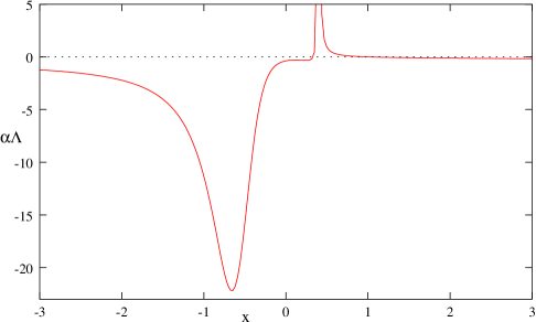
Figure 1: Variation of $\alpha\Lambda$ with respect to $x$, for $\zeta=4/3$ and $c_{2}=16/27$.

If we take the limit of $\alpha\to 0$, with $z_{*}$ and $\phi_{0}$ remaining finite, the $x<-1/2$ branch of solutions to (21) will disappear. We will be left with only $x>1$ solutions, which have singularities or infinite $M_{\mathrm{Pl}}$.

Alternatively we can rescale the dimensionful integration constant $z_{*}$, defining $\bar{z}_{*}=z_{*}/\sqrt{\alpha}$. Then going back to (20) we see that the $\alpha=0$ limit is badly behaved (Direct integration of the field equations gives an imaginary string coupling). This is not surprising since as eq. (17) already tells us, $\alpha=0$ and $\mathcal{C}=0$ are incompatible.

4 “Self-Tuning” Mechanism on the Brane

We now move on to the junction conditions which will relate our bulk parameters to the physical brane tension. We assume $Z_{2}$ reflection symmetry about $z=0$. The junction conditions at $z=0$ obtained from (14) and (16) are [22]

$$\left[3A^{\prime}+4\alpha e^{-\zeta\phi}(3\zeta\phi^{\prime}A^{\prime 2}-A^{\prime 3})\right]_{-}^{+}=-\lambda\ ,$$ (25)

$$\left[\zeta\phi^{\prime}-2\alpha e^{-\zeta\phi}(c_{2}\phi^{\prime 3}+8\zeta A^{\prime 3})\right]_{-}^{+}=\frac{d\lambda}{d\phi}\ .$$ (26)

Substituting in our solution we find that $\chi=\zeta/2$. Thus, for $\zeta=4/3$, $\chi=2/3$ which is is the value we would expect from a Neveu-Schwarz brane. This is thus absolutely consistent with our original choice of a heterotic string model.

We find that the brane tension $T$ satisfies

$$T=M_{s}^{3}\ e^{-\zeta\phi_{0}/2}\frac{(-8x)(6c_{2}-6\zeta^{4}x^{3}-\zeta^{3}x^{2}-6\zeta^{3}x)}{z_{*}(8c_{2}-9\zeta^{4}x^{3}-6\zeta^{4}x^{2})}\ .$$ (27)

However, as noticed earlier, $z_{*}$ is not an integration constant it is determined in terms of the parameters of the theory through (22). Thus we have

$$T=\frac{M_{s}^{3}}{\sqrt{\alpha}}\ (-4x)\ \frac{(6c_{2}-6\zeta^{4}x^{3}-\zeta^{3}x^{2}-6\zeta^{3}x)(4-3\zeta x)^{1/2}\zeta^{3/2}}{(8c_{2}-9\zeta^{4}x^{3}-6\zeta^{4}x^{2})^{3/2}}\ ,$$ (28)

which amounts to a fine-tuned relation among the parameters of the theory since $x$ is related to $\alpha\Lambda$ through (21).

We will now take again $\zeta=4/3$ and $c_{2}=16/27$ as a specific example. If $z_{*}>0$ and $x<0$ the tension is always positive, so our model uses a physical brane. When $z_{*}<0$ it has negative tension unless $x>0$ [22]. We note that, on the contrary, in the standard self-tuning solution, we have an opposite sign for $T$ and $z_{*}$ (see previous footnote).

Using equations (22),(24) and (28) we can obtain the string coupling and $M_{s}$ in terms of $M_{\mathrm{Pl}}$ and $T$. If $(-x)\gtrsim 1$, which is the case when $\alpha\Lambda$ is of order $-1$, we obtain the order of magnitude estimates

$$e^{\phi_{0}}\sim\frac{M_{s}^{3}}{M_{\mathrm{Pl}}^{3}}\ ,$$ (29)

$$T\sim M_{s}^{4}\ .$$ (30)

If we take $T\sim(1\mathrm{TeV})^{4}\sim 10^{-60}M_{Pl}^{4}$, we obtain $e^{\phi_{0}}\sim 10^{-45}$ which is obviously a ridiculously small value for the string coupling: we recover the typical fine-tuning associated with the cosmological constant. Of course, in the context of the weakly heterotic model, we expect $M_{s}$ to be much closer to the Planck scale. On the other hand, we see from eq. (24) that if $x$ is near to $-1/2$, we can obtain $e^{\phi_{0}}\sim 1$ when $M_{s}\ll M_{\mathrm{Pl}}$. However this requires severe fine-tuning of $x$.

5 Conclusions and outlook

In this paper we have shown the existence of a “quantum corrected” solution to the system with a bulk dilaton conformally coupled to matter on the brane, much as in the self-tuning set up. Unlike previous work on the subject our solution is free of naked singularities. It is expected to localize 4-dimensional gravity on the brane since the corresponding Planck scale is computed to be finite. The absence of a naked singularity allows us to study the issue of fine-tuning without ambiguity. We find that a fine tuning is necessary between the brane tension and the bulk vacuum energy (through our equations (28) and (21)).

It must be said however that the higher order corrections that we include do not resolve the singularity problems of the “self-tuning” solutions found in the $O(\alpha^{\prime 0})$ theory. Instead the $O(\alpha^{\prime})$ terms produce a completely new branch of well behaved solutions. Thus our approach differs from other approaches on the subject in that the solution no longer exists if the “quantum correction” is set to zero (see also [21, 22]). This is a genuine 5 dimensional $O(\alpha^{\prime})$ classical solution.

In the context of string theory and since we are relying on an effective action approach, the solution is well defined if higher order quantum gravity corrections in $\alpha^{\prime 2}$ [14] or quantum loop corrections in $g_{s}=e^{\phi}$ are not dominant. As we showed the string coupling is generically small in our model becoming of order 1 when $M_{s}\sim M_{pl}$. Furthermore it is easy to see that quantum gravity corrections in powers of $|\alpha^{\prime}R|$ become important as we get closer to the brane. This is not surprising, since according to Mach’s principle, spacetime is strongly curved where matter is localised. Since we are crudely modeling our universe by a Dirac distribution of tension $T$ our approximation will inevitably fail close to the brane. At this scale the fine structure of Standard Model physics becomes important. On the geometry or gravity side this is consistent with the fact that any higher order quantum gravity corrections in $\alpha^{\prime 2}$ would destroy the nice properties of Gauss-Bonnet gravity (see for example [20] and references within). Indeed, field equations would depend on higher derivatives in the metric, and distributional boundary conditions would be ill-defined! One would inevitably have to consider our brane as having some non-trivial $\alpha$-dependent thickness.

Any toy model, such as the one described here, suffers from its own limitations as an effective theory. For the ansatz we consider, one can argue that higher order curvature corrections in $\alpha^{\prime 2}$ [14] will increase the order of the algebraic equations for $x$. This could give rise to yet more solutions, although it is also possible that our solutions may disappear. A full solution to the cosmological constant problem has to rely on a quantum theory of gravity.

What we feel is important is the realisation that quantum corrections to ordinary Einstein gravity can be crucial in higher dimensional models. Even if one considers them at first order, as we do here, they are compatible with the principles of relativity theory for $D>4$. Indeed the Gauss-Bonnet action has to be included in the Einstein-Hilbert plus cosmological constant action in order for the gravity theory to be unique [16] in 5 dimensions. On the other hand these terms provide a window to the leading $\alpha^{\prime}$ gravity string corrections. Furthermore if there is to be a low string scale (of order 1 TeV) then these $\alpha^{\prime}$ corrections become more and more important.

An interesting direction of study is whether solutions of the type discussed in this paper exist if we allow a small cosmological constant on the brane, i.e. if the brane is $dS_{4}$ or $AdS_{4}$. Furthermore, the issue of stability is very important here. It is essential that the solution we propose is classicaly stable under small perturbations. Such a solution has to be a stable attractor for other solutions of the system if we really are to talk of a higher dimensional resolution of the cosmological constant problem. Furthermore localisation of 4-dimensional gravity is required in order to view this model as a new approach to a string theory realisation of the Randall-Sundrum model [9].

6 Acknowledgements

It is a great pleasure to thank Emilian Dudas, Christophe Grojean, Jihad Mourad, and Dani Steer for numerous discussions on the subject. We are indebted to Jihad Mourad for useful remarks.

References

- [1] A. Lukas, B. A. Ovrut, K. S. Stelle and D. Waldram, Phys. Rev. D 59 086001 (1999) [hep-th/9803235].
- [2] A. Lukas, B. A. Ovrut and D. Waldram, Phys. Rev. D 60 086001 (1999) [hep-th/9806022].
- [3] N. Arkani-Hamed, S. Dimopoulos and G. R. Dvali, Phys. Lett. B429 263 (1998) [hep-ph/9803315]; I. Antoniadis, N. Arkani-Hamed, S. Dimopoulos and G. R. Dvali, Phys. Lett. B436 257 (1998) [hep-ph/9804398].
- [4] P. Binétruy, C. Deffayet and D. Langlois, Nucl. Phys. B565 269 (2000) [hep-th/9905012].
- [5] L. Randall and R. Sundrum, Phys. Rev. Lett. 83 3370 (1999) [hep-ph/9905221].
- [6] V. A. Rubakov and M. E. Shaposhnikov, Phys. Lett. B125 136 (1983); K. Akama, in Gauge Theory and Gravitation. Proceedings of the International Symposium, Nara, Japan, 1982, eds. K. Kikkawa, N. Nakanishi and H. Nariai (Springer–Verlag, 1983).
- [7] V. A. Rubakov and M. E. Shaposhnikov, Phys. Lett. B125 139 (1983).
- [8] M. Visser, Phys. Lett. B159 22 (1985) [hep-th/9910093]; E. J. Squires, Phys. Lett. B167 286 (1986).
- [9] L. Randall and R. Sundrum, Phys. Rev. Lett. 83 4690 (1999) [hep-th/9906064].
- [10] N. Arkani-Hamed, S. Dimopoulos, N. Kaloper and R. Sundrum, Phys. Lett. B480 193 (2000) [hep-th/0001197]; S. Kachru, M. Schulz and E. Silverstein, Phys. Rev. D 62 045021 (2000) [hep-th/0001206].
- [11] C. Csaki, J. Erlich, C. Grojean and T. J. Hollowood, Nucl. Phys. B584 359 (2000) [hep-th/0004133].
- [12] C. Charmousis, Class. Quant. Grav. 19 83 (2002) [hep-th/0107126]; S. C. Davis, JHEP 0203 058 (2002) [hep-ph/0111351].
- [13] S. Förste, Z. Lalak, S. Lavignac and H. P. Nilles, Phys. Lett. B481 360 (2000) [hep-th/0002164]; S. P. de Alwis, Nucl. Phys. B597 263 (2001) [hep-th/0002174].
- [14] D. J. Gross and J. H. Sloan, Nucl. Phys. B291 41 (1987).
- [15] R. R. Metsaev and A. A. Tseytlin, Nucl. Phys. B293 385 (1987).
- [16] D. Lovelock, J. Math. Phys. 12 498 (1971).
- [17] B. Zwiebach, Phys. Lett. B156 315 (1985).
- [18] D. G. Boulware and S. Deser, Phys. Rev. Lett. 55 2656 (1985); J. Madore, Phys. Lett. A110 289 (1985); Phys. Lett. A111 283 (1985); J. T. Wheeler, Nucl. Phys. B268 737 (1986); N. Deruelle and J. Madore, Phys. Lett. A114 185 (1986), Phys. Lett. B186 25 (1987).
- [19] J. E. Kim, B. Kyae and H. M. Lee, Nucl. Phys. B582 296 (2000), Erratum: ibid. B591 587 (2000) [hep-th/0004005]; N. Deruelle and T. Dolezel, Phys. Rev. D 62 103502 (2000) [gr-qc/0004021]; J. E. Kim and H. M. Lee, Nucl. Phys. B602 346 (2001), Erratum: ibid. B619 763 (2001) [hep-th/0010093]; I. P. Neupane Phys. Lett. B512 (2001) 137 [hep-th/0104226]; K. A. Meissner and M. Olechowski, Phys. Rev. D 65 064017 (2002) [hep-th/0106203]. B. Abdesselam and N. Mohammedi, Phys. Rev. D 65 084018 (2002) [hep-th/0110143]; C. Germani and C. F. Sopuerta, hep-th/0202060.
- [20] C. Charmousis and J. F. Dufaux, hep-th/0202107.
- [21] N. E. Mavromatos and J. Rizos, Phys. Rev. D 62 124004 (2000) [hep-th/0008074].
- [22] N. E. Mavromatos and J. Rizos, hep-th/0205299.
- [23] I. Low and A. Zee, Nucl. Phys. B585 395 (2000) [hep-th/0004124].
- [24] E. S. Fradkin and A. A. Tseytlin, Phys. Lett. B158 316 (1985); Nucl. Phys. B261 1 (1985).
- [25] R. C. Myers, Phys. Lett. B199, 371 (1987).
- [26] S. Weinberg, Rev. Mod. Phys. 61 1 (1989).
- [27] S. Dasgupta, R. Venkatachalapathy, S. Kalyana Rama, hep-th/0204136.
- [28] J. M. Cline and H. Firouzjahi, Phys. Rev. D 65 043501 (2002) [hep-th/0107198].
- [29] I. Antoniadis, J. Rizos and K. Tamvakis, Nucl. Phys. B415 497 (1994) [hep-th/9305025].