Inflationary Theory and Alternative Cosmology

Abstract:

Recently Hollands and Wald argued that inflation does not solve any of the major cosmological problems. We explain why we disagree with their arguments. They also proposed a new speculative mechanism of generation of density perturbations. We show that in their scenario the inhomogeneities responsible for the large scale structure observed today were generated at an epoch when the energy density of the hot universe was $10^{95}$ times greater than the Planck density. The only way to avoid this problem is to assume that there was a stage of inflation in the early universe.

1 Introduction

During the last 20 years inflationary theory [1, 2, 3] has evolved from a problematic hypothesis to an almost universally accepted cosmological paradigm [4]. It solves many fundamental cosmological problems and makes several predictions that agree very well with the observational data [5]. Despite this fact (or maybe because of it) it has become popular to propose various alternatives to inflation.

In this paper we will consider one such alternative suggested recently by Hollands and Wald [6]. The authors admit that their model does not solve or even address the homogeneity, isotropy, flatness, horizon and entropy problems, but they claim that inflation does not do so either. We will examine their claim and explain why we disagree with it. We will use this discussion as an opportunity to emphasize some properties of inflation that may not be widely known.

What Hollands and Wald’s model does attempt to explain is the generation of density perturbations with a flat spectrum. However, one cannot justify this mechanism using the standard methods of quantum field theory. Moreover, in this scenario density perturbations on the scale of the present horizon were generated at a time when the energy density of the hot universe was $10^{95}$ times greater than the Planck density. Since nobody knows how to make any calculations at such densities, one must be hard pressed to consider this an alternative to the inflationary mechanism of generation of density perturbations. We will explain that the origin of this problem is directly related to the absence of inflation in the model proposed in [6].

2 Fluctuations in the model with fundamental scale without inflation

We will begin our discussion of the paper by Hollands and Wald [6] by describing their proposed mechanism for the generation of cosmological fluctuations without inflation.

Consider for definiteness radiation-dominated cosmological expansion that begins at a singularity at $t=0$, with a scale factor $a(t)=\sqrt{t}$. According to [6], one should introduce a new “fundamental scale” $l_{0}\sim 10^{-5}M_{p}^{-1}\sim 10^{-28}$ cm. It is assumed in [6] that quantum fluctuations evolve according to QFT only in the regime where their physical wavelengths exceed the fundamental length, $\lambda(t)\geq l_{0}$, where initially $l_{0}$ is much greater than the Hubble radius $H^{-1}$.

In inflationary theory quantum fluctuations oscillate until their wavelength reaches $H^{-1}$. After that they freeze with amplitude $\delta\phi\sim{H\over 2\pi}$. This amplitude can be calculated using standard quantum field theory methods [7] and then it can be used to calculate the amplitude of inflationary density perturbations [8].

But fluctuations with wavelength greater than $H^{-1}$ do not oscillate even if the universe is not inflationary. As a result, from the very beginning of their QFT phase, quantum fluctuations in the scenario proposed in [6] are frozen with almost constant amplitude, which is supposed to be $\delta\phi\sim{l_{0}}^{-1}$. This last assumption does not follow from quantum field theory in curved space. This could be a reasonable assumption if $l_{0}^{-1}$ were the largest parameter of dimension of mass, but the authors use this assumption in the situation when $H\gg l_{0}^{-1}$, i.e. when the size of the horizon $H^{-1}$ is much smaller than the fundamental length $l_{0}$. We will return to this important point later. However, if this assumption is correct, the spectrum of perturbations generated by this mechanism for $l_{0}\sim 10^{-5}M_{p}$ can be comparable to the spectrum of standard inflationary perturbations.

One can estimate the time $t_{*}$ when the fluctuations corresponding to the present cosmological horizon $10^{28}$ cm were frozen. If the scale factor at present is unity, then

$$a(t_{*})=\frac{l_{0}}{10^{28}cm}\simeq 10^{-56}\ .$$ (1)

The density of radiation today is $\rho_{r}\simeq 10^{-35}$g/cm${}^{3}\sim 10^{-129}M_{p}^{4}$. This density at the time $t_{*}$ was greater by a factor of $a^{-4}(t_{*})\sim 10^{224}$. Therefore at the moment $t_{*}$ the density of radiation was

$$\rho_{r}(t_{*})\simeq 10^{95}M_{p}^{4}\ .$$ (2)

Here $M_{p}^{4}\simeq 10^{94}$ g/cm³ is the Planck density, $M_{p}=G^{-1/2}\sim 10^{19}$ GeV.

But this means that all assumptions concerning the generation of perturbations made in [6] are completely unreliable. Indeed, quantum fluctuations of the curvature of space and time at densities $95$ orders of magnitude greater than the Planck density are so large that any discussion of the universe in terms of classical space-time becomes impossible.

One can easily verify that this problem appears not only in a radiation dominated universe with $p=\rho/3$, but for all equations of state $p=\omega\rho$ with $0<\omega<1$ considered in [6]. Indeed, let us assume that physical laws up to the electroweak scale $T_{{}_{\rm EW}}\sim 10^{2}$ GeV are well known, so the universe was radiation dominated when it had electroweak scale energy density. We will also assume that before the electroweak stage the equation of state was $p=\omega\rho$.

At the electroweak stage the scale factor $a_{{}_{\rm EW}}$ was smaller than at the present time by a factor of $2.7K^{o}/T_{{}_{\rm EW}}\sim 10^{-15}$, and the density was $\rho_{{}_{\rm EW}}=O(T^{4}_{{}_{\rm EW}})\sim 10^{-68}M_{p}^{4}$. The density perturbations on the scale of the present horizon were generated at an epoch when the scale factor was $a(t_{*})=10^{-56}=10^{41}a_{{}_{\rm EW}}$, and the density was

$$\rho_{r}(t_{*})\simeq\rho_{{}_{\rm EW}}\left({a_{{}_{\rm EW}}\over a(t_{*})}\right)^{3(1+\omega)}=10^{-68}M_{p}^{4}\times 10^{41(3(1+\omega))}\ .$$ (3)

This corresponds to a density smaller than $M_{P}^{4}$ only if $\omega<-{55\over 123}\sim-0.45$. This means that $p<-0.45\rho$ and $\rho+3p<-0.3\rho$, which corresponds to an accelerating (=inflating) universe with negative pressure. If the standard regime $p=\omega\rho$ with $0<\omega<1$ took place all the way up to the GUT scale, one can show that $\rho_{r}(t_{*})<M_{p}^{4}$ only if $p\approx-\rho$ above the GUT scale. In other words, in order to avoid speculations about super-Planckian densities in the mechanism of generation of density perturbations proposed in [6] one must have a stage of inflation in the early universe. Thus, the mechanism of [6] does not offer any alternative to inflation because it needs inflation for its own consistency.

The main difference between the models with “normal” equations of state $0<\omega<1$ considered in [6] and inflationary cosmology is the following. In the simplest versions of inflationary cosmology the fluctuations responsible for the observed CMB anisotropy also freeze on a length scale $\sim 10^{-5}M_{p}^{-1}$, and then their wavelengths grow until they reach $10^{28}$ cm. However, the energy density of the universe does not change much during the first 60 e-folds of this growth. That is why if one takes perturbations on the scale $10^{28}$ cm and follows their evolution back in time, one finds that they were produced during the stage of inflation when the energy density was many orders of magnitude smaller  than the Planck density. This is one of the many amazing features of inflationary cosmology. The attempt to reproduce inflationary results [6] fails exactly because the authors were trying to achieve them without using an early stage of inflation. Paradoxically, evaluation of the “alternative to inflation” proposed in [6] provides an additional argument in favour of inflation.

In fact, the situation with the mechanism proposed in [6] is even more problematic. Consider again a radiation dominated universe at the time $t_{*}$. The Hubble constant at that time is $10^{52}$ times greater than $l_{0}^{-1}$ and the temperature is $10^{29}$ times greater than $l_{0}^{-1}$. But how could it be possible that the wavelength of the high-energy particles $T^{-1}$ is $29$ orders of magnitude smaller than the “elementary length” $l_{0}$, and the size of horizon is $52$ orders of magnitude smaller than the “elementary length” $l_{0}$? This contradicts the basic assumptions of [6]. And even if this were possible, then the standard quantum field theory considerations would suggest that at the time $t_{*}$ the amplitude of fluctuations would be determined not by $l_{0}$, but by the greatest of these dimensional parameters, i.e. it would be expected to be $10^{52}$ times greater than the amplitude postulated in [6].

Note that this problem persists even if one would attempt to apply the prescription by Hollands and Wald to the generation of density perturbations during inflation, where the energy density remains below the Planck density. Indeed, the basic idea of this prescription is that the wavelength and the amplitude of perturbations generated at $H\gg l_{0}$ should be determined only by $l_{0}$. According to inflationary theory, the amplitude of quantum fluctuations generated during inflation is determined by the Hawking temperature in de Sitter space, $\delta\phi\sim T_{H}={H\over 2\pi}$. We have no idea how one could justify an assumption of [6] that the amplitude of perturbations produced during inflation should be $\sim l_{0}^{-1}$, which is much smaller than the Hawking temperature during inflation. We believe that it is inconsistent to assume that the size of the horizon in de Sitter space $H^{-1}$ is much smaller than the “elementary length” $l_{0}$.

3 Initial conditions for inflation

A significant part of [6] was devoted to a discussion of the problem of initial conditions for inflation. In this section we will describe the simplest model of chaotic inflation and consider the issue of initial conditions. Then we will compare our analysis and the arguments of [6].

3.1 Initial conditions for chaotic inflation

Consider the simplest model of a scalar field $\phi$ with a mass $m$ and with the potential energy density $V(\phi)={m^{2}\over 2}\phi^{2}$. (One may also add a cosmological constant $V_{0}\sim 10^{-123}M_{p}^{4}$ to describe the present stage of acceleration of the universe.) Since this function has a minimum at $\phi=0$, one may expect that the scalar field $\phi$ should oscillate near this minimum. This is indeed the case if the universe does not expand, in which case the equation of motion for the scalar field coincides with the equation for a harmonic oscillator, $\ddot{\phi}=-m^{2}\phi$.

However, because of the expansion of the universe with Hubble constant $H=\dot{a}/a$, an additional term $3H\dot{\phi}$ appears in the harmonic oscillator equation:

$$\ddot{\phi}+3H\dot{\phi}=-m^{2}\phi\ .$$ (4)

The term $3H\dot{\phi}$ can be interpreted as a friction term. The Einstein equation for a homogeneous universe dominated by a scalar field $\phi$ looks as follows:

$$H^{2}+{k\over a^{2}}={8\pi\over 6}\,\left(\dot{\phi}^{2}+m^{2}\phi^{2}\right)\ .$$ (5)

Here $k=-1,0,1$ for an open, flat or closed universe respectively. For simplicity, we work in units $M_{p}^{-2}=G=1$.

If the scalar field $\phi$ initially was large, the Hubble parameter $H$ was large too, according to the second equation. This means that the friction term $3H\dot{\phi}$ was very large, and therefore the scalar field was moving very slowly. At this stage the energy density of the scalar field remained almost constant, and the expansion of the universe continued with a much greater speed than in the old cosmological theory. Due to the rapid growth of the scale of the universe and a slow motion of the field $\phi$, soon after the beginning of this regime one has $\ddot{\phi}\ll 3H\dot{\phi}$, $H^{2}\gg{k\over a^{2}}$, $\dot{\phi}^{2}\ll m^{2}\phi^{2}$, so the system of equations can be simplified:

$$H={\dot{a}\over a}=2m|\phi|\sqrt{\pi\over 3}\ ,~{}~{}~{}~{}~{}~{}\dot{\phi}=\pm{m\over 2\sqrt{3\pi}}.$$ (6)

The first equation shows that if the field $\phi$ changes slowly, the size of the universe in this regime grows approximately as $e^{Ht}$, where $H=2m|\phi|\sqrt{\pi\over 3}$. This is the stage of inflation, which ends when the field $\phi$ becomes much smaller than $M_{p}=1$. A universe initially filled with a field $\phi=\phi_{0}\gg 1$ will experience a long stage of inflation and grow exponentially large.

The issue of initial conditions in this scenario has been analysed using various methods including Euclidean quantum gravity, the stochastic approach to inflation, etc., see e.g. [4]. Here we would like to take a simple intuitive approach.

Consider, for definiteness, a closed universe of initial size $l\sim 1$ (in Planck units) that emerges from the space-time foam, or from a singularity, or from ‘nothing,’ in a state with Planck density $\rho\sim 1$. Only starting from this moment, i.e. at $\rho\mathrel{\hbox{\hbox to0.0pt{\hbox{\lower 4.0pt\hbox{$\sim$}}\hss}\hbox{$<$}}}1$, can we describe this domain as a classical universe. Thus, at this initial moment the sum of the kinetic energy density, gradient energy density, and potential energy density is of order unity:  ${1\over 2}\dot{\phi}^{2}+{1\over 2}(\partial_{i}\phi)^{2}+V(\phi)\sim 1$.

It is important to understand that in this model there are no a priori constraints on the initial value of the scalar field in this domain, except for the constraint ${1\over 2}\dot{\phi}^{2}+{1\over 2}(\partial_{i}\phi)^{2}+V(\phi)\sim 1$. Indeed, let us consider for a moment a theory with $V(\phi)=const$. This theory is invariant under the shift $\phi\to\phi+c$. Therefore, in such a theory all initial values of the homogeneous component of the scalar field $\phi$ are equally probable. Contrary to some assertions in the literature, quantum gravity corrections do not lead to any constraints of the type $\phi<1$ [4]. Such corrections may affect the potential if, e.g., one tries to incorporate this model into N=1 supergravity. But this is a separate issue of model building rather than the issue of initial conditions for our simple model. The only constraint on the average amplitude of the field appears if the effective potential is not constant, but grows and becomes greater than the Planck density at $\phi>\phi_{p}$, where $V(\phi_{p})=1$. This constraint implies that $\phi\mathrel{\hbox{\hbox to0.0pt{\hbox{\lower 4.0pt\hbox{$\sim$}}\hss}\hbox{$<$}}}\phi_{p}$, but it does not give any reason to expect that $\phi\ll\phi_{p}$. This suggests that the typical initial value $\phi_{0}$ of the field $\phi$ in such a theory is $\phi_{0}\sim\phi_{p}$. Thus, we expect that typical initial conditions correspond to ${1\over 2}\dot{\phi}^{2}\sim{1\over 2}(\partial_{i}\phi)^{2}\sim V(\phi)=O(1)$. If by any chance ${1\over 2}\dot{\phi}^{2}+{1\over 2}(\partial_{i}\phi)^{2}\mathrel{\hbox{\hbox to0.0pt{\hbox{\lower 4.0pt\hbox{$\sim$}}\hss}\hbox{$<$}}}V(\phi)$ in the domain under consideration, then inflation begins, and within a Planck time the terms ${1\over 2}\dot{\phi}^{2}$ and ${1\over 2}(\partial_{i}\phi)^{2}$ become much smaller than $V(\phi)$, which ensures the continuation of inflation. The probability of such an event may be equal to $1/2$, or $10^{-1}$, or maybe even $10^{-2}$, but there’s no obvious reason why it should be exponentially suppressed. Moreover, the total lifetime of a non-inflationary universe with ${1\over 2}\dot{\phi}^{2}+{1\over 2}(\partial_{i}\phi)^{2}>V(\phi)$ is $O(1)$ in Planck units, i.e. $10^{-43}$ seconds. Such universes are unsuitable for the existence of any observers. The lifetime $10^{-43}$ seconds is shorter than the lifetime of any virtual particle, so one may argue that non-inflationary universes with ${1\over 2}\dot{\phi}^{2}+{1\over 2}(\partial_{i}\phi)^{2}>V(\phi)$ do not really exist at the classical level. Meanwhile all universes with ${1\over 2}\dot{\phi}^{2}+{1\over 2}(\partial_{i}\phi)^{2}\mathrel{\hbox{\hbox to0.0pt{\hbox{\lower 4.0pt\hbox{$\sim$}}\hss}\hbox{$<$}}}V(\phi)$ exist for an exponentially long time and become exponentially large. It seems therefore that chaotic inflation occurs under rather natural initial conditions, if it can begin at $V(\phi)\sim 1$ [3, 4]. If one discards universes with a total lifetime smaller than $10^{-40}$ seconds, just as one discards subcritical bubbles during tunneling, then one may argue that most of the universes with a macroscopically large lifetime are inflationary.

Similar conclusions can be obtained if one considers the probability of quantum creation of the universe from nothing. According to [9], the probability of quantum creation of the universe is suppressed by $e^{-S}$, where $S={3\over 8V(\phi)}$ is the entropy of de Sitter space. This implies that creation of a closed universe is most probable at $V(\phi)\sim 1$, and it is exponentially suppressed for $V(\phi)\ll 1$. For example, the typical energy density during inflation in new inflation scenario is $V(\phi)\sim M^{4}_{\rm GUT}\sim 10^{-12}$; quantum creation of the universe in such theories is suppressed by $e^{-10^{12}}$. Meanwhile in the simplest versions of chaotic inflation with $V(\phi)\sim\phi^{n}$ inflation is possible for $V(\phi)$ close to the Planck density as well as below it, and the creation of inflationary universes is not exponentially suppressed. A similar result can be obtained by a combinatorial analysis proposed in [10].

A simple way to understand this argument is to consider the usual uncertainty relation $\Delta E\Delta t\sim 1$. The total energy of matter in a closed inflationary universe is proportional to the volume of the “throat” of de Sitter hyperboloid $H^{-3}\sim M_{p}^{3}V^{-3/2}$ multiplied by the energy density $V$. This gives $\Delta E\sim M_{p}^{3}V^{-1/2}$. For $V\sim M_{p}^{4}$ one finds $\Delta E\sim M_{p}$, so there is no problem, according to the uncertainty relation $\Delta E\Delta t\sim 1$, with creating a Planck size closed inflationary universe with $V\sim M_{p}^{4}$ during the Planck time $\Delta t\sim M_{p}^{-1}$.

We are going to return to this issue in a separate publication. The main reason why we discussed it here was to present a general description of initial conditions for chaotic inflation. As we see, inflation may easily occur in a domain of a smallest possible size $O(M_{p}^{-1})=O(1)$. The universe initially may have a total mass as small as $M_{p}=1\sim 10^{-5}$ g and it may contain no elementary particles at all. The expansion of this domain gives rise to a domain of size $l\sim\exp{2\pi\phi_{p}^{2}}\sim\exp{2\pi m^{-2}}\sim 10^{10^{12}}$ [3, 4]. The decay of the scalar field at the end of inflation [11, 12] creates about $10^{10^{12}}$ elementary particles; we see only a minor part of them ($\sim 10^{88}$ particles) in the observable part of the universe.

Moreover, once inflation begins in an interval $m^{-1/2}<\phi_{0}<m^{-1}$ in the theory $m^{2}\phi^{2}/2$, the universe enters an eternal process of self-reproduction [13, 14]. Thus, if inflation begins in a single domain of the smallest possible size $l=O(1)$, it makes the universe locally homogeneous and produces infinitely many inflationary domains of exponentially large size. This makes the whole issue of initial conditions nearly irrelevant: Non-inflationary domains die within Planckian time, i.e. effectively remain unborn, whereas inflationary domains exist for a long time and produce infinitely many other inflationary domains.

3.2 Comparison with the argument by Hollands and Wald

Now we should try to compare this picture with the argument by Hollands and Wald suggesting that the initial conditions for inflation cannot be natural. They formulated their argument in the following form:

Let $\mathcal{U}$ be the collection of universes that start from a “big bang” type of singularity, expand to a large size and recollapse to a “big crunch” type of singularity. Let $\mathcal{I}$ denote the space of initial data for such universes and let $\mu_{\mathcal{I}}$ denote the measure on this space used by the “blindfolded Creator”. Let $\mathcal{F}$ denote the space of final data of the universes in $\mathcal{U}$, and let $\mu_{\mathcal{F}}$ denote the measure on $\mathcal{F}$ obtained from $\mu_{\mathcal{I}}$ via the “time reversal” map. Suppose that $\mu_{\mathcal{I}}$ is such that dynamical evolution from $\mathcal{I}$ to $\mathcal{F}$ is measure preserving (“Liouville’s theorem”). Then the probability that a universe in $\mathcal{U}$ gets large by undergoing an era of inflation is equal to the probability that a universe in $\mathcal{U}$ will undergo an era of “deflation” when it recollapses. Then the authors noted that the probability that a universe dominated by ordinary matter will deflate is very small. From their perspective, this implies, by time reversal invariance, that the probability of inflation must also be very small.

As we see, this argument is completely unrelated to the investigation of initial conditions for chaotic inflation performed in the previous section. It is based on several formal assumptions about the evolution of the universe that Hollands and Wald consider natural. First of all, they consider a recollapsing universe. Such a recollapse will not occur in our universe if we have a small cosmological constant leading to the present stage of acceleration. However, this is a minor problem since one can consider a formal time reversal at any moment of time.

The most important assumption is that dynamical evolution is measure preserving, which, roughly speaking, means that the number of degrees of freedom does not change during inflationary evolution. This assumption often holds for dynamical systems ignoring particle production. However, in application to inflationary cosmology this assumption is definitely incorrect. Indeed, in inflationary cosmology the total energy and entropy of the scalar field and particles created by its decay is not conserved. In our simple scenario the total initial mass of matter in the universe was $O(1)\sim 10^{-5}$ g, but later on its total energy became exponentially large. In terms of particle physics, measure preservation implies conservation of the number of particles. But in chaotic inflation initially we did not have any particles at all, the total entropy was $O(1)$, and then we got more than $10^{10^{12}}$ particles with entropy greater than $10^{10^{12}}$. The absence of adiabaticity is a key feature of all inflationary models because inflation removes all particles that could be present before inflation; all $10^{88}$ particles that we see now within our cosmological horizon were created by the decaying scalar field.

Decay of the scalar field and particle production are irreversible processes, and therefore, quite independently of the issue of probabilities, time reversal of inflationary evolution can never produce the same initial conditions the universe started with. The scalar field that decayed at the end of inflation is not going to re-appear again if one reverses the time evolution. The number of particles produced by this field, just as the inhomogeneities produced during inflation, will only grow on the way back to the singularity.

Initially our universe could have had Planck size and Planck mass at the moment when it had Planck density. But then it became exponentially large and heavy. Time-reversal of its evolution would lead to an exponentially large and exponentially heavy universe at the moment when it reached Planck density on its way back to the singularity. Indeed, at the Planck density each Planck size volume can contain no more than one particle with Planckian temperature. This means that if the observable part of the universe (which is many orders of magnitude smaller than the whole inflationary universe at present) were to recollapse, it would consist of more than $10^{88}$ Planck size domains at the Planck density. And the whole universe containing $10^{10^{12}}$ particles (even if we ignore self-reproduction that makes this number indefinitely large) would consist of $10^{10^{12}}$ Planck size domains at the Planck density. We cannot squeeze the universe back to its initial Planckian size by time reversal.

Similarly, large scale cosmological inhomogeneities created by quantum fluctuations are not going to disappear under time reversal. Even if the inflationary universe was ideally homogeneous from the very beginning, time reversal of its evolution from the present stage would never return it to its original form.

Thus, inflationary evolution is irreversible, and the ‘obvious’ requirement of measure preserving evolution is not satisfied in inflationary cosmology. Information contained in the single Planck size initial inflationary domain is insufficient to predict the speed and position of each of the $10^{10^{12}}$ particles created after inflation. And even if we were able to know exactly the final conditions after inflation including the speed and position of each of the $10^{10^{12}}$ particles created after inflation, this would not help us to squeeze all of these particles into the initial domain of the Planck size. This irreversibility comes about because the elementary particles and even galaxies that we see now appeared as a result of random quantum processes that could not be predicted by imposing initial conditions on the evolution of the classical scalar field $\phi$ in the initial Planck size domain. This invalidates the argument of Hollands and Wald against inflation.

These issues are deeply related to the discussion of reversibility in quantum cosmology contained in the famous paper by Bryce DeWitt [17] (see also the well-known paper by Hawking [18] and comments by Don Page [19]). All equations of general relativity are time reversal invariant, and therefore there are an equal number of universes with growing and decreasing entropy. However, once we pick up a large classical universe and define time there, the entropy and the total number of particles inside this universe can only grow. Similarly, once we consider a particular realization of an inflationary universe after it becomes large and the scalar field decays producing many particles, these particles cannot be un-born on the way back to the singularity.

But even if we ignore quantum effects and particle production, and even if it were possible to recreate the initial inflationary domain by time reversal, this would not mean that investigation of the final conditions after inflation can tell us anything about the probability of initial conditions for inflation. Indeed, the inflationary regime with $p\approx-\rho$ is an attractor in the phase space $(\phi,\dot{\phi})$ during expansion of the universe. Meanwhile during the stage of collapse, the deflationary trajectory with $p\approx-\rho$ is repulsive, and all trajectories are attracted to the regime with the stiff equation of state $p\approx+\rho$ [16]. Therefore the fact that the collapsing universe typically does not deflate is completely compatible with the possibility that the natural initial conditions in the early universe lead to inflation. We will consider a particular example illustrating this general statement in the next section.

3.3 Inflationary regime as an attractor

In this section we will discuss one of the aspects of the theory of initial conditions for inflation. For illustrative purposes, we will consider the simplest model $m^{2}\phi^{2}/2$ and study the evolution of the homogeneous field $\phi$ in a flat universe filled with radiation. Our goal here is not to study the most general initial conditions for inflation in a flat universe, but to illustrate on a simple example some basic issues related to the choice of initial conditions versus final conditions. For convenience, in this section we measure time in units of $m^{-1}$.

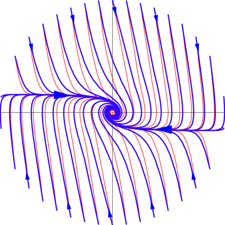
Figure 1: Phase portrait for the theory $V(\phi)={1\over 2}m^{2}\phi^{2}$. The blue (thick) lines show trajectories describing the universe without radiation. The scalar field has half Planck density at the beginning of the simulations. The red (thin) lines show trajectories where an equal amount of energy in radiation was added to the system. In both cases the velocity of the scalar field rapidly decreases, which usually leads to the onset of inflation. The inflationary separatrices (the horizontal lines to which most of the trajectories converge) are attractors when we move forwards in time, but they will be repulsors if we reverse direction of time and move from the center back to large $|\phi|$ and $|\dot{\phi}|$.

The phase portrait of this model in the space of the variables $(\phi,\dot{\phi})$ is shown in Fig 1 [16]. The red (thin) lines in this figure show the evolution of $(\phi,\dot{\phi})$ in a universe filled with radiation. Evolution begins at the Planck density sphere ${m^{2}\over 2}(\dot{\phi}^{2}+\phi^{2})+\rho_{\rm rad}=1$, where $\rho_{\rm rad}$ is the energy density of radiation. (Recall that we are using time in units of $m^{-1}$.) The plot describes the situation where initially the energy was equally distributed between the scalar field and radiation. For comparison we also show the trajectories of the scalar field in the absence of radiation (thick blue lines).

As we see, most of the trajectories starting at the Planck density approach the inflationary attractors $\dot{\phi}=\pm{1\over 2\sqrt{3\pi}}$. In the Figure we have shown the process for the unrealistically large mass $m=1$. The situation becomes much more impressive in the realistic case $m\sim 10^{-6}$. Indeed, one can show that the fraction of trajectories not approaching inflation is smaller than $O(m^{-1})$ [15, 16].

The simplest way to see this is to consider a regime where in the beginning of the process one has $\rho_{\rm rad}\sim{m^{2}\over 2}(\dot{\phi}^{2}+\phi^{2})$ for $\phi\gg 1$, see red (thin) lines in Fig. 1. The kinetic energy of the scalar field $\dot{\phi}^{2}/2$ in this regime decreases as $a^{-6}$. Meanwhile, the density of radiation decreases as $a^{-4}$. Therefore the energy density of radiation eventually becomes greater than $\dot{\phi}^{2}/2$. As we will see, once this occurs the field rapidly slows down or even completely freezes. This provides good initial conditions for a subsequent stage of inflation [15, 16].

Consider the moment $t_{0}$ when the energy density of radiation becomes greater than $\dot{\phi}^{2}/2$. In this regime (and neglecting $V(\phi)$) one can show that $\dot{\phi}=\dot{\phi}_{0}{a_{0}^{3}\over a^{3}}=\dot{\phi}_{0}\left({t_{0}\over t}\right)^{3/2}$. Even if this regime continues for an indefinitely long time, the total change of the field $\phi$ during this time remains quite limited. Indeed,

$$\Delta\phi\leq\int\limits_{t_{0}}^{\infty}\dot{\phi}dt=\dot{\phi}_{0}\int\limits_{t_{0}}^{\infty}\left({t_{0}\over t}\right)^{3\over 2}dt=2~{}\dot{\phi}_{0}t_{0}.$$ (7)

If $t_{0}$ is the very beginning of radiation domination, then one has $m^{2}\dot{\phi}_{0}^{2}/2\sim\rho_{\rm total}/2={3H_{0}^{2}\over 8\pi}$. This implies that $H_{0}\sim mt_{0}^{-1}\sim 3m\dot{\phi}_{0}$. Therefore

$$\Delta\phi<1$$ (8)

in Planck units (i.e. $\Delta\phi<M_{p}$).

This simple result has several important implications. In particular, if the motion of the field in a radiation-dominated universe begins at $|\phi|\gg 1$, then it can move only by $\Delta\phi\mathrel{\hbox{\hbox to0.0pt{\hbox{\lower 4.0pt\hbox{$\sim$}}\hss}\hbox{$<$}}}1$. Therefore in theories with flat potentials the field always remains frozen at $|\phi|\gg 1$. It begins moving again only when the Hubble constant decreases and $|3H\dot{\phi}|$ becomes comparable to $|V,_{\phi}|$. But in this case the condition $3H\dot{\phi}\approx|V,_{\phi}|$ automatically leads to inflation in such theories as $m^{2}\phi^{2}/2$ for $\phi\gg 1$. This means that all trajectories starting at $|\phi|>1$ enter a stage of inflation. Since the field $\phi$ initially can take any value in the interval from $-m^{-1}$ to $m^{-1}$, and inflation does not happen only for $|\phi|\mathrel{\hbox{\hbox to0.0pt{\hbox{\lower 4.0pt\hbox{$\sim$}}\hss}\hbox{$<$}}}1$, the fraction of non-inflationary trajectories is $O(m^{-1})$ [15, 16]. For $m=10^{-6}$ this means that out of a million trajectories equally distributed over the initial Planckian sphere ${m^{2}\over 2}(\dot{\phi}^{2}+\phi^{2})=1$ only one trajectory will be non-inflationary!

One can represent the position of the vector $(\phi,\dot{\phi})$ at the Planckian sphere ${m^{2}\over 2}(\dot{\phi}^{2}+\phi^{2})=1$ by introducing the angle $\theta_{i}$ such that initially $\phi={\sqrt{2}\over m}\cos\theta_{i}$, $\dot{\phi}={\sqrt{2}\over m}\sin\theta_{i}$. Then the assumption of equal distribution over the sphere ${m^{2}\over 2}(\dot{\phi}^{2}+\phi^{2})=1$ implies that all values of $\theta_{i}$ are equally probable. In this case, as we have seen, the probability to have inflation is $1-O(m)\approx 1$.

Let us see, however, what will happen if we impose a similar condition after the end of inflation. When the field $\phi$ becomes much smaller than $1$, inflation ends. At this stage $\phi$ begins oscillating near the minimum of the effective potential at $\phi=0$ and the vector $(\phi,\dot{\phi})$ begins rotating around the origin in the phase space (i.e. around the point $(\phi=0,\dot{\phi}=0)$) with a slowly decreasing amplitude. After a long time, the decrease of the amplitude during each oscillation becomes extremely small, so the phase portrait becomes similar to the phase portrait of a simple harmonic oscillator, $(\phi=\phi_{f}\cos(t+\theta_{f}),\dot{\phi}=\phi_{f}\sin(t+\theta_{f}))$), where $\theta_{f}$ depends on the initial values of $(\phi,\dot{\phi})$ at the Planck time, i.e. on $\theta_{i}$. According to our analysis, almost all trajectories in the interval $-\pi<\theta_{i}<\pi$ will approach the inflationary separatrix, Fig. 1, and therefore almost all trajectories after inflation will have the same value of $\theta_{f}$. There will be some trajectories with different values of $\theta_{f}$, but the “density” of such trajectories will be suppressed by the factor $O(m^{-1})\sim 10^{-6}$.

Now let us make a time-reversal and consider the state of this harmonic oscillator as an initial state for the trajectories going back to the singularity. The initial state for this process is described by $\phi_{f}$ and $\theta_{f}$. A priori, no initial phase $\theta_{f}$ is any better than any other phase. Therefore the natural probability measure for initial conditions in the time-reversed universe should not depend on $\theta_{f}$. But we know that only a fraction of $O(m^{-1})\sim 10^{-6}$ out of the total range of the values of $\theta_{f}$ in the interval from $0$ to $2\pi$ correspond to inflationary trajectories.

Thus, from the point of view of the natural measure on space of initial conditions (equal density of trajectories crossing the Planck sphere ${m^{2}\over 2}(\dot{\phi}^{2}+\phi^{2})+\rho_{\rm rad}=1$) the probability to have inflation is $1-O(m^{-1})=1-O(10^{-6})$. Meanwhile, if one studies the same process from the point of view of the time-reversal process and uses the natural probability measure on space of final conditions, as suggested by Hollands and Wald, one finds that the probability of inflation is $10^{-6}$. But this trick in fact says nothing about the probability of inflation; it just a reflection of the well-known fact that even though dynamical equations are time-symmetric, the initial and final conditions are not interchangeable. The fact that the inflationary separatrix is a repulsor and the probability of deflation is $10^{-6}$ when we move back in time does not have any implications for the probability of inflation when we move forward in time. Indeed, when we move forward in time, the inflationary separatrix is an attractor, see Fig. 1, and the probability of inflation in this model is $1-O(m^{-1})=1-O(10^{-6})$.

If one considers the possibility of an inhomogeneous distribution of the scalar field, the probability of inflation becomes somewhat smaller but still remains large in the model under consideration, just like in the closed universe case considered in Section 3.1, see [3, 4, 14].

Note, that in this section we considered the simplest, intuitive choice of measure on the space of initial conditions for $\phi$ and $\dot{\phi}$, following [15]. Holland and Wald assumed that there should exist a canonical measure preserved during the dynamical evolution in accordance with the Liouville’s theorem. Indeed, a canonical measure in space of all dynamical variables $a$, $\dot{a}$, $\phi$, $\dot{\phi}$ does exist [20, 21, 22]. One could expect that by using this measure one can evaluate the probability of inflation in the early universe by considering various conditions at the late stages of the evolution of the universe and then going back in time, as suggested by Hollands and Wald.

However, it turns out that the use of the canonical measure [20, 21, 22] does not imply that the results of calculation of the probability of inflation are invariant along the trajectories. The integrals involving this measure diverge, which makes the results ambiguous and depending on the cosmic time when the probability is evaluated [22]. According to [22], if one investigates the probability of inflation using this measure starting at very low energy density, the probability of inflation could seem very small. However, if one imposes initial conditions at large energy density (i.e. in the very early universe), the probability of inflation appears very large. In particular, if one imposes initial conditions at the Planck time, which is the most reasonable choice because only after that moment one can describe our universe in terms of classical space-time, one finds $P\sim 1-O(m^{-1})$ [22], in agreement with the results of Ref. [15] and with the estimates obtained in our paper.

This means that our simple intuitive approach based on the measure in terms of the angles $\theta$ in the space of variables $\phi$ and $\dot{\phi}$ leads to the same qualitative results as the approach based on the canonical measure [20, 21, 22].

Finally, we should remember again that the simple investigation performed in this section, as well as the investigation using the canonical measure in the space of variables $a$, $\dot{a}$, $\phi$, $\dot{\phi}$ [22], ignores the issue of quantum effects, which make the evolution of the universe completely irreversible, see Section 3.2. There is no way one could store the information about the $10^{10^{12}}$ particles produced after inflation by fixing appropriate initial conditions in a single domain of initial size $O(1)$ in Planck units, and it is impossible to squeeze all of these particles back to the initial inflationary domain. There is no one-to-one correspondence between the present state of the universe and the initial conditions for the scale factor and the classical scalar field $\phi$ at the beginning of inflation. As a result, one can say almost nothing about the initial conditions at the beginning of inflation by considering the time-reversal of the present evolution of the universe.

4 Conclusions

In this paper we analysed the argument of Hollands and Wald suggesting that inflation does not solve any of the major cosmological problems. Their argument was based on the observation that if our universe were to collapse back to the singularity, it would not deflate. Therefore they argued that it could not inflate on its way to its present state. We do not think that this argument is valid. The inflationary regime is an attractor for solutions for the scalar field during expansion, but it is a repulsor for the solutions during contraction of the universe. Moreover, the dynamics of inflation are completely irreversible due to particle production after inflation and creation of inhomogeneities during inflation. Therefore the investigation of the time-reversed behaviour of a typical post-inflationary universe tells us almost nothing about the initial conditions that produced the universe. Meanwhile, an investigation performed here and in [3, 4, 9, 10, 13, 14, 15] suggests that initial conditions for inflation in the simplest versions of chaotic inflation are quite natural, and inflation does indeed solve the major cosmological problems.

We also showed that the new mechanism of generation of density perturbations proposed by Hollands and Wald is very problematic. In particular, in their scenario the inhomogeneities responsible for the large scale structure observed today were generated at an epoch when the energy density of the hot universe was $10^{95}$ times greater than the Planck density. This makes all predictions concerning such density perturbations completely unreliable. We have shown that the only way to avoid this problem is to assume that there was a stage of inflation in the early universe.

The authors are grateful to S.  Hollands, R. Wald and D. Page for illuminating discussions and to G. Felder for his assistance. The work by L.K. was supported by NSERC and CIAR. The work by A.L. was supported by NSF grant PHY-9870115, and by the Templeton Foundation grant No. 938-COS273. L.K. and A.L. were also supported by NATO Linkage Grant 97538. V. M. is grateful to Princeton University for the hospitality.

References

- [1] A. H. Guth, “The Inflationary Universe: A Possible Solution To The Horizon And Flatness Problems,” Phys. Rev. D 23, 347 (1981).
- [2] A. D. Linde, “A New Inflationary Universe Scenario: A Possible Solution Of The Horizon, Flatness, Homogeneity, Isotropy And Primordial Monopole Problems,” Phys. Lett. B 108, 389 (1982); A. Albrecht and P. J. Steinhardt, “Cosmology For Grand Unified Theories With Radiatively Induced Symmetry Breaking,” Phys. Rev. Lett. 48, 1220 (1982).
- [3] A. D. Linde, “Chaotic Inflation,” Phys. Lett. B 129, 177 (1983); A. D. Linde, “Initial Conditions For Inflation,” Phys. Lett. B 162, 281 (1985).
- [4] A.D. Linde, Particle Physics and Inflationary Cosmology (Harwood, Chur, Switzerland, 1990); A. R. Liddle and D. H. Lyth, Cosmological Inflation And Large-Scale Structure, (Cambridge, UK: Univ. Pr. (2000)).
- [5] J. L. Sievers, J. R. Bond, J. K. Cartwright, C. R. Contaldi, B. S. Mason, S. T. Myers, S. Padin, T. J. Pearson, U.-L. Pen, D. Pogosyan, S. Prunet, A. C. S. Readhead, M. C. Shepherd, P. S. Udomprasert, L. Bronfman, W. L. Holzapfel, J. May (U. de Chile), “Cosmological Parameters from Cosmic Background Imager Observations and Comparisons with BOOMERANG, DASI, and MAXIMA,” astro-ph/0205387.
- [6] S. Hollands and R. Wald, “An alternative to inflation” [arXiv:gr-qc/0205058]
- [7] A. Vilenkin and L. H. Ford, “Gravitational Effects Upon Cosmological Phase Transitions,” Phys. Rev. D 26, 1231 (1982); A. D. Linde, “Scalar Field Fluctuations In Expanding Universe And The New Inflationary Universe Scenario,” Phys. Lett. B 116, 335 (1982).
- [8] V. F. Mukhanov and G. V. Chibisov, “Quantum Fluctuation And ‘Nonsingular’ Universe,” JETP Lett. 33, 532 (1981) [Pisma Zh. Eksp. Teor. Fiz. 33, 549 (1981)]; S. W. Hawking, “The Development Of Irregularities In A Single Bubble Inflationary Universe,” Phys. Lett. B 115, 295 (1982); A. A. Starobinsky, “Dynamics Of Phase Transition In The New Inflationary Universe Scenario And Generation Of Perturbations,” Phys. Lett. B 117, 175 (1982); A. H. Guth and S. Y. Pi, “Fluctuations In The New Inflationary Universe,” Phys. Rev. Lett. 49, 1110 (1982); J. M. Bardeen, P. J. Steinhardt and M. S. Turner, “Spontaneous Creation Of Almost Scale - Free Density Perturbations In An Inflationary Universe,” Phys. Rev. D 28, 679 (1983); V. F. Mukhanov, “Gravitational Instability Of The Universe Filled With A Scalar Field,” JETP Lett. 41, 493 (1985) [Pisma Zh. Eksp. Teor. Fiz. 41, 402 (1985)]; V. F. Mukhanov, H. A. Feldman and R. H. Brandenberger, “Theory Of Cosmological Perturbations,” Phys. Rept. 215, 203 (1992).
- [9] A. D. Linde, “Quantum Creation Of The Inflationary Universe,” Lett. Nuovo Cim. 39, 401 (1984); A. Vilenkin, “Quantum Creation Of Universes,” Phys. Rev. D 30, 509 (1984).
- [10] A. D. Linde and D. A. Linde, “Topological defects as seeds for eternal inflation,” Phys. Rev. D 50, 2456 (1994) [arXiv:hep-th/9402115].
- [11] A. D. Dolgov and A. D. Linde, “Baryon Asymmetry In Inflationary Universe,” Phys. Lett. B 116, 329 (1982); L. F. Abbott, E. Farhi and M. B. Wise, “Particle Production In The New Inflationary Cosmology,” Phys. Lett. B 117, 29 (1982).
- [12] L. Kofman, A. D. Linde and A. A. Starobinsky, “Reheating after inflation,” Phys. Rev. Lett. 73, 3195 (1994) [arXiv:hep-th/9405187]; L. Kofman, A. D. Linde and A. A. Starobinsky, “Towards the theory of reheating after inflation,” Phys. Rev. D 56, 3258 (1997) [arXiv:hep-ph/9704452]
- [13] A. D. Linde, “Eternally Existing Self-reproducing Chaotic Inflationary Universe,” Phys. Lett. B 175, 395 (1986).
- [14] A. D. Linde, D. A. Linde and A. Mezhlumian, “From the Big Bang theory to the theory of a stationary universe,” Phys. Rev. D 49, 1783 (1994) [arXiv:gr-qc/9306035].
- [15] V. A. Belinsky, I. M. Khalatnikov, L. P. Grishchuk and Y. B. Zeldovich, “Inflationary Stages In Cosmological Models With A Scalar Field,” Phys. Lett. B 155, 232 (1985); Sov. Phys. JETP 62, (1985) 195; L. A. Kofman, A. D. Linde and A. A. Starobinsky, “Inflationary Universe Generated By The Combined Action Of A Scalar Field And Gravitational Vacuum Polarization,” Phys. Lett. B 157, 361 (1985); V. A. Belinsky and I. M. Khalatnikov, “On The Degree Of Generality Of Inflationary Solutions In Cosmological Models With A Scalar Field,” Sov. Phys. JETP 66, 441 (1987); V. A. Belinsky, H. Ishihara, I. M. Khalatnikov and H. Sato, “On The Degree Of Generality Of Inflation In Friedman Cosmological Models With A Massive Scalar Field,” Prog. Theor. Phys. 79, 676 (1988); A. V. Toporensky, “The degree of generality of inflation in FRW models with massive scalar field and hydrodynamical matter,” Grav. Cosmol. 5, 40 (1999) [arXiv:gr-qc/9901083].
- [16] G. N. Felder, A. Frolov, L. Kofman and A. Linde, “Cosmology with negative potentials,” Phys. Rev. D 66, 023507 (2002) [arXiv:hep-th/0202017].
- [17] B. S. DeWitt, “Quantum Theory Of Gravity. 1. The Canonical Theory,” Phys. Rev. 160, 1113 (1967).
- [18] S. W. Hawking, “The Arrow Of Time In Cosmology,” Phys. Rev. D 32, 2489 (1985).
- [19] D. N. Page, “Will Entropy Decrease If The Universe Recollapses?,” Phys. Rev. D 32, 2496 (1985).
- [20] M. Henneaux, Lett. Nuovo Cim. 38, 609 (1983).
- [21] G. W. Gibbons, S. W. Hawking and J. M. Stewart, “A Natural Measure On The Set Of All Universes,” Nucl. Phys. B 281, 736 (1987).
- [22] S. W. Hawking and D. N. Page, “How Probable Is Inflation?,” Nucl. Phys. B 298, 789 (1988).