Sphalerons, knots, and dynamical compactification in Yang-Mills-Chern-Simons theories

Abstract

Euclidean $d=3$ $SU(2)$ Yang-Mills-Chern-Simons (YMCS) theory, including Georgi-Glashow (GGCS) theory, may have solitons in the presence of appropriate mass terms. For integral CS level $k$ and for solitons carrying integral CS number $N_{CS}$, YMCS is gauge-invariant and consistent, and the CS integral describes the compact Hopf map $S^{3}\rightarrow S^{2}$. However, individual solitons such as sphalerons and linked center vortices with $N_{CS}=1/2$ and writhing center vortices with arbitrary real $N_{CS}$ are non-compact; a condensate of them threatens compactness of the theory. We study various forms of the non-compact theory in the dilute-gas approximation, including odd-integral or non-integral values for the CS level $k$, treating the parameters of non-compact large gauge transformations as collective coordinates. Among our conclusions: 1) YMCS theory dynamically compactifies; a putative non-compact YMCS theory has infinitely higher vacuum energy $\int d^{3}x\epsilon_{vac}$ than compact YMCS. 2) For sphalerons with $N_{CS}=1/2$, compactification arises through a domain-wall sphaleron, a pure-gauge configuration lying on a closed surface carrying the right amount of $N_{CS}$ to compactify. 3) We can interpret the domain-wall sphaleron in terms of fictitious closed Abelian field lines, associated with an Abelian potential and magnetic field derived from the non-Abelian CS term. In this language, sphalerons are under- and over-crossings of knots in the field lines; a domain-wall sphaleron acts as a superconducting surface which confines these knots to a compact domain. 4) Analogous results hold for the linking and writhing of center vortices and nexuses. 5) If we induce a CS term with an odd number of fermion doublets, domain-wall sphalerons are related to non-normalizable fermion zero modes of solitons. 6) GGCS with monopoles is explicitly compactified with center-vortex-like strings.

I Introduction

Compactification of Euclidean space $R^{d}$, such as $R^{d}\rightarrow S^{d}$, famously leads to integral quantization of certain topological charges, such as the usual four-dimensional topological charge commonly associated with instantons. Yet practically since instantons were invented, there have been indications of fractional topological charge ffs ; th81 ; co95 ; cy ; co98 ; vb ; ehn ; co99 ; er00 ; co00 ; co02 , whose existence could interfere with compactification. The basic issue we address in this paper is whether compactification for Euclidean $d=3$ $SU(2)$ Yang-Mills-Chern-Simons (YMCS) theory is a mathematical hypothesis, which could be abandoned, or whether there are dynamical reasons for expecting it. If the theory has either a Chern-Simons (CS) level $k$ less than a critical value $k_{c}\simeq(2\pm 0.7)N$ for gauge group $SU(N)$ co96 , or a fundamental Higgs field, there can exist solitons with CS number of $1/2$, such as sphalerons and distinct linked center vortices, or solitons with arbitrary real CS number, such as writhing center vortices. A condensate of such solitons, taken naively, violates compactness and, if it has an interpretation at all, requires integrating over all non-compact gauge transformations as collective coordinates. We find that candidate vacua in the dilute-gas approximation have the lowest energy when the total $N_{CS}$ is integral and $R^{3}$ is compactified to $S^{3}$. We find an interpretation for this dynamical compactification in terms of a domain-wall “sphaleron” supplying enough fractional CS number to compensate for the total CS number of the bulk solitons.

In other circumstances, such as for fractional $d=4$ topological charge, dynamical compactification apparently occurs, sometimes through ct the formation of a string that joins enough fractional objects so that their total charge is integral. Or compactness of center-vortex sheets may ensure er00 ; co00 ; co02 topological confinement of $d=4$ topological charge. Pisarski pis claims that TP monopoles in Georgi-Glashow theory with a CS term added (GGCS theory) are joined by strings. Any attempt to separate out a half-integral set of topological charges joined by strings requires the introduction of enough energy to stretch and ultimately break the string. This in turn supplies new fractional topological charges that enforce compactification. Affleck et al. ahps argue that in CCGS the long-range monopole fields already decompactify the space and allow arbitrary CS number; summing over these arbitrary values leads to suppression of TP monopoles. For the condensed-matter analog, see Ref. fs . (Ref. hts challenges the conclusion of ahps , on different grounds, which are somewhat related to ours.) More recent developments require modifications of the views of pis ; ahps . Several authors co98 ; ag ; fgo have pointed out that the TP monopole is actually like a nexus, with its magnetic flux confined into tubes that are, for all practical purposes, the tubes of center vortices. These tubes, which join a monopole to an anti-monopole, are the natural candidates for the strings Pisarski pis claims to exist, although his claim is not based on finding any stringlike object in CCGS. We find no evidence for strings joining sphalerons, and none is expected since if every $d=3$ cross-section of $d=4$ space had an even number of sphalerons, the $d=4$ space would have to have topological charge which is an even integer. But there is no such restriction in $d=4$.

In this paper we will be concerned with a YMCS theory with extra mass terms, which can either be due to quantum effects or added explicitly. For YMCS theory with no explicit mass terms it has been argued co96 that if the CS level $k$ is less than a critical value $k_{c}$, the CS-induced gauge-boson mass is not large enough to cure the infrared instability of the underlying YM theory. In this case a dynamical mass (equal for all gauge bosons) is generated just as for the YM theory with no CS term. In YM theory it is known that quantum sphalerons of CS number $1/2$ exist co76 , as well as center vortices with various CS numbers. Ref. co96 estimates $k_{c}\simeq(2\pm 0.7)N$ for gauge group $SU(N)$. But for $k>k_{c}$, YMCS with no matter fields is essentially perturbative, and in the same universality class as Witten’s topological gauge theory wit89 which has only the CS term in the action; there are no solitons of finite action dv . There are also sphalerons dhn and center vortices for YM theory with an elementary Higgs field in the fundamental representation; this theory is quite close in behavior to YM theory with no matter fields and $k<k_{c}$.

A fundamental assumption of the present paper is that if these isolated sphalerons or center vortices exist, a condensate of them is allowed, and that we can learn something about this condensate through conventional dilute-gas arguments. This assumption could fail if the sphalerons are somehow so strongly coupled that the dilute-gas approximation is qualitatively wrong, but it is not our purpose to investigate this possibility. Certainly, lattice evidence for a center vortex condensate in QCD suggests that there is some sense to the dilute-gas approximation.

The sphaleron dhn ; co76 ; mk is the prototypical example of an isolated non-compact soliton in $d=3$ gauge theory; it nominally has Chern-Simons number ($N_{CS}$) of $1/2$, instead of the integral value demanded by compactification. No apparent problems arise until one adds a CS term djt ; sch . For odd CS level $k$, an odd number of sphalerons is detectable in the partition function and elsewhere as a non-compact object, which seems to break gauge invariance and in any event leads to peculiar signs for physical objects. In this hybrid theory with integral and odd CS level $k$, we do not admit arbitrary non-compact gauge transformations, but we do admit a condensate of sphalerons, each with $N_{CS}=1/2$. In sectors with an odd number $J$ of sphalerons, the total CS number $J/2$ is half-integral and non-compact. We argue that it is energetically favorable to form a domain-wall “sphaleron,” which may live on the surface at infinity and which also carries half-integral CS number. The total CS number of the explicit sphalerons and the domain wall is now integral, its energy is lowered, and the theory is dynamically compactified.

Next we explore the consequences of admitting not only non-compact solitons but also non-compact gauge transformations. Then the CS number of any isolated $d=3$ gauge-theory soliton is essentially arbitrary, since it can be changed by a large non-compact gauge transformation of the form

$$U=\exp[i\alpha(r)\vec{\tau}\cdot\hat{r}/2];\;\;\alpha(\infty)\neq 2\pi N.$$ (1)

This gauge transformation does not change the action (aside from the CS term itself) or equations of motion of the soliton, and therefore corresponds to a collective coordinate. As we will see, integrating over $\alpha(\infty)$ as a collective coordinate does not automatically compactify the space; it simply gives it a higher vacuum energy density (and infinitely higher energy for infinite volume) than it would have if the solitons allowed compactification. Again we expect the energy of the vacuum to be lowered by formation of a domain-wall sphaleron.

The sphaleron is not the only object in $SU(2)$ $d=3$ YM or YMCS theory with half-integral CS number. In the center vortex-nexus view of gauge theories th78 ; co79 ; mp ; no ; cpvz ; bvz $d=4$ topological charge is carried (in part) by the linkage of center vortices and nexuses er00 ; co00 ; co02 ; the $d=3$ projection of such linkages is that center vortices, which are closed fat strings of magnetic flux, carry CS number through mutual linkage as well as the self-linkage of twisting and writhing co95 ; co96 ; co02 ; engel ; bef ; rein of these strings. In their simplest linked configuration, which consists of two untwisted but linked loops whose distance of closest approach is large compared to the flux-tube thickness, they carry a mutual link number $Lk$, which is an integer, and a CS number of $Lk/2$, just like a sphaleron. But there are isolated configurations that carry essentially any link or CS number co95 ; cy . These are individual center vortices with writhe. An example is shown in Fig. 1. For mathematically-idealized (Dirac-string) vortices, one can apply Calugareanu’s theorem, which says that the ribbon-framed self-linking number $FLk$ is an integer and a topological invariant, although not uniquely defined, and that $FLk=Tw+Wr$ where the writhe $Wr$ is the standard Gauss self-linking integral and $Tw$ is the twist or torsion integral. Neither $Tw$ nor $Wr$ is a topological invariant, and neither is restricted to take on integer values. Since the CS number is proportional to the writhe, even without making general non-compact gauge transformations, one has the phenomenon of essentially arbitrary CS number for an isolated soliton. The effect of these center vortices is much the same as if we admit non-compact gauge transformations. One difference is that for spatially-compact center vortices the CS density is localized, while for non-compact gauge transformations the associated CS density always lies on the surface at infinity.

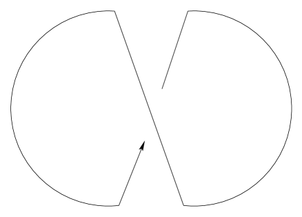
Figure 1: A center vortex with writhe

For physical center vortices, where Dirac strings turn into fat tubes of magnetic flux, the same picture holds, although for different reasons. For such fat tubes, the standard integrals for $Tw$ and $Wr$ are modified, and there is no sharp distinction between twist and writhe co95 . The modified integrals depend on the details of the mechanism that fattens the flux tubes (which may be thought of as the generation of a dynamical mass by quantum effects arising from infrared instability of the YM theory). There is no reason for $Tw$ or $Wr$ to be integers, or even fractions such as $1/2$. In physics language, $Tw$ and $Wr$ are dependent on collective coordinates of the vortex. So the situation should be somewhat similar to that for sphalerons.

If CS numbers can take on arbitrary values, how can $d=4$ topological charge, which is the difference of CS numbers, be restricted to integral values? The answer, of course, is $d=4$ compactness, which is not related to $d=3$ compactness; a non-compact $d=4$ space may have only compact $d=3$ cross-sections. Compactness in $d=4$ constrains the CS numbers whose difference is the topological charge, so that not every pair of $d=3$ condensates of CS number can occur in a compact $d=4$ space. We give some simple examples, analogous to the pairing of crossings (sphalerons) in a compact $d=3$ space, to show how these constraints arise. These examples interpret the net change in CS number as arising from a dynamic reconnection process, in which center vortices change their link number; only certain kinds of dynamic reconnection are allowed by compactness. The point of reconnection, when two otherwise distinct vortices have a common point, is simply the point of intersection of center vortices in the previously-studied picture of $d=4$ topological charge as an intersection number of closed vortex surfaces (plus linkages of these surfaces with nexus world lines) er00 ; co00 ; co02 ; such intersection points come in pairs for compact vortex surfaces.

We summarize our results as follows:

1. Even if compactification is not assumed a priori, and solitons possess collective coordinates amounting to arbitrary $N_{CS}$ for every soliton, the lowest-energy candidate vacuum state of a YMCS theory is one which is compact. The energetic favorability of compactification we describe by dynamical compactification.

2. There is no evidence for strings that locally bind sphalerons into paired objects; instead, there is evidence for a domain-wall “sphaleron” carrying half-integral CS number if the bulk sphalerons also carry half-integral CS number.

3. Sphalerons can be mapped onto over- and under-crossings of knots occuring in closed fictitious Abelian field lines associated with the non-Abelian CS term. There is always an even number of crossings for compact knots, and so an odd number of crossings of closed knot components must be compensated by an odd number of crossings elsewhere. The domain-wall sphaleron acts as a superconducting wall that confines the closed fictitious field lines to a compact domain, where they must close and have an integral CS number.

4. Fat self-linked center vortices can also carry arbitrary $N_{CS}$ associated with collective coordinates; we expect phenomena similar to those found for sphalerons.

5. For a compact $d=4$ condensate of center vortices and nexuses, living in the product of a $d=3$ space and a (Euclidean) “time” variable, possible time-dependent reconnection of vortices that would change link numbers is constrained by compactness to yield integral topological charge.

6. If fermions are added, we show that half-integral fermion number and half-integral CS number go together, and identify an extra fermion number of $1/2$ with a fermion zero mode at infinity, which is a zero mode of the domain-wall sphaleron at infinity. This result generalizes to the case of arbitrary CS number as well.

7. In the GGCS model, strings exist that bind TP monopoles to TP anti-monopoles and restore compactification; these strings are essentially those of center vortices, while the TP monopoles are like nexuses.

II Solitons in YMCS theory

In this section we establish notation, review the properties of solitons with the usual spherical ansatz in massive YMCS theory, and remark that every configuration in the functional integral for YMCS theory has a conjugate related by a Euclidean CPT-like transformation.

II.1 Spherically-symmetric solitons of YMCS theory

The action of YMCS is complex, so its classical solitons can be complex too. Then the CS action $I_{CS}$ defined in Eq. (4) below may be complex, and its real part is not interpretable as a CS number. We will always define $Im\;I_{CS}=2\pi kN_{CS}$, where the integer $k$ is the CS level. In general a large gauge transformation only changes the imaginary part of $I_{CS}$, and so this identification makes sense. But one may also ask whether it makes sense at all to discuss complex solitons as extrema of the action; certainly, as Pisarski pis points out, this is quite wrong in some circumstances. The other possibility is to use only solitons of the real part of the action, and simply evaluate the CS term at these solitons. Of course, this works fine in $d=4$, where the theta term adds nothing to the equations of motion. Ref. co96 argues that in YMCS there is a complex (but self-conjugate) spherically-symmetric soliton much like a sphaleron; the particular case studied there had purely real CS action and hence no CS number. We show here that the would-be sphaleron of Ref. co96 can easily be promoted to a sphaleron with $N_{CS}$= $1/2$.

One knows co82 ; chk that with no CS term, $d=3$ YM theory with no matter terms is infrared-unstable and non-perturbative, requiring the dynamical generation of a gluon mass $M$ of order $Ng^{2}$ for gauge group $SU(N)$, where $g$ is the gauge coupling. If this theory is extended to YMCS theory, it appears (at least from one-loop calculations co96 ) that the Chern-Simons gauge-boson mass $m=kg^{2}/4\pi$ is too small to cure the infrared instability, and so generation of dynamical mass is still required. The estimates of the critical level $k_{c}$ are based on one-loop calculations of the gauge-invariant pinch-technique (PT) gauge-boson propagator co82 ; chk ; cp ; papa and may not be very accurate, but unpublished estimates of two-loop corrections by one of us (JMC) suggest that the existence of a finite $k_{c}$ is well-established. The one-loop calculations give $k_{c}\simeq 2-5$ for $SU(2)$. The generation of a dynamical mass generally leads to confinement, via the creation of a condensate of center vortices th78 ; co79 ; mp ; no and nexuses co98 ; co99 ; er00 ; co00 ; cpvz ; bvz . The long-range effects essential for confinement come from pure-gauge parts that disorder the Wilson loop (i. e., give it an area law) by fluctuations in the Gauss linking number of vortices and the Wilson loop.

Define the usual anti-Hermitean $SU(2)$ gauge-potential matrix with the gauge coupling $g$ incorporated by:

$$A_{j}(\vec{x})=(\frac{g}{2i})\tau_{a}A_{j}^{a}(\vec{x})$$ (2)

where the component form $A_{j}^{a}(\vec{x})$ is the canonical gauge potential. The Euclidean YM action is:

$$I_{YM}=\int d^{3}x\frac{-1}{2g^{2}}TrG_{ij}^{2}.$$ (3)

To this can be added the Chern-Simons action:

$$I_{CS}=(2\pi ik)Q_{CS};\;\;Q_{CS}=\frac{-1}{8\pi^{2}}\int d^{3}x\epsilon_{ijk}Tr[A_{i}\partial_{j}A_{k}+\frac{2}{3}A_{i}A_{j}A_{k}].$$ (4)

The sum $I_{YM}+I_{CS}$ is the YMCS action $I_{YMCS}$. Throughout this paper we will define the CS number $N_{CS}$ as the real part of the integral in Eq. 4:

$$N_{CS}\equiv Re\;Q_{CS}=\frac{Im\;I_{CS}}{2\pi k}.$$ (5)

It is only from this real part that phase or gauge-invariance problems can arise. Gauge invariance under large (compact) gauge transformations requires that the Chern-Simons level $k$ is an integer, so that the integrand $\exp-I_{CS}$ of the partition function is unchanged. At the classical level, all gauge bosons acquire a Chern-Simons mass $m\equiv kg^{2}/4\pi$.

As mentioned in the introduction, the CS mass may not be large enough to cure the infrared instabilities of YMCS with no matter fields, and a dynamical mass is generated. This mass is the same for all gauge bosons. The infrared-effective action for this dynamical mass co82 is just a gauged non-linear sigma model:

$$I_{M}=\frac{-m^{2}}{g^{2}}\int d^{3}xTr[U^{-1}D_{i}U]^{2};\;\;D_{i}=\partial_{i}+A_{i};\;\;U=\exp(i\omega_{a}\tau_{a}/2).$$ (6)

When the unitary matrix $U$ and the gauge potential have the following gauge-transformation laws, the action $I_{M}$ is gauge-invariant:

$$U\rightarrow VU;\;\;A_{i}\rightarrow VA_{i}V^{-1}+V\partial_{i}V^{-1}.$$ (7)

The effective action $I_{eff}\equiv I_{YMCS}+I_{M}$ is valid in the infrared regime, but at large momentum $p$ or short distance $x$ the dynamical mass $m^{2}$ necessarily vanishes at a rate $\sim p^{-2}$ or $x^{2}$ (modulo logarithms). This dynamical-mass effective action is the same, for our purposes, as if one added a fundamental Higgs field, as in the Weinberg electroweak action.

Because the action is complex, in general we must deal with complex values for the gauge potentials and matter fields. However, the matrix $U$ must always be an $SU(2)$ matrix; that is, in the component form $U=\exp(i\tau_{a}\omega_{a}/2)$ the fields $\omega_{a}$ are always real.

II.2 Complex field configurations

With a complex action, there is no reason to restrict the path integral to real fields. There is an elementary theorem, essentially a Euclidean CPT theorem, applicable to complex YMCS gauge fields and any scalar fields, such as the fields $\psi(x)$ of the GG model discussed later. Given any configuration of gauge and scalar fields for which the actions evaluated on this configuration have the values $I_{YM},I_{CS},I_{M},I_{GG}$, we define a conjugate configuration by:

$$CPT:\;\;A_{i}(x),G_{ij}(x),U(x),\psi(x)\rightarrow A^{\dagger}(-x),-G_{ij}^{\dagger}(-x),U(-x),\pm\psi(-x)^{\dagger}$$ (8)

or in component language:

$$A_{i}^{a}(x)\rightarrow-A_{i}^{a}(-x)^{*},\omega_{a}(x)\rightarrow\omega_{a}(-x),\phi_{a}(x)\rightarrow\mp\phi_{a}(-x)^{*}.$$ (9)

The possible sign change of the scalar field $\psi$ reflects any intrinsic parity. Then the CPT-transformed configuration has actions $I^{*}$, $I_{CS}^{*}$, $I_{M}^{*}$, and $I_{GG}^{*}$. Note that $N_{CS}$ changes sign under conjugation.

Below we will look for solitons of the YMCS action plus matter terms. Generally these solitons, like the action itself, will be complex. They can be divided into two types: 1) those configurations that transform into themselves under CPT, which we call self-conjugate, and 2) those that transform to another configuration. Self-conjugate configurations have real action, including the CS term. It is easy to see that if any configuration of type 2) satisfies the complex equations of motion then so does its CPT conjugate, and both are admissible solitons if either is. Examples of type 1) solitons are given in co96 , for the YMCS action with dynamical mass generation. These solitons cannot be said to possess topological properties as expressed through the CS term, since the CS number $N_{CS}$ vanishes. However, from this self-conjugate soliton it is easy to generate solitons that are not self-conjugate with any desired CS number.

We review the sphaleron-like complex soliton co96 of the action $I_{YMCS}+I_{M}$ (see equations (3, 6)). Using the notation of co96 , a spherical soliton is described by four functions of $r$:

$$2iA_{i}=\epsilon_{iak}\tau_{a}\hat{x}_{k}(\frac{\phi_{1}(r)-1}{r})-(\tau_{i}-\hat{x}_{i}\hat{x}\cdot\vec{\tau})\frac{\phi_{2}(r)}{r}+\hat{x}_{i}\hat{x}\cdot\vec{\tau}H_{1}(r),$$ (10)

$$U=\exp(i\beta(r)\frac{\vec{\tau}\cdot\hat{x}}{2}).$$ (11)

The equations of motion, found by varying both $A_{i}$ and $U$, are:

$$0=(\phi_{1}^{\prime}-H_{1}\phi_{2})^{\prime}+\frac{1}{r^{2}}\phi_{1}(1-\phi_{1}^{2}-\phi_{2}^{2})+(im-H_{1})(\phi_{2}^{\prime}+H_{1}\phi_{1})-M^{2}(\phi_{1}-\cos\beta);$$ (12)

$$0=(\phi_{2}^{\prime}+H_{1}\phi_{1})^{\prime}+\frac{1}{r^{2}}\phi_{2}(1-\phi_{i}^{2}-\phi_{2}^{2})-(im-H_{1})(\phi_{1}^{\prime}-H_{1}\phi_{2})-M^{2}(\phi_{2}+\sin\beta);$$ (13)

$$0=\phi_{1}\phi_{2}^{\prime}-\phi_{2}\phi_{1}^{\prime}+H_{1}(\phi_{1}^{2}+\phi_{2}^{2})+(im(1-\phi_{1}^{2}-\phi_{2}^{2})+\frac{1}{2}M^{2}r^{2}(H_{1}-\beta^{\prime});$$ (14)

$$0=\frac{1}{r^{2}}[r^{2}(\beta^{\prime}-H_{1})]^{\prime}-\frac{2}{r^{2}}(\phi_{1}\sin\beta+\phi_{2}\cos\beta)$$ (15)

where

$$m=\frac{kg^{2}}{4\pi}$$ (16)

is the Chern-Simons mass at level $k$ and the prime signifies differentiation with respect to $r$. These equations reduce to those of co96 at $\beta=\pi$. As in co96 , Eq. (15), which is the variational equation for $U$, is not independent of the other three equations. It can be derived from them by simple manipulations because there is still an Abelian gauge degree of freedom:

$$\phi_{1}(r)\rightarrow\phi_{1}(r)\cos\alpha(r)+\phi_{2}(r)\sin\alpha(r) \phi_{2}(r)\rightarrow\phi_{2}(r)\cos\alpha(r)-\phi_{1}(r)\sin\alpha(r)$$ (17)

$$\beta(r)\rightarrow\beta(r)+\alpha(r) H_{1}(r)\rightarrow H_{1}(r)+\alpha^{\prime}(r).$$ (18)

The boundary conditions are:

$$r=0: \phi_{1}(0)=1;\;\;\phi_{2}(0)=H_{1}(0)=\beta(0)=0;$$ (19)

$$r=\infty: \;\;\phi_{1}(\infty)=\cos\beta(\infty);\;\;\phi_{2}(\infty)=-\sin\beta(\infty).$$

First consider the case $\beta=\pi$. Then co96 there is a solution where $\phi_{1}$ is real and $\phi_{2}$ and $H_{1}$ are pure imaginary. This corresponds to a self-conjugate soliton, so the CS action is purely real (that is, the CS integral $Q_{CS}$ in Eq. (4) is pure imaginary). This is easily checked from the explicit form

$$Q_{CS}=\frac{1}{8\pi^{2}}\int\frac{d^{3}x}{r^{2}}[\phi_{1}\phi_{2}^{\prime}-\phi_{2}\phi_{1}^{\prime}-\phi_{2}^{\prime}-H_{1}(1-\phi_{1}^{2}-\phi_{2}^{2})].$$ (20)

If any solution of the equations of motion is gauge-transformed as in Eq. (17), it remains a solution to these equations and all contributions to the action are unchanged except, of course, for the CS part of the action. If we start with the self-conjugate soliton above, and transform it with a function $\alpha(r)$ such that $\alpha(0)=-\pi,\;\alpha(\infty)=0$ one sees that the soliton is no longer self-conjugate, and in general all three functions $\phi_{1,2},\;H_{1}$ are complex. This choice of boundary conditions for $\alpha$ removes an integrable singularity in the original self-conjugate sphaleron, but does not change the YM and mass parts of the action. The change in the CS integral, because it does not affect the equations of motion, is necessarily a surface term:

$$\delta Q_{CS}=\frac{1}{2\pi}\left[\alpha(r)-\sin\alpha(r)\right|_{0}^{\infty}=\frac{1}{2}.$$ (21)

The new sphaleron has $N_{CS}=1/2$, as appropriate for a sphaleron.

The immediate objection is that one could as well choose any value for $\alpha(\infty)$, and change the sphaleron’s CS number to any desired value. Integration over this collective coordinate might cause sphalerons to be confined in pairs (as argued in ahps for TP monopoles in the GGCS model). However, it does not quite happen that way for sphalerons. We next show that integrating over $\alpha(\infty)$ for all sphalerons does increase the free energy, but does not lead immediately to confinement of sphalerons in pairs. In such a case, compactification becomes the preferred state dynamically.

III Dynamical compactification

As discussed in the introduction, sphalerons (and center vortices) present a challenge to the usual view of compact YMCS, since these solitons in isolation violate compactness and lead to problems with gauge invariance. In this section we consider several cases, beginning with the internally-inconsistent but instructive case in which $k$ is integral and only compact gauge transformations area allowed but there is a condensate of (non-compact) sphalerons. For odd $k$ the energy density of the vacuum is changed in sign from the case of even $k$, which raises the vacuum energy by an infinite amount. In the next case, $k$ is still an integer but we allow large gauge transformations of the form $\exp[i\vec{\tau}\cdot\hat{r}\alpha(r)/2]$ with arbitrary $\alpha(\infty)$. Since the action of a sphaleron depends on $\alpha(r)$ only through the CS phase factor, this variable can be treated as a collective coordinate and integrated over. We will see that this integral again raises the free energy, suggesting that the compactified theory is preferred on energetic grounds. Finally, we consider the case of general $k$, including spatially-variable $k$, and non-compact gauge transformations and find, analogous to Lüscher’s work lus in $d=4$, that if $k$ takes on a non-integral value in a bounded domain and an integral value outside it, this domain or “bag” has a positive energy, scaling with the bag volume, above the integral-$k$ vacuum.

This last case gives us a clue to what actually causes the ostensibly non-compact theory to compactify. We find no evidence for strings that would join pairs of sphalerons together, nor do the collective coordinate integrations reduce the theory to the zero-sphaleron sector. Instead, we argue in Sec. IV that among the collective coordinates for large gauge transformations with any value of $\alpha(\infty)$, there is the possibility of formation of a domain-wall sphaleron that places half-integral CS number on a closed surface surrounding an odd number of sphalerons, to add to the half-integral CS number present from the sphalerons inside. This domain wall itself has no energy, and is a pure-gauge object; it can be moved around, deformed, and so on, without changing the physics. It acts as a superconducting wall that causes the fictitious Abelian field lines associated with non-Abelian CS number to be confined to the interior of the domain wall, or in other words to be compact.

Our arguments are based on the assumption that a condensate of sphalerons in YMCS theory can be treated in the dilute-gas approximation, or equivalently that all solitons are essentially independent. When a CS term is present in the action, the partition function $Z$ is the usual expansion as a sum over sectors of different sphaleron number:

$$Z(k)=\sum_{J}Z_{J};\;\;Z_{J}(k)=\sum_{c.c.}\frac{1}{J!}e^{-\sum I_{c}}+\dots$$ (22)

where $Z_{J}(k)$ is the partition function in the sector with $J$ sphalerons; the subscript $c.c.$ indicates a sum over collective coordinates of the sphalerons; $I_{c}$ is the action (including CS action) of a sphaleron and the omitted terms indicate corrections to the dilute-gas approximation. To be more explicit, we separate the sum over collective coordinates into kinematic coordinates, such as spatial position, and gauge collective coordinates. The former we represent in the standard dilute-gas way and the latter we indicate as a functional integral over large gauge transformations $U$:

$$Z(k)=\int(dU)\sum\frac{1}{J!}(\frac{V}{V_{c}})^{J}\exp-\{JRe\;I_{c}+2\pi ik[JN_{CS}(A_{c})+N_{CS}(U)]\}$$ (23)

Here $Re\;I_{c}$ is the real part of the action, $N_{CS}(A_{c})$ is the CS number of each individual soliton of gauge potential $A_{c}$ (taken in some convenient gauge), and $N_{CS}(U)$ is the CS number of the large gauge transformation. As in Sec. II, we choose $A_{c}$ so that $N_{CS}(A_{c})=0$.

If we now restrict the large gauge transformations $U$ to be compact, so that $N_{CS}(U)=K$, an integer, we recover the standard djt result that $Z(k)$ is non-zero only for $k$ an integer.

Now retain the assumption that only compact gauge transformations are allowed and that $k$ is integral, but allow a condensate of sphalerons. Sphalerons correspond to a limitation of $\alpha(a;\infty)$ to the two values $\pm\pi$. The $\sin\alpha$ term vanishes in Eq. (21), and the collective-coordinate sum reduces to:

$$Z=\sum_{J_{+},J_{-}}\frac{1}{J_{+}!J_{-}!}(\frac{V}{V_{c}})^{J}\exp-[JRe\;I_{c}]e^{ik\pi(J_{+}-J_{-})}=\exp\{e^{i\pi k}2(\frac{V}{V_{c}})\exp-[Re\;I_{c}]\};\;\;(J=J_{+}+J_{-}).$$ (24)

If $k$ is odd, this expression for $Z$ has precisely the opposite sign in the exponent to that of a normal dilute-gas condensate, which means that the free energy, which for a normal dilute-gas condensate is negative, has turned positive. So the non-compactified theory has in a higher free energy than the compactified theory. (Non-compactification also leads to a number of other unphysical results in the dilute-gas approximation, which we will not dwell on here.)

Now consider the case of non-compact gauge transformations. Suppose that, as in Sec. II, the sphalerons are obtained by a gauge transformation of the form given in Eq. (17) acting on a self-conjugate soliton, whose action is real and positive. The $a^{th}$ soliton is at position $\vec{r}-\vec{a}\equiv\vec{r}(a)$. Denote by $\alpha(a;\infty)$ the asymptotic value of the gauge variable for the $a^{th}$ soliton. Since the total CS number of all $J$ sphalerons comes from a surface contribution, we can immediately write the phase factor in the action by generalizing Eq. (21):

$$Z(k)=\sum_{J}\frac{1}{J!}(\frac{V}{V_{c}})^{J}\exp-[JRe\;I_{c}]\exp ik[\alpha-\sin\alpha]$$ (25)

where

$$\alpha=\sum_{a=1}^{J}\alpha(a;\infty).$$ (26)

We are treating the $\alpha(a;\infty)$ as collective coordinates, so we integrate over them:

$$Z(k)=\sum_{J}Z_{RJ}\times\{\prod_{a}\int_{0}^{2\pi}\frac{d\alpha(a;\infty)}{2\pi}\}\exp ik[\alpha-\sin\alpha]$$ (27)

where $Z_{RJ}$ indicates the explicitly real terms in the summand of Eq. (25). This integral is reduced to a product by using the familiar Bessel identity

$$e^{iz\sin\theta}\equiv\sum_{-\infty}^{\infty}J_{N}(z)e^{iN\theta}$$ (28)

with the result, for integral $k$, $[J_{k}(k)]^{J}$. So the dilute-gas partition function is:

$$Z(k)=\sum_{J}\frac{1}{J!}(\frac{V}{V_{c}})^{J}\exp J[-Re\;I_{c}+\ln J_{k}(k)]=\exp\{\frac{V}{V_{c}}e^{-Re\;I_{c}}J_{k}(k)\}.$$ (29)

Since $1\geq J_{k}(k)>0$ for all levels $k$, we see that integrating over the collective coordinates has increased the free energy (the negative logarithm of $Z$). This suggests that by properly compactifying the sphalerons, so that the gauge behavior at infinity is under control, we will lower the free energy, yielding something like the usual dilute-gas partition function (which is Eq. (29) without the $J_{k}(k)$ factor).

Once one allows non-compact gauge transformations one might as well allow non-integral $k$. The results are analogous to those found long ago by Lüscher lus for $d=2$ $CP^{N}$ models and $d=4$ gauge theory with instantons and a $\theta$ angle. Of course, the calculations for non-integral $k$ only make sense in the non-compact case. For non-integral $k$ the function $J_{k}(k)$ of Eq. (29) must be replaced by

$$F(k)=\sum_{-\infty}^{\infty}J_{N}(k)\frac{\sin[\pi(k-N)]}{\pi(k-N)}.$$ (30)

This reduces to $J_{k}(k)$ for integral $k$.

We promote $k$ to an axionic field $k(x)$ and put it under the integral sign in the CS action of Eq. (4). Take $k(x)$ to vanish outside some closed surface and to have a constant non-integral value $k$ inside (except for some thin-wall transition region). To follow Lüscher, we consider the expectation value of $\exp I_{CS}$ in a YM theory, which is the same as $Z(k)/Z(0)$ of YMCS theory. This result is given by replacing $J_{k}(k)$ in Eq. (29) with $F_{k}(k)$ from Eq. (30). Because djt the CS integral is a surface integral for the pure-gauge configurations over which we are integrating, we have:

$$\langle e^{2\pi ikN_{CS}}\rangle_{YM}=\langle e^{2\pi ik\oint_{S}dS_{i}V_{i}}\rangle$$ (31)

and:

$$\langle e^{2\pi ikN_{CS}}\rangle_{YM}=\frac{Z(k)}{Z(0)}=\exp\{\frac{V_{S}}{V_{c}}e^{-I_{c}}[F(k)-1]\}$$ (32)

where $V_{S}$ is the volume enclosed by the surface $S$ and $V_{i}$ is a CS surface density (given explicitly for sphaleron-like configurations in Eq. (47) below). Because $F(k)\leq 1$, there is an interpretation similar to Lüscher’s: There is a bag, defined by the surface where $k(x)$ changes, with an energy above the vacuum by an amount proportional to the volume of the bag. This bag is analogous to the domain-wall sphaleron discussed in the next section.

Some qualitative information about the CS susceptibility can be gleaned from the small-$k$ limit of Eq. (32). In this limit,

$$F(k)\rightarrow 1-k^{2}(\frac{2\pi^{2}-9}{12})\equiv 1-\gamma k^{2}.$$ (33)

This form of the small-$k$ limit allows us to interpret the distribution of $N_{CS}$ as Gaussian:

$$\langle e^{2\pi ikN_{CS}}\rangle_{YM}\rightarrow\exp-\{2\pi^{2}k^{2}\langle N_{CS}^{2}\rangle\}.$$ (34)

Because we expect $\langle N_{CS}^{2}\rangle\sim V$, the Gaussian expectation value vanishes in the infinite-volume limit. In fact, by comparing Eqs. (32) and (34) we find an approximate value for the CS susceptibility:

$$\frac{\langle N_{CS}^{2}\rangle}{V}=\frac{\gamma}{2\pi^{2}V_{c}}e^{-I_{c}}.$$ (35)

This expression, while presumably not quantitatively accurate, is of a form suggested earlier cy in which the $d=3$ topological susceptibility is of the form

$$\frac{\langle N_{CS}^{2}\rangle}{V}=\xi\langle\Theta\rangle$$ (36)

where $\Theta$ is the trace of the stress-energy tensor and $\xi$ is a numerical constant. For a dilute gas condensate,

$$\frac{1}{3}\langle\Theta\rangle=\frac{1}{V_{c}}e^{-I_{c}}$$ (37)

and $\xi=\gamma/6\pi^{2}$ from Eq. (35).

IV Sphalerons and half-integral knots

A sphaleron has CS number $1/2$. If sphalerons are dilute, they can be idealized to pure-gauge configurations. These configurations can be associated with fictitious Abelian field lines through the Hopf fibration $S^{3}\rightarrow S^{2}$, with homotopy $\Pi_{3}(S^{2})\simeq Z$. The integer classes of this homotopy come from an integral, the Hopf invariant, which is in fact the same as the original CS number (see, eg , jahn ; jp ; co02 ). The Hopf invariant $N_{H}$ is both a Gauss link number for the pre-images of any two distinct points in $S^{2}$ in the Hopf fibration, and an Abelian CS term for a fictitious Abelian gauge potential and magnetic field. Pre-images of $S^{2}$, necessarily closed curves, are just field lines of this fictitious magnetic field, and so the Hopf invariant expresses the linking of any two distinct closed field lines. (For idealized Dirac-string center vortices the CS number can also be expressed equivalently as a Gauss link integral and as an Abelian CS term, but the normalization is different, and the CS number can be half-integral in the simplest case.)

For the sphaleron the CS number is $1/2$; how can this be reconciled with the link-number interpretation? The answer is that in knot theory knots presented as two-dimensional graphs with over- and under-crossings, each crossing contributes $\pm 1/2$ to the total link number, just as does an isolated sphaleron. In a certain sense, which we make explicit below, sphalerons can be mapped onto these crossings. Compact knots must have an even number of crossings; only knots stretching to (and thus closed at) infinity can have an odd number of crossings in a region excluding infinity. So the sphaleron puzzle comes down to how one closes the fictitious Abelian flux lines that flow through the sphaleron. We show here how this can be done by introducing a domain-wall sphaleron containing the other $1/2$ needed for integral CS number, and hence integral Hopf invariant. The domain wall can be, but is not required to be, on the sphere at infinity. If not, then the fictitious Abelian field lines vanish identically outside the domain wall, which acts as a superconducting wall for the fictitious field lines.

We give a second interpretation of the field-line knots, which relates them to the formulation of $d=4$ topological charge as the intersection of closed vortex and vortex-nexus surfaces. This interpretation maps the $d=4$ intersection numbers onto $d=2$ intersection numbers of closed lines (vortices) in the two-plane, some of which must carry point nexuses and anti-nexuses. In a formal sense, the resulting formulation of half-integral CS number becomes a two-dimensional projection of earlier formulas er00 ; co00 which express $d=4$ $SU(2)$ topological charge as composed of components of charge $\pm 1/2$, localized at the (assumed transverse) intersection points of $d=4$ vortices and vortex-nexus combinations. The total (and integral) topological charge is computed as an intersection integral with an extra weight factor coming from traces over the Lie-algebra matrices of vortices and nexuses. Both interpretations will illustrate how an odd number of sphalerons requires a sphaleron-like configurations at infinity.

IV.1 Sphalerons and link numbers of knots

The connection between the non-Abelian CS number of a pure-gauge configuration $U$ and the Abelian linking number is found (see, for example, jp ; jahn ; co00 ) by exploiting the Hopf map $S^{3}\rightarrow S^{2}$, with homotopy $\Pi_{3}(S^{2})\simeq Z$, in the form of a map from the $SU(2)$ group element to a unit vector $\hat{n}$:

$$U\tau_{3}U^{-1}\equiv\tau\cdot\hat{n}.$$ (38)

This is, of course, a compact map. Since $U$ can be right-multiplied by $\exp(i\alpha\tau_{3}/2)$ without changing $\hat{n}$, each $\hat{n}$ corresponds to a coset $SU(2)/U(1)$. The linked curves in question are the pre-images of points $\hat{n}$ on the sphere $S^{2}$. This unit vector defines an Abelian gauge potential and field, via:

$${\mathcal{A}}_{i}=iTr(\tau_{3}U\partial_{i}U^{-1});\$$ (39)

$${\mathcal{B}}_{i}=-i\epsilon_{ijk}Tr(\tau_{3}U\partial_{j}U^{-1}U\partial_{k}U^{-1})=\frac{1}{2}\epsilon_{ijk}\epsilon_{abc}n^{a}\partial_{j}n^{b}\partial_{k}n^{c}.$$ (40)

Because of the properties of the $\epsilon$ symbol and of group traces, the non-Abelian CS integral of Eq. (5) can be written in terms of the Abelian field and potential:

$$N_{CS}=\frac{1}{16\pi^{2}}\int d^{3}x{\mathcal{A}}_{i}{\mathcal{B}}_{i}\equiv N_{H},$$ (41)

where $N_{H}$ is the Hopf invariant, an integer characterizing the homotopy class of the map. The second equation in (40) is only true if Dirac strings are omitted. For sphalerons no such strings occur (see Eq. (45) below).

The Hopf invariant is a link number of any two distinct field lines of the field ${\mathcal{B}}_{i}$. As textbooks on knot theory discuss knots , these $d=3$ knots can be expressed in a quasi-two-dimensional way, with graphs constructed from over- and under-crossings of components of knots, and topological invariance in $d=3$ reduced to Reidemeister moves in $d=2$. (Another good example of the $d=2$ nature of $d=3$ knots is Witten’s derivation wit89 of Jones polynomials from $d=2$ conformal field theory.) In this picture, knot components lie in a plane, except that they fail to intersect at an over- or under-crossing by a vanishingly small distance $\epsilon$. Of course, in $d=3$ linked knot components may be very far from touching one another, but in our case we are only interested in nearly-touching crossings, so that contributions to the Gauss link number are localized to these crossings. The global $d=3$ topology is not affected by this assumption. Then each crossing of distinct knot components contributes an additive term $\pm 1/2$ to the conventional Gauss linking integral, and there are no contributions from portions of the knot components separated by distances that are large compared to $\epsilon$. (As we discuss below, this contribution of $\pm 1/2$ also holds for self-crossings of one component with itself, leading to integral framed link number, because each self-crossing is actually a double crossing.) There is no contribution away from the crossings even if the knot components extend in an arbitrary way (as long as components do not cross each other) into all three dimensions. For closed compact components there is always an even number of crossings and hence an integral link number. Half-integral linking numbers occur naturally for non-compact knots, that is, knots with an odd number of crossings. For closed knot components, this can only occur when the component curves are closed at infinity.

We give a specific example of these concepts. A pure-gauge sphaleron centered at the origin is described by a gauge function $U$ of the form:

$$U=\exp[i\beta(r)\vec{\tau}\cdot\hat{r}/2];\;\;\beta(0)=0;\;\;\beta(\infty)=\pi.$$ (42)

One finds for the fictitious Abelian components:

$$\hat{n}=\hat{r}\cos\theta+\hat{\theta}\sin\theta\cos\beta+\hat{\phi}\sin\theta\sin\beta;$$ (43)

$${\mathcal{A}}_{i}=\hat{r}_{i}\beta^{\prime}\cos\theta+\frac{\hat{\phi}_{i}}{\rho}(\cos\beta-1)\sin^{2}\theta-\frac{\hat{\theta}_{i}}{r}\sin\theta\sin\beta;$$ (44)

$${\mathcal{B}}_{i}=\frac{2\hat{r}_{i}}{r^{2}}\cos\theta(\cos\beta-1)+\frac{\hat{\phi}_{i}}{r}\beta^{\prime}(1-\cos\beta)\sin\theta+\frac{\hat{\theta}_{i}}{r}\beta^{\prime}\sin\theta\sin\beta.$$ (45)

These field lines have several important properties. First, the flux integrated over any sphere surrounding the origin is zero, so there is no monopole and no Dirac string for this sphaleron. Second, by inspection of Eq. (45) one sees that there is one, and only one, way in which the field lines can be terminated in a finite region. If for $r\geq a$, $\beta(r)$ takes the value $2\pi N$ where $N$ is an integer, the field ${\mathcal{B}}_{i}$ vanishes identically for $r\geq a$. Since the fictitious field lines are closed, this can only happen if the field lines run along the surface of the sphere $r=a$ and at some point return to the vicinity of the sphaleron and close. Schematically, the field lines look like those depicted in Fig. 1. The bounding surface $r=a$ acts as a superconductor for the Abelian field lines. (Of course, this bounding surface need not literally be a sphere, but it can be any surface with the topology of $S^{2}$ that encloses the sphaleron.) Once the field lines are compactified in this way, there is no problem interpreting the Hopf invariant in terms of linkages of two of this family of closed curves. On the other hand, if $\beta(r)$ never reaches $2\pi N$, it is easy to see from the explicit form of Eq. (45) that the field lines never return to the vicinity of the sphaleron, but continue on to infinity.

A third important property is that in the vicinity of the sphaleron the field lines are sheared so that any two lines, projected into a plane, cross each other. Below we will interpret this crossing as a contribution to the linkage of knotted field lines.

For the sphaleron $\beta(r)$ approaches $\pi$ asymptotically. We can, in analogy with the discussion above, bring the radius at which $\beta=\pi$ to any desired finite value $r=b$, as long as $b$ is large compared to all natural length scales, such as $M^{-1}$. This does not compactify it, because its Abelian field lines keep on going past $r=b$. But we can compactify it with a domain-wall sphaleron at $r=a,\;a>b$, by increasing $\beta$ to $2\pi$ at $r=a$. Then, as shown, the fictitious field lines close, and there is an extra CS number of $1/2$ on the domain-wall sphaleron.

The CS number for the sphaleron can be found explicitly from the Hopf invariant integral Eq. (41):

$$N_{CS}=-\frac{1}{2\pi}[\beta(\infty)-\sin\beta(\infty)]=-\frac{1}{2}.$$ (46)

and of course it has the same value as would be obtained from the spherical ansatz form of Eq. (20). It can also be written as a surface integral:

$$N_{CS}=\int d^{2}S_{i}V_{i};\;\;V_{i}=-\frac{\hat{r}_{i}}{8\pi^{2}r^{2}}[\beta-\sin\beta].$$ (47)

Clearly, the contribution to $N_{CS}$ from the domain-wall sphaleron can also be written as a surface integral over the domain wall.

So what does a link number of $1/2$ mean for a sphaleron? Recall knots how link numbers can be written as a sum of terms, each of which is $\pm 1/2$. The knots are displayed with suitable over- and under-crossings in two-dimensional pictures. For each crossing point $p$ a factor $\epsilon(p)=\pm 1$ is defined as shown in Fig. 2.

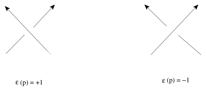
Figure 2: Over- and under-crossings and their values.

For two distinct curves the link number $Lk$ is then defined as:

$$Lk=\frac{1}{2}\sum_{p\in C}\epsilon(p)$$ (48)

where $C$ is the set of crossing points of one curve with the other (self-crossings will be discussed later). This suggests that in some sense a sphaleron is the topological equivalent of a single crossing, with (as one quickly checks) an even number of crossings needed for describing the linkage of closed compact curves. Of course, since a sphaleron is localized, one needs to interpret the crossings in Figs. 1 or 2 as being infinitesimally separated. This in itself is not necessary for understanding the topology but it is necessary for interpreting the topology in terms of localized sphalerons.

We can express this in terms of the sort of integral occurring in the formula (56) for link number. Consider the two infinite straight lines

$$z_{i}=(s\cos\alpha,s\sin\alpha,0);\;\;z^{\prime}_{i}=(t\cos\beta,t\sin\beta,\epsilon)$$ (49)

where $-\infty<s,t<\infty$ with $ds,dt$ the elements of distance along the lines. Their distance of closest approach is $\epsilon$. For a configuration of two infinite straight lines the value of $\epsilon$ does not matter, but if the lines are part of a knot with curvature, $\epsilon$ must be treated as infinitesimal. The integrals in the formula

$$Lk=\frac{1}{4\pi}\int^{\infty}_{-\infty}ds\int^{\infty}_{-\infty}dt\epsilon_{ijk}\dot{z}_{i}\dot{z}^{\prime}_{j}\frac{(z-z^{\prime})_{k}}{|z-z^{\prime}|^{3}}$$ (50)

are readily done, and yield:

$$Lk=\frac{1}{2}{\rm sgn}[\epsilon_{ijk}\dot{z}_{i}\dot{z}^{\prime}_{j}(z-z^{\prime})_{k}].$$ (51)

In the course of evaluating the integral of Eq. (50) in the limit $\epsilon\rightarrow$0, one encounters standard definitions of the Dirac delta function which allow one to write this integral for the link number as:

$$Lk=\frac{1}{2}\oint dz_{i}\oint dz^{\prime}_{j}\epsilon_{ij}\delta(z-z^{\prime}){\rm sgn}\;\epsilon$$ (52)

where ${\rm sgn}\;\epsilon$ refers to the sign of the distance shown in Eq. (49) by which the two components are separated out of the plane at their crossing points, that is, whether there is an overcrossing or an undercrossing.

As long as one presents the knots as being quasi-two-dimensional, which means that their components lie in one plane except for infinitesimal displacements into the third dimension for crossings, there are no other contributions to the integral for $Lk$, because the triple product in its definition vanishes for curves lying in a plane. As a result, in the present interpretation of link number, the link number can be thought of as being localized, in units of $1/2$, to points where the components of the knot appear to cross. This is quite similar to the interpretation in $d=4$ er00 ; co00 ; co02 of $SU(2)$ topological charge as occurring in localized units of $1/2$. The localization is associated with the intersection of surfaces representing center vortices and vortex-nexus combinations, with an analog in $d=2$ which we discuss below.

In fact, it is easy to see that away from the infinitesimally-close crossing points, the knots may be arbitrarily deformed into the third dimension as long as components do not cross each other, since the difference of the contribution to $Lk$ from a $d=2$ component and one deformed into $d=3$ is a Gauss integral with no linkages. If, in this process of deformation, other knot components become infinitesimally close to each other, new contributions to the total $Lk$ of $\pm 1/2$ will be generated, but their sum will be zero.

IV.2 Knots and $d=2$ intersection numbers

The form of Eq. (52) for the link number is very suggestive; aside from the sign function in the integrand and the factor of $1/2$, it is the integral representation of the signed sum of intersection numbers for curves lying in a plane. In $d=4$, the usual topological charge (the integral of $G\tilde{G}$) for idealized pure-gauge $SU(2)$ center vortices and nexuses is also represented by an intersection-number integral, including a factor of $\pm 1/2$ coming from group traces er00 ; co00 . The sign of this group factor is governed by the presence or absence of nexuses and anti-nexuses, each of which reverses the direction of the $SU(2)$ magnetic field lines lying in the vortex surface. In $d=4$ center vortices are described by closed two-surfaces, and nexus-vortex combinations are described by such surfaces with a closed nexus world line lying in the vortex surface. For every nexus world line there is an anti-nexus world line. The intersection-number form can be translated into a link-number form co00 , where the link is between a center vortex with no nexus and a nexus (or anti-nexus) world line.

Here we give some simple examples of $d=3$ knot linkages represented by $d=2$ graphs which can be considered as the projection into two dimensions of $d=4$ vortex-nexus topological charge. There is no need to distinguish over- and under-crossings; instead, the crossings are interpreted as intersections of closed lines whose orientation changes whenever a (point) nexus is crossed in the process of tracing out a closed line. The link number is calculated by counting (with signs) the linkages of closed curves and nexuses or anti-nexuses. In this case a curve and a point are linked if the point is inside the curve; otherwise they are unlinked.

We obtain the $d=2$ CS integral, which is completely analogous to the $d=4$ expression for center vortices and nexuses co00 :

$$N_{CS}=\sum_{\rm crossings}\oint dz_{i}\oint dz^{\prime}_{j}\epsilon_{ij}\delta(z-z^{\prime})Tr(QQ^{\prime})$$ (53)

where $Q,Q^{\prime}$ take on the values $\pm\tau_{3}/2$, with the sign depending on the orientation of segments of the closed curves. The orientation must change every time a nexus or anti-nexus is crossed in the course of tracing out the curve. Fig. 3 illustrates this formalism for a simple two-component knot represented both as an over/undercrossing link and as a vortex-nexus link. In the figure, a filled-in circle is a nexus and an open circle is an anti-nexus; there must be as many of one as of the other on any closed vortex curve. A more detailed discussion of the correspondence between knots and vortex-nexus ideas (including twist and writhe) will be given elsewhere.

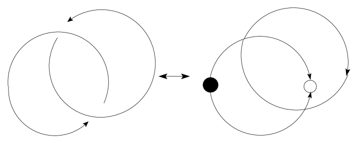
Figure 3: A simple knot presented as a $d=2$ projection of a center vortex and a center vortex with a nexus (filled circle) and anti-nexus (open circle).

In this way we can connect topological charges in dimensions two, three, and four. In all cases, for $SU(2)$ the localized unit of topological charge is $\pm 1/2$, but compactification of the space under consideration yields a sort of topological confinement of these fractional units to integral totals.

V Linked and writhing center vortices

The standard center vortex co79 is an Abelian configuration, essentially a Nielsen-Olesen vortex. It contributes to CS number through the $A\cdot B$ term, not through the $A^{3}$ term, and the techniques used above to generate an Abelian potential and field are irrelevant; the vortex itself is Abelian, and in its idealized pure-gauge version is described by a closed Dirac-string field line. These closed lines may be linked, including the self-linkages given in terms of twist and writhe. Such linkages generate CS number, as expressed through the $A\cdot B$ integral. However, even integral link numbers give rise to CS numbers whose quantum is $1/2$, while twist and writhe give rise to arbitrary real CS number.

Generically, two distinct center vortices in $d=3$ never touch each other, whether or not they are linked. But to generate $d=4$ topological charge, which is a weighted intersection integral of the points at which center vortices intersect (possibly with the intervention of nexuses), two vortex surfaces must have common points. If the intersection is transverse, these points are isolated. There must be a corresponding notion of linked vortices touching each other in $d=3$ as well. We can think of vortices as closed strings in $d=3$, which evolve in a Euclidean “time” variable (the fourth dimension). Vortices have points in common at the isolated instant in which they change their link number (reconnection) co95 . To generate topological charge, we must change the CS number, which is equivalent to changing the link number. Also necessary in this simple situation is the presence of at least one nexus, which reverses the sign of the vortex magnetic fields. We discuss some elementary cases in which reconnection changes the CS number by $\pm 1/2$, and in which, if compactness in $d=4$ is demanded, the overall change in link number yields integral topological charge. Note that compactness in $d=3$ has nothing to do with compactness in $d=4$ (consider the product $S^{3}\times R$). Even for reconnection that changes the writhe of a single vortex, which can be arbitrary, it is possible to have changes in CS number quantized in units of $1/2$. The appearance of this unit of $1/2$, plus the pairing of $d=4$ intersection points of compact surfaces er00 ; co00 ; co02 is somewhat analogous to the pairing of over- and under-crossings for compact $d=3$ knots, discussed above.

In considering the evolution in time of various field configurations carrying topological charge, note that there are real differences between $d=4$ topological charge interpolated by sphalerons and by reconnection of vortices. A sphaleron is the (unstable) saddlepoint of a classical path in configuration space. One can extend the sphaleron gauge angle $\beta(r)$ to a function $\beta(r,t)$ with $\beta(r,0)\equiv\pi$ and which yields unit topological charge in the form $(1/(2\pi)[\beta(r,\infty)-\beta(r,-\infty)]=1$, such as $\beta=2\arctan(r/t)$. There is no need to pair the sphaleron with another sphaleron. A vortex, however, cannot evolve classically since it must reconnect and overlap with itself or with another vortex. The action penalty from overlap yields a tunneling barrier, and thus reconnections with half-integral CS number must be paired.

It would take another paper to discuss all the ramifications of vortex self-linkage, including the role of nexuses, and the new twisted nexus presented recently co02 . We restrict ourselves here to a few simple examples, including a new Abelian twisted vortex, and some general conclusions. The main point is that self-linking, whether considered for idealized Dirac-string vortices or for fat physical vortices, leads to contributions to $N_{CS}$ that can be essentially arbitrary real numbers, although the self-linking is spatially localized. As for sphalerons, one can introduce a domain wall to carry extra CS number, bringing the total to an integer.

V.1 Linking of distinct vortices and half-integral CS number

For pure-gauge center vortices the interpretation of $N_{CS}$ in terms of a link number is straightforward, if two distinct vortices are linked, but more troublesome if self-linking is involved. For the straightforward case of linking of distinct vortices the CS number is half the link number and can therefore be half-integral. If it is half-integral, the configurations is not compact, even though the links composing the two vortices are spatially compact. If these links have maximum spatial scale $L$, the gauge potential from the vortices behaves as $L^{2}/r^{3}$ when $r\gg L$, and so it falls off sufficiently rapidly at large distances that no surface terms arise in various integrals of interest.

The gauge parts of two distinct center vortices are described by closed curves $\Gamma,\Gamma^{\prime}$:

$$A(x;\;\Gamma)_{i}=(\frac{2\pi\tau_{3}}{2i})\epsilon_{ijk}\partial_{j}\oint_{\Gamma}dz_{k}\Delta(x-z);$$ (54)

$$B(x;\;\Gamma^{\prime})_{i}=(\frac{2\pi\tau_{3}}{2i})\oint_{\Gamma^{\prime}}dz_{i}\delta(x-z)$$ (55)

where $\Delta(x-z)$ is the free massless propagator in $d=3$. The CS number of the mutual linkage of $\Gamma,\Gamma^{\prime}$ is:

$$N_{CS}=\int d^{3}xTrA(x;\;\Gamma)_{i}B(x;\;\Gamma^{\prime})_{i}=(\frac{-1}{2})Lk(\Gamma,\Gamma^{\prime});$$ (56)

$$Lk(\Gamma,\Gamma^{\prime})\equiv\oint dz_{i}\oint dz^{\prime}_{j}\epsilon_{ijk}\partial_{k}\Delta(z-z^{\prime}).$$ (57)

If curves $\Gamma,\Gamma^{\prime}$ are linked, as in Fig. 4, the corresponding CS number is $1/2$, because of the factor $1/2$ in front of the $Lk$ integral in Eq. (56).

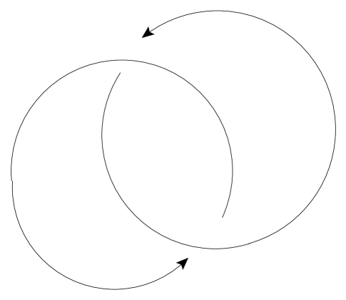
Figure 4: A simple two-component knot with no twist or writhe.

V.2 Self-linkage of Dirac-string vortices

Self-crossings of a single vortex Dirac string give rise to twist ($Tw$) or writhe ($Wr$). With the usual sort of ribbon framing knots used to define self-crossings, neither twist nor writhe is a topological invariant and neither is restricted to integral values. Their sum, the framed link number $FLk$, is an integer-valued topological invariant whose value depends on the framing. A simple ribbon-framing is shown in Fig. 5. The CS number is not the integer $FLk$; instead, it is the writhe $Wr$, or self-link integral, given in Eq. (60) below.

Because the vortex is Abelian, $N_{CS}$ receives contributions only from the $\vec{A}\cdot\vec{B}$ term co95 ; cy :

$$N_{CS}=\frac{-1}{8\pi^{2}}\int d^{3}xTr\vec{A}\cdot\vec{B}=\frac{1}{4}Lk(\Gamma,\Gamma)$$ (58)

where $Lk(\Gamma,\Gamma)\equiv Wr$ is the self-linking number or writhe of Eq. (60). The writhe can be anything, depending on the geometry of the vortex.

For Frenet-Serret framing (displacing the ribbon infinitesimally from the curve $\Gamma$ along the principal normal vector $\hat{e}_{2}$) the twist is:

$$Tw=\frac{1}{2\pi}\oint ds\hat{e}_{2}\cdot\frac{d\hat{e}_{3}}{ds}$$ (59)

where $\hat{e}_{3}$ is the binormal vector. It too is geometry-dependent and not restricted to be an integer or simple fraction.

A typical self-crossing is shown in Fig. 1, which was introduced to illustrate a center vortex. We now interpret that figure as a picture of twisting but unwrithed fictitious Abelian field lines (the discussion is essentially the same if one replaces “twist” by “writhe”; the two are interconvertible). Even though this is a compact knot, it appears that there is only one crossing. Actually there are two for the framed knot of Fig. 5. For an untwisted curve the Gauss link number for the writhing curve $\Gamma$ is equal to the writhe:

$$FLk(\Gamma,\Gamma)=Wr=\frac{1}{4\pi}\oint_{\Gamma}dz_{i}\oint_{\Gamma}dz^{\prime}_{j}\epsilon_{ijk}\frac{(z-z^{\prime})_{k}}{|z-z^{\prime}|^{3}}.$$ (60)

As the contours are traced out the crossing point is encountered twice, so the value of $FLk$ in Eq. (60) is $(1/2)+(1/2)=1$. Or one may calculate $FLk$ by counting the crossings of the link with its ribbon frame; again there are two crossings.

Note that the same value of the writhe applies to the center vortex of Fig. 1, but because of group traces the CS number is, for gauge group $SU(2)$, half the writhe. We see that topologically a unit of writhe in the fictitious Abelian field lines corresponds to two sphalerons, but a unit of writhe in a center vortex corresponds to only one sphaleron.

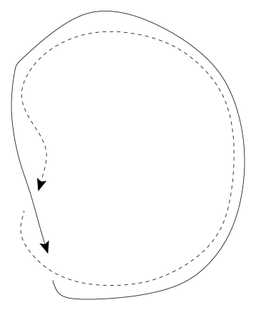
Figure 5: Ribbon framing of a single-component knot with one unit of twist and two crossings.

We note that the self-linking number of a pure-gauge center vortex, as described in Eq. (54), is also the self-flux of the corresponding Abelian potential of Eq. (39):

$$Lk(\Gamma,\Gamma)=Wr=\frac{1}{8\pi}\oint_{\Gamma}dz_{i}{\mathcal{A}}_{i}(z).$$ (61)

The simplest case of dynamic reconnection of a center vortex begins with a configuration such as that shown in Fig. 1, to which we assign some twist $Tw$ and writhe $Wr$, whose sum is an integer, the framed link number. Reconnection, which changes the overcrossing shown in the figure to an undercrossing, changes the framed link number by 2, not 1, as one can appreciate from a study of Fig. 5. If we assume that the lines shown in Fig. 1 are separated by an infinitesimal distance $\epsilon$ at crossing, then the twist, which is a purely geometric quantity, will change only by $O(\epsilon)$. The upshot is that the writhe changes by 2 and the CS number changes by $1/2$, because of the factor of 1/4 in Eq. (58). So certain cases of writhe reconnection lead to a quantum of $1/2$ for $N_{CS}$, just as for simple mutual linkages. As discussed above, compactness in $d=4$ requires these acts of reconnection to be paired, leading to integral topological charge but quantized in units of $1/2$.

Let us conclude this subsection with a new and simple special case of a twisting vortex with half-integral CS number. This vortex is Abelian, described by the gauge function

$$U=\exp\{\frac{i\tau_{3}}{2}[\phi+\gamma(z)]\};\;\;A_{i}=U\partial_{i}U^{-1}=(\frac{\tau_{3}}{2i})[\frac{\hat{\phi}_{i}}{\rho}+\hat{z}_{i}\gamma^{\prime}(z)].$$ (62)

Here $\phi,z$ are the usual cylindrical coordinates. The magnetic field comes from the Dirac string in the vector potential:

$$B_{i}(x)=(\frac{2\pi\tau_{3}}{2i})\hat{z}_{i}\delta(x)\delta(y).$$ (63)

Evidently this vortex lies along the $z$-axis. In order to describe a vortex which is a closed loop of length $L$, we should identify $z=0$ with $z=L$. This requires that the gauge function $U$ be the same at these two values of $z$, or that

$$\gamma(L)-\gamma(0)=4\pi N$$ (64)

for some integer $N$. The integral in Eq. (58) is trivial, and yields

$$N_{CS}=\frac{1}{8\pi}[\gamma(L)-\gamma(0)]=\frac{N}{2}.$$ (65)

So such a twist is equivalent to $N$ sphalerons.

Not unexpectedly, one can get any desired value for the CS number by decompactifying; that simply removes the requirement in Eq. (64) on the difference of $\gamma$ at the endpoints.

V.3 Writhe and collective coordinates for fat vortices

We next move from idealized Dirac-string vortices to physical vortices, composed of flux tubes whose thickness is essentially $M^{-1}$. There is not only the YM vortex described in co79 , but also in YMCS theory there is co96 a self-conjugate center vortex. The example of co96 has no twist or writhe, and it has a purely imaginary CS action and therefore no CS number. But if this vortex (or the YM vortex) is twisted, it will yield a contribution to the CS number which is not constrained to be an integer or any simple fraction This is familiar in magnetohydrodynamics spit , where CS number becomes magnetic helicity. The helicity is closely related to the so-called rotational transform, or average angular displacement of a magnetic field line per turn, in a plasma device such as a stellerator or tokamak; this too is unconstrained.

For a physical center vortex, it was shown some years ago co95 that center vortices arising from the YM action with a dynamical mass term as in Eq. (6) lead to the replacement of Eq. (58) by:

$$N_{CS}=(\frac{1}{4})\frac{1}{4\pi}\oint_{\Gamma}dz_{i}\oint_{\Gamma}dz^{\prime}_{j}\epsilon_{ijk}\frac{(z-z^{\prime})_{k}}{|z-z^{\prime}|^{3}}F(R)$$ (66)

where $R=|z-z^{\prime}|$ and

$$F(R)=\frac{1}{2}\int_{0}^{MR}dvv^{2}e^{-v}.$$ (67)

For $MR\rightarrow\infty$, $F(R)\rightarrow 1$ and one recovers the usual writhe integral, but for $MR\rightarrow 0$, $F(R)\simeq(MR)^{3}/6$. Because of this benign short-distance behavior, ribbon-framing is irrelevant and there is no good distinction between twist and writhe. Clearly, the simple dynamical mass term of Eq. (6) is at best a drastic simplification of complicated quantum corrections leading to a dynamical mass, and whatever the real form of the true $N_{CS}$ is, it will be a functional of various collective coordinates describing the physical center vortex.

We can give a speculative and simplistic description of this collective coordinate. Whatever the true CS number of a vortex is, it can be reduced to an integer (or more generally a rational fraction, such as $1/2$ or $1/4$) by a non-compact gauge transformation. This gauge transformation is described in Eq. (42), and is characterized by an angle $\beta(r)$. The value of $\beta(\infty)$ for this gauge transformation is determined by the original CS number of the vortex, and can be treated as a stand-in for the collective coordinates of this vortex. The set of values of $\beta(\infty)$ for the vortex condensate can then be integrated over, as we did for sphalerons, and with the same effect: Dynamical compactification and CS number carried on domain walls.

VI Fermions

One way to obtain a CS term in $d=3$ is to start from ordinary YM theory and integrate out a fermion doublet nise ; anr . Thus we expect that the same effects we have seen in YMCS theory should also be visible as effects of fermions coupled to gauge fields. In this section we will make this connection concrete, and see how the effects of the CS term emerge explicitly in terms of fermions.

It is well-known that fermions or their solitonic equivalents skyrmions can have exotic fermion number $F$ gw ; gj , and that interactions of fields with gauge fields in the presence of a CS term can lead to exotic statistics wz . In condensed-matter physics, half-integral spin leads to half-integral CS level amp ; dpw , and the CS term turns bosons into fermions. Fermion zero modes bound by solitons lead to puzzles about apparent fractional fermion number and violation of BPS bounds in supersymmetry super1d ; SUNY ; svv . For $d=3$ YMCS the resolution of such puzzles will involve fermion zero modes at infinity which converts local fractional fermion number to a global integer. This is the zero mode associated with the domain-wall sphaleron at infinity.

An $SU(2)$ theory with an odd number of two-component fermions is inconsistent because of the non-perturbative Witten anomaly in $d=4$ wit82 . In $d=3$ an odd number of two-component fermions leads to an odd CS level $k$ and dynamical compactification.

VI.1 Zero modes and fermion number $1/2$

In $3+1$ dimensions, the sphaleron sits halfway between vacua differing by unit CS number. A path between these vacua correspondingly has unit anomalous violation of fermion number and therefore the sphaleron carries fermion number $F=1/2$. In general, the fermion number of a soliton background can be calculated in terms of the asymmetry of the fermion spectrum. The sphaleron is symmetric under simultaneous rotations in physical space and isospin space, so that grand spin $\vec{G}=\vec{J}+\vec{I}$ is conserved. We can thus decompose the solutions to the Dirac equation into channels labeled by grand spin $G$. In each channel with $G\neq 0$, we obtain an eight-component spinor (describing the spin and isospin), describing four distinct degrees of freedom. In $G=0$, we have a four-component spinor, describing two distinct degrees of freedom. In both cases, these spinors have the usual degeneracy factor of $2G+1$, and we write the total fermion number as a sum over channels: $F=\sum_{G}(2G+1)F_{G}$.

In each channel, the density of states in the continuum is related to the total phase shift $\delta_{G}(\omega)$ by BB ; fgjw

$$\rho_{G}(\omega)=\frac{1}{\pi}\frac{d\delta_{G}(\omega)}{d\omega}$$ (68)

so that integrating over the energy and including the contribution of the bound states, we obtain the fermion number:

$$F_{G}=\frac{1}{2\pi}\left(\delta_{G}(m)-\delta_{G}(\infty)-\pi n_{G}^{+}+\pi n_{G}^{-}-\delta_{G}(-m)+\delta_{G}(-\infty)\right)$$ (69)

where $n_{G}^{+}$ and $n_{G}^{-}$ are the number of positive- and negative-energy bound states respectively. We can obtain arbitrary fractional values gw for the fermion number from the phase shift at infinity, which is sensitive only to the topological properties of the background field. It appears from this formula that a $CP$-invariant configuration such as the sphaleron cannot carry net fermion number, since the spectrum is symmetric in $\omega\to-\omega$. But there is a loophole: the sphaleron has a single zero mode, which will produce a fermion number of $\pm 1/2$, with the sign depending on whether we include the zero mode with the positive or negative energy spectrum JR . Just as we saw with link number in Section IV, the fermion number in Eq. (69) is generally an integer, but it is really a sum of half-integral pieces, and the sphaleron represents an exceptional case in which one of these half-integers is not paired. We will see that the extra zero mode lives at infinity, in agreement with the knot-theoretic picture.

We will want to focus on the zero mode solutions to the Dirac equation, which will occur only in the $G=0$ channel. In this channel, the Dirac equation reduces to an effective one-dimensional problem, so we start by reviewing the properties of soliton zero modes in $1+1$ dimensions.

VI.2 Zero modes in $1+1$ dimensions

The simplest example of a soliton with fermion number $1/2$ is the kink in $1+1$ dimensions JR . The Dirac equation is:

$$\gamma^{0}\left(-i\gamma^{1}\frac{d}{dx}+m\phi_{1}(x)\right)\psi(x)=\omega\psi(x)$$ (70)

where we will work in the basis $\gamma^{0}=\sigma_{2}$, $\gamma^{1}=i\sigma_{3}$ for the two-component spinor $\psi$. In this section, $m$ is the fermion mass and not the CS mass. The scalar background $\phi_{1}(x)$ goes from $-1$ at $x=-\infty$ to $+1$ at $x=+\infty$, and we will assume that $\phi_{1}(x)=-\phi_{1}(-x)$. The detailed shape of $\phi_{1}(x)$ will not be important for this discussion. Just from the topology, we see that we have a zero mode:

$$\psi_{0}(x)=\pmatrix{e^{-m\int_{0}^{x}\phi_{1}(x^{\prime})dx^{\prime}}\cr 0}\,.$$ (71)

All nonzero eigenvalues of eq. (70) occur in complex-conjugate pairs. From a spinor $\psi_{\omega}(x)$ with eigenvalue $\omega$, the the solution with eigenvalue $-\omega$ is $\psi_{-\omega}(x)=\gamma_{5}\psi_{\omega}(-x)$ where in our basis, $\gamma_{5}=\sigma_{1}$. For the zero mode, however, we obtain:

$$\psi_{1}(x)=\pmatrix{0\cr e^{m\int_{0}^{x}\phi_{1}(x^{\prime})dx^{\prime}}}$$ (72)

which is non-normalizable. This mismatch, which does not occur for the analogous bosonic problem, is responsible for the nonzero quantum correction to the mass of the supersymmetric kink super1d . It is also the underlying reason for the appearance of half-integer fermion number, since all the other contributions to Eq. (69) cancel between positive and negative energies. The result is a fermion number of $\pm 1/2$, with the sign depending on whether we count the zero mode as a positive- or negative-energy bound state. To lift this ambiguity, we could introduce a small constant pseudoscalar field with interaction $\bar{\psi}i\gamma_{5}\phi_{2}\psi$, which breaks the symmetry of the spectrum. For $\phi_{2}$ small, the effect of this field is just to change the energy of the zero mode slightly (with the direction depending on the sign of $\phi_{2}$), which fixes the sign precisely. We will discuss this case further below.

For later reference, we note that we can characterize the normalizable and non-normalizable solutions in a basis-independent way using

$$\gamma^{1}\psi_{0}(x)=i\psi_{0}(x)$$ (73)

for the normalizable zero mode while

$$\gamma^{1}\psi_{1}(x)=-i\psi_{1}(x)$$ (74)

for the non-normalizable mode. (For an antisoliton, the situation is reversed.) So far we have just considered the localized effects near a single kink, using scattering boundary conditions. But in a physical system, we also have to consider what is happening at the boundary svv ; SUNY . We can either place an antisoliton very far away, so that the boundary can be made periodic, or we can put the soliton in a box. Both have the same effect, which is to allow the other zero mode, Eq. (72), to become a normalizable state living far away. In the former case, it is a zero mode localized at the antisoliton. For finite separation, both modes are displaced slightly from zero by equal and opposite amounts, giving a symmetric spectrum. In the latter case, the other zero mode lives at the walls; the condition in Eq. (74) becomes simply a bag boundary condition at the walls.

VI.3 Sphaleron zero modes

The $d=3+1$ sphaleron case is closely analogous to the 1+1 case; indeed, the spherical ansatz of Eq. (10), with fermions obeying Eq. (76) below, maps directly on to $d=1+1$ fields. We use the same notation as in Eq. (10), with a scalar field $\phi_{1}$, a pseudoscalar field $\phi_{2}$, and the space component $H_{1}$ of an Abelian gauge potential $H_{\mu}$ (the time component $H_{0}$ is zero for static configurations), and consider only s-wave fermions. Since the fermionic interactions induce an effective CS term, we do not need to introduce one explicitly. Following earlier work dhn ; ct ; Yaffe , we consider a fermion in the presence of a sphaleron background in the spherical ansatz. In the grand spin channel $\vec{G}=0$, where $\vec{G}=\vec{L}+(1/2)[\vec{\sigma}+\vec{\tau}]$ and for s-waves $\vec{L}=0$, we have the fermion wavefunction:

$$\psi_{L}(x)=\left(f(r,t)+ig(r,t)\right)\Xi$$ (75)

where $\Xi$ is a constant spinor with

$$\left(\vec{\sigma}+\vec{\tau}\right)\Xi=0$$ (76)

and $\vec{\sigma}$ and $\vec{\tau}$ are Pauli matrices corresponding to spin and isospin respectively. We normalize $\Xi$ so that $\Xi^{\dagger}\Xi=1$. Defining

$$\psi(r,t)=r\pmatrix{f(r,t)\cr g(r,t)}$$ (77)

we find that the two-component spinor $\psi(r)$ obeys the one-dimensional Dirac equation:

$$\left(i\gamma^{\mu}D_{\mu}+\frac{1}{r}(\phi_{1}(r)+i\gamma_{5}\phi_{2}(r))\right)\psi(r,t)=0$$ (78)

where $\mu=0,1$ and $D_{\mu}=\partial_{\mu}+iH_{\mu}\gamma_{5}/2$ is the covariant derivative for the 1+1 Abelian gauge potential $H_{\mu}$.

We can use the $U(1)$ symmetry of the spherical ansatz to choose our gauge so that $H_{1}=0$ and, as stated above, for a stationary configuration we will have $H_{0}=0$ as well. Thus we can take $\psi(r,t)=e^{i\omega t}\psi(r)$. Since the sphaleron is $CP$-invariant, the Higgs field $\bar{\phi}_{1}$ that we obtain must be real, so the phase angle $\beta$ of Eq. (10) must be an integral multiple of $\pi$. For $\beta=\pi$ the Dirac equation becomes:

$$\gamma^{0}\left(-i\gamma^{1}\frac{d}{dr}-\frac{\bar{\phi}_{1}}{r}\right)\psi(r)=\omega\psi(r)$$ (79)

which has the normalizable solution

$$\psi_{0}(r)=e^{+\int_{r_{0}}^{r}dr^{\prime}\frac{\bar{\phi}_{1}(r^{\prime})}{r^{\prime}}}\psi_{0}(r_{0})$$ (80)

where $\gamma^{1}\psi_{0}(r_{0})=i\psi_{0}(r_{0})$. The situation is now exactly analogous to the case of the kink: We also have a corresponding non-normalizable mode, given by

$$\psi_{1}(r)=e^{-\int_{r_{0}}^{r}dr^{\prime}\frac{\bar{\phi}_{1}(r^{\prime})}{r^{\prime}}}\psi_{1}(r_{0})$$ (81)

with $\gamma^{1}\psi_{1}(r_{0})=-i\psi_{1}(r_{0})$. As with the kink, we can construct a pair of sphalerons with integer fermion number and an even number of (near-)zero modes ct .

VI.4 Level crossing and dynamical compactification

We found the sphaleron zero mode as a normalizable solution to the time-independent Dirac equation in $3+1$ dimensions with eigenvalue zero. We can then consider these three dimensions by themselves as a $d=3$ Euclidean spacetime. The zero mode represents a level crossing in the instantaneous eigenvalue of the $2$-dimensional Dirac equation evaluated as a function of the $d=3$ Euclidean time variable $\tau$ anr . We can use this level crossing picture to understand the dynamical action penalty for noncompact configurations.

Since the zero mode has $\vec{G}=0$ (see Eq. (76)), the level that crosses zero must have equal and opposite spin and isospin. Reducing to a $d=3$ theory, however, where we used to have a four-component Dirac equation for each isospin component, we can now consider just a two-component spinor, since the spin up and down states can no longer be rotated into one another. Thus we can have, for example, a sphaleron background in which a spin-up isospin-down state crosses from below to above, creating a fermion. The corresponding crossing in the other direction, which would create an antifermion that could annihilate with this fermion through gauge-boson exchange, is not normalizable. Thus if this sphaleron is not paired with a compensating antisphaleron, we will pay an action penalty for this fermion proportional to the Euclidean time extent of the system.

VI.5 Fermion number and Chern-Simons number

Although the CS term induced by fermions is just one term in the derivative expansion of the fermion determinant, it gives the entire contribution to the phase of the fermion determinant. In the language of the three-dimensional Dirac equation, the CS term is simply the fermion number, which can be shown directly from the effective action nise , where it emerges as a result of the $1+1$ dimensional chiral anomaly, or by explicitly considering the contribution of each mode wit89 . These works relate the Chern-Simons number to the “eta invariant”:

$$N_{CS}=\eta\equiv-\frac{1}{2}\lim_{s\to 0}\sum_{i}{\rm sgn}\,\omega_{i}|\omega_{i}|^{-s}$$ (82)

which in the continuum becomes:

$$\eta=F\equiv\sum_{G}(2G+1)F_{G}$$ (83)

where $F_{G}$ is computed from Eq. (69) with appropriate regularization fgjw .

The first paper of Ref. wit89 gives a particularly simple explanantion for the emergence of the eta invariant as the phase of the determinant: For a bosonic theory, each mode in the determinant contributes

$$I_{j}=\int_{-\infty}^{\infty}\frac{dx_{j}}{\sqrt{\pi}}e^{i\omega_{j}x_{j}^{2}}=\lim_{\epsilon\to 0}\int_{-\infty}^{\infty}\frac{dx_{j}}{\sqrt{\pi}}e^{i\omega_{j}x_{j}^{2}}e^{-\epsilon x^{2}}=\frac{1}{|\sqrt{\omega_{j}}|}e^{i\frac{\pi}{4}{\rm sgn}\,\omega_{j}}$$ (84)

and correspondingly for fermions we have:

$$I_{j}=|{\sqrt{\omega_{j}}}|e^{-i\frac{\pi}{4}{\rm sgn}\,\omega_{j}}$$ (85)

leading to a total phase given by to Eq. (82).

We have seen above how the existence of half-odd-integral fermion number is intimately connected to the boundary properties of the theory. If we allow background field configurations with more general boundary conditions, violating both $C$ and $CP$, we can obtain an arbitrary fractional fermion number, which still depends only on the topological properties of the background field at infinity gw . These fractions will enter the phase shift representation of the fermion number through $\delta_{G}(\pm\infty)$.

Again, we will start by considering a one-dimensional example, which will carry over directly to the $G=0$ channel in three dimensions. We consider the Dirac equation:

$$\gamma^{0}\left(-i\gamma^{1}\frac{d}{dx}+m(\phi_{1}(x)+i\gamma_{5}\phi_{2}(x))\right)\psi=\omega\psi$$ (86)

where we have introduced the pseudoscalar field $\phi_{2}(x)$. For concreteness, we will consider a definite background field configuration, though as before the results do not actually depend on the details of the field configuration, only its topology. We take the background that was considered in Dunne :

$$m\phi_{1}(x) = \mu\tanh\frac{\mu x}{2}$$ (87)

$$m\phi_{2}(x) = \nu$$ (88)

where $m^{2}=\nu^{2}+\mu^{2}$. To simplify the calculation, we have chosen a reflectionless background, but the results we obtain are generic. The Dirac equation is now:

$$\pmatrix{\nu&i\left(\frac{d}{dx}-\mu\tanh\frac{\mu x}{2}\right)\cr i\left(\frac{d}{dx}+\mu\tanh\frac{\mu x}{2}\right)&-\nu}\pmatrix{\eta_{2}(x)\cr c_{\omega}\eta_{1}(x)}=\omega\pmatrix{\eta_{2}(x)\cr c_{\omega}\eta_{1}(x)}$$ (89)

with $c_{\omega}={\rm sgn}\,(\omega)\sqrt{\frac{\omega-\nu}{\omega+\nu}}$. Squaring this equation, we find that the wavefunctions are solutions to the Schrödinger equation for potentials of the reflectionless Pöschl-Teller form (see for example super1d and references therein),

$$\left(-\frac{d^{2}}{dx^{2}}-\frac{\mu^{2}}{2}{\rm sech}^{2}\,\frac{\mu x}{2}\right)\eta_{1}(x) = k^{2}\eta_{1}(x)$$ (90)

$$\left(-\frac{d^{2}}{dx^{2}}-\frac{3\mu^{2}}{2}{\rm sech}^{2}\,\frac{\mu x}{2}\right)\eta_{2}(x) = k^{2}\eta_{2}(x),$$ (91)

where $k=\sqrt{\omega^{2}-m^{2}}$.

An incoming wave from the left is given by:

$$\psi_{\rm in}(x)=\pmatrix{1\cr\lambda}e^{ikx}$$ (92)

where $\lambda=-\frac{k+i\mu}{\omega+\nu}$. Propagating this solution through the potential, the transmitted wave is:

$$\psi_{\rm out}(x)=\pmatrix{e^{i\delta_{2}(k)}\cr\lambda e^{i\delta_{1}(k)}e^{ikx}}$$ (93)

where

$$\delta_{1}(k) = 2\arctan\frac{\mu}{2k}$$ (94)

$$\delta_{2}(k) = \delta_{1}(k)+2\arctan\frac{\mu}{k}$$ (95)

are the phase shifts of the reflectionless Schrödinger equations in (91). To compute the fermion phase shift, we compare $\psi_{\rm out}$ to the spinor $\psi_{\rm rot}$ obtained by performing the chiral rotation on $\psi_{\rm in}$ that rotates it from the vacuum on the left to the vacuum on the right,

$$\psi_{\rm rot}(x)=e^{i\gamma_{5}\chi}\psi_{\rm in}(x)=\pmatrix{\nu&i\mu\cr i\mu&\nu}\psi_{\rm in}(x)=\pmatrix{\nu+i\mu\lambda\cr i\mu+\lambda\nu}e^{ikx},$$ (96)

where $\chi=\arctan\frac{\mu}{\nu}$. Then

$$\psi_{\rm out}(x)=e^{i\delta(k)}\psi_{\rm rot}(x)$$ (97)

and we obtain (up to an overall constant independent of $\omega$, which will cancel out of all our results):

$$\delta(k)=\delta_{1}(k)+\arg\left(\frac{\lambda}{i\mu+\lambda\nu}\right)=\delta_{1}(k)+\arctan\frac{\mu}{k}+\arctan\frac{\omega\mu}{k\nu}$$ (98)

or equivalently,

$$\delta(k)=\delta_{2}(k)-\arg\left(\nu+i\mu\lambda\right)=\delta_{2}(k)+\arctan\frac{\mu k}{\omega\nu+m^{2}}\,.$$ (99)

We have bound states at energies:

$$\omega=\pm\sqrt{\frac{3\mu^{2}}{4}+\nu^{2}}\quad\hbox{and}\quad\omega=\nu$$ (100)

where the last mode becomes the zero mode discussed earlier when $\nu=0$. There are also “threshold states” at $\omega=\pm m$ Barton ; super1d . Plugging these results into the formula for the fermion number,

$$F=\frac{1}{2\pi}\left(\delta(m)-\delta(\infty)-\pi n^{+}+\pi n^{-}-\delta(-m)+\delta(-\infty)\right),$$ (101)

we obtain the fractional charge:

$$F=\frac{\chi}{\pi}$$ (102)

in agreement with the approach of gw . We then obtain the pure scalar result as:

$$\lim_{\nu\to 0^{\pm}}F=\pm\frac{1}{2}\,.$$ (103)

This result carries over directly to the $G=0$ channel in three dimensions. The fractional fermion number in Eq. (102) now corresponds to the term $\frac{\alpha(\infty)}{2\pi}$ in Eq. (21). (The extra factor of $1/2$ arises because the field now goes only from 0 to $\infty$ instead of from $-\infty$ to $+\infty$.) The rest of the fermion number, $-\frac{\sin\alpha(\infty)}{2\pi}$, comes from summing over the channels with $G>0$ gj ; fgjw . These generalized noncompact boundary conditions correspond to chiral bag boundary conditions:

$$ie^{i\vec{\alpha}(\infty)\vec{\tau}\cdot\hat{n}\gamma_{5}}\Psi=\left(\vec{\gamma}\cdot\hat{n}\right)\Psi$$ (104)

where $\hat{n}$ is the unit outward normal at the boundary. Imposing this condition at a finite radius $R$, we find that the remaining fermion number

$$F=-\frac{1}{2\pi}\left(\alpha(\infty)-\sin\alpha(\infty)\right)$$ (105)

necessary to obtain an integer is precisely the fermion number living outside the bag gj ; fgjw .

VI.6 Fermion Number and Chern-Simons number

The identification of the fermion number with the CS number contains additional subtleties when we consider arbitrary large gauge transformations. Eq. (101) is explicitly gauge invariant, since it is determined from the phase shifts, which are related directly to the gauge-invariant change in the density of states by $\rho(k)-\rho_{0}(k)=\frac{1}{\pi}\frac{d\delta}{dk}$. On the other hand, the gauge transformation in Eq. (17), which transforms $\psi$ by:

$$\psi(r)\to e^{i\gamma_{5}\alpha(r)}\psi(r)$$ (106)

will make an arbitrary change in the CS number (this change will be an integer if the gauge transformation can be compactified, that is, if $\alpha(\infty)$ is $2\pi$ times an integer). In the scattering problem where the boundaries were different on the left and right, in order to extract a scalar phase shift, we compared the transmitted spinor to the result of the corresponding chiral rotation on the incoming spinor in the same gauge. This phase shift gives the fermion density of states. A gauge transformation does not change this fermion number because it introduces the same phase factor in both the transmitted spinor and the chiral rotation of the incoming spinor. Thus, for any nontrivial background field configuration approaching a pure gauge at infinity, the fermion number we obtain is the fermion number of the nontrivial background minus the fermion number of a background that is pure gauge everywhere and becomes equal to the nontrivial background at infinity.

A similar situation will arise if we consider the phase of the path integral. Integrating out the fermion modes yields an effective action given by the determinant of the Dirac operator, $\det\Delta$, which is a nonlocal functional of the background field. However, to make sense of this quantity, which is a divergent product over an infinite set of modes, we must always compare it to the same determinant in the trivial background, $\det\Delta_{0}$. The full path integral is then obtained by integrating $\frac{\det\Delta}{\det\Delta_{0}}$ over the background fields with appropriate gauge-fixing; thus physical results will always depend on this ratio of determinants, with both determinants calculated in the same gauge. Subtracting the free determinant will generally have a trivial effect on the dynamics, since the background is pure gauge, except that it can cancel the pure-gauge contributions to the Chern-Simons number, just as we saw in the fermion number calculation above.

VII The Georgi-Glashow model with a CS term

Polyakov pol claimed that in the $d=3$ Georgi-Glashow (GG) model confinement arose through a condensate of ’t Hooft-Polyakov (TP) monopoles, with the formation of electric flux tubes dual to the magnetic flux tubes that arise in an ordinary superconductor because of the Meissner mass. Affleck et al. argued that in GGCS theory the TP monopoles’ collective coordinates led to survival of only the sector with zero monopole charge. Pisarski pis argued that with a CS term added (GGCS) and in the approximation of true long-range fields for the TP monopoles, a monopole condensate could only form in a “molecular” phase, in which monopoles and antimonopoles were bound together, losing both the long-range fields and confinement. He interprets his infinite-action TP monopole as requiring a string, but did not exhibit the string itself; a literal interpretation of his results is simply that the spherically-symmetric action density for a TP monopole in GGCS theory integrated in a sphere of radius $R$ diverges linearly at large $R$. The divergence arises because the TP monopole does not become a pure-gauge configuration at large $r$. We point out here that the TP monopole is, in fact, a nexus joined to center-vortex-like flux tubes, and that these constitute the strings joining a TP monopole to a TP anti-monopole.

The GG action is the sum of $I_{YM}$ and an adjoint-scalar field action for a field $\phi$. Introduce an anti-Hermitean scalar matrix $\psi$ and associated action $I_{GG}$:

$$\psi(\vec{x})=\frac{1}{2ig}\tau_{a}\phi_{a}(\vec{x});\;\;I_{GG}=\frac{1}{g^{2}}\int d^{3}x\{-Tr[D_{i},\psi]^{2}+\frac{\lambda}{g^{2}}[Tr\psi^{2}+\frac{g^{2}v^{2}}{2}]^{2}\}.$$ (107)

The total GGCS action is $I_{YMCS}+I_{CS}$.

Since the work of Polyakov pol , Affleck et al. ahps , and Pisarksi pis , several other groups ag ; fgo ; co99 have discussed how the plain GG model with no CS term is actually in the universality class of YM theory with dynamical mass generation, center vortices, and nexuses. The point is, as discussed by Polyakov, that there is always a Meissner mass for the otherwise long-range gauge fields, even if the VEV $v$ of the adjoint scalar is large compared to the gauge coupling $g$, so that the Meissner mass is exponentially small in $v/g$. This mass screens the long-range TP monopoles fields. Even if dynamical mass generation from infrared instability is not in fact operative, we can imitate the generation of a Meissner mass by adding the dynamical mass term of Eq. (6) with the mass coefficient chosen to give the Meissner mass to all gauge bosons, then adjusting the VEV $v$ to restore the correct charged mass. And, of course, the dynamical mass term is mandatory when there is infrared instability ($k<k_{c}$ or $v/g$ small enough). With this dynamical/Meissner mass, TP monopoles of GGCS theory are deformed into nexuses; their would-be long-range field lines are confined into fat tubes. Monopoles are bound to antimonopoles (antinexuses) by these tubes, which are essentially center-vortex flux tubes. The long-range gauge potentials responsible for confinement come not from the original TP monopoles, which become screened and have no long-range fields, but from center vortices and nexuses. When a TP monopole becomes a nexus, which has no long-range fields, it becomes a long-range pure-gauge part (as described, for example, in Eq. (54)) at great distances, quite different from the standard TP monopole which approaches the Wu-Yang configuration.

There exists a deformation of this nexus-anti-nexus pair in GGCS theory as well. The reason is that, with all gauge potentials approaching pure-gauge configurations at infinite distance, all terms of the action ($I_{YM},I_{M},I_{GG},I_{CS}$) are integrable at large distance co99 . They are like TP monopoles in that the flux carried through a large sphere containing only a nexus (no antinexus) and its flux tubes is the same as that of the TP monopole. They are unlike the TP monopole in that the potential of a center vortex, lying on a closed compact surface and decorated with a nexus and an antinexus, approaches a pure gauge at infinity. Confinement comes about by the usual co79 linking of fundamental Wilson loops with the center vortices, with or without nexuses.

As pointed out above, a Meissner mass is equivalent to a dynamical mass in the effective action so we consider the case of dynamical mass generation and add the mass term $I_{M}$ (Eq. (6)) to the GGCS action. It is now not so simple to find a GG nexus, because one must find a configuration of gauge and scalar fields such that both the dynamical mass action of equation (6) and the scalar action of equation (107) vanish at large distance, along with the usual YM action and the CS action. That the dynamical mass term vanishes requires the vector potential to approach a pure gauge as $r\rightarrow\infty$:

$$A_{i}\rightarrow U\partial_{i}U^{-1}$$ (108)

where $U$ is the unitary matrix of equation (6). For GG theory with no dynamical mass, the only requirement is that the covariant-derivative term in Eq. (107), which is a commutator, vanishes. This will be compatible with asymptotic vanishing of the scalar action only if the scalar field $\psi$ obeys:

$$\psi\rightarrow U\psi_{0}U^{-1}$$ (109)

for constant $\psi_{0}$. The gauge $U$ is just that of a nexus. For the special case when the nexus tubes lie along the $z$-axis, this is:

$$U=\exp(i\phi\tau\cdot\hat{x}/2).$$ (110)

By contrast, for a TP monopole there is no dynamical mass action and thus no requirement that the potential become pure gauge at infinity. This is what leads, in Pisarski’s analysis pis of GGCS, to an action diverging in the infinite-volume limit.

Given that TP monopoles turn into nexuses in GG, what happens to TP monopoles in GGCS? In simplest terms, nothing changes at infinity, because the addition of the Chern-Simons term to the action, given a gauge potential defined at infinity by the gauge function $U$ of equation (110), leads to no large-volume divergences. In fact, the CS term of this $U$ is zero. So as long as there is a dynamical mass, that is, as long as the CS level $k$ is less than the critical value, we expect no qualitatively new behavior.

Is there still confinement in the GGCS theory for such values of $k$? The answer is yes, because (aside from nexuses) there are also co96 plain center vortices in CCGS, with the $Z_{2}$ holonomy necessary for confinement co79 . These vortices smoothly vanish as the dynamical mass is turned off, which happens when $k$ exceeds its critical value, and then confinement is indeed lost.

VIII Summary and conclusions

Solitons of $d=3$ YM or YMCS theory with dynamical mass generation, such as sphalerons and center vortices, are noncompact even in their simplest manifestation, where they have CS number $1/2$. In fact, these solitons can be given an arbitrary CS number with a non-compact gauge transformation. This gauge transformation changes only the CS action by a surface term, and does not affect the rest of the action or the equations of motion. Consequently, the parameters of such gauge transformations are collective coordinates, which are to be integrated over. This integration raises the free energy, showing that compactification, that is, the exclusion of these collective coordinates, is dynamically preferred. For sphalerons of CS number $1/2$ we have shown that an odd number of sphalerons in a finite region induces a domain-wall sphaleron which changes the CS number to an integer and compactifies the theory. This in turn lowers the free energy. We interpret the sphaleron CS number of $1/2$ as representing a single over- or under-crossing in the Reidemeister presentation of knots in fictitious field lines, using the transcription of the non-Abelian CS number to an Abelian Hopf invariant, which is a link number of closed and continuous Abelian gauge-field lines. If there is an odd number of explicit crossings in any finite region, then compactification requires a domain-wall sphaleron, which acts as a superconducting wall for the Abelian field lines, compactifying them, and induces an odd number of extra crossings so that the total number of crossings is even. Any compact knot possesses an even number of crossings and hence an integral CS number. Similar considerations hold for center vortices, except that in the case of self-linking (writhe) there is no natural reason for vortices to have integral or half-integral writhe. We have presented a new twisted vortex, which possesses half-integral CS number by virtue of its twist.

We have related the non-compactness of a CS number of $1/2$ to the puzzle of fermion number of $1/2$ generated by solitons both in one and three spatial dimensions, which is solved by identifying a non-normalizable fermion zero mode carrying another half-unit of fermion number. This mode may be interpreted as the normalizable zero mode of a sphaleron at infinity.

We have brought earlier work on the behavior of TP monopoles in GGCS theory up to date, by noting that whether there is a CS term or not added to the GG action, the screening of TP monopole fields by the Meissner effect or by the generation of dynamical mass leads to tubes of flux, essentially center vortex tubes, joining every monopole to an anti-monopole. The result is a compactified theory.

The general conclusion, then, is that compactification such as $R^{d}\rightarrow S^{d}$ is dynamically preferred, and is not a necessary assumption. Either strings form between individually non-compact solitons that bind them into compact configurations, or surface phenomena are induced that compactify the theory and result in a lower vacuum energy density.

The generalization to gauge group $SU(N)$ is fairly straightforward, and proceeds along the lines of co02 if one ignores the problem of self-linking and writhe. Then the quantum of localized topological charge in $d=4$ is $1/N$, and linkage of vortex surfaces and nexus world lines topologically confines these fractional lumps into global units of topological charge. In $d=3$, the localized units of CS number are $1/(2N)$, which is why for $SU(2)$ the CS number is 1/4 times a linking number, as shown in Eq. (58). Since there are already mechanisms for compactifying such units, we did not discuss them in this paper; they will be treated in a later publication.

- (1) V. A. Fateev, I. V. Frolov, and A. S. Schwarz, Nucl. Phys. B154, 1 (1979).
- (2) G. ’t Hooft, Comm. Math. Phys. 81, 267 (1981).
- (3) J. M. Cornwall, in Unified Symmetry: In the Small and in the Large, ed. B. N. Kursonoglu et al., p. 243 (Plenum Press, New York, 1995).
- (4) J. M. Cornwall and B. Yan, Phys. Rev. D 53, 4638 (1996).
- (5) J. M. Cornwall, Phys. Rev. D 58, 105028 (1998).
- (6) T. C. Kraan and P. van Baal, Phys. Lett. B248, 268 (1998); Nucl. Phys. B 533, 627 (1998); K. Lee, Phys. Lett. B246, 323 (1998); K. Lee and C. Lu, Phys. Rev. D 58, 025011 (1998).
- (7) R. G. Edwards, U. M. Heller, and R. Narayanan, Nucl. Phys. Proc. Suppl. 73, 497 (1999) (proceedings of the 16th International Symposium on Lattice Field Theory, Boulder, CO, 1998).
- (8) J. M. Cornwall, Phys. Rev. D 59, 125015 (1999).
- (9) M. Engelhardt and H. Reinhardt, Nucl. Phys. B 567, 249 (2000).
- (10) J. M. Cornwall, Phys. Rev. D61, 085012 (2000).
- (11) J. M. Cornwall, Phys. Rev. D65, 085045 (2002).
- (12) J. M. Cornwall, Phys. Rev. D 54, 1814 (1996).
- (13) J. M. Cornwall and G. Tiktopoulos, Phys. Lett. B 181, 353 (1986).
- (14) R. Pisarski, Phys. Rev. D 34, 3852 (1986).
- (15) I. Affleck, J. Harvey, L. Palla, and G. Semenoff, Nucl. Phys. B328, 575 (1989).
- (16) E. Fradkin and F. Schaposhnik, Phys. Rev. Lett. 66, 276 (1991).
- (17) B. Tekin, K. Saririan and Y. Hosotani, Nucl. Phys. B 539, 720 (1999).
- (18) J. Ambjørn and J. Greensite, J. High Energy Phys. 9805, 004 (1998).
- (19) M. Faber, J. Greensite, and S̆. Oleník, J. High Energy Phys. 9901, 008 (1999).
- (20) J. M. Cornwall, in Deeper Pathways in High-Energy Physics (1977), Proceedings of the Conference, Coral Gables, Florida, 1977, edited by B. Kursonoglu, A. Perlmutter, and L. F. Scott (Plenum, New York, 1977), p. 683.
- (21) E. Witten, Commun. Math. Phys. 121, 351 (1989); Nucl. Phys. B322, 629 (1989); B330, 285 (1990).
- (22) E. D’Hoker and L. Vinet, Ann. Phys. (NY) 162, 413 (1985).
- (23) R. Dashen, B. Hasslacher, and A. Neveu, Phys. Rev. D 10, 4138 (1974).
- (24) N. Manton, Phys. Rev. D 28, 2019 (1983); F. Klinkhamer and N. Manton, ibid. 30, 2212 (1984).
- (25) S. Deser, R. Jackiw, and S. Templeton, Phys. Rev. Lett. 48, 975 (1982); Ann. Phys. (NY) 140, 372 (1982); (E) 185, 406 (1988).
- (26) J. F. Schonfeld, Nucl. Phys. B 185, 157 (1981).
- (27) G. ’t Hooft, Nucl. Phys. B 138, 1 (1978); ibid. B153, 141 (1979).
- (28) J. M. Cornwall, Nucl. Phys. B157, 392 (1979).
- (29) G. Mack and V.B. Petkova, Ann. Phys. (NY) 123, 442 (1979).
- (30) H. B. Nielsen and P. Olesen, Nucl. Phys. B160, 380 (1979); J. Ambjörn and P. Olesen, ibid. B170, 60 (1980); B170, 225 (1980).
- (31) M. N. Chernodub, M.I. Polikarpov, A. I. Veselov, and M. A. Zubkov, Nucl. Phys. B. Proc. Suppl. 73, 575 (1999).
- (32) B. L. G. Bakker, A. I. Veselov, and M. A. Zubkov, Phys. Lett. B 497, 159 (2001).
- (33) M. Engelhardt, Nucl. Phys. B 585, 614 (2000)
- (34) R. Bertle, M. Engelhardt, and M. Faber, Phys. Rev. D64, 074504 (2001).
- (35) H. Reinhardt, preprint hep-th/0112215 (December 2001).
- (36) J. M. Cornwall, Phys. Rev. D 26, 1453 (1982).
- (37) J. M. Cornwall, W.-S. Hou, and J. E. King, Phys. Lett. 153B, 173 (1985).
- (38) J. M. Cornwall and J. Papavassiliou, Phys. Rev. D 40, 3474 (1989).
- (39) See, e. g., J. Papavassiliou, Phys. Rev. Lett. 84, 2782 (2000) for further PT references.
- (40) M. Lüscher, Phys. Lett. 78B, 465 (1978).
- (41) R. Jackiw and S.-Y. Pi, Phys. Rev. D 61, 105015 (2000).
- (42) O. Jahn, J. Phys. A 33, 2997 (2000).
- (43) For example, “On Knots”, by L. Kauffman (Princeton University Press, 1987).
- (44) L. Spitzer, Phys. Fluids 1, 253 (1958).
- (45) A. J. Niemi and G. W. Semenoff, Phys. Rev. Lett. 51, 2077 (1983); ibid. 54, 873 (1985).
- (46) A. N. Redlich, Phys. REv. Lett. 52, 18 (1984).
- (47) J. Goldstone and F. Wilczek, Phys. Rev. Lett. 47, 986 (1981).
- (48) J. Goldstone and R. L. Jaffe, Phys. Rev. Lett. 51, 1518 (1983).
- (49) F. Wilczek and A. Zee, Phys. Rev. Lett. 51, 2250 (1983).
- (50) A. M. Polyakov, Mod. Phys. Lett. A 3, 325 (1988).
- (51) I. Dzyaloshinskii, A. Polyakov, and P. Wiegmann, Phys. Lett. A 127, 112 (1988).
- (52) N. Graham and R.L. Jaffe, Nucl. Phys. B544 (1999) 432.
- (53) H. Nastase, M. Stephanov, P. van Nieuwenhuizen, and A. Rebhan, Nucl. Phys. B542 (1999) 471.
- (54) E. Witten, Phys. Lett. 117B, 324 (1982).
- (55) R. Blankenbecler and D. Boyanovsky, Phys. Rev. D31 (1985) 2089; R. Blankenbecler and D. Boyanovsky, Phys. Rev. D31 (1985) 3234.
- (56) E. Farhi, N. Graham, R. L. Jaffe and H. Weigel, Nucl. Phys. B 595, 536 (2001).
- (57) R. Jackiw and C. Rebbi, Phys. Rev. D13 (1976) 3398.
- (58) M. A. Shifman, A. I. Vainshtein and M. B. Voloshin, Phys. Rev. D59 (1999) 045016; A. Losev, M. A. Shifman, A. I. Vainshtein, Phys. Lett. B522 (2001) 327.
- (59) L. G. Yaffe, Phys. Rev. D40 (1989) 3463.
- (60) G. V. Dunne and K. Rao, Phys. Rev. D64 (2001) 025003.
- (61) G. Barton, J. Phys. A: Math. Gen. 18 (1985) 479;
- (62) A. Polyakov, Nucl. Phys. B 120, 429 (1977).