Phenomenology of local scale invariance :
from conformal invariance to dynamical scaling

Malte Henkel

Laboratoire de Physique des Matériaux, Université Henri Poincaré Nancy I,

B.P. 239, F – 54506 Vandœuvre lès Nancy Cedex, France

Statistical systems displaying a strongly anisotropic or dynamical scaling behaviour are characterized by an anisotropy exponent $\theta$ or a dynamical exponent $z$. For a given value of $\theta$ (or $z$), we construct local scale transformations, which can be viewed as scale transformations with a space-time-dependent dilatation factor. Two distinct types of local scale transformations are found. The first type may describe strongly anisotropic scaling of static systems with a given value of $\theta$, whereas the second type may describe dynamical scaling with a dynamical exponent $z$. Local scale transformations act as a dynamical symmetry group of certain non-local free-field theories. Known special cases of local scale invariance are conformal invariance for $\theta=1$ and Schrödinger invariance for $\theta=2$.

The hypothesis of local scale invariance implies that two-point functions of quasiprimary operators satisfy certain linear fractional differential equations, which are constructed from commuting fractional derivatives. The explicit solution of these yields exact expressions for two-point correlators at equilibrium and for two-point response functions out of equilibrium. A particularly simple and general form is found for the two-time autoresponse function. These predictions are explicitly confirmed at the uniaxial Lifshitz points in the ANNNI and ANNNS models and in the aging behaviour of simple ferromagnets such as the kinetic Glauber-Ising model and the kinetic spherical model with a non-conserved order parameter undergoing either phase-ordering kinetics or non-equilibrium critical dynamics.

Nucl. Phys. B (2002), in press

1 Introduction

Critical phenomena are known at least since 1822 when Cagnard de la Tour observed critical opalescence in binary mixtures of alcohol and water. The current understanding of (isotropic equilibrium) critical phenomena, see e.g. [37, 116, 34, 19], is based on the covariance of the $n$-point correlators $G_{n}=G(\boldsymbol{r}_{1},\ldots,\boldsymbol{r}_{n})=\langle\phi_{1}(\boldsymbol{r}_{1})\ldots\phi_{n}(\boldsymbol{r}_{n})\rangle$ under global scaling transformations $\boldsymbol{r}_{i}\to b\boldsymbol{r}_{i}$

$$G(b\boldsymbol{r}_{1},\ldots,b\boldsymbol{r}_{n})=b^{-(x_{1}+\ldots+x_{n})}G(\boldsymbol{r}_{1},\ldots,\boldsymbol{r}_{n})$$ (1.1)

precisely at the critical point. Here the $\phi_{i}$ are scaling operators with scaling dimension $x_{i}$ and one might consider the formal covariance of the $\phi_{i}$

$$\phi_{i}(b\boldsymbol{r}_{i})=b^{-x_{i}}\phi(\boldsymbol{r}_{i})$$ (1.2)

as a compact way to express the covariance (1.1) of the correlators. In isotropic (e.g. rotation-invariant) equilibrium systems, the $\phi_{i}$ corresponds to the physical order parameter or energy densities and so on. Eq. (1.1) may be derived from the renormalization group and in turn implies the phenomenological scaling behaviour of the various observables of interest. It has been known since a long time that in systems with sufficiently short-ranged interactions, $G_{n}$ actually transform covariantly under the conformal group, that is under space-dependent or local scale transformations $b=b(\boldsymbol{r})$ such that the angles are kept unchanged [92]. Since in two dimensions, the Lie algebra of the conformal group is the infinite-dimensional Virasoro algebra, strong constraints on the possible $\phi_{i}$ present in a $2D$ conformally invariant theory follow [8]. Roughly, for a given unitary $2D$ conformal theory, the entire set of scaling operators $\phi_{i}$, the values of their scaling dimensions $x_{i}$ and the critical $n$-point correlators $G_{n}$ can be found exactly. Furthermore, there is a classification of the modular invariant partition functions of unitary models at criticality (the ADE classification) which goes a long way towards a classification of the universality classes of $2D$ conformally invariant critical points (for reviews, see [19, 41, 57]).

Here we are interested in critical systems where the $n$-point functions satisfy an anisotropic scale covariance of the form

$$G(b^{\theta}t_{1},b\boldsymbol{r}_{1},\ldots,b^{\theta}t_{n},b\boldsymbol{r}_{n})=b^{-(x_{1}+\ldots+x_{n})}G(t_{1},\boldsymbol{r}_{1},\ldots,t_{n},\boldsymbol{r}_{n})$$ (1.3)

where we distinguish so-called ‘spatial’ coordinates $\boldsymbol{r}_{i}$ and ‘temporal’ coordinates $t_{i}$. The exponent $\theta$ is the anisotropy exponent. By definition, a system whose $n$-point functions satisfy (1.3) with $\theta\neq 1$ is a strongly anisotropic critical system. Systems of this kind are quite common. For example, eq. (1.3) is realized in (i) static equilibrium critical behaviour in anisotropic systems such as dipolar-coupled uniaxial ferromagnets [2] and/or at a Lifshitz point in systems with competing interactions [64, 107, 81] or even anisotropic surface-induced disorder [110], (ii) anisotropic criticality in steady states of non-equilibrium systems such as driven diffusive systems [103, 77], stochastic surface growth [72] or such as directed percolation. In these cases, $\boldsymbol{r}$ and $t$ are merely labels for different directions in space and the $G_{n}$ are in the case (i) equal to the $n$-point correlators $C_{n}$ of the physical scaling operators. (iii) Further examples are found in quantum critical points, see [61, 98]. Anisotropic scaling also occurs in (iv) critical dynamics of statistical systems at equilibrium [51] or (v) in non-equilibrium dynamical scaling phenomena [13, 93, 22, 77, 102, 63, 20]. In the cases (iv) and (v), $t$ represents the physical time and the system’s behaviour is characterized jointly by the time-dependent $n$-point correlators $C_{n}$ as well as with the $n$-point response functions $R_{n}$. Habitually, $\theta=z$ then is referred to as the dynamical exponent. At equilibrium, the $C_{n}$ and $R_{n}$ are related by the fluctuation-dissipation theorem [71, 19], but no such relation is known to hold for systems far from equilibrium.

We ask: is it possible to extend the dynamical scaling (1.3) towards space-time-dependent rescaling factors $b=b(t,\boldsymbol{r})$ such that the $n$-point functions $G_{n}$ still transform covariantly ?

It is part of the problem to establish what kind(s) of space-time transformations might be sensibly included into the set of generalized scaling transformations. Also, for non-static systems, covariance under a larger scaling group may or may not hold simultaneously for correlators and response functions. Another aspect of the problem is best illustrated for the two-point function $G_{2}=G(t_{1},\boldsymbol{r}_{1},t_{2},\boldsymbol{r}_{2})=G(t,\boldsymbol{r})$ where for simplicity we assume for the moment space and time translation invariance and $t=t_{1}-t_{2}$ and $\boldsymbol{r}=\boldsymbol{r}_{1}-\boldsymbol{r}_{2}$. From (1.3) one has the scaling form

$$G_{2}=G(t,\boldsymbol{r})=t^{-2x/\theta}{\cal G}(u)\;\;,\;\;u=|\boldsymbol{r}|^{\theta}/t$$ (1.4)

where – in contrast to the situation of isotropic equilibrium points with $\theta=1$ (see below) – the scaling function ${\cal G}(u)$ is undetermined. We look for general arguments which would allow us to determine the form of $\cal G$, independently of any specific model. In turn, once we have found some sufficiently general local scaling transformations, and thus predicted the form of $G_{2}$, the explicit comparison with model results, either analytical or numerical, will provide important tests. Several examples of this kind will be discussed in this paper.

Some time ago, Cardy had discussed the presence of local scaling for critical dynamics [18]. Starting from the observation that static $2D$ critical systems are conformally invariant, he argued that the response functions should transform covariantly under the set of transformations $\boldsymbol{r}\to b(\boldsymbol{r})\boldsymbol{r}$ and $t\to b(\boldsymbol{r})^{\theta}t$. Through a conformal transformation, the response function was mapped from $2D$ infinite space onto the strip geometry and found there through van Hove theory. Explicit expressions for the scaling function $\cal G$ were obtained for both non-conserved (then ${\cal G}(u)\sim e^{-u}$, up to normalization constants) and conserved order parameters [18]. However, these forms have to the best of our knowledge so far never been reproduced in any model beyond simple mean field (i.e. van Hove) theory. That had triggered us to try to study the construction of groups of local anisotropic scale transformations somewhat more systematically, beginning with the simplest case of Schrödinger invariance which holds for $\theta=2$ [52, 53]. At the time, it appeared to be suggestive that the exactly known Green’s function of the $1D$ kinetic Ising model with Glauber dynamics [43] could be recovered this way. How these initial results might be extended beyond the $\theta=2$ case is the subject of this paper.

The outline of the paper is as follows: in section 2, we shall review some basic results of conformal invariance and of the simplest case of strongly anisotropic scaling, which occurs if $\theta=2$. In this case, there does exist a Lie group of local scale transformations, which is known as the Schrödinger group [84, 50]. Building on the analogy with this case and conformal invariance for $\theta=1$, we discuss in section 3 the systematic construction of infinitesimal local scale transformations which are compatible with the anisotropic scaling (1.3). We shall see that there are two distinct solutions, one corresponding to strongly anisotropic scaling at equilibrium and the other corresponding to dynamical scaling. We also show that the local scale transformations so constructed act as dynamical symmetries on some linear field equations of fractional order. Furthermore, linear fractional differential equations which are satisfied by the two-point scaling functions ${\cal G}(u)$ are derived. In section 4, these are solved explicitly and the form of ${\cal G}(u)$ is thus determined. In section 5, these explicit expressions are tested by comparing them with results from several distinct models with strongly anisotropic scaling, notably Lifshitz points in systems with competing interactions such as the ANNNI model and for some ferromagnetic non-equilibrium spin systems (especially the Glauber-Ising model in $2D$ and $3D$) undergoing aging after being quenched from some disordered initial state to a temperature at or below criticality. We also comment on equilibrium critical dynamics. A reader mainly interested in the applications may start reading this section first and refer back to the earlier ones if necessary. Section 6 gives our conclusions. Several technical points are discussed in the appendices. In appendix A we discuss the construction of commuting fractional derivatives and prove several simple rules useful for practical calculations. In appendix B we generalize the generators of the Schrödinger Lie algebra to $d>1$ space dimensions and in appendix C we present an alternative route towards the construction of local scale transformations. Appendix D discusses further the solution of fractional-order differential equations through series methods.

2 Conformal and Schrödinger invariance

Our objective will be the systematic construction of infinitesimal local scale transformations with anisotropy exponents $\theta\neq 1$. Consider the scaling of a two-point function

$$G=G(t,\boldsymbol{r})=b^{2x}G(b^{\theta}t,b\boldsymbol{r})=t^{-2x/\theta}\Phi(rt^{-1/\theta})=r^{-2x}\Omega(tr^{-\theta})$$ (2.1)

where $t=t_{1}-t_{2}$, $\boldsymbol{r}=\boldsymbol{r}_{1}-\boldsymbol{r}_{2}$, $r=|\boldsymbol{r}|$ and $x$ is a scaling dimension. For convenience, we also assumed spatio-temporal translation invariance. The scaling of $G$ is described by the scaling functions $\Phi(u)$ or alternatively by $\Omega(v)=v^{-2x/\theta}\Phi\left(v^{-1/\theta}\right)$. In this section we concentrate on the formal consequences of the scaling (2.1) and postpone the question of the physical meaning of $G$ to a later stage.

Considering (2.1) for $\boldsymbol{r}=0$, one has $G(t,\boldsymbol{0})\sim t^{-2x/\theta}$ and if $t=0$, one has $G(0,\boldsymbol{r})\sim r^{-2x}$. Therefore,

$$\Phi(0)=\Phi_{0} \Phi(u)\simeq\Phi_{\infty}u^{-2x}\;\;~{}~{};\;\;u\to\infty$$ ,

$$\Omega(0)=\Omega_{0} \Omega(v)\simeq\Omega_{\infty}v^{-2x/\theta}\;\;;\;\;v\to\infty$$ , (2.2)

where $\Phi_{0,\infty}$ and $\Omega_{0,\infty}$ are generically non-vanishing constants. This exhausts the information scale invariance alone can provide.

2.1 Conformal transformations

Consider static and isotropic systems with short-ranged interactions. Then the two-point function $G(t,\boldsymbol{r})=\langle\phi_{1}(t_{1},\boldsymbol{r}_{1})\phi_{2}(t_{2},\boldsymbol{r}_{2})\rangle$ is the correlation function of the physical scaling operators $\phi_{1,2}$. If these $\phi_{i}$ are actually quasiprimary [8] scaling operators, $G$ does transform covariantly under the action of the conformal group. To be specific, we restrict ourselves to two dimensions (here $t$ and $r$ merely label the different directions) and introduce the complex variables

$$z=t+{\rm i}r\;\;,\;\;\bar{z}=t-{\rm i}r$$ (2.3)

Then the projective conformal transformations are given by

$$z\to z^{\prime}=\frac{\alpha z+\beta}{\gamma z+\delta}\;\;;\;\;\alpha\delta-\beta\gamma=1$$ (2.4)

and similarly for $\bar{z}$. Writing $z^{\prime}=z^{\prime}(z)=z+\varepsilon(z)$, the infinitesimal generators read

$$\ell_{n}=-z^{n+1}\partial_{z}\;\;,\;\;\bar{\ell}_{n}=-\bar{z}^{n+1}\partial_{\bar{z}}$$ (2.5)

and satisfy the commutation relations

$$\left[\ell_{n},\ell_{m}\right]=(n-m)\ell_{n+m}\;\;,\;\;\left[\ell_{n},\bar{\ell}_{m}\right]=0\;\;,\;\;\left[\bar{\ell}_{n},\bar{\ell}_{m}\right]=(n-m)\bar{\ell}_{n+m}$$ (2.6)

In fact, although the generators $\ell_{n}$ were initially only constructed for $n=-1,0,1$, the $\ell_{n}$ can be written down for all $n\in\mathbb{Z}$ and (2.6) still holds. The existence of this infinite-dimensional Lie algebra, known as the Virasoro algebra without central charge, is peculiar to two spatial dimensions. The set (2.4) corresponds to the finite-dimensional subalgebra $\{\ell_{\pm 1,0},\bar{\ell}_{\pm 1,0}\}$.

The simplest possible way scaling operators can transform under the set (2.4) is realized by the quasiprimary operators [100, 8], which transform as

$$\delta\phi_{i}(z,\bar{z})=\left(\Delta_{i}\varepsilon^{\prime}(z)+\varepsilon(z)\partial_{z}+\overline{\Delta}_{i}\bar{\varepsilon}^{\prime}(\bar{z})+\bar{\varepsilon}(\bar{z})\partial_{\bar{z}}\right)\phi_{i}(z,\bar{z})$$ (2.7)

where $\Delta_{i}$ and $\overline{\Delta}_{i}$ are called the conformal weights of the operator $\phi_{i}$. If $\phi_{i}$ is a scalar under (space-time) rotations (we shall always assume this to be the case), $\Delta_{i}=\overline{\Delta}_{i}=x_{i}/2$, where $x_{i}$ is the scaling dimension of $\phi_{i}$. If $\varepsilon(z)=\varepsilon\,z^{n+1}$, one then has $\delta\phi_{i}(z,\bar{z})=-\varepsilon(\ell_{n}+\bar{\ell}_{n})\phi_{i}(z,\bar{z})$ where the generators $\ell_{n}$, $\bar{\ell}_{n}$ now read

$$\ell_{n}=-z^{n+1}\partial_{z}-\Delta_{i}(n+1)z^{n}\;\;,\;\;\bar{\ell}_{n}=-\bar{z}^{n+1}\partial_{\bar{z}}-\Delta_{i}(n+1)\bar{z}^{n}$$ (2.8)

and again satisfy (2.6). Later on, we shall work with the generators

$$X_{n}:=\ell_{n}+\bar{\ell}_{n}\;\;,\;\;Y_{n}:={\rm i}(\ell_{n}-\bar{\ell}_{n})$$ (2.9)

which satisfy the commutation relations

$$\left[X_{n},X_{m}\right]=(n-m)X_{n+m}\;\;,\;\;\left[X_{n},Y_{m}\right]=(n-m)Y_{n+m}\;\;,\;\;\left[Y_{n},Y_{m}\right]=-(n-m)X_{n+m}$$ (2.10)

The covariance of $G$ under finite projective conformal transformations leads to the projective conformal Ward identities for the $n$-point functions $G$ of quasiprimary scaling operators (see [100] for a detailed discussion on quasiprimary operators)

$$\ell_{n}G=\bar{\ell}_{n}G=0\;\;\longleftrightarrow X_{n}G=Y_{n}G=0$$ (2.11)

for $n=\pm 1,0$ and the generators as defined in eqs. (2.8,2.9). This gives for the two-point function of two scalar quasiprimary operators [92]

$$G(t_{1},t_{2};r_{1},r_{2})=G_{12}\,\delta_{x_{1},x_{2}}\left((z_{1}-z_{2})(\bar{z}_{1}-\bar{z}_{2})\right)^{-x_{1}}=G_{12}\,\delta_{x_{1},x_{2}}\left((t_{1}-t_{2})^{2}+(r_{1}-r_{2})^{2}\right)^{-x_{1}}$$ (2.12)

where $G_{12}$ is a normalization constant (usually, one sets $G_{12}=1$). Comparison with (2.1) gives the scaling function $\Omega(v)\sim(1+v^{2})^{-x}$. The constraint $x_{1}=x_{2}$ is the only result which goes beyond simple scale and rotation invariance.

The three-point function is [92]

$$G(t_{1},t_{2},t_{3};r_{1},r_{2},r_{3})=G_{123}\,\rho_{12}^{-x_{123}}\rho_{23}^{-x_{231}}\rho_{31}^{-x_{312}}$$ (2.13)

where

$$\rho_{ab}^{2}=z_{ab}\bar{z}_{ab}=(t_{a}-t_{b})^{2}+(r_{a}-r_{b})^{2}\;\;,\;\;z_{ab}=z_{a}-z_{b}$$ (2.14)

and $x_{abc}:=x_{a}+x_{b}-x_{c}$. The constant $G_{123}$ is the operator product expansion coefficient of the three quasiprimary operators $\phi_{1,2,3}$. For scalar quasiprimary operators, the results (2.12,2.13) remain also valid in $d>2$ dimensions, since two or three points can by translations and/or rotations always be brought into any predetermined plane.

The conformal invariance of scale- and rotation-invariant systems is well established. A convenient way to show this proceeds via the derivation of Ward identities, invoking the (improved) energy-momentum tensor. These Ward identities hold for systems with local interactions and it can be shown that any $n$-point function which is translation-, rotation- and scale invariant is automatically invariant under any projective conformal transformation, see e.g. [19, 34, 41, 57].

We have restricted ourselves to quasiprimary operators [8], which is all what we shall need in this paper.

2.2 Schrödinger transformations

The Schrödinger group in $d+1$ dimensions is usually defined [84, 50] by the following set of transformations

$$\boldsymbol{r}\to\boldsymbol{r}^{\prime}=\frac{{\cal R}\boldsymbol{r}+\boldsymbol{v}t+\boldsymbol{a}}{\gamma t+\delta}\;\;,\;\;t\to t^{\prime}=\frac{\alpha t+\beta}{\gamma t+\delta}\;\;;\;\;\alpha\delta-\beta\gamma=1$$ (2.15)

where $\alpha,\beta,\gamma,\delta,\boldsymbol{v},\boldsymbol{a}$ are real parameters and $\cal R$ is a rotation matrix in $d$ spatial dimensions. The Schrödinger group can be obtained as a semi-direct product of the Galilei group with the group $Sl(2,\mathbb{R})$ of the real projective transformations in time. A faithful $d+2$-dimensional matrix representation is

$${\cal L}_{g}=\left(\begin{array}[]{ccc}{\cal R}&\boldsymbol{v}&\boldsymbol{a}\\ 0&\alpha&\beta\\ 0&\gamma&\delta\end{array}\right)\;\;,\;\;{\cal L}_{g}{\cal L}_{g^{\prime}}={\cal L}_{gg^{\prime}}$$ (2.16)

According to Niederer [84], the group (2.15) is the largest group which transforms any solution of the free Schrödinger equation

$$\left({\rm i}\frac{\partial}{\partial t}+\frac{1}{2m}\frac{\partial}{\partial\boldsymbol{r}}\cdot\frac{\partial}{\partial\boldsymbol{r}}\right)\psi=0$$ (2.17)

into another solution of (2.17) through $(t,\boldsymbol{r})\mapsto g(t,\boldsymbol{r})$, $\psi\mapsto T_{g}\psi$

$$\left(T_{g}\psi\right)(t,\boldsymbol{r})=f_{g}(g^{-1}(t,\boldsymbol{r}))\,\psi(g^{-1}(t,\boldsymbol{r}))$$ (2.18)

where [84, 87]

$$f_{g}(t,\boldsymbol{r})=(\gamma t+\delta)^{-d/2}\exp\left[-\frac{{\rm i}m}{2}\frac{\gamma\boldsymbol{r}^{2}+2{\cal R}\boldsymbol{r}\cdot(\gamma\boldsymbol{a}-\delta\boldsymbol{v})+\gamma\boldsymbol{a}^{2}-t\delta\boldsymbol{v}^{2}+2\gamma\boldsymbol{a}\boldsymbol{v}}{\gamma t+\delta}\right]$$ (2.19)

Independently, it was shown by Hagen [50] that the non-relativistic free field theory is Schrödinger-invariant (see also [78]). Furthermore, according to Barut [6] the Schrödinger group in $d$ space dimension can be obtained by a group contraction (where the speed of light $c\to\infty$) from the conformal group in $d+1$ dimensions (this implies a certain rescaling of the mass as well). Formally, one may go over to the diffusion equation by letting $m=(2{\rm i}D)^{-1}$, where $D$ is the diffusion constant.

In order to implement the Galilei invariance of the free Schrödinger equation and of a statistical system described by it, the wave function $\psi$ and the scaling operators $\phi_{i}$ of such a theory will under a Galilei transformation pick up a complex phase as described by $f_{g}\neq 0$ and characterized by the mass $m$ [4, 75]. By analogy with conformal invariance [8], we call those scaling operators with the simplest possible transformation behaviour under infinitesimal transformation quasiprimary, that is $\delta_{X}\phi_{i}=-\varepsilon X_{n}\phi_{i}$ and $\delta_{Y}\phi_{i}=-\varepsilon Y_{m}\phi_{i}$. In $d=1$ space dimensions, to which we restrict here for simplicity (then ${\cal R}=1$), we have [53]

$$X_{n} = -t^{n+1}\partial_{t}-\frac{n+1}{2}t^{n}r\partial_{r}-\frac{n(n+1)}{4}{\cal M}t^{n-1}r^{2}-\frac{x}{2}(n+1)t^{n}$$

$$Y_{m} = -t^{m+1/2}\partial_{r}-\left(m+\frac{1}{2}\right){\cal M}t^{m-1/2}r$$ (2.20)

$$M_{n} = -{\cal M}t^{n}$$

for a quasiprimary operator $\phi$ with scaling dimension $x$ and ‘mass’ ${\cal M}={\rm i}m$. Here $x$ and $\cal M$ are quantum numbers which can be used to characterize the scaling operator $\phi$. Extensions to spatial dimensions $d>1$ are briefly described in appendix B. Necessarily, any Schrödinger-invariant theory contains along with $\phi$ also the conjugate scaling operator $\phi^{*}$, characterized by the pair $(x,-{\cal M})$. For $x={\cal M}=0$, we recover the infinitesimal transformations of the Lie group (2.15). The commutation relations are

$$\left[X_{n},X_{m}\right] = (n-m)X_{n+m}\;\;,\;\;\left[X_{n},Y_{m}\right]\>=\>\left(\frac{n}{2}-m\right)Y_{n+m}\;\;,\;\;\left[X_{n},M_{m}\right]\>=\>-mM_{n+m}$$

$$\left[Y_{n},Y_{m}\right] = (n-m)M_{n+m}\;\;,\;\;\left[Y_{n},M_{m}\right]\>=\>\left[M_{n},M_{m}\right]\>=\>0$$ (2.21)

in $d=1$ space dimensions. The infinitesimal generators of the finite transformations (2.15) are given by the set $\{X_{\pm 1,0},Y_{\pm 1/2},M_{0}\}$. In this case the generator $M_{0}$ commutes with the entire algebra. The eigenvalue $-{\cal M}$ of $M_{0}$ can be used along with the eigenvalue $\cal Q$ of the quadratic Casimir operator [87]

$$Q:=\left(4M_{0}X_{0}-2\{Y_{-\frac{1}{2}},Y_{\frac{1}{2}}\}\right)^{2}-2\left\{2M_{0}X_{-1}-Y_{-\frac{1}{2}}^{2},2M_{0}X_{1}-Y_{\frac{1}{2}}^{2}\right\}$$ (2.22)

(where $\{A,B\}:=AB+BA$) to characterize the unitary irreducible (projective) representations of the Lie algebra (2.21) of the Schrödinger group [87]. One can show that the representations with ${\cal Q}=0$ realized on scalar functions reproduce the transformation (2.18,2.19) [87]. Frequently, the algebra with $M_{n}\neq 0$ is referred to as a centrally extended algebra. However, since the algebra (2.21) with $M_{n}=0$ (i.e. ${\cal M}=0$) is not semi-simple, its central extension is quite different from those of the conformal algebra (2.6). Since for the physical applications, we shall need ${\cal M}\neq 0$ anyway, we shall refer to (2.21) as the Schrödinger Lie algebra tout court and avoid talking of any ‘central extensions’ in this context.

As was the case for $2D$ conformal transformations, one may write down the generators $X_{n},M_{n}$ for any $n\in\mathbb{Z}$ and $Y_{m}$ for any $m\in\mathbb{Z}+\frac{1}{2}$ such that (2.21) remains valid [52, 53].

By definition [53], $n$-point functions $G$ of quasiprimary scaling operators $\phi_{i}$ with respect to the Schrödinger group satisfy

$$X_{n}G=Y_{m}G=0$$ (2.23)

with $n=-1,0,1$ and $m=-1/2,+1/2$. Consequently, the only non-vanishing two-point function of scalar quasiprimary scaling operators is, for any spatial dimension $d\geq 1$,

$$\langle\phi_{1}(t_{1},\boldsymbol{r}_{1})\phi_{2}^{*}(t_{2},\boldsymbol{r}_{2})\rangle=G_{12}\,\delta_{x_{1},x_{2}}\,\delta_{{\cal M}_{1},{\cal M}_{2}}\>(t_{1}-t_{2})^{-x_{1}}\exp\left[-\frac{{\cal M}_{1}}{2}\frac{(\boldsymbol{r}_{1}-\boldsymbol{r}_{2})^{2}}{t_{1}-t_{2}}\right]\;\;;\;\;t_{1}>t_{2}$$ (2.24)

whereas $\langle\phi\phi\rangle=\langle\phi^{*}\phi^{*}\rangle=0$ provided ${\cal M}_{1}\neq 0$ [53]. Usually, the normalization constant $G_{12}=1$. Comparison with the form (2.1) gives the scaling function $\Phi(u)\sim e^{-{\cal M}u^{2}/2}$. Similarly, the basic non-vanishing three-point function of quasiprimary operators reads [53]

$$\langle\phi_{1}(t_{1},\boldsymbol{r}_{1})\phi_{2}(t_{2},\boldsymbol{r}_{2})\phi_{3}^{*}(t_{3},\boldsymbol{r}_{3})\rangle=\delta_{{\cal M}_{a}+{\cal M}_{b},{\cal M}_{c}}\>t_{13}^{-x_{132}/2}t_{23}^{-x_{231}/2}t_{12}^{-x_{123}/2}$$ (2.25)

$$\times \exp\left[-\frac{{\cal M}_{1}}{2}\frac{\boldsymbol{r}_{13}^{2}}{t_{13}}-\frac{{\cal M}_{2}}{2}\frac{\boldsymbol{r}_{23}^{2}}{t_{23}}\right]{\cal G}_{12,3}\left(\frac{(\boldsymbol{r}_{13}t_{23}-\boldsymbol{r}_{23}t_{13})^{2}}{t_{12}t_{13}t_{23}}\right)\;\;;\;\;t_{1}>t_{3}\;,\;t_{2}>t_{3}$$

with $t_{ab}=t_{a}-t_{b}$, $r_{ab}=r_{a}-r_{b}$, $x_{abc}=x_{a}+x_{b}-x_{c}$ and ${\cal G}_{ab,c}$ is an arbitrary differentiable scaling function. A similar expression holds for $\langle\phi\phi^{*}\phi^{*}\rangle$, while $\langle\phi\phi\phi\rangle=\langle\phi^{*}\phi^{*}\phi^{*}\rangle=0$, unless the ‘mass’ $\cal M$ of the scaling operator $\phi$ vanishes.

It is instructive to compare the form of the two- and three-point functions (2.12,2.13) as obtained from conformal invariance with the expressions (2.24,2.25) following from Schrödinger invariance. As might have been anticipated from comparing the finite transformations (2.4) and (2.15), the dependence on $z_{ab}$ and $t_{ab}$, respectively, is identical provided the scaling dimensions $x_{i}$ are replaced by $x_{i}/\theta$. For the two-point function, we have in both cases the constraint $x_{a}=x_{b}$ and one could extend the arguments of [100] on $n$-point functions between derivatives of quasiprimary operators from conformal to Schrödinger invariance. On the other hand, Schrödinger invariance yields the constraints ${\cal M}_{a}={\cal M}_{b}$ for the two-point function $\langle\phi_{a}\phi_{b}^{*}\rangle$ and ${\cal M}_{a}+{\cal M}_{b}={\cal M}_{c}$ for the three-point function $\langle\phi_{a}\phi_{b}\phi_{c}^{*}\rangle$. These are examples of the Bargmann superselection rules [4] and follow already from Galilei invariance [75, 45]. It follows from the Bargmann superselection rules that no Galilean scaling operator can be hermitian unless it is massless. The ‘mass’ $\cal M$ therefore plays quite a different role in (non-relativistic) Galilean theories as compared to relativistic ones. It no longer measures a deviation from criticality, but should rather be considered as the analogue of a conserved charge. Finally, the explicit from of the scaling functions in (2.24,2.25) depends on the way the Galilei transformation is realized.

So far, we have always considered both space and time to be infinite in extent. In some applications, however, one is interested in situations where the system is ‘prepared ’at $t=0$ and is then allowed to ‘evolve’ for positive times $t>0$. We must then ask which subset of the Schrödinger transformations will leave the $t=0$ boundary condition invariant as well. Indeed, inspection of the generators (2.20) shows that the line $t=0$ is only modified by $X_{-1}$ and that furthermore the subset $\{X_{0,1},Y_{\pm 1/2},M_{0}\}$ closes. We may therefore impose the covariance conditions (2.23) with $n=0,1$ and $m=\pm 1/2$ only [53]. Then the two-point function is

$$\langle\phi_{1}(t_{1},\boldsymbol{r}_{1})\phi_{2}^{*}(t_{2},\boldsymbol{r}_{2})\rangle=G_{12}\,\delta_{{\cal M}_{1},{\cal M}_{2}}\>\left(\frac{t_{1}}{t_{2}}\right)^{(x_{2}-x_{1})/2}\,(t_{1}-t_{2})^{-x_{1}}\exp\left[-\frac{{\cal M}_{1}}{2}\frac{(\boldsymbol{r}_{1}-\boldsymbol{r}_{2})^{2}}{t_{1}-t_{2}}\right]\;\;;\;\;t_{1}>t_{2}>0$$ (2.26)

Compared to eq. (2.24), there is no more a constraint on the exponents $x_{1,2}$, because time translation invariance was no longer assumed.

Although Schrödinger invariance of $n$-point functions was imposed at the beginning of this section ad hoc, there exist by now quite a few critical statistical systems with $\theta=2$ where the predictions (2.24,2.25,2.26) have been reproduced [53, 54]. Models where some Green’s functions coincide with the expressions found from Schrödinger invariance include the kinetic Ising model with Glauber dynamics [43], the symmetric exclusion process [67, 101], the symmetric and asymmetric non-exclusion processes [101], a reaction-diffusion model of a single species with reactions $2A\leftrightarrow 2\emptyset$ [49] and in the axial next-nearest neighbour spherical model (ANNNS model [107]) at its Lifshitz point [40]. In section 5, we shall consider in detail the phase ordering kinetics of the $2D$ and $3D$ Glauber Ising model and several variants of the kinetic spherical model with a non-conserved order parameter, see [58]. Finally, for short-ranged interactions, one may invoke a Ward identity to prove that invariance under spatio-temporal translations, Galilei transformations and dilatations with $\theta=2$ automatically imply invariance under the ‘special’ Schrödinger transformations [53].

3 Infinitesimal local scale transformations

We want to construct local space-time transformations which are compatible with the strongly anisotropic scaling (1.3) for a given anisotropy exponent $\theta\neq 1$. The first step in such an undertaking must be the construction of the analogues of the projective conformal transformations (2.4) and the Schrödinger transformations (2.15). This, and the derivation and testing of some simple consequences, is the aim of this paper. A brief summary of some aspects of this construction was already given in [55, 57]. The question whether these ‘projective’ transformations can be extended towards some larger algebraic structure will be left for future work.

For simplicity of notation, we shall work in $d=1$ space dimensions throughout. Extensions to $d>1$ will be obvious.

3.1 Axioms of local scale invariance

Given the practical success of both conformal ($\theta=1$) and Schrödinger ($\theta=2$) invariance, we shall try to remain as close as possible to these. Specifically, our attempted construction is based on the following requirements. They are the defining axioms of our notion of local scale invariance.

1. For both conformal and Schrödinger invariance, Möbius transformations play a prominent role. We shall thus seek space-time transformations such that the time coordinate undergoes a Möbius transformation

   $$t\to t^{\prime}=\frac{\alpha t+\beta}{\gamma t+\delta}\;\;;\;\;\alpha\delta-\beta\gamma=1$$ (3.1)

   If we call the infinitesimal generators of these transformations $X_{n}$, ($n=-1,0,1$), we require that even after the transformations on the spatial coordinates $\boldsymbol{r}$ are included, the commutation relations

   $$\left[X_{n},X_{m}\right]=(n-m)X_{n+m}$$ (3.2)

   remain valid. Scaling operators which transform covariantly under (3.1) are called quasiprimary, by analogy with the notion of conformal quasiprimary operators [8].

2. The generator $X_{0}$ of scale transformations is

   $$X_{0}=-t\partial_{t}-\frac{1}{\theta}r\partial_{r}-\frac{x}{\theta}$$ (3.3)

   where $x$ is the scaling dimension of the quasiprimary operator on which $X_{0}$ is supposed to act.

3. Spatial translation invariance is required.

4. When acting on a quasiprimary operator $\phi$, extra terms coming from the scaling dimension of $\phi$ must be present in the generators and be compatible with (3.3).

5. By analogy with the ‘mass’ terms contained in the generators (2.20) for $\theta=2$, mass terms constructed such as to be compatible with $\theta\neq 1,2$ should be expected to be present.

6. We shall test the notion of local scale invariance by calculating two-point functions of quasiprimary operators and comparing them with explicit model results (see section 5). We require that the generators when applied to a quasiprimary two-point function will yield a finite number of independent conditions.

   The simplest way to satisfy this is the requirement that the generators applied to a two-point function provide a realization of a finite-dimensional Lie algebra. However, more general ways of finding non-trivial two-point functions are possible.

3.2 Construction of the infinitesimal generators

The generators $X_{n}$ which realize (3.2) will be of the form

$$X_{n}=X_{n}^{(I)}+X_{n}^{(II)}+X_{n}^{(III)}$$ (3.4)

where $X_{n}^{(I)}=-t^{n+1}\partial_{t}$ is the infinitesimal form of (3.1), $X_{n}^{(II)}$ contains the action on $r$ and the scaling dimensions while $X_{n}^{(III)}$ will contain the mass terms. From $X_{n}^{(I)}$, we already have the commutation relations (3.2) and $X_{n}^{(II,III)}$ will be constructed such as to keep these intact.

We now find $X_{n}^{(II)}$. Since for time translations, $X_{-1}=-\partial_{t}$ and using (3.3), we make the ansatz

$$X_{n}=-t^{n+1}\partial_{t}-a_{n}(t,r)\partial_{r}-b_{n}(t,r)$$ (3.5)

and have the initial conditions

$$a_{-1}=b_{-1}=0\;\;,\;\;a_{0}(t,r)=\frac{r}{\theta}\;\;,\;\;b_{0}(t,r)=\frac{x}{\theta}$$ (3.6)

To have consistency with (3.2), we set first $m=-1$, yielding $[X_{n},X_{-1}]=(n+1)X_{n-1}$. This gives the conditions

$$\frac{\partial a_{n}}{\partial t}=(n+1)a_{n-1}\;\;,\;\;\frac{\partial b_{n}}{\partial t}=(n+1)b_{n-1}$$ (3.7)

with the solutions

$$a_{n}(t,r) = \sum_{k=0}^{n}\left(\mbox{${\begin{array}[]{c}n+1\\ k+1\end{array}}$}\right)A_{k}(r)t^{n-k}$$ (3.10)

$$b_{n}(t,r) = \sum_{k=0}^{n}\left(\mbox{${\begin{array}[]{c}n+1\\ k+1\end{array}}$}\right)B_{k}(r)t^{n-k}$$ (3.13)

where $A_{n}(r)$ and $B_{n}(r)$ are independent of $t$ and $A_{0}(r)=r/\theta$ and $B_{0}(r)=x/\theta$. Next, we set $m=0$ in (3.2), yielding $[X_{n},X_{0}]=nX_{n}$ and thus obtain the conditions

$$\left(n+\frac{1}{\theta}\right)a_{n}=t\frac{\partial a_{n}}{\partial t}+\frac{1}{\theta}r\frac{\partial a_{n}}{\partial r}\;\;,\;\;nb_{n}=t\frac{\partial b_{n}}{\partial t}+\frac{1}{\theta}r\frac{\partial b_{n}}{\partial r}$$ (3.14)

Inserting (3.13), we easily find

$$A_{k}(r)=A_{k0}r^{\theta k+1}\;\;,\;\;B_{k}(r)=B_{k0}r^{\theta k}$$ (3.15)

where $A_{k0},B_{k0}$ are constants and $A_{00}=1/\theta$, $B_{00}=x/\theta$. The values of these constants are found from the condition $[X_{n},X_{1}]=(n-1)X_{n+1}$. Using the explicit forms $a_{1}(t,r)=2\theta^{-1}tr+A_{10}r^{\theta+1}$ and $b_{1}(t,r)=2x\theta^{-1}t+B_{10}r^{\theta}$, we obtain

$$t\left(t\frac{\partial a_{n}}{\partial t}+\frac{2}{\theta}\left(r\frac{\partial a_{n}}{\partial r}-a_{n}-t^{n}r\right)+A_{10}U\left(r\frac{\partial a_{n}}{\partial r}-(\theta+1)a_{n}\right)\right) = (n-1)a_{n+1}$$

$$t\left(t\frac{\partial b_{n}}{\partial t}+\frac{2}{\theta}\left(r\frac{\partial b_{n}}{\partial r}-xt^{n}\right)+A_{10}Ur\frac{\partial b_{n}}{\partial r}-B_{10}\theta Ur^{-1}a_{n}\right) = (n-1)b_{n+1}$$ (3.16)

where $U=r^{\theta}/t$. Using (3.14), the first of these becomes

$$t\left(\frac{1}{\theta}r\frac{\partial a_{n}}{\partial r}+\left(n-\frac{1}{\theta}\right)a_{n}-\frac{2}{\theta}t^{n}r+A_{10}U\left(r\frac{\partial a_{n}}{\partial r}-(\theta+1)a_{n}\right)\right)=(n-1)a_{n+1}$$ (3.17)

Insertion of the explicit form of the $a_{n}$ known from (3.13,3.15) leads to (terms with $k=0,1$ cancel)

$$\sum_{k=2}^{n}\left[\left(\left(\mbox{${\begin{array}[]{c}n+1\\ k+1\end{array}}$}\right)(n+k)-\left(\mbox{${\begin{array}[]{c}n+2\\ k+1\end{array}}$}\right)(n-1)\right)A_{k0}+\theta\left(\mbox{${\begin{array}[]{c}n+1\\ k\end{array}}$}\right)(k-2)A_{k-1,0}A_{10}\right]U^{k}$$ (3.24)

$$+\left[(n-1)\left(\theta A_{n0}A_{10}-A_{n+1,0}\right)\right]U^{n+1}=0$$ (3.25)

which must be valid for all values of $U$. This leads to the conditions

$$\left[\left(\left(\mbox{${\begin{array}[]{c}n+1\\ k+1\end{array}}$}\right)(n+k)-\left(\mbox{${\begin{array}[]{c}n+2\\ k+1\end{array}}$}\right)(n-1)\right)A_{k0}+\theta\left(\mbox{${\begin{array}[]{c}n+1\\ k\end{array}}$}\right)(k-2)A_{k-1,0}A_{10}\right]=0$$ (3.26)

$$A_{n+1,0}=\theta A_{n0}A_{10}\;\;;\;\;\forall n\geq 2$$ (3.27)

From (3.27), we have $A_{n0}=\theta^{n-2}A_{20}A_{10}^{n-2}$ for all $n\geq 2$. Inserting this into (3.26), this is automatically satisfied for all $k\geq 2$ because of the identity

$$\left(\mbox{${\begin{array}[]{c}n+1\\ k+1\end{array}}$}\right)(n+k)-\left(\mbox{${\begin{array}[]{c}n+2\\ k+1\end{array}}$}\right)(n-1)+\left(\mbox{${\begin{array}[]{c}n+1\\ k\end{array}}$}\right)(k-2)=0$$ (3.28)

In particular, $A_{20}$ remains arbitrary. Finally, using the identity

$$\sum_{k=2}^{n}\left(\mbox{${\begin{array}[]{c}n+1\\ k+1\end{array}}$}\right)x^{k}=\frac{(1+x)^{n+1}-1}{x}-(n+1)-\frac{1}{2}n(n+1)x$$ (3.29)

and using the initial conditions for $a_{n}$, we obtain the closed form

$$a_{n}(t,r)=\sum_{k=0}^{n}\left(\mbox{${\begin{array}[]{c}n+1\\ k+1\end{array}}$}\right)A_{k0}r^{\theta k+1}t^{n-k}$$

$$= \left(\frac{n+1}{\theta}t^{n}r+\frac{1}{2}n(n+1)A_{10}t^{n-1}r^{\theta+1}\right)\left(1-\frac{A_{20}}{\theta A_{10}^{2}}\right)+\frac{A_{20}}{(\theta A_{10})^{3}}t^{n+1}r^{1-\theta}\left[\left(1+\theta A_{10}r^{\theta}/t\right)^{n+1}-1\right]$$

which depends on the three free parameters $A_{10},A_{20}$ and $\theta$.

Next, using (3.14), the second of the relations (3.16) becomes

$$t\left(\frac{r}{\theta}\frac{\partial b_{n}}{\partial r}+nb_{n}-\frac{2x}{\theta}t^{n}+A_{10}Ur\frac{\partial b_{n}}{\partial r}-B_{10}Ur^{-1}a_{n}\right)=(n-1)b_{n+1}$$ (3.33)

which we now analyse. Inserting the form (3.13) for $a_{n}$ and $b_{n}$, we obtain the condition

$$\sum_{k=1}^{n}\left[\left(\mbox{${\begin{array}[]{c}n+1\\ k+1\end{array}}$}\right)(n+k)B_{k0}+\theta\left(\mbox{${\begin{array}[]{c}n+1\\ k\end{array}}$}\right)\left((k-1)B_{k-1,0}A_{10}-A_{k-1,0}B_{10}\right)\right.$$

$$\left.-\left(\mbox{${\begin{array}[]{c}n+2\\ k+1\end{array}}$}\right)(n-1)B_{k0}\right]U^{k}\;+\left((n+1)n-(n-1)(n-2)-2\right)\frac{x}{\theta}$$

$$+ \left[\theta\left(nB_{n0}A_{10}-A_{n0}B_{10}\right)-(n-1)B_{n+1,0}\right]U^{n+1}=0$$

which must be valid for all values of $U$. Now the term of order $O(U^{0})$ vanishes and the term of order $O(U^{n+1})$ yields the recurrence

$$B_{n+1,0} = \frac{\theta}{n-1}\left(nB_{n0}A_{10}-A_{n0}B_{10}\right)$$ (3.42)

$$= \frac{\theta}{n-1}\left(nB_{n0}A_{10}-\theta^{n-2}A_{10}^{n-2}A_{20}B_{10}\right)$$

If we insert this into the above condition for terms of order $O(U^{k})$, $k=1,\ldots,n$ and use again the identity (3.28), we see that all these terms vanish. The final solution for the coefficients $B_{n0}$ is

$$B_{n0}=(n-1)\left(\theta A_{10}\right)^{n-2}B_{20}-(n-2)\theta^{n-2}A_{10}^{n-3}A_{20}B_{10}$$ (3.43)

and where $B_{10}$ and $B_{20}$ remain free parameters. Using the identities

$$\sum_{k=2}^{n}\left(\mbox{${\begin{array}[]{c}n+1\\ k+1\end{array}}$}\right)(k-1)x^{k} = \frac{((n-1)x-2)(1+x)^{n}}{x}+\frac{2}{x}+(n+1)$$ (3.46)

$$\sum_{k=2}^{n}\left(\mbox{${\begin{array}[]{c}n+1\\ k+1\end{array}}$}\right)(k-2)x^{k} = \frac{((n-2)x-3)(1+x)^{n}}{x}+\frac{3}{x}+2(n+1)+\frac{1}{2}n(n+1)x$$ (3.49)

and the initial conditions for the $b_{n}$, the closed form for $b_{n}(t,r)$ reads

$$b_{n}(t,r)=\frac{n+1}{\theta}xt^{n}+\frac{n(n+1)}{2}t^{n-1}r^{\theta}B_{10}\left(1-\frac{A_{20}}{\theta A_{10}^{2}}\right)$$

$$+ t^{n}\frac{A_{10}B_{20}-2A_{20}B_{10}}{\theta^{2}A_{10}^{3}}\left[(n+1)+(n-1)\left(1+\theta A_{10}r^{\theta}/t\right)^{n}\right]$$

$$+ t^{n+1}r^{-\theta}\frac{2A_{10}B_{20}-3A_{20}B_{10}}{\theta^{3}A_{10}^{4}}\left[1-\left(1+\theta A_{10}r^{\theta}/t\right)^{n}\right]$$

$$+ nt^{n}\frac{A_{20}B_{10}}{\theta^{2}A_{10}^{3}}\left(1+\theta A_{10}r^{\theta}/t\right)^{n}$$

and depends on the free parameters $A_{10},A_{20},B_{10},B_{20}$ and $\theta$.

The results obtained so far give the most general form for the generators $X_{n}$ satisfying $[X_{n},X_{m}]=(n-m)X_{n+m}$ with $m=-1,0,1$ and $n\in\mathbb{Z}$ and with $X_{0}$ given by (3.3). If we were merely interested in the subalgebra spanned by $\{X_{-1},X_{0},X_{1}\}$, we could simply set $A_{20}=B_{20}=0$, since those parameters do not enter anyway in these three generators.

We now inquire the additional conditions needed for $[X_{n},X_{m}]=(n-m)X_{n+m}$ to hold with $n,m\in\mathbb{Z}$. Given the complexity of the expressions (3.2,3.2) for $a_{n}$ and $b_{n}$, respectively, it is helpful to start with an example. A straightforward calculation shows that

$$\left[X_{3},X_{2}\right]=X_{5}+\theta^{2}r^{5\theta}\left(\theta A_{10}^{2}-A_{20}\right)\left\{A_{10}A_{20}r\partial_{r}+\left(4A_{10}B_{20}-3A_{20}B_{10}\right)\right\}$$ (3.51)

The extra terms on the right must vanish. This leads to the distinction of four cases which are collected in the following table

	$A_{10}$	$A_{20}$	$B_{10}$	$B_{20}$
1.	$\neq 0$	$\theta A_{10}^{2}$	$\neq 0$	$\neq 0$
2.	$0$	$0$	$\neq 0$	$\neq 0$
3.	$\neq 0$	$0$	$\neq 0$	$0$
4.	$0$	$\neq 0$	$0$	$\neq 0$

and we now have to see to what extent these necessary conditions are also sufficient. Indeed, straightforward but tedious explicit computation of the commutator $[X_{n},X_{m}]$ shows that it is equal to $(n-m)X_{n+m}$ in all four cases. While for case 1 the expressions for $a_{n}$ and $b_{n}$ are still lengthy, they simplify for the three other cases

$$a_{n}(t,r)=\left\{\begin{array}[]{ll}\theta^{-1}(n+1)t^{n}r&\mbox{\rm~{};~{}~{} case 2}\\ \theta^{-1}(n+1)t^{n}r+\frac{1}{2}n(n+1)t^{n-1}r^{\theta+1}A_{10}&\mbox{\rm~{};~{}~{} case 3}\\ \theta^{-1}(n+1)t^{n}r+\frac{1}{6}(n^{3}-n)t^{n-2}r^{2\theta+1}A_{20}&\mbox{\rm~{};~{}~{} case 4}\end{array}\right.$$ (3.52)

$$b_{n}(t,r)=\frac{(n+1)}{\theta}xt^{n}+\left\{\begin{array}[]{ll}\frac{n(n+1)}{2}t^{n-1}r^{\theta}B_{10}+\frac{n^{3}-n}{6}t^{n-2}r^{2\theta}B_{20}&\mbox{\rm~{};~{}~{} case 2}\\ \frac{n(n+1)}{2}t^{n-1}r^{\theta}B_{10}&\mbox{\rm~{};~{}~{} case 3}\\ \frac{n^{3}-n}{6}t^{n-2}r^{2\theta}B_{20}&\mbox{\rm~{};~{}~{} case 4}\end{array}\right.$$ (3.53)

We summarize our result as follows.

Proposition 1: The generators

$$X_{n}=-t^{n+1}\partial_{t}-a_{n}(t,r)\partial_{r}-b_{n}(t,r)$$ (3.54)

where

$$a_{n}(t,r) = \left(\frac{n+1}{\theta}t^{n}r+\frac{1}{2}n(n+1)A_{10}t^{n-1}r^{\theta+1}\right)\left(1-\frac{A_{20}}{\theta A_{10}^{2}}\right)$$ (3.55)

$$+\frac{A_{20}}{(\theta A_{10})^{3}}t^{n+1}r^{1-\theta}\left[\left(1+\theta A_{10}r^{\theta}/t\right)^{n+1}-1\right]$$

and

$$b_{n}(t,r) = \frac{n+1}{\theta}xt^{n}+\frac{n(n+1)}{2}t^{n-1}r^{\theta}B_{10}\left(1-\frac{A_{20}}{\theta A_{10}^{2}}\right)+nt^{n}\frac{A_{20}B_{10}}{\theta^{2}A_{10}^{3}}\left(1+\theta A_{10}r^{\theta}/t\right)^{n}$$ (3.56)

$$+t^{n}\frac{A_{10}B_{20}-2A_{20}B_{10}}{\theta^{2}A_{10}^{3}}\left[(n+1)+(n-1)\left(1+\theta A_{10}r^{\theta}/t\right)^{n}\right]$$

$$+t^{n+1}r^{-\theta}\frac{2A_{10}B_{20}-3A_{20}B_{10}}{\theta^{3}A_{10}^{4}}\left[1-\left(1+\theta A_{10}r^{\theta}/t\right)^{n}\right]$$

and where one of the following conditions

$$(1.) A_{10}\neq 0\;\;,\;\;A_{20}=\theta A_{10}^{2}\;\;,\;\;B_{10}\neq 0\;\;,\;\;B_{20}\neq 0$$

$$(2.) A_{10}=A_{20}=0\;\;,\;\;B_{10}\neq 0\;\;,\;\;B_{20}\neq 0$$

$$(3.) A_{10}\neq 0\;\;,\;\;A_{20}=0\;\;,\;\;B_{10}\neq 0\;\;,\;\;B_{20}=0$$ (3.57)

$$(4.) A_{10}=0\;\;,\;\;A_{20}\neq 0\;\;,\;\;B_{10}=0\;\;,\;\;B_{20}\neq 0$$

holds, are the most general linear (affine) first-order operators in $\partial_{t}$ and $\partial_{r}$ consistent with the axioms 1 and 2 and which satisfy the commutation relations $[X_{n},X_{m}]=(n-m)X_{n+m}$ for all $n,m\in\mathbb{Z}$. If only the subalgebra $\{X_{\pm 1,0}\}$ is considered, $A_{10}$ and $B_{10}$ remain arbitrary and the generators $X_{\pm 1,0}$ are those of case 3.

Before we construct the mass terms, we consider space translations, generated by $-\partial_{r}$. There will be a second set of generators

$$Y_{m}=Y_{m}^{(II)}+Y_{m}^{(III)}$$ (3.58)

where $Y_{m}^{(II)}$ contains the action on $r$ and $Y_{m}^{(III)}$ contains the mass terms. Given the form (2.20) of the generators of the Schrödinger algebra, we do not expect any terms proportional to $\partial_{t}$ to be present in the $Y_{m}$. Indeed, if we tried to include terms of this form, it is easy to see that one were back to the case $\theta=1$, that is conformal invariance.

The following notation will be useful. Let

$$\theta=2/N$$ (3.59)

which defines $N$. We write (up to mass terms to be included later),

$$Y_{m}=Y_{k-N/2}=-\frac{2}{N(k+1)}\left(\frac{\partial a_{k}(t,r)}{\partial r}\partial_{r}+\frac{\partial b_{k}(t,r)}{\partial r}\right)$$ (3.60)

where $m=-\frac{N}{2}+k$ and $k$ is an integer. Here, $a_{n}$ and $b_{n}$ are those of the proposition 1. In particular, $Y_{-N/2}=-\partial_{r}$ and $Y_{n-N/2}$ is obtained from $[X_{n},Y_{-N/2}]=\frac{1}{2}N(n+1)Y_{-N/2+n}$. If $A_{10}$, $A_{20}$, $B_{10}$, $B_{20}$ would all vanish, we have indeed $[X_{n},Y_{m}]=(\frac{1}{2}Nn-m)Y_{n+m}$ and we now look for the conditions on the parameters which will retain this commutator for all values of $n$ and $m$.

For the general situation given by (3.57), direct calculations show that

$$\left[X_{-1},Y_{m}\right]=\left(-\frac{N}{2}-m\right)Y_{m-1}\;\;,\;\;\left[X_{0},Y_{m}\right]=-mY_{m}$$ (3.61)

throughout, but the commutator with $X_{1}$ is more complicated. We shall consider the four cases one by one.

1. For case 1, we consider

$$K_{1k}:=\left[X_{1},Y_{k-N/2}\right]-\left(N-k\right)Y_{k+1-N/2}$$ (3.62)

Since this is still very complex, we expand in $A_{10}$ and find

$$K_{1k} = -\frac{2\theta(\theta-2)}{3}kB_{20}t^{k-1}r^{2\theta-1}-\theta^{2}kA_{10}B_{10}t^{k-1}r^{2\theta-1}$$ (3.63)

$$+\frac{\theta^{2}(7-5\theta)}{6}k(k-1)t^{k-2}r^{3\theta-1}A_{10}B_{10}+O\left(A_{10}^{2}\right)$$

Therefore, if $A_{10},B_{10},B_{20}$ are all independent, it follows that $B_{10}=B_{20}=0$ (the other possibility $A_{10}=B_{20}=0$ reduces to a special case of either case 2 or 3 and will be treated below). In this case, we expand further and find

$$K_{1k}=-\frac{\theta(4\theta+1)(\theta-1)}{6}kA_{10}^{2}t^{k-1}r^{2\theta}\partial_{r}+O\left(A_{10}^{3}\right)$$ (3.64)

Therefore, $A_{10}=0$ and the case 1 has become trivial, unless $\theta=1$. On the other hand, for $\theta=1$ there is a non-trivial solution of the $K_{1k}=0$, namely $B_{20}=\frac{3}{2}A_{10}B_{10}$. It is now straightforward to check that the algebra of the generators $X_{n},Y_{m}$ indeed closes for all values of $n$ and $m$.

2. For case 2, we have

$$K_{1k}=-\frac{2\theta(\theta-2)}{3}kB_{20}t^{k-1}r^{2\theta-1}$$ (3.65)

which implies either $B_{20}=0$ for generic $\theta$ or else $\theta=2$ and $B_{20}$ arbitrary. The remaining commutators $[X_{n},Y_{m}]$ are equal to $(nN/2-m)Y_{n+m}$ for both possibilities.

3. For case 3, we have

$$K_{1k}=-\frac{\theta(\theta+1)}{2}kA_{10}^{2}t^{k-1}r^{2\theta}\partial_{r}-\theta^{2}kt^{k-1}r^{2\theta-1}A_{10}B_{10}$$ (3.66)

which implies $A_{10}=0$. We therefore recover the case 2.

4. Finally, for the case 4, we have

$$K_{1k}=-\frac{(2\theta+1)(\theta-2)}{3}kA_{20}t^{k-1}r^{2\theta}\partial_{r}-\frac{2\theta(\theta-2)}{3}kB_{20}t^{k-1}r^{2\theta-1}$$ (3.67)

and therefore for generic $\theta$, we must have $A_{20}=B_{20}=0$ which is trivial or else we must have $\theta=2$. In that last case, we consider

$$\left[X_{2},Y_{k-N/2}\right]=\left(\frac{3}{2}N-k\right)Y_{k+2-N/2}-\frac{5}{3}k(k-1)A_{20}^{2}t^{k-2}r^{8}\partial_{r}-\frac{8}{3}k(k-1)A_{20}B_{20}t^{k-2}r^{7}$$ (3.68)

and the extra terms on the right only vanish if $A_{20}=0$. This reproduces a special situation of case 2.

In conclusion, the unwanted extra terms in $[X_{n},Y_{m}]$ are eliminated in three cases, namely

(i) $$\mbox{\rm$N$ generic}\;\;,\;\;B_{10}\neq 0\;\;,\;\;B_{20}=0\;\;,\;\;A_{10}=0\;\;,\;\;A_{20}=0$$

(ii) $$\mbox{\rm$N=1$~{}~{}~{}~{}~{}}\,\;,\;\;B_{10}\neq 0\;\;,\;\;B_{20}\neq 0\;\;,\;\;A_{10}=0\;\;,\;\;A_{20}=0$$ (3.69)

(iii) $$\mbox{\rm$N=2$~{}~{}~{}~{}~{}}\,\;,\;\;B_{10}\neq 0\;\;,\;\;B_{20}=\frac{3}{2}A_{10}B_{10}\;\;,\;\;A_{10}\neq 0\;\;,\;\;A_{20}=A_{10}^{2}$$

For the three cases (3.69) we list the explicit form of the generators $X_{n}$ with $n\in\mathbb{Z}$ and $Y_{m}$ with $m=k-N/2$ and $k\in\mathbb{Z}$ in table 1. In all three cases, the generators depend on two free parameters.

Table 1: Generators $X_{n}$ and $Y_{k-N/2}$ without mass terms and with $n,k\in\mathbb{Z}$ according to the conditions (i), (ii), (iii) of eq. (3.69).

(i)	$X_{n}$	=	$-t^{n+1}\partial_{t}-\frac{n+1}{2}Nt^{n}r\partial_{r}-\frac{(n+1)x}{2}Nt^{n}-\frac{n(n+1)}{2}B_{10}t^{n-1}r^{2/N}$
	$Y_{k-N/2}$	=	$-t^{k}\partial_{r}-\frac{2}{N^{2}}kB_{10}t^{k-1}r^{-1+2/N}$
(ii)	$X_{n}$	=	$-t^{n+1}\partial_{t}-\frac{1}{2}(n+1)t^{n}r\partial_{r}-\frac{1}{2}(n+1)xt^{n}-\frac{n(n+1)}{2}B_{10}t^{n-1}r^{2}-\frac{(n^{2}-1)n}{6}B_{20}t^{n-2}r^{4}$
	$Y_{k-1/2}$	=	$-t^{k}\partial_{r}-2kB_{10}t^{k-1}r-\frac{4}{3}k(k-1)B_{20}t^{k-2}r^{3}$
(iii)	$X_{n}$	=	$-t^{n+1}\partial_{t}-A_{10}^{-1}[(t+A_{10}r)^{n+1}-t^{n+1}]\partial_{r}-(n+1)xt^{n}-\frac{n+1}{2}\frac{B_{10}}{A_{10}}[(t+A_{10}r)^{n}-t^{n}]$
	$Y_{k-1}$	=	$-(t+A_{10}r)^{k}\partial_{r}-\frac{k}{2}B_{10}(t+A_{10}r)^{k-1}$

We still have to consider the commutators $[Y_{m},Y_{\ell}]$. Indeed, in the first case (3.69), the commutator between the $Y_{m}$ is non-vanishing

$$\left[Y_{m},Y_{\ell}\right]=(m-\ell)(N-2)\frac{2B_{10}}{N^{3}}t^{m+\ell+N-1}r^{2/N-2}$$ (3.70)

Unless $N=2/(2+n)=1,\frac{2}{3},\frac{1}{2},\frac{2}{5},\ldots$ or $N=2$, that is $\theta=1,2,3,4,\ldots$, there will be an infinite series of further generators. In the second case (3.69), there are three series of new generators $Z_{n}^{(i)}$, $i=0,1,2$, see below. Finally, in the third case (3.69), the commutator $[Y_{m},Y_{\ell}]=A_{10}(m-\ell)Y_{m+\ell}$, see below. Our results so far can be summarized as follows.

Proposition 2: The generators $X_{n}$ defined in eq. (3.54) with $n\in\mathbb{Z}$ and the generators $Y_{m}$ defined in eq. (3.60) with $m=-N/2+k$ and $k\in\mathbb{Z}$ and where $a_{n}$ and $b_{n}$ are as in proposition 1 satisfy the commutation relations

$$\left[X_{n},X_{n^{\prime}}\right]=(n-n^{\prime})X_{n+n^{\prime}}\;\;,\;\;\left[X_{n},Y_{m}\right]=\left(n\frac{N}{2}-m\right)Y_{n+m}$$ (3.71)

in one of the following three cases:
(i) $B_{10}$ arbitrary, $A_{10}=A_{20}=B_{20}=0$ and $N$ arbitrary.
(ii) $B_{10}$ and $B_{20}$ arbitrary, $A_{10}=A_{20}=0$ and $N=1$. In this case, there is a closed Lie algebra spanned by the set $\{X_{n},Y_{m},Z_{n}^{(2)},Z_{m}^{(1)},Z_{n}^{(0)}\}$ of generators where $n\in\mathbb{Z}$ and $m\in\mathbb{Z}+\frac{1}{2}$ and

$$Z_{n}^{(2)}:=-\,nt^{n-1}r^{2}\;\;,\;\;Z_{m}^{(1)}:=-2\,t^{m-1/2}r\;\;,\;\;Z_{n}^{(0)}:=-2\,t^{n}$$ (3.72)

with the following non-vanishing commutators, in addition to (3.71)

$$\left[Y_{m},Y_{m^{\prime}}\right]=(m-m^{\prime})\left(4B_{20}Z_{m+m^{\prime}}^{(2)}+B_{10}Z_{m+m^{\prime}}^{(0)}\right)\;\;,\;\;$$

$$\left[X_{n},Z_{n^{\prime}}^{(2)}\right]=-n^{\prime}\,Z_{n+n^{\prime}}^{(2)}\;\;,\;\;\left[Y_{m},Z_{n}^{(2)}\right]=-nZ_{n+m}^{(1)}\;\;,\;\;$$

$$\left[X_{n},Z_{m}^{(1)}\right]=-\left(\frac{n}{2}+m\right)Z_{n+m}^{(1)}\;\;,\;\;\left[Y_{m},Z_{m^{\prime}}^{(1)}\right]=-Z_{m+m^{\prime}}^{(0)}\;\;,\;\;\left[X_{n},Z_{n^{\prime}}^{(0)}\right]=-n^{\prime}\,Z_{n+n^{\prime}}^{(0)}$$ (3.73)

where $n,n^{\prime}\in\mathbb{Z}$ and $m,m^{\prime}\in\mathbb{Z}+\frac{1}{2}$. The Lie algebra structure is determined by the parameter $B_{10}/B_{20}$.
(iii) $A_{10}$ and $B_{10}$ arbitrary, $A_{20}=A_{10}^{2}$, $B_{20}=\frac{3}{2}A_{10}B_{10}$ and $N=2$. Then for all $n,m\in\mathbb{Z}$ one has

$$\left[X_{n},X_{m}\right]=(n-m)X_{n+m}\;\;,\;\;\left[X_{n},Y_{m}\right]=(n-m)Y_{n+m}\;\;,\;\;\left[Y_{n},Y_{m}\right]=A_{10}(n-m)Y_{n+m}$$ (3.74)

The verification of the commutators is straightforward.

For case (i), if $N\in\mathbb{N}$ and $B_{10}=0$, there is a maximal finite-dimensional subalgebra, namely $\{X_{\pm 1,0},Y_{-N/2},Y_{-N/2+1},\ldots,Y_{+N/2}\}$. For case (ii), the maximal finite-dimensional subalgebra is spanned by $\{X_{\pm 1,0},Y_{\pm 1/2},4B_{20}Z_{0}^{(2)}+B_{10}Z_{0}^{(0)}\}$. The Schrödinger algebra eq. (2.21) is recovered for $N=1$, $B_{10}={\cal M}/2$ and $B_{20}=0$. The inequivalent realizations of the Schrödinger algebra are classified in [74] and two distinct realizations were found. The first one of that list [74] is the one discussed here and the second realization is excluded by our axiom 1. For $N=2$ in case (i), the conformal generators will be fully recovered once the mass terms have been included. Finally, case (iii) is isomorphic to the conformal algebra (2.6) through the correspondence $X_{n}=\ell_{n}+\bar{\ell}_{n}$, $Y_{m}=A_{10}\bar{\ell}_{n}$.

We now construct the mass terms contained in $X_{n}^{(III)}$ and $Y_{m}^{(III)}$. For us, a mass term is a contribution to the generators which generically is not proportional to a term of either zeroth or first order in $\partial_{t}$ or $\partial_{r}$. The preceeding discussion has shown that the terms merely built from first order derivatives $\partial_{t},\partial_{r}$ or without derivatives at all have already been found. The simple example outlined in appendix C rather illustrates the need for ‘derivatives’ $\partial_{r}^{a}$ of arbitrary order $a$. For our limited purpose, namely the construction of generators which satisfy eqs. (3.71), we require the operational rules

$$\partial_{r}^{a+b}=\partial_{r}^{a}\partial_{r}^{b}\;\;,\;\;[\partial_{r}^{a},r]=a\partial_{r}^{a-1}$$ (3.75)

together with the scaling $\partial_{r}^{a}f(\lambda r)=\lambda^{a}\partial_{\lambda r}^{a}f(\lambda r)$ and that for $a=n\in\mathbb{N}$, we recover the usual derivative. However, the commutativity of fractional derivatives is not at all trivial and several of the existing definitions, such as the Riemann-Liouville or the Grünwald-Letnikov fractional derivatives, are not commutative [99, 79, 91, 60]. On the other hand, the Gelfand-Shilov [42, 91] or Weyl [79] fractional derivatives or a recent definition in the complex plane based on the Fourier transform [115] do commute. To make this paper self-contained, we shall present in appendix A a definition which gives a precise meaning to the symbol $\partial_{r}^{a}$ and allows the construction of $X_{n}$ and $Y_{m}$ to proceed. In the sequel, the identities (A5,A6,A7,A9,A17) will be used frequently.

For generic $N$, setting $x=0$ and $B_{10}=0$ for the moment, we make the ansatz

$$X_{n}=-t^{n+1}\partial_{t}-\frac{N}{2}(n+1)t^{n}r\partial_{r}-A_{n}(t,r)\partial_{t}^{a(n)}-B_{n}(t,r)\partial_{r}^{b(n)}-\partial_{r}^{c(n)}C_{n}(t,r)$$ (3.76)

where the functions $A_{n},B_{n},C_{n}$ and the constants $a(n),b(n),c(n)$ have to be determined. From the condition $[X_{n},X_{0}]=nX_{n}$, we find the equations

$$\left(t\partial_{t}+\frac{N}{2}r\partial_{r}\right)A_{n}(t,r)-a(n)A_{n}(t,r) = nA_{n}(t,r)$$

$$\left(t\partial_{t}+\frac{N}{2}r\partial_{r}\right)B_{n}(t,r)-\frac{N}{2}b(n)B_{n}(t,r) = nB_{n}(t,r)$$

$$\left(t\partial_{t}+\frac{N}{2}r\partial_{r}\right)C_{n}(t,r)-\frac{N}{2}c(n)C_{n}(t,r) = nC_{n}(t,r)$$ (3.77)

with the solutions, where $u=r^{2/N}t^{-1}$

$$A_{n}(t,r)=t^{n+a(n)}{\cal A}_{n}(u)\;\;,\;\;B_{n}(t,r)=t^{n+Nb(n)/2}{\cal B}_{n}(u)\;\;,\;\;C_{n}(t,r)=t^{n+Nc(n)/2}{\cal C}_{n}(u)$$ (3.78)

Next, we require that $[X_{n},X_{-1}]=(n+1)X_{n-1}$ and find

$$t^{n-1+a(n)}\left(\left(n+a(n)\right){\cal A}_{n}-\frac{r^{2/N}}{t}{{\cal A}_{n}}^{\prime}\right) = (n+1)t^{n-1+a(n-1)}{\cal A}_{n-1}$$

$$t^{n-1+Nb(n)/2}\left(\left(n+\frac{N}{2}b(n)\right){\cal B}_{n}-\frac{r^{2/N}}{t}{{\cal B}_{n}}^{\prime}\right) = (n+1)t^{n-1+Nb(n-1)/2}{\cal B}_{n-1}$$

$$t^{n-1+Nc(n)/2}\left(\left(n+\frac{N}{2}c(n)\right){\cal C}_{n}-\frac{r^{2/N}}{t}{{\cal C}_{n}}^{\prime}\right) = (n+1)t^{n-1+Nc(n-1)/2}{\cal C}_{n-1}$$ (3.79)

where the prime denotes the derivative with respect to $u$. Since this must be valid for all values of $t$ and $r$ (or $t$ and $u$), we find

$$a(n)=a(n-1)=a\;\;,\;\;b(n)=b(n-1)=\frac{2b}{N}\;\;,\;\;c(n)=c(n-1)=\frac{2c}{N}$$ (3.80)

where $a,b,c$ are $n$-independent constants, and

$$\left(n+a\right){\cal A}_{n}(u)-u{{\cal A}_{n}}^{\prime}(u) = (n+1){\cal A}_{n-1}(u)$$

$$\left(n+b\right){\cal B}_{n}(u)-u{{\cal B}_{n}}^{\prime}(u) = (n+1){\cal B}_{n-1}(u)$$

$$\left(n+c\right){\cal C}_{n}(u)-u{{\cal C}_{n}}^{\prime}(u) = (n+1){\cal C}_{n-1}(u)$$ (3.81)

In addition, we have the initial conditions

$${\cal A}_{-1}(u)={\cal A}_{0}(u)={\cal B}_{-1}(u)={\cal B}_{0}(u)={\cal C}_{-1}(u)={\cal C}_{0}(u)=0$$ (3.82)

The solution of this is, e.g. for ${\cal A}_{n}$,

$${\cal A}_{n}(u)=\sum_{k=1}^{n}\alpha_{k}\left(\mbox{${\begin{array}[]{c}n+1\\ k+1\end{array}}$}\right)u^{k+a}$$ (3.83)

where the $\alpha_{k}$ are free parameters. Similar expressions hold for ${\cal B}_{n}$ and ${\cal C}_{n}$, where $a$ is replaced by $b$ and $c$, respectively, and free parameters $\beta_{k},\gamma_{k}$ are introduced.

In the sequel, we shall concentrate on quasiprimary operators which are assumed to transform covariantly under the action of $X_{\pm 1,0}$ only. We repeat the explicit expression for the generator $X_{1}$ of ‘special’ transformations, in the simplest case,

$$X_{1}=-t^{2}\partial_{t}-Ntr\partial_{r}-\alpha r^{2(1+a)/N}\partial_{t}^{a}-\beta r^{2(1+b)/N}\partial_{r}^{2b/N}-\gamma\partial_{r}^{2c/N}r^{2(1+c)/N}$$ (3.84)

and where $\alpha,\beta,\gamma$ are free parameters.

For the physical applications, it is now important to check the consistency with the invariance under spatial translations, generated by $Y_{-N/2}=-\partial_{r}$. In particular, from eq. (3.71), we should have $[X_{1},Y_{-N/2}]=NY_{-N/2+1}$. From this, we easily find

$$Y_{-N/2+1}=-t\partial_{r}-\frac{2\alpha}{N^{2}}(1+a)r^{2(1+a)/N-1}\partial_{t}^{a}-\frac{2\beta}{N^{2}}(1+b)r^{2(1+b)/N-1}\partial_{r}^{2b/N}-\frac{2\gamma}{N^{2}}(1+c)\partial_{r}^{2c/N}r^{2(1+c)/N-1}$$ (3.85)

Acting again on this with $Y_{-N/2}$, we have the commutator

$$\left[Y_{-N/2+1},Y_{-N/2}\right]=-\frac{4\alpha}{N^{3}}(1+a)(1+a-N/2)r^{2(1+a)/N-2}\partial_{t}^{a}$$

$$-\frac{4\beta}{N^{3}}(1+b)(1+b-N/2)r^{2(1+b)/N-2}\partial_{r}^{2b/N}-\frac{4\gamma}{N^{3}}(1+c)(1+c-N/2)\partial_{r}^{2c/N}r^{2(1+c)/N-2}$$

and a sequence of further generators may be constructed through the repeated action of $Y_{-N/2}$. The number of these generators will be finite only if the conditions

$$\frac{2}{N}(1+a)=k_{1}\in\mathbb{N}\;\;,\;\;\frac{2}{N}(1+b)=k_{2}\in\mathbb{N}\;\;,\;\;\frac{2}{N}(1+c)=k_{3}\in\mathbb{N}$$ (3.86)

are satisfied. That means that the realizations under construction will be characterized by the value of $N$ and the three positive integers $k_{1},k_{2},k_{3}$. We shall call the $k_{i}$ the degrees of the realization.

A further consistency check, for $N$ integer, is provided by the condition $[X_{1},Y_{N/2}]=0$ or equivalently, for the $N+1$-th iterated commutator

$$\left[X_{1}\left[\cdots\left[X_{1},Y_{-N/2}\right]\cdots\right]\right]=0$$ (3.87)

Direct, but tedious calculations show that this is satisfied if either (i) $\alpha\neq 0$ and $\beta=\gamma=0$ or alternatively (ii) $\alpha=0$ and $\beta,\gamma\neq 0$. We call the first case Typ I and the second case Typ II.

If we consider the generators of Typ I, we see that for $N=1$ and $k_{1}=2$, we recover the generators (2.20) of the Schrödinger algebra, with $\alpha={\cal M}/2$. This explains the origin of the name ‘mass term’ for the contributions to $X_{n},Y_{m}$ parametrized by $\alpha,\beta,\gamma$. Furthermore, for $N=2$ and $k_{1}=2$, let

$$z=t+\sqrt{\alpha}r\;\;,\;\;\bar{z}=t-\sqrt{\alpha}r$$ (3.88)

with $\alpha=-1/c^{2}$ where $c$ is the ‘speed of light’ (or ‘speed of sound’). Therefore $X_{n}=\ell_{n}+\bar{\ell}_{n}$ and $Y_{n}={\rm i}(\ell_{n}-\bar{\ell}_{n})$ where the conformal generators $\ell_{n},\bar{\ell}_{n}$ are given in (2.8). Usually one sets $c=1$ and the presence of a dimensionful constant is then no longer visible. The Schrödinger algebra generators (2.20) are also recovered for Typ II with $k_{2}=k_{3}=2$ and $\beta+\gamma={\cal M}/2$. These special cases already suggest that the choice $k_{i}=2$ may be particularly relevant for physical applications. We find a third example with a finite-dimensional closed Lie algebra in the presence of mass terms for Typ II with $N=2$ and degree $k_{2}=k_{3}=2$. Then the commutators read

$$\left[X_{n},X_{m}\right]=(n-m)X_{n+m}\;\;,\;\;\left[X_{n},Y_{m}\right]=(n-m)Y_{n+m}\;\;,\;\;\left[Y_{n},Y_{m}\right]=(\beta+\gamma)(n-m)Y_{n+m}$$ (3.89)

and we recover case (iii) of the proposition 2, after identifying $A_{10}=\beta+\gamma$ and $B_{10}=2\gamma$.

From now on and for the rest of this paper, we shall always take $B_{10}=0$.

3.3 Dynamical symmetry

For $k_{1}=k_{2}=k_{3}=2$, our realization acts as a dynamical symmetry on certain linear (integro-)differential equations with constant coefficients as we now show. In $d$ spatial dimensions, generalizing the above constructions along the same lines as in appendix B, we consider the generalized Schrödinger operator

$$\mathcal{S}=-\alpha\partial_{t}^{N}+\left(\frac{N}{2}\right)^{2}\boldsymbol{\partial}_{r}\cdot\boldsymbol{\partial}_{r}$$ (3.90)

and the generators $X_{-1}=-\partial_{t}$, $Y_{-N/2}^{(i)}=-\partial_{r_{i}}$ together with the Typ I generators with $k_{1}=2$

$$X_{0} = -t\partial_{t}-\frac{N}{2}\boldsymbol{r}\cdot\boldsymbol{\partial}_{r}-\frac{N}{2}x$$

$$X_{1} = -t^{2}\partial_{t}-Nt\boldsymbol{r}\cdot\boldsymbol{\partial}_{r}-Nxt-\alpha\boldsymbol{r}^{2}\partial_{t}^{N-1}$$ (3.91)

$$Y_{-N/2+1}^{(i)} = -t\partial_{r_{i}}-\frac{2\alpha}{N}r_{i}\partial_{t}^{N-1}$$

with $i=1,\ldots,d$ and we have

$$\left[\mathcal{S},X_{-1}\right]=\left[\mathcal{S},Y_{-N/2}^{(i)}\right]=\left[\mathcal{S},Y_{-N/2+1}^{(i)}\right]=0$$ (3.92)

which shows that $\mathcal{S}$ is a Casimir operator of the ‘Galilei’-type sub-algebra generated from $\{X_{-1},Y_{-N/2}^{(i)},Y_{-N/2+1}^{(i)}\}$ as given in (3.91). Furthermore,

$$\left[\mathcal{S},X_{0}\right]=-N\mathcal{S}\;\;,\;\;\left[\mathcal{S},X_{1}\right]=-2Nt\mathcal{S}+\alpha N^{2}\left(x-\frac{d}{2}+\frac{N-1}{N}\right)$$ (3.93)

In addition, since $[X_{1},Y_{-N/2+k}^{(i)}]=(N-k)Y_{-N/2+k+1}^{(i)}$, it follows immediately that $[\mathcal{S},Y_{-N/2+k}^{(i)}]=0$ for all $k\neq N$, since from the Jacobi identities

$$\left[\mathcal{S},Y_{-N/2+k+1}^{(i)}\right]=(N-k)^{-1}\left(\left[X_{1},\left[\mathcal{S},Y_{-N/2+k}^{(i)}\right]\right]-\left[Y_{-N/2+k}^{(i)},\left[\mathcal{S},X_{1}\right]\right]\right)=0$$ (3.94)

on the solutions of $\mathcal{S}\psi=0$ and $[\mathcal{S},X_{1}]\psi=0$ by induction over $k$. Additional generators created from the commutators $[Y_{m},Y_{m^{\prime}}]$ are treated similarly. Therefore, we have shown:

Proposition 3: The realization (3.91) of Typ I generated from $\{X_{-1},X_{1},Y_{-N/2}^{(i)}\}$, $i=1,\ldots,d$ sends any solution $\psi(t,\boldsymbol{r})$ with scaling dimension

$$x=\frac{d}{2}-\frac{N-1}{N}$$ (3.95)

of the differential equation

$$\mathcal{S}\psi(t,\boldsymbol{r})=\left(-\alpha\partial_{t}^{N}+\left(\frac{N}{2}\right)^{2}\boldsymbol{\partial}_{r}\cdot\boldsymbol{\partial}_{r}\right)\psi(t,\boldsymbol{r})=0$$ (3.96)

into another solution of the same equation. If we construct a free-field theory such that (3.96) is the equation of motion, then $x$ as given in (3.95) is the scaling dimension of that free field $\psi$. That theory is non-local when $N$ is not a positive integer.

Similarly, for Typ II with $k_{2}=k_{3}=2$ and $d=1$ for simplicity (we shall refer to this case in the sequel as Typ IIa), we consider

$$\mathcal{S}=-(\beta+\gamma)\partial_{t}+\frac{1}{\theta^{2}}\partial_{r}^{\theta}$$ (3.97)

and the generators of (3.91) are replaced by ($k_{2}=k_{3}=2$)

$$X_{0} = -t\partial_{t}-\frac{1}{\theta}{r}{\partial}_{r}-\frac{x}{\theta}$$

$$X_{1} = -t^{2}\partial_{t}-\frac{2}{\theta}t{r}{\partial}_{r}-\frac{2x}{\theta}t-(\beta+\gamma){r}^{2}\partial_{r}^{2-\theta}-\gamma 2(2-\theta)r\partial_{r}^{1-\theta}-\gamma(2-\theta)(1-\theta)\partial_{r}^{-\theta}~{}~{}~{}~{}~{}~{}~{}$$ (3.98)

$$Y_{-N/2+1} = -t\partial_{r}-(\beta+\gamma)\theta r\partial_{r}^{2-\theta}-\gamma\theta(2-\theta)\partial_{r}^{1-\theta}$$

Again, (3.92) holds so that $\mathcal{S}$ is a Casimir operator of the ‘Galilei’ sub-algebra generated from $\{X_{-1},Y_{-N/2},Y_{-N/2+1}\}$. In addition, instead of (3.93) we have

$$\left[\mathcal{S},X_{0}\right]=-\mathcal{S}\;\;,\;\;\left[\mathcal{S},X_{1}\right]=-2t\mathcal{S}+\frac{\beta+\gamma}{\theta}\left(2x-\theta+1-\frac{2\gamma}{\beta+\gamma}\left(2-\theta\right)\right)$$ (3.99)

Therefore, we have the following dynamical symmetry.

Proposition 4: The realization (3.98) of Typ IIa generated from $\{X_{-1},X_{1},Y_{-N/2}\}$ sends any solution $\psi(t,r)$ with scaling dimension

$$x=\frac{\theta-1}{2}+\frac{\gamma}{\beta+\gamma}(2-\theta)$$ (3.100)

of the differential equation

$$\mathcal{S}\psi(t,r)=\left(-(\beta+\gamma)\partial_{t}+\frac{1}{\theta^{2}}\partial_{r}^{\theta}\right)\psi(t,r)=0$$ (3.101)

into another solution of the same equation. This means that the ratio $\beta/\gamma$ is a universal number and will be independent of the irrelevant details (in the renormalization group sense) of a given model. As before, $x$ is the scaling dimension of the free field whose equation of motion is given by (3.101).

While these dynamical symmetries were found for $k_{1}=k_{2}=k_{3}=2$, there is one more possibility for Typ II with $k_{2}=k_{3}=3$ (to be called Typ IIb in the sequel). Consider

$$\mathcal{S}=-3(3-\theta)\gamma\partial_{t}+\frac{1}{\theta^{2}}\partial_{r}^{\theta}$$ (3.102)

and the generators now read ($k_{2}=k_{3}=3$)

$$X_{0} = -t\partial_{t}-\frac{1}{\theta}{r}{\partial}_{r}-\frac{x}{\theta}$$

$$X_{1} = -t^{2}\partial_{t}-\frac{2}{\theta}t{r}{\partial}_{r}-\frac{2x}{\theta}t-\beta{r}^{3}\partial_{r}^{3-\theta}-\gamma\partial_{r}^{3-\theta}r^{3}$$ (3.103)

$$Y_{-N/2+1} = -t\partial_{r}-\frac{3}{2}\beta\theta r^{2}\partial_{r}^{3-\theta}-\frac{3}{2}\gamma\theta\partial_{r}^{3-\theta}r^{2}$$

If we take $\beta+\gamma=0$, we recover indeed eqs. (3.92) so that $\mathcal{S}$ is again Casimir operator of the ‘Galilei’ sub-algebra and

$$\left[\mathcal{S},X_{0}\right]=-\mathcal{S}\;\;,\;\;\left[\mathcal{S},X_{1}\right]=-2t\mathcal{S}+\frac{6(3-\theta)}{\theta}\gamma\left(x-\frac{1}{2}\right)$$ (3.104)

and we have the following statement.

Proposition 5: The realization (3.103) of Typ IIb with $k_{2}=k_{3}=3$ and $\beta=-\gamma$ sends any solution $\psi(t,r)$ with scaling dimension $x=1/2$ of the differential equation

$$\mathcal{S}\psi(t,r)=\left(-3(3-\theta)\gamma\partial_{t}+\frac{1}{\theta^{2}}\partial_{r}^{\theta}\right)\psi(t,r)=0$$ (3.105)

to another solution of the same equation. It follows that for Typ II there are two distinct ways of realizing a dynamical symmetry, if $\theta\neq 2$.

All possibilities to obtain linear wave equations with constant coefficients from Casimir operators of the above simple form are now exhausted. We illustrate this for Typ I. A convenient generalized Schrödinger operator $\mathcal{S}$ should satisfy $[\mathcal{S},X_{-1}]=[\mathcal{S},Y_{-N/2}]=0$ and this implies $\mathcal{S}=\mathcal{S}(\partial_{t},\partial_{r})$. Using the identity (A18) and writing $\mathcal{S}=\mathcal{S}(u,v)$, one has for $k_{1}=k$

$$\left[\mathcal{S},Y_{-N/2+1}\right]=-\frac{\partial\mathcal{S}}{\partial u}\partial_{r}-\frac{\alpha k}{N}\sum_{\ell=1}^{k-1}\left(\mbox{${\begin{array}[]{c}k-1\\ \ell\end{array}}$}\right)r^{k-1-\ell}\frac{\partial^{\ell}\mathcal{S}}{\partial v^{\ell}}\partial_{t}^{kN/2-1}$$ (3.106)

which for $k>2$ contains several terms with powers of $r$ which cannot be made to disappear and therefore $[\mathcal{S},Y_{-N/2+1}]=0$ is impossible. Similarly, for Typ II only for the case $k_{2}=k_{3}=3$ a compensation of one more term is feasible. For the other cases, Casimir operators can of course be constructed in a straightforward way, but we shall not perform this here.

For $N=1$ (or $\theta=2$), Typ I ($k_{1}=2$), Typ IIa ($k_{2}=k_{3}=2$) and Typ IIb ($k_{2}=k_{3}=3$) coincide and we recover as expected the known dynamical symmetry of the free Schrödinger equation [84, 50, 6]. For $N=2$ and $k_{1}=2$, Typ I gives the Klein-Gordon equation with its dynamical conformal symmetry. Finally, for $N=2$, $k_{2}=k_{3}=2$ and $\beta+\gamma=A_{10}$, Typ IIa is identical to the generators (3.54,3.60) with the identification $B_{10}=2\gamma$.

From the different forms of the wave equations (3.96,3.101) we see that Typ I and Typ II describe physically distinct systems. The propagator resulting from Typ I, which in energy-momentum space is of the form $(\omega^{N}+p^{2})^{-1}$, is typical for equilibrium systems with so strongly anisotropic interactions, that the quadratic term $\sim\omega^{2}$ which is usally present is cancelled and the next-to-leading term becomes important. This occurs in fact at the Lifshitz point of spin systems with competing interactions, as we shall see in a later section. On the other hand, the propagator from Typ II, of the form $(\omega+p^{\theta})^{-1}$ in energy-momentum space is reminiscent of a Langevin equation describing the time evolution of a non-equilibrium system (furthermore, if we had tried to describe such a real time evolution in terms of the propagators found for Typ I, we would have encountered immediate problems with causality.) Indeed, we shall see that aspects of aging phenomena in simple ferromagnets can be understood this way.

3.4 The two-point function

The main objective of this paper is the calculation of two-point functions

$$G=G(t_{1},t_{2};r_{1},r_{2})=\langle\phi_{1}(t_{1},r_{1})\phi_{2}(t_{2},r_{2})\rangle$$ (3.107)

of scaling operators $\phi_{i}$ from its covariance properties under local scale transformations. We shall assume that spatio-temporal translation invariance holds and therefore

$$G=G(t,r)\;\;,\;\;t=t_{1}-t_{2}\;\;,\;\;r=r_{1}-r_{2}$$ (3.108)

Since for scaling operators $\phi$ invariant under spatial rotations, the two points can always be brought to lie on a given line, the case $d=1$ is enough to find the functional form of the scaling function present in $G$. To do so, we have to express the action of the generators $X_{0,1}$ and $Y_{m}$ on $G$. Each scaling operator $\phi_{i}$ is characterized by either the pair ($x_{i},\alpha_{i}$) for Typ I or the triplet ($x_{i},\beta_{i},\gamma_{i}$) for Typ II. By definition, two-point functions formed from quasiprimary scaling operators satisfy the covariance conditions

$$X_{n}G=Y_{m}G=0$$ (3.109)

Since all generators can be obtained from commutators of the three generators $X_{\pm 1},Y_{-N/2}$, explicit consideration of a subset is sufficient. For the three cases considered above, the results are as follows.

1. For Typ I, the single condition

$$\alpha_{2}=(-1)^{-N}\alpha_{1}$$ (3.110)

is sufficient to guarantee that (3.109) is satisfied, together with the covariance under all commutators which can be constructed from the $X_{n},Y_{m}$. We merely need to satisfy explicitly the following conditions

$$X_{0}G(t,r) = \left(-t\partial_{t}-\frac{N}{2}r\partial_{r}-{N}x\right)G(t,r)=0$$

$$X_{1}G(t,r) = \left(-t^{2}\partial_{t}-Ntr\partial_{r}-2Nx_{1}t-\alpha_{1}r^{2}\partial_{t}^{N-1}\right)G(t,r)$$ (3.111)

$$+2t_{2}X_{0}G(t,r)+Nr_{2}Y_{-N/2+1}G(t,r)=0$$

$$Y_{-N/2+1}G(t,r) = \left(-t\partial_{r}-\frac{2\alpha_{1}}{N}r\partial_{t}^{N-1}\right)G(t,r)=0$$

where $2x=x_{1}+x_{2}$. This makes it clear that time and space translation invariance are implemented. If we multiply the first of eqs. (3.111) by $-t$ and add it to the second one and then multiply the third of eqs. (3.111) by $-2/Nr$ and also add it, the condition $X_{1}G(t,r)=0$ simplifies to

$$\frac{1}{2}Nt\left(x_{1}-x_{2}\right)G(t,r)=0$$ (3.112)

which implies the constraint

$$x_{1}=x_{2}$$ (3.113)

The two remaining eqs. (3.111) may be solved by the ansatz

$$G(t,r)=\delta_{x_{1},x_{2}}r^{-2x_{1}}\Omega\left(tr^{-2/N}\right)$$ (3.114)

which leads to an equation for the scaling function $\Omega(v)$, where $v=tr^{-2/N}$

$$\left(\alpha_{1}\partial_{v}^{N-1}-v^{2}\partial_{v}-Nx_{1}\right)\Omega(v)=0$$ (3.115)

and the boundary conditions (see section 2)

$$\Omega(0)=\Omega_{0}\;\;,\;\;\Omega(v)\simeq\Omega_{\infty}v^{-Nx_{1}}\;\;\;\;\;\mbox{\rm for $v\to\infty$}$$ (3.116)

where $\Omega_{0,\infty}$ are constants. Eqs. (3.114,3.115,3.116) together with the constraints (3.110,3.113) determine the two-point function and its scaling function $\Omega(v)$ and constitute the main result of this section for the realizations of Typ I.

2. Similarly, for Typ IIa ($k_{2}=k_{3}=2$), the conditions

$$\beta_{2}=(-1)^{-1+\theta}\beta_{1}\;\;,\;\;\gamma_{2}=(-1)^{-1+\theta}\gamma_{1}$$ (3.117)

are enough to guarantee that the quasiprimarity conditions (3.109) hold and

$$X_{0}G(t,r) = \left(-t\partial_{t}-\frac{1}{\theta}r\partial_{r}-\frac{2x}{\theta}\right)G(t,r)=0$$

$$X_{1}G(t,r) = \left(-t^{2}\partial_{t}-\frac{2}{\theta}tr\partial_{r}-\frac{2x_{1}}{\theta}t-(\beta_{1}+\gamma_{1})r^{2}\partial_{r}^{2-\theta}-2(2-\theta)\gamma_{1}r\partial_{r}^{1-\theta}\right)G(t,r)$$ (3.118)

$$+2t_{2}X_{0}G(t,r)+\frac{2}{\theta}r_{2}Y_{-N/2+1}G(t,r)=0$$

$$Y_{-N/2+1} = \left(-t\partial_{r}-\theta(\beta_{1}+\gamma_{1})r\partial_{r}^{2-\theta}-2\theta(2-\theta)\gamma_{1}\partial_{r}^{1-\theta}\right)G(t,r)=0$$

In the same way as before, the condition $X_{1}G(t,r)=0$ can be simplified into

$$\frac{1}{\theta}t\left(x_{1}-x_{2}\right)G(t,r)=0$$ (3.119)

which implies again the constraint (3.113). The two remaining eqs. (3.118) can be solved by the ansatz

$$G(t,r)=\delta_{x_{1},x_{2}}t^{-2x_{1}/\theta}\Phi\left(rt^{-1/\theta}\right)$$ (3.120)

and lead to the following equation for the scaling function $\Phi(u)$, where $u=rt^{-1/\theta}$

$$\left(\partial_{u}+\theta(\beta_{1}+\gamma_{1})u\partial_{u}^{2-\theta}+2\theta(2-\theta)\gamma_{1}\partial_{u}^{1-\theta}\right)\Phi(u)=0$$ (3.121)

with the boundary conditions

$$\Phi(0)=\Phi_{0}\;\;,\;\;\Phi(u)\simeq\Phi_{\infty}u^{-2x_{1}}\;\;\mbox{\rm for $u\to\infty$}$$ (3.122)

where $\Phi_{0},\Phi_{\infty}$ are constants. Eqs. (3.120,3.121,3.122) together with the constraints (3.117,3.113) determine the two-point function and its scaling function $\Phi(u)$ and constitute the main result of this section for the realizations of Typ IIa.

3. For Typ IIb ($k_{2}=k_{3}=3$), there are two possibilities. First, we might take $\gamma_{2}=(-1)^{-1+\theta}\gamma_{1}$, which would be the same as in eq. (3.117). It turns out, however, that this leads to the same equation for the scaling function as for Typ IIa, upon identification of parameters. We therefore examine the second possibility

$$\gamma_{2}=(-1)^{-2+\theta}\gamma_{1}$$ (3.123)

Then, in contrast to the previous cases, we need the additional generator

$$M:=\frac{1}{3\theta}\left[Y_{-N/2+1},Y_{-N/2}\right]=-(\beta+\gamma)r\partial_{r}^{3-\theta}-(3-\theta)\gamma\partial_{r}^{2-\theta}$$ (3.124)

We let $\beta_{1,2}=-\gamma_{1,2}$ and find

$$X_{0}G(t,r) = \left(-t\partial_{t}-\frac{1}{\theta}r\partial_{r}-\frac{2x}{\theta}\right)G(t,r)=0$$

$$X_{1}G(t,r) = \left(-t^{2}\partial_{t}-\frac{2}{\theta}tr\partial_{r}-\frac{2x_{1}}{\theta}t+\gamma_{1}r^{3}\partial_{r}^{3-\theta}-\gamma_{1}\partial_{r}^{3-\theta}r^{3}-2(3-\theta)(2-\theta)(1-\theta)\gamma_{1}\partial_{r}^{-\theta}\right)G(t,r)$$ (3.125)

$$+\left(2t_{2}X_{0}+\frac{2}{\theta}r_{2}Y_{-N/2+1}-3r_{2}^{2}M\right)G(t,r)=0$$

$$Y_{-N/2+1} = \left(-t\partial_{r}-3\theta(3-\theta)\gamma_{1}r\partial_{r}^{2-\theta}\right)G(t,r)+3\theta r_{2}MG(t,r)=0$$

In addition to the usual conditions (3.109) for quasiprimarity, we also need explicitly that $MG(t,r)=0$. As we did before, the condition $X_{1}G(t,r)=0$ can be simplified and we find

$$\left(t\partial_{t}+\frac{1}{\theta}r\partial_{r}+\frac{x_{1}+x_{2}}{\theta}\right)G(t,r) = 0$$

$$\left(\gamma_{1}\theta(2-\theta)(3-\theta)\left(3r\partial_{r}+2(1-\theta)\right)\partial_{r}^{-\theta}+(x_{1}-x_{2})t\right)G(t,r) = 0$$ (3.126)

$$\left(t\partial_{r}+\gamma_{1}3\theta(3-\theta)r\partial_{r}^{2-\theta}\right)G(t,r) = 0$$

To analyse these further, let $H(t,r):=\partial_{r}^{-\theta}G(t,r)$. Then, the last two of the above equations take the form, after having also acted with $\partial_{r}$ on the second equation (3.126)

$$\left(\gamma_{1}3\theta(3-\theta)(2-\theta)\left(r\partial_{r}^{2}+\frac{1}{3}(5-2\theta)\partial_{r}\right)+(x_{1}-x_{2})t\partial_{r}^{1+\theta}\right)H(t,r) = 0$$

$$\left(t\partial_{r}^{1+\theta}+\gamma_{1}3\theta(3-\theta)r\partial_{r}^{2}\right)H(t,r) = 0$$ (3.127)

The only apparent way to make these two equations compabtible is to make one of them trivial or else to make them coincide. The first one is possible if $\theta=2$ and $x_{1}=x_{2}$ and the second possibility occurs if

$$\theta=\frac{5}{2}\;\;,\;\;x_{2}=x_{1}+1/2$$ (3.128)

and these conditions make Typ IIb a very restricted one. In order to have $x_{1}\neq x_{2}$ in either Schrödinger or conformal invariance, time translation invariance must be broken [53] but remarkably enough for Typ IIb, in spite of the presence of time translation invariance, the scaling dimensions of the two quasiprimary operators are not the same. If the above conditions (3.128) hold, one can make the ansatz

$$G(t,r)=\delta_{x_{1}+1/2,x_{2}}t^{-(x_{1}+x_{2})/\theta}\Phi\left(rt^{-1/\theta}\right)$$ (3.129)

where $\Phi(u)$ satisfies the equation

$$\left(\partial_{u}+\gamma_{1}3\theta(3-\theta)u\partial_{u}^{2-\theta}\right)\Phi(u)=0$$ (3.130)

with the usual boundary conditions. In addition, we still have to take into account the condition $MG(t,r)=-(3-\theta)2\gamma_{1}t^{-(x_{1}+x_{2}+2-\theta)/\theta}\partial_{u}^{2-\theta}\Phi(u)=0$. Therefore $\partial_{u}^{2-\theta}\Phi(u)=0$ and from eq. (3.130) it follows $\partial_{u}\Phi(u)=0$. The fact that $\Phi(u)={\rm const.}$, together with the restrictiveness of this case suggests that Typ I and Typ IIa, where $k_{i}=2$, might be more relevant for physical applications.

Table 2: Some properties of three basic types of local scale invariance. The upper part collects operator properties and the lower part specific properties of the two-point function. Here $\mathcal{S}$ is the generalized Schrödinger operator and $x$ is the scaling dimension of the field $\psi$ wich solves $\mathcal{S}\psi=0$, in $d=1$ spatial dimensions. The scaling function for the two-point function satisfies the differential equation $\mathcal{D}\Omega(v)=0$ or $\mathcal{D}\Phi(u)=0$, respectively. In the boundary conditions, the first line refers to $u=0$ or $v=0$, and the second line to $u\to\infty$ or $v\to\infty$, respectively.

	Typ I	Typ IIa	Typ IIb
degree	$k_{1}=2$	$k_{2}=k_{3}=2$	$k_{2}=k_{3}=3$
masses	$\beta=\gamma=0$	$\alpha=0$	$\alpha=\beta+\gamma=0$
$\mathcal{S}$	$-\alpha\partial_{t}^{N}+\frac{1}{4}N^{2}\partial_{r}^{2}$	$-(\beta+\gamma)\partial_{t}+\theta^{-2}\partial_{r}^{\theta}$	$-3(3-\theta)\gamma\partial_{t}+\theta^{-2}\partial_{r}^{\theta}$
$x$	$\frac{1}{2}-{(N-1)}/{N}$	$\frac{1}{2}(\theta-1)+{(2-\theta)}/{(1+\beta/\gamma)}$	$\frac{1}{2}$
constraints	$x_{2}=x_{1}$	$x_{2}=x_{1}$	$x_{2}=x_{1}+\frac{1}{2}$, $\theta=\frac{5}{2}$
	$\alpha_{2}=(-1)^{-N}\alpha_{1}$	$\beta_{2}=-(-1)^{\theta}\beta_{1}$, $\gamma_{2}=-(-1)^{\theta}\gamma_{1}$	$\gamma_{2}=(-1)^{\theta}\gamma_{1}$
scaling	$G=r^{-2x_{1}}\Omega(v)$	$G=t^{-(x_{1}+x_{2})/\theta}\Phi(u)$
	$v=tr^{-2/N}$	$u=rt^{-1/\theta}$
$\mathcal{D}$	$\alpha_{1}\partial_{v}^{N-1}-v^{2}\partial_{v}-Nx_{1}v$	$\partial_{u}+\theta(\beta_{1}+\gamma_{1})u\partial_{u}^{2-\theta}+2\theta(2-\theta)\gamma_{1}\partial_{u}^{1-\theta}$	$\partial_{u}+3\theta(3-\theta)\gamma_{1}u\partial_{u}^{2-\theta}$
auxiliary
condition			$\partial_{u}^{2-\theta}\Phi(u)=0$
boundary	$\Omega(0)=\Omega_{0}$	$\Phi(0)=\Phi_{0}$
conditions	$\Omega(v)\sim\Omega_{\infty}v^{-Nx_{1}}$	$\Phi(u)\sim\Phi_{\infty}u^{-2x_{1}}$

In summary, starting from certain axioms of local scale invariance, we have constructed infinitesimal local scaling transformations. We have shown that these act as dynamical symmetries of certain linear equations of motion of free fields. We have also derived the equations which the scaling functions of quasiprimary two-point functions must satisfy. For easy reference, the main results are collected in table 2.

Generalizing from Schrödinger invariance, it may be useful to introduce a conjugate scaling operator $\phi^{*}$ characterized by

$$\phi^{*}\;:\left\{\begin{array}[]{ll}(x,(-1)^{N}\alpha)&\mbox{\rm, for Typ I}\\ (x,-(-1)^{-\theta}\beta,-(-1)^{-\theta}\gamma)&\mbox{\rm, for Typ IIa}\end{array}\right.$$ (3.131)

The two-point functions then become

$$G(t,r)=\langle\phi_{1}(t_{1},r_{1})\phi_{2}^{*}(t_{1},r_{1})\rangle=\left\{\begin{array}[]{ll}\delta_{x_{1},x_{2}}\delta_{\alpha_{1},\alpha_{2}}t^{-2x_{1}}\Omega\left(tr^{-2/N}\right)&\mbox{\rm, for Typ I}\\ \delta_{x_{1},x_{2}}\delta_{\beta_{1},\beta_{2}}\delta_{\gamma_{1},\gamma_{2}}t^{-2x_{1}/\theta}\Phi\left(rt^{-1/\theta}\right)&\mbox{\rm, for Typ IIa}\end{array}\right.$$ (3.132)

Only for Typ I with $N$ even, the distinction between $\phi$ and $\phi^{*}$ is unneccessary. For Typ II, we shall in section 5 identify $\phi^{*}$ with the response operator $\widetilde{\phi}$ in the context of dynamical scaling.

In general, the infinitesimal generators $X_{n},Y_{m}$ do not close into a finite-dimensional Lie algebra. However, if we apply them to certain states (which we characterized for two-body operators by the conditions (3.110) and (3.117) for Typ I and IIa, respectively) all generators built from $[Y_{m},Y_{m^{\prime}}]$ vanish on these states. One might call such a structure a weak Lie algebra. For the cases considered here, it is generated from the minimal set $\{X_{-1},X_{1},Y_{-N/2}\}$.

Technically, we have been led to consider derivatives $\partial^{a}$ of arbitrary real order $a$. We emphasize that all results in this section only use the abstract properties of commutativity and scaling of these fractional derivatives, as stated in (3.75) and formulated precisely in appendix A, see eqs. (A5,A6,A7). They are therefore independent of the precise form (A2) which is used in appendix A to prove them and any other fractional derivative which satisfies these three properties could have been used instead. On the other hand, the differential equations (3.115,3.121) for the two-point functions can only be solved explicitly if a particular choice for the action of $\partial^{a}$ on functions is made.

4 Determination of the scaling functions

We now derive the solutions of the differential equations (3.115,3.121), together with the boundary conditions (3.116,3.122), see also table 2. From now on, we make use of the specific definition eq. (A2) for the fractional derivatives. The comparison with concrete model results will be presented in the next section.

4.1 Scaling function for Typ II

Having seen that for the realizations of Typ II considered in section 3 only the one of degree $k_{2}=k_{3}=2$ will lead to a non-trivial scaling function, we shall concentrate on this case, called Typ IIa in table 2. We now discuss the solutions of eq. (3.121), which we repeat here

$$\left(\partial_{u}+\theta(\beta_{1}+\gamma_{1})u\partial_{u}^{2-\theta}+2\theta(2-\theta)\gamma_{1}\partial_{u}^{1-\theta}\right)\Phi(u)=0$$ (4.1)

Before we discuss the general solution of eq. (4.1), it may be useful to consider the special case $\theta=1$ first. Then the scaling function satisfies

$$\left(\partial_{u}+(\beta_{1}+\gamma_{1})u\partial_{u}+2\gamma_{1}\right)\Phi(u)=0$$ (4.2)

The solution is promptly found

$$\Phi(u)=\left\{\begin{array}[]{ll}\Phi_{0}\left(1+(\beta_{1}+\gamma_{1})u\right)^{-2/(1+\beta_{1}/\gamma_{1})}&\mbox{\rm~{}~{}; ~{}~{} $\gamma_{1}\neq-\beta_{1}$}\\ \Phi_{0}\exp\left(-2\gamma_{1}u\right)&\mbox{\rm~{}~{}; ~{}~{} $\gamma_{1}=-\beta_{1}$}\end{array}\right.$$ (4.3)

where $\Phi_{0}$ is a constant. Although $\theta=1$, this situation does not correspond to the case of conformal invariance, as a comparison with the conformal two-point function $\Phi_{\rm conf}(u)\sim(1+u^{2})^{-x}$ from eq. (2.12) shows. Furthermore, although eq. (3.121) does not contain the scaling dimensions explicitly, the ratio $\beta_{1}/\gamma_{1}\neq-1$ is indeed a universal number and related to the scaling dimension $x_{1}$ via

$$x_{1}=\frac{1}{1+\beta_{1}/\gamma_{1}}$$ (4.4)

as the consideration of the boundary condition eq. (2.2) shows. Then we finally have

$$\Phi(u)=\left\{\begin{array}[]{ll}\Phi_{0}\left(1+\gamma_{1}x_{1}^{-1}u\right)^{-2x_{1}}&\mbox{\rm~{}~{}; ~{}~{} $\gamma_{1}\neq-\beta_{1}$}\\ \Phi_{0}\exp\left(-2\gamma_{1}u\right)&\mbox{\rm~{}~{}; ~{}~{} $\gamma_{1}=-\beta_{1}$}\end{array}\right.$$ (4.5)

We remark that the case $\beta_{1}+\gamma_{1}=0$ is one of the rare instances where Cardy’s [18] prediction of a simple exponential scaling function is indeed satisfied. The special case $\theta=1$ may be of relevance in spin systems with their own dynamics (which is not generated from a heat bath through the master equation). This situation occurs for example in the easy-plane Heisenberg ferromagnet, where the dynamical exponent $z=1.00(4)$ in $2D$ [35]. The dynamical exponent $z=1$ also occurs in a recently introduced model of a fluctuating interface [44] and related to conformal invariance. Another example with a dynamical exponent $z\simeq 1$ is provided by the phase-ordering kinetics of binary alloys in a gravitational field [29].

We now turn towards the general case. In order to find the solution of eq. (3.121) by standard series expansion methods, see [79, 91], we set

$$\theta=\frac{p}{q}$$ (4.6)

where $p,q$ are coprime integers and make the ansatz (with $c_{0}\neq 0$)

$$\Phi(u)=\sum_{n=0}^{\infty}c_{n}u^{n/q+s}$$ (4.7)

where the $c_{n}$ and $s$ are to be determined. Although this procedure certainly will only give a solution for rational values of $\theta$, we can via analytic continuation formulate an educated guess for the scaling function for arbitrary values of $\theta$. Furthermore, since we are only interested in the situations where the scaling variable $u$ is positive, we can discard the singular terms which might be generated by applying the definition (A2) of the fractional derivative $\partial_{u}^{a}$. At the end, we must consider the right-hand limit $u\to 0+$ and check that indeed $\lim_{u\to 0+}\Phi(u)=\Phi_{0}$ exists.

Insertion of the above ansatz into the differential equation leads to

$$u^{s-1}\left(\sum_{n=0}^{\infty}\left(\frac{n}{q}+s\right)c_{n}u^{n/q}\right.$$ (4.8)

$$+ \left.\sum_{n=p}^{\infty}c_{n-p}\frac{\theta\Gamma\left(\frac{n-p}{q}+s+1\right)}{\Gamma\left(\frac{n}{q}+s\right)}\left[(\beta_{1}+\gamma_{1})\left(\frac{n}{q}+s-1\right)+2(2-\theta)\gamma_{1}\right]u^{n/q}\right)=0$$

and must be valid for all positive values of $u$. This leads to the conditions $s=0$, $c_{n}=0$ for $n=1,2,\ldots,p-1$ and, if we set $\Phi_{\ell}:=c_{p\ell}$, to the recurrence

$$\Phi_{\ell}=-\frac{\gamma_{1}\Gamma(\theta(\ell-1)+1)}{\ell\Gamma(\theta\ell)}\left[A\ell+B\right]\Phi_{\ell-1}$$ (4.9)

where we have set

$$A:=\theta\left(1+\beta_{1}/\gamma_{1}\right)\;\;,\;\;B:=3-2\theta-\beta_{1}/\gamma_{1}$$ (4.10)

To solve this, we set

$$\Phi_{\ell}=P(\ell)\ell^{-1}\sigma_{\ell}\;\;;\;\;\ell\geq 1$$ (4.11)

where the function $P(n)$ is defined by $P(1):=1$ and for $n\geq 2$ by

$$P(n):=\prod_{k=1}^{n-1}\frac{\Gamma(\theta k)}{\Gamma(\theta k+\theta)}=\frac{\Gamma(\theta)}{\Gamma(n\theta)}$$ (4.12)

We first discuss the case $\beta_{1}+\gamma_{1}\neq 0$. Then $A\neq 0$ and we find the following recurrence for the $\sigma_{\ell}$

$$\sigma_{\ell+1}=-\gamma_{1}\theta A\left(\ell+1+B/A\right)\sigma_{\ell}\;\;;\;\;\ell\geq 1$$ (4.13)

which is solved straightforwardly and leads to

$$\Phi_{\ell}=(-\gamma_{1}\theta A)^{\ell}\frac{\Gamma(\ell+1+B/A)}{\Gamma(\ell\theta+1)\Gamma(1+B/A)}\Phi_{0}$$ (4.14)

Similarly, for the other case $\beta_{1}+\gamma_{1}$ we have $A=0$ and we find in an analogous way

$$\Phi_{\ell}=(-\gamma_{1}\theta B)^{\ell}\frac{1}{\Gamma(\ell\theta+1)}\Phi_{0}$$ (4.15)

Therefore the sought-after series solution finally is

$$\Phi(u)=\sum_{\ell=0}^{\infty}\Phi_{\ell}u^{\theta\ell}=\left\{\begin{array}[]{ll}\Phi_{0}\mathfrak{E}_{\theta,\Lambda}(-\theta^{2}(\beta_{1}+\gamma_{1})u^{\theta})&\mbox{\rm~{}~{}; ~{}~{} $\gamma_{1}\neq-\beta_{1}$}\\ \Phi_{0}E_{\theta,1}(-2\theta(2-\theta)\gamma_{1}u^{\theta})&\mbox{\rm~{}~{}; ~{}~{} $\gamma_{1}=-\beta_{1}$}\end{array}\right.$$ (4.16)

where

$$\Lambda=\Lambda(\theta,\beta_{1}/\gamma_{1}):=\frac{(\theta-1)(1+\beta_{1}/\gamma_{1})+2(2-\theta)}{\theta(1+\beta_{1}/\gamma_{1})}$$ (4.17)

and the function $\mathfrak{E}_{a,b}(z)$ and the Mittag-Leffler function $E_{a,b}(z)$ are defined as

$$\mathfrak{E}_{a,b}(z):=\frac{1}{\Gamma(b)}\sum_{k=0}^{\infty}\frac{\Gamma(k+b)}{\Gamma(ak+1)}z^{k}\;\;,\;\;E_{a,b}(z)=\sum_{k=0}^{\infty}\frac{1}{\Gamma(ak+b)}z^{k}$$ (4.18)

From this is it obvious that the scaling function $\Phi(u)$ as given in (4.16) does satisfy the boundary condition $\Phi(0)=\Phi_{0}={\rm const}$ and has an infinite radius of convergence for $\theta>1$ if $\beta_{1}+\gamma_{1}\neq 0$ and for $\theta>0$ if $\beta_{1}+\gamma_{1}=0$. Using the identities

$$\mathfrak{E}_{1,b}(z)=(1-z)^{-b}\;\;,\;\;\mathfrak{E}_{2,b}(z)={{}_{1}F_{1}}\left(b;\frac{1}{2};\frac{z}{4}\right)\;\;,\;\;\mathfrak{E}_{2,1/2}(z)=e^{z/4}\;\;,\;\;$$ (4.19)

$$E_{1,1}(z)=e^{z}\;\;,\;\;E_{1/2,1}(-z)=e^{z^{2}}\left(1-{\rm erf\,}(z)\right)$$ (4.20)

it is easily checked that the known solutions (4.5) and (2.24) are recovered, for $\theta=1$ and $\theta=2$, respectively.

   

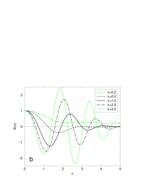
Figure 1: Scaling functions $\Phi(u)$ for Typ II as given by eq. (4.16) with $\beta_{1}+\gamma_{1}=1$ for (a) $\theta=1.5$ and (b) $\theta=2.5$, for several values of $\Lambda$ as indicated.

   

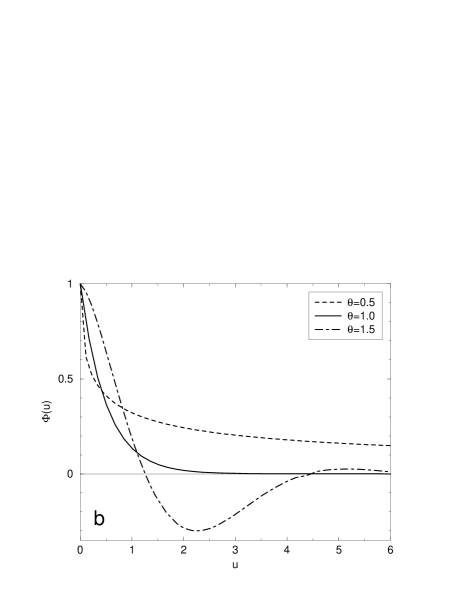
Figure 2: Scaling functions $\Phi(u)$ for Typ II as given by eq. (4.16). (a) Several values of $\theta$ as indicated, $\Lambda=1/2$ and $\beta_{1}+\gamma_{1}=1$. (b) Several values of $\theta$ and $\gamma_{1}=-\beta_{1}=1$.

In figures 1 and 2 the behaviour of the scaling function $\Phi(u)$ is illustrated for several values of $\theta$ and of $\Lambda$. The case $\beta_{1}+\gamma_{1}=1$ is governed by the properties of the function $\mathfrak{E}_{a,b}(z)$. In figure 1 for two fixed values of $\theta$ the effect of varying $\Lambda$ is displayed. Since the universal ratio $\beta_{1}/\gamma_{1}$ is arbitrary, the parameter $\Lambda$ as defined in (4.17) can take any positive value. Only for $\theta=2$ we have $\Lambda=1/2$ fixed. The dependence of the scaling function $\Phi(u)$ for $\beta_{1}+\gamma_{1}\neq 0$ on $\theta$ is shown in figure 2a, where we fix $\Lambda=1/2$. Finally, the scaling function found in the peculiar case $\beta_{1}+\gamma_{1}=0$ is illustrated in figure 2b. This case is governed by the Mittag-Leffler function $E_{\theta,1}(z)$ whose properties are reviewed in some detail in [91].

In the following cases, the asymptotic behaviour of the scaling function is algebraic, as follows from the identities, see [113]

$$E_{a,b}(-x) \simeq \frac{1}{\Gamma(b-a)}{x}^{-1}+O\left(x^{-2}\right)\;\;,\;\;0<a<2$$

$$\mathfrak{E}_{a,b}(-x) \simeq \frac{1}{b\Gamma(1-a)}x^{-1}+\frac{\Gamma(1-b)}{\Gamma(1-ab)}x^{-b}+O\left(x^{-2},x^{-1-a}\right)\;\;,\;\;1<a<3$$ (4.21)

In these cases, the physically required boundary condition is satisfied and one may deduce the relation between $\Lambda$ and the scaling dimension $x_{1}$, thereby generalizing (4.4).

We also see from figure 2 that on a qualitative level, the cases $\beta_{1}+\gamma_{1}\neq 0$ and $\beta_{1}+\gamma_{1}=0$ are broadly similar. For sufficiently small values of $\theta$, the scaling function $\Phi(u)$ descreases monotonically towards zero when $u$ increases. With increasing $\theta$, the scaling function decays faster for large $u$ and at a certain value of $\theta$ (at $\theta=2$ or $\theta=1$, respectively), the asymptotic amplitude vanishes and the decay becomes exponential. If we now increase $\theta$ slightly, the scaling function $\Phi(u)$ starts to oscillate. Oscillations also arise if for $\theta$ fixed the parameter $\Lambda$ is made sufficiently large, as can be seen from figure 1.

4.2 Scaling function for Typ I

We write eq. (3.115) in the form

$$\left(\alpha_{1}\partial_{v}^{N-1}-v^{2}\partial_{v}-v\zeta\right)\Omega(v)=0\qquad,\qquad\zeta=Nx_{1}=\frac{2x_{1}}{\theta}$$ (4.22)

It is useful to begin with the special case when $N$ is an integer [55]. Then the anisotropy exponent $\theta=2/N=2,1,\frac{2}{3},\frac{1}{2},\frac{2}{5},\frac{1}{3},\ldots$ and one merely has a finite number of generators $Y_{m}$, $m=-N/2,\ldots,N/2$. For $N=1$ and $N=2$ we recover the scaling functions found from Schrödinger and conformal invariance (see section 2) and now concentrate on the new situations $N\geq 3$.

Table 3: Some solutions $\Omega(v)$ of eq. (4.22) for $N=4$ with $\Omega(0)=1$ and their leading asymptotics for $\beta^{\prime}=0$ as $v\to\infty$. Here ${\rm I}_{\nu},{\rm K}_{\nu}$ are modified Bessel functions, ${\bf L}_{\nu}$ is a modified Struve function, ${\rm erf\,}$ is the error function (see [1]) and $\beta,\beta^{\prime}$ are constants. The abbreviation $y:=v^{2}/(2\sqrt{\alpha_{1}})$ is used throughout.

			asymptotics
$\zeta$	$\Omega(v)$		(for $\beta^{\prime}=0$)
$1$	$\left[\frac{\Gamma(3/4)^{2}}{\pi^{2}}\sqrt{y}\,{\rm K}_{1/4}^{2}\left(\frac{y}{2}\right)+\beta v{\rm I}_{1/4}\left(\frac{y}{2}\right){\rm K}_{1/4}\left(\frac{y}{2}\right)\right]$	$+\beta^{\prime}v{\rm I}_{1/4}^{2}\left(\frac{y}{2}\right)$	$4\sqrt{\alpha_{1}}\,\beta\,v^{-1}$
$2$	$\left[-\beta\sqrt{\pi}\Gamma\left(\frac{1}{4}\right)\left(\frac{y}{2}\right)^{1/4}\left[{\bf L}_{-1/4}\left(y\right)-{\rm I}_{1/4}\left(y\right)\right]\right.$		$4\sqrt{\alpha_{1}}\,\beta\,v^{-2}$
	$\left.+\Gamma\left(\frac{3}{4}\right)\left(\frac{y}{2}\right)^{1/4}\left[{\rm I}_{-1/4}\left(y\right)-{\rm I}_{1/4}\left(y\right)\right]\right]$	$+\beta^{\prime}{v}^{1/2}{\rm I}_{1/4}\left(y\right)$
$3$	$\left[e^{-y}+\beta\left(\frac{\pi^{2}\alpha_{1}}{64}\right)^{1/4}\left[e^{y}{\rm erf\,}\left(\sqrt{y}\right)-{\rm i}e^{-y}{\rm erf\,}\left({\rm i}\sqrt{y}\right)-2\sinh y\right]\right]$	$+\beta^{\prime}\,\sinh y$	$\alpha_{1}\,\beta\,v^{-3}$
$4$	$\left[1+\sqrt{\pi}\Gamma\left(\frac{3}{4}\right)\left(\frac{y}{2}\right)^{3/4}\left[{\bf L}_{1/4}\left(y\right)-{\rm I}_{-1/4}\left(y\right)\right]\right.$		$-{2\alpha_{1}}\,v^{-4}$
	$\left.+\beta\left(\frac{y}{2}\right)^{3/4}\left[{\rm I}_{-1/4}\left(y\right)-{\rm I}_{1/4}\left(y\right)\right]\right]$	$+\beta^{\prime}{v}^{3/2}{\rm I}_{1/4}\left(y\right)$

For $N=4$, some explicit solutions for a few integer values of $\zeta$ are given in table 3. Given the boundary condition $\Omega(0)=1$, these still depend on two free parameters $\beta,\beta^{\prime}$. If $\beta^{\prime}\neq 0$, these solutions diverge exponentially fast as $v\to\infty$ but if we take $\beta^{\prime}=0$, we find $\Omega(v)\sim v^{-\zeta}$ in agreement with the required boundary condition, see table 2.

Using these examples as a guide, we now study the more general case with integer $N$ and $\zeta$ arbitrary. The general solution of eq. (3.115) for integer $N\geq 2$ is readily found

$$\Omega(v)=\sum_{p=0}^{N-2}b_{p}v^{p}{\cal F}_{p}\qquad;\qquad{\cal F}_{p}={{}_{2}F_{N-1}}\left(\frac{\zeta+p}{N},1;1+\frac{p}{N},1+\frac{p-1}{N},\ldots,\frac{p+2}{N};\frac{v^{N}}{N^{N-2}\alpha_{1}}\right)$$ (4.23)

where ${{}_{2}F_{N-1}}$ is a generalized hypergeometric function and the $b_{p}$ are free parameters. To be physically acceptable, the boundary condition (3.116) must be satisfied. The leading asymptotic behaviour of the ${\cal F}_{p}$ for $v\to\infty$ can be found from the general theorems of Wright [113] (see [40] for a brief summary) and the asymptotics of $\Omega(v)$ is given by

$$\Omega(v)\simeq\sqrt{\frac{4\pi^{2}N}{N-2}}\left(\frac{v^{1/(N-2)}}{(\alpha_{1}N)^{1/N}}\right)^{\zeta+1-N}\exp\left(\frac{N-2}{N\alpha_{1}^{1/(N-2)}}v^{N/(N-2)}\right)$$ (4.24)

$$\times \sum_{p=0}^{N-2}b_{p}\,\frac{\Gamma(p+1)}{\Gamma((p+1)/N)\Gamma((p+\zeta)/N)}\left(\frac{\alpha_{1}}{N^{2}}\right)^{p/N}\left(1+O\left(v^{-N/(N-2)}\right)\right)$$

which grows exponentially as $v\to\infty$ if $N>2$. Clearly, this leading term must vanish, which imposes the following condition on the $b_{p}$

$$\sum_{p=0}^{N-2}b_{p}\,\frac{\Gamma(p+1)}{\Gamma((p+1)/N)\Gamma((p+\zeta)/N)}\left(\frac{\alpha_{1}}{N^{2}}\right)^{p/N}=0$$ (4.25)

Remarkably, this condition is already sufficient to cancel not only the leading exponential term but in fact the entire series of exponentially growing terms. Eliminating $b_{N-2}$, the final solution for $N$ integer becomes

$$\Omega(v) = \sum_{p=0}^{N-3}b_{p}\Omega_{p}(v)$$

$$\Omega_{p}(v) = v^{p}{\cal F}_{p}-\frac{\Gamma(p+1)}{\Gamma(\frac{p+1}{N})\Gamma(\frac{p+\zeta}{N})}\frac{\Gamma(\frac{N-1}{N})\Gamma(1+\frac{\zeta-2}{N})}{\Gamma(N-1)}\left(\frac{\alpha_{1}}{N^{2}}\right)^{(p+2-N)/N}v^{N-2}\,{\cal F}_{N-2}$$ (4.26)

Up to normalization, the form of $\Omega(v)$ depends on $\zeta$ and on $N-3$ free parameters $b_{p}$, while $\alpha_{1}$ merely sets a scale. The independent solutions $\Omega_{p}$ ($p=0,1,\ldots,N-3$) satisfy the boundary conditions

$$\Omega_{p}(v)\simeq\left\{\begin{array}[]{ll}v^{p}&\;;\;\mbox{\rm$v\rightarrow 0$}\\ \Omega_{p,\infty}v^{-\zeta}&\;;\;\mbox{\rm$v\rightarrow\infty$}\end{array}\right.$$ (4.27)

where explicitly

$$\Omega_{p,\infty}=-\left(\frac{\alpha_{1}}{N^{2}}\right)^{(\zeta+p)/N}\frac{\Gamma(\frac{1-\zeta}{N})}{\Gamma(1-\zeta)}\frac{\Gamma(p+1)}{\Gamma(\frac{p+1}{N})}\frac{\pi\sin\left(\frac{\pi}{N}(p+2)\right)}{\Gamma(\frac{p+\zeta}{N})\sin\left(\frac{\pi}{N}(p+\zeta)\right)\sin\left(\frac{\pi}{N}(\zeta-2)\right)}$$ (4.28)

Therefore, we have not only eliminated the entire exponentially growing series, but furthermore, the $\Omega_{p}$ satisfy exactly the physically required boundary condition (see table 2) for $v\to\infty$ [55]. Indeed, for $N=3$ this cancellation of the exponential terms is a known property of the Kummer function ${}_{1}F_{1}$ and we have for $N=3$ the scaling function

$$\Omega_{N=3}(v) = b_{0}\left[{}_{1}F_{1}\left(\frac{\zeta}{3},\frac{2}{3};\frac{v^{3}}{3\alpha_{1}}\right)-\frac{\Gamma((\zeta+1)/3)\Gamma(2/3)}{\Gamma(\zeta/3)\Gamma(4/3)}\frac{v}{(3\alpha_{1})^{1/3}}{}_{1}F_{1}\left(\frac{\zeta}{3},\frac{4}{3};\frac{v^{3}}{3\alpha_{1}}\right)\right]$$ (4.29)

$$= b_{0}\frac{\sqrt{3}}{2\pi}\Gamma\left(\frac{\zeta+1}{3}\right)\Gamma\left(\frac{2}{3}\right)U\left(\frac{\zeta}{3},\frac{2}{3};\frac{v^{3}}{3\alpha_{1}}\right)$$

where $U$ is the Tricomi function and its known asymptotic behaviour $U(a,b;z)\simeq z^{-a}$ as $z\to\infty$ [1, eq. (13.1.8)] reproduces the boundary condition eq. (4.27). We have not found an analogous statement for $N\geq 4$ in the literature. Wright’s formulas [113] simply list the dominant and the subdominant parts of the $v\to\infty$ asymptotic expansion but without any statement when the dominant part may cancel. Rather than giving a formal and lenghty proof of the cancellation of the entire asymptotic exponential series, we merely argue in favour of its plausibility through a few tests. In table 3 we list a few closed solutions for $N=4$ with satisfy the boundary condition $\Omega(0)=1$. By varying the parameters $\beta$ and $\beta^{\prime}$ one obtains the three independent solutions of the third-order differential equation (4.22). Furthermore, from the explicit form of the solutions we see that only the contribution parametrized by $\beta^{\prime}$ diverges exponentially as $v\to\infty$. There is a second solution which decays as $v^{-\zeta}$ for $v\to\infty$ and the third solution vanishes exponentially fast in the $v\to\infty$ limit. From the last two solutions we can therefore construct scaling functions with the physically expected asymptotic behaviour. In addition we illustrate the convergence of $v^{\zeta}\Omega_{p}(v)$ towards $\Omega_{p,\infty}$, as given in (4.28), by plotting $v^{\zeta}\Omega_{p}(v)$ as a function of $v$ for several values of $\zeta$.

Figure 3: Scaling functions $v^{\zeta}\Omega_{p}(v)$ for Typ I, $N=4$, $\alpha_{1}=1$ and $p=0,1$. The different curves belong to values of $\zeta=Nx_{1}$ as indicated and the squares are the values of $\Omega_{p,\infty}$.

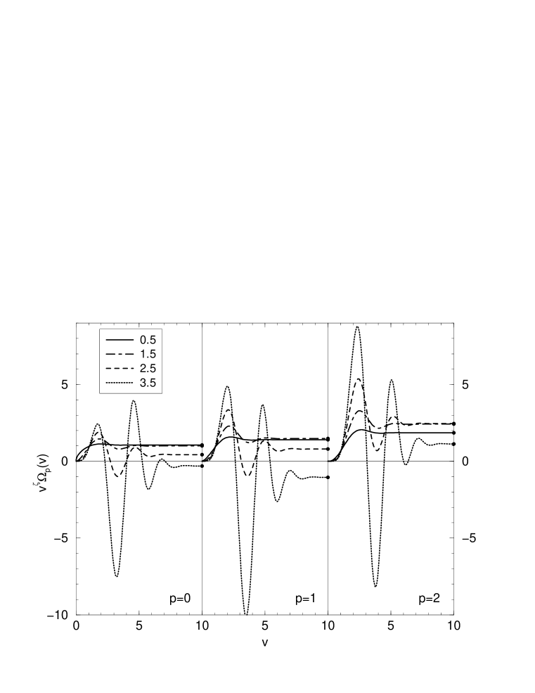
Figure 4: Scaling functions $v^{\zeta}\Omega_{p}(v)$ for Typ I, $N=5$, $\alpha_{1}=1$ and $p=0,1,2$, for different values of $\zeta=Nx_{1}$. The circles indicate the values of $\Omega_{p,\infty}$.

This is done for $N=4$ in figure 3 and for $N=5$ in figure 4 (we have also checked this for $N=6$). Besides confirming the correctness of the asymptotic expressions (4.27,4.28) for $v\to\infty$, we also see that for a large range of values of $\zeta$, the asymptotic regime is reached quite rapidly.

Below, we shall need the explicit expressions for $\Omega_{0,1}(v)$ for $N=4$

$$\Omega_{0}(v) = \frac{\Gamma(3/4)}{\Gamma(\zeta/4)}\sum_{n=0}^{\infty}\frac{\Gamma(n/2+\zeta/4)}{n!\Gamma(n/2+3/4)}\left(-\frac{v^{2}}{2\sqrt{\alpha_{1}}}\right)^{n}$$ (4.30)

$$\Omega_{1}(v) = \sqrt{\frac{\pi}{2}}\frac{v}{\Gamma((\zeta+1)/4)}\sum_{n=0}^{\infty}\frac{\Gamma((n+1+\zeta)/4)s(n)}{\Gamma(n/4+1)\Gamma((n+3)/2)}\left(-\frac{v}{\sqrt[4]{4\alpha_{1}}}\right)^{n}$$

where $s(n):=\frac{1}{\sqrt{2}}\left(\cos\frac{n\pi}{4}+\sin\frac{n\pi}{4}\right)\cos\frac{n\pi}{4}$. These expressions will be encountered again in section 5 for the correlators of the ANNNI and ANNNS models at their Lifshitz points.

Next, we study what happens for $N$ not an integer. It is useful to write the anisotropy exponent as

$$\frac{2}{\theta}=N=N_{0}+\varepsilon\;\;,\;\;\varepsilon=\frac{p}{q}$$ (4.31)

where $N_{0}\in\mathbb{N}$ and $p,q$ are positive coprime integers.

For $N$ integer, we have seen that there is an unique solution which decays as $\Omega(v)\sim v^{-\zeta}$ as $v\to\infty$. The presence of such a solution for arbitrary $N$ may be checked by seeking solutions of the form

$$\Omega(v)=\sum_{n=0}^{\infty}a_{n}v^{-n/q+s}\;\;,\;\;a_{0}\neq 0$$ (4.32)

In making this ansatz, we concentrate on those solutions of eq. (4.22) which do not grow or vanish exponentially for $v$ large. As done before for Typ II, and under the same conditions, we find upon substitution

$$\sum_{n=p+qN_{0}}^{\infty}\frac{\alpha_{1}\Gamma\left(\frac{1}{q}(-n+p+qN_{0})+s+1\right)}{\Gamma\left(-\frac{n}{q}+2+s\right)}a_{n-p-qN_{0}}v^{-n/q}+\sum_{n=0}^{\infty}\left(\frac{1}{q}(n-px_{1}-qN_{0}x_{1})-s\right)a_{n}v^{-n/q}=0$$ (4.33)

which must be valid for all positive values of $v$. Comparing the coefficients of $v$, we obtain

$$s = -\frac{p}{q}x_{1}-N_{0}x_{1}=-(N_{0}+\varepsilon)x_{1}=-\zeta$$

$$a_{n} = 0\quad;\quad\mbox{\rm for~{}~{}}n=1,2,\ldots,p+qN_{0}-1$$ (4.34)

$$\frac{n}{q}a_{n} = -\frac{\alpha_{1}\Gamma\left(-\frac{1}{q}(n-p(1+x_{1})-qN_{0}(1+x_{1}))+1\right)}{\Gamma\left(-\frac{n}{q}-\frac{p}{q}x_{1}-N_{0}x_{1}+2\right)}\,a_{n-p-qN_{0}}$$

In principle, there might be additional $\delta$-function terms which come from the definition (A2) of the fractional derivative, see appendix A. However, if we either restrict to $v>0$ or else if $\zeta$ is distinct from the discrete set of values $\zeta_{c}=2+m-n/q$, where $n,m\in\mathbb{N}$, these terms do not occur.

We can now let $n=(p+qN_{0})\ell$ and $a_{n}=a_{(p+qN_{0})\ell}=:b_{\ell}$ and find the simpler recurrence

$$b_{\ell}=-\frac{\alpha_{1}}{N\ell}\frac{\Gamma(1+N-(\ell+x_{1})N)}{\Gamma(2-(\ell+x_{1})N)}\,b_{\ell-1}\;\;,\;\;\ell=1,2,\ldots$$ (4.35)

which can be solved in a manner analogous to the one used for Typ II before, with the result

$$b_{\ell}=b_{0}\left(\frac{\alpha_{1}}{N^{2}}\right)^{\ell}\frac{\Gamma\left(1+(\zeta-1)/N\right)}{\ell!\,\Gamma\left(\ell+1+(\zeta-1)/N\right)}\frac{\Gamma(1-\zeta)}{\Gamma(1-\zeta-\ell N)}$$ (4.36)

In the special case $N=1$, the resulting series may be summed straightforwardly and leads to the elementary result $\Omega_{N=1}(v)=b_{0}v^{-\zeta}e^{-\alpha_{1}/v}$, where $v=tr^{-2}$ and $\zeta=x_{1}$. We thus recover the form (2.24) of Schrödinger invariance for the two-point function $\langle\phi\phi^{*}\rangle$, as it should be.

If we use the identity $\Gamma(x)\Gamma(1-x)=\pi/\sin(\pi x)$ and define the function

$$\mathfrak{G}_{a,b}^{(N)}(z):=\Gamma(b)\Gamma(1-a)\sum_{\ell}^{\infty}\frac{\Gamma(\ell N+a)}{\ell!\,\Gamma(\ell+b)}\,z^{\ell}$$ (4.37)

the series solution with the requested behaviour $\Omega(v)\simeq b_{0}v^{-\zeta}$ at $v\to\infty$ may be written as follows

$$\Omega(v) = v^{-\zeta}\sum_{\ell=0}^{\infty}b_{\ell}\,v^{-N\ell}$$

$$= b_{0}v^{-\zeta}\sum_{\ell=0}^{\infty}\frac{\Gamma\left(1+(\zeta-1)/N\right)}{\Gamma(\zeta)}\frac{\sin\left(\pi(N\ell+\zeta)\right)}{\sin\pi\zeta}\frac{\Gamma(\ell N+\zeta)}{\ell!\,\Gamma\left(l+1+(\zeta-1)/N\right)}\left(\frac{\alpha_{1}}{N^{2}}\frac{1}{v^{N}}\right)^{\ell}~{}~{}~{}~{}~{}$$

$$= \frac{b_{0}}{2\pi{\rm i}}v^{-\zeta}\left[e^{\pi{\rm i}\zeta}\mathfrak{G}_{\zeta,1+\frac{\zeta-1}{N}}^{(N)}\left(\frac{\alpha_{1}}{N^{2}}e^{\pi{\rm i}N}v^{-N}\right)-e^{-\pi{\rm i}\zeta}\mathfrak{G}_{\zeta,1+\frac{\zeta-1}{N}}^{(N)}\left(\frac{\alpha_{1}}{N^{2}}e^{-\pi{\rm i}N}v^{-N}\right)\right]$$

From these expressions, it is clear that the radius of convergence of these series as a function of the variable $1/v$ is infinite for $N<2$ and zero for $N>2$. In the first case, we therefore have a convergent series for the scaling function, while in the second case, we have obtained an asymptotic expansion.

In several applications, notably the $3D$ ANNNI model to be discussed in the next section, the anisotropy exponent $\theta\simeq 1/2$ to a very good approximation. Therefore, consider fractional derivatives of order $a=N_{0}+\varepsilon$, where $N_{0}$ is an integer and $\varepsilon$ is small. To study perturbatively the solutions for $\varepsilon\ll 1$, we use the identity (A12), set $a=N=N_{0}+\varepsilon$ and expand to first order in $\varepsilon$. The result is

$$\left.\partial_{r}^{N}f(r)\right|_{\rm reg} = \partial_{r}^{\varepsilon}\partial_{r}^{N_{0}}f(r)$$ (4.39)

$$\simeq f^{(N_{0})}(r)+\varepsilon{\cal L}_{0}f^{(N_{0})}(r)+O\left(\varepsilon^{2}\right)$$

$${\cal L}_{0}g(r) = \left[-\left(C_{E}+\ln r\right)+\sum_{\ell=1}^{\infty}\frac{(-1)^{\ell+1}}{\ell!\,\ell}\,r^{\ell}\frac{{\rm d}^{\ell}}{{\rm d}r^{\ell}}\right]g(r)$$

where $C_{E}=0.5772\ldots$ is Euler’s constant. To find the first correction in $\varepsilon$ with respect to the solution (4.26) when $N$ is an integer, we set again $N=N_{0}+\varepsilon$ with $N_{0}\in\mathbb{N}$ and $\varepsilon>0$ and consider

$$\Omega(v)=\Omega^{(0)}(v)+\varepsilon\Omega^{(1)}(v)+O\left(\varepsilon^{2}\right)$$ (4.40)

Then $\Omega^{(0)}(v)$ solves eq. (4.22) with $N=N_{0}$ and is consequently given by eq. (4.26), whereas $\Omega^{(1)}(v)$ satisfies the equation

$$\left(\alpha_{1}\partial_{v}^{N_{0}-1}-v^{2}\partial_{v}-\zeta v\right)\Omega^{(1)}(v)=\omega(v):=-{\cal L}_{0}\left(v^{2}\partial_{v}+\zeta v\right)\Omega^{(0)}(v)$$ (4.41)

which we now study.

First, we consider the limiting behaviour of $\Omega^{(1)}(v)$ for $v$ either very large or very small. If $v\gg 1$, we see from eq. (4.2) that $\Omega^{(0)}(v)\sim v^{-\zeta}(1+{\rm O}(v^{-N_{0}}))$. This implies in turn that $\omega(v)\simeq(A_{\infty}+B_{\infty}\ln v)v^{-\zeta-(N_{0}-1)}$, where $A_{\infty},B_{\infty}$ are some constants. Therefore one must have $\Omega^{(1)}(v)\sim v^{-\zeta}(1+{\rm O}(v^{-N_{0}}))$ in order to reproduce this result for $\omega(v)$. On the other hand, if $v\ll 1$, we have $\Omega^{(0)}(v)\simeq{\rm cste.}$ which leads to $\omega(v)\simeq(A_{0}+B_{0}\ln v)$ with some constants $A_{0},B_{0}$. This can be reproduced from the limiting behaviour $\Omega^{(1)}(v)\sim{\rm O}(v,v^{N_{0}}\ln v)$. In conclusion, the first-order perturbation is compatible with the boundary condition (3.116) for the full scaling function $\Omega(v)$.

We now work out the first correction $\Omega^{(1)}(v)$ explicitly for $N_{0}=4$. This is the case we shall need in section 5. There are two physically acceptable solutions $\Omega_{0}^{(0)}(v)$ and $\Omega_{1}^{(0)}(v)$ of zeroth order in $\varepsilon$ which are given in (4.30). The general zeroth-order solution is given by

$$\Omega^{(0)}(v)=\Omega_{0}^{(0)}(v)+\frac{\mathfrak{p}}{\alpha_{1}^{1/4}}\Omega_{1}^{(0)}(v)$$ (4.42)

where $\mathfrak{p}=b_{1}\alpha_{1}^{1/4}/b_{0}$ is a universal constant. Then all metric factors in the scaling function are absorbed into the argument $v/\alpha_{1}^{1/4}$ and the form of $\Omega(v)$ is given by the two universal parameters $\zeta$ and $\mathfrak{p}$.

Consider the first-order correction to $\Omega^{(0)}(v)$. From the explicit form of ${\cal L}_{0}$ and (4.30), we have

$$\omega(v)=\sum_{n=0}^{\infty}\left[A_{n}v^{n+1}+B_{n}v^{n+1}\ln v\right]$$ (4.43)

where $A_{n}=-\psi(n+1)B_{n}$ and

$$B_{n}=\left\{\begin{array}[]{ll}\frac{\Gamma(n+\zeta/4)\,\Gamma(3/4)}{\Gamma(n+3/4)\,\Gamma(\zeta/4)}\frac{4n+\zeta}{(2n)!}\left(\frac{1}{4\alpha_{1}}\right)^{n}&;~{}~{}n\equiv 0\bmod 4\\ \frac{1}{\alpha_{1}^{1/4}}\frac{\sqrt{\pi}\,\Gamma(n+(\zeta+1)/4)}{\Gamma((\zeta+1)/4)\,\Gamma(2n+3/2)}\frac{4n+1+\zeta}{n!\>2}\left(\frac{1}{4\alpha_{1}}\right)^{n}\mathfrak{p}&;~{}~{}n\equiv 1\bmod 4\\ -\frac{1}{\sqrt{\alpha_{1}}}\frac{\Gamma(n+(\zeta+2)/4)}{2\,\Gamma(n+5/4)}\frac{4n+2+\zeta}{(2n+1)!}\left(\frac{1}{4\alpha_{1}}\right)^{n}\left[\frac{\Gamma(3/4)}{\Gamma(\zeta/4)}+\mathfrak{p}\frac{1}{\Gamma((\zeta+1)/4)}\sqrt{\frac{\pi}{2}}\right]&;~{}~{}n\equiv 2\bmod 4\\ 0&;~{}~{}n\equiv 3\bmod 4\end{array}\right.$$ (4.44)

Here $\psi(z)=\Gamma^{\prime}(z)/\Gamma(z)$ is the digamma function [1] and the identity

$$\sum_{\ell=1}^{\infty}\left(\mbox{${\begin{array}[]{c}\alpha\\ \ell\end{array}}$}\right)\frac{(-1)^{\ell+1}}{\ell}=C_{E}+\psi(\alpha+1)$$ (4.45)

was used. The solution of the third-order differential equation (4.41) is of the form

$$\Omega^{(1)}(v)=\sum_{n=0}^{\infty}\left[a_{n}v^{n}+b_{n}v^{n}\ln v\right]$$ (4.46)

where in addition

$$a_{0}=a_{3}=0\;\;,\;\;b_{0}=b_{1}=b_{2}=b_{3}=0$$ (4.47)

and, for all $n\geq 0$

$$b_{n+4} = \frac{1}{\alpha_{1}\,(n+4)(n+3)(n+2)}\left[B_{n}+b_{n}\left(n+\zeta\right)\right]$$

$$a_{n+4} = \frac{1}{\alpha_{1}\,(n+4)(n+3)(n+2)}\left[A_{n}+a_{n}\left(n+\zeta\right)+b_{n}-b_{n+4}\alpha_{1}\left(3n^{2}+18n+26\right)\right]$$ (4.48)

The value of the constant $a_{0}$ is fixed because of the boundary condition $\Omega(0)=1$. The first perturbative correction $\Omega^{(1)}(v)$ still depends on the free parameters $a_{1}=:\mathfrak{p}\,\mathfrak{a}$ and $a_{2}=:\mathfrak{b}$. We also observe that because of (4.44), we have $a_{4n+3}=b_{4n+3}=0$ for all $n\in\mathbb{N}$ and that the metric factor $\alpha_{1}$ merely sets the scale in the variable $v/\alpha_{1}^{1/4}$ but does not otherwise affect the functional form of $\Omega^{(1)}(v)$.

We have seen above that for $v\gg 1$, we must recover $\Omega(v)\sim v^{-\zeta}$. We can therefore fix $\mathfrak{a}$ and $\mathfrak{b}$ such that the correction term $\Omega^{(1)}(v)$ goes to zero for $v$ large. Furthermore, we see from figure 3 that the asymptotic regime is already reached for quite small values of $v$ for a large range of values of $\zeta$. To a good approximation, we can therefore determine $\mathfrak{a}$ and $\mathfrak{b}$ from the requirement that $\Omega^{(1)}(v_{0})=0$ and ${\rm d}\Omega^{(1)}(v_{0})/{\rm d}v=0$ if $v_{0}$ is finite, but chosen to be sufficiently large. The recursion (4.48) then gives a system of two linear equations for $\mathfrak{a}$ and $\mathfrak{b}$.

   

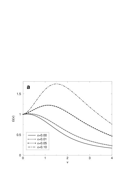
Figure 5: Perturbative scaling functions $\Omega(v)$ eq. (4.40) for Typ I around $N_{0}=4$, with $\zeta=1.3$, $\alpha_{1}=1$ and (a) $\mathfrak{p}=+0.11$ and (b) $\mathfrak{p}=-0.11$, for several values of $\varepsilon$.

As an example, we illustrate this in figure 5 for $\zeta=1.3$. From figure 3, we observe that $v_{0}=6$ is already far in the asymptotic regime. For the values $\mathfrak{p}=\pm 0.11$, the scaling function (4.40), with the first-order correction included, is shown for several values of $\varepsilon=N-4$. The first-order perturbative corrections with respect to the solution found for $N=4$ are quite substantial, even for small values of $\varepsilon$. This suggests that a non-integer value of $N$ in the differential equation (4.22) should be readily detectable in numerical simulations. We shall come back to this in section 5 in the context of the $3D$ ANNNI model.

The full series solution leads to difficulties with the boundary condition $\Omega(0)=1$. This is further discussed in appendix D.

5 Applications

5.1 Uniaxial Lifshitz points

Uniaxial Lifshitz points [64] are paradigmatic examples of equilibrium spin systems with a strongly anisotropic critical behaviour. They are conveniently realized in spin systems with competing interactions. Besides the well-known uniaxially modulated magnets, alloys and ferroelectrics [114, 106, 81], recently found new examples include ferroelectric liquid crystals, uniaxial ferroelectrics, block copolymers, spin-Peierls and quantum systems [109, 111, 7, 85, 104]. For the sake of notational simplicity, we merely consider uniaxial competing interactions, which are described by the Hamiltonian

$${\cal H}=-J\sum_{(\boldsymbol{i},\boldsymbol{j})}s_{\boldsymbol{i}}s_{\boldsymbol{j}}+\kappa_{1}J\sum_{\boldsymbol{i}}s_{\boldsymbol{i}}s_{\boldsymbol{i}+2\boldsymbol{e}_{\|}}+\kappa_{2}J\sum_{\boldsymbol{i}}s_{\boldsymbol{i}}s_{\boldsymbol{i}+3\boldsymbol{e}_{\|}}$$ (5.1)

where $s_{\boldsymbol{i}}$ are the spin variables at site $\boldsymbol{i}$. We shall consider here the ANNNI model, where $s_{\boldsymbol{i}}=\pm 1$ are Ising spins and the ANNNS model, where the $s_{\boldsymbol{i}}\in\mathbb{R}$ and satisfy the spherical constraint $\sum_{\boldsymbol{i}}s_{\boldsymbol{i}}^{2}={\cal N}$, where $\cal N$ is the total number of sites of the lattice. The first sum runs only over pairs of nearest-neighbour sites of a hypercubic lattice in $d=d_{\perp}+1$ dimensions. In the second and third sums, additional interactions between second and third neighbours are added along a chosen axis ($\|$) and $\boldsymbol{e}_{\|}$ is the unit vector in this direction. Finally, $J>0$ and $\kappa_{1,2}$ are coupling constants. For reviews, see [114, 106, 107, 81, 33].

In order to understand the physics of the model, we take $\kappa_{2}=0$ for a moment. If in addition $\kappa_{1}$ is small, the model undergoes at some $T_{c}=T_{c}(\kappa_{1})$ a second-order phase transition which is in the Ising or spherical model universality class, respectively, for the systems considered here. However, if $\kappa_{1}$ is large and positive, the zero-temperature ground state may become spatially modulated and a rich phase diagram is obtained [114, 106, 107, 81]. A particular multicritical point is the meeting point of the disordered paramagnetic, the ordered ferromagnetic and the ordered incommensurate phase. This point is called an uniaxial Lifshitz point (of first order) [64]. If one now lets vary $\kappa_{2}$, one obtains a line of Lifshitz points of first order. This line terminates in a Lifshitz point of second order [83, 105]. Lifshitz points of order $L-1$ can be defined analogously and exist at non-zero temperatures for $d>d_{*}$ [105]. For the ANNNS model, the lower critical dimension is

$$d_{*}:=2+(L-1)/L$$ (5.2)

Close to a Lifshitz point, the scaling of the correlation functions $C(r_{\|},\boldsymbol{r}_{\perp})$ is strongly direction-dependent. Here $r_{\|}$ is the distance along the chosen axis with the competing interactions and $\boldsymbol{r}_{\perp}$ is the distance vector in the remaining $d_{\perp}$ directions where only nearest-neighbour interactions exist. Slightly off criticality, correlations decay exponentially, but the scaling of the correlation lengths is direction-dependent

$$\xi_{\|}\sim\left(T-T_{L}\right)^{-\nu_{\|}}\;\;,\;\;\xi_{\perp}\sim\left(T-T_{L}\right)^{-\nu_{\perp}}$$ (5.3)

where $T_{L}$ is the location of the Lifshitz point. The anisotropy between the axial ($\|$) and the other ($\perp$) directions is measured in terms of the anisotropy exponent

$$\theta=\nu_{\|}/\nu_{\perp}$$ (5.4)

Precisely at the Lifshitz point, one expects

$$C_{\sigma}(r_{\|},\boldsymbol{0})\sim r_{\|}^{-2x_{\sigma}/\theta}\;\;,\;\;C_{\sigma}(0,\boldsymbol{r}_{\perp})\sim r_{\perp}^{-2x_{\sigma}}\;\;,\;\;C_{\varepsilon}(r_{\|},\boldsymbol{0})\sim r_{\|}^{-2x_{\varepsilon}/\theta}\;\;,\;\;C_{\varepsilon}(0,\boldsymbol{r}_{\perp})\sim r_{\perp}^{-2x_{\varepsilon}}$$ (5.5)

for the connected spin-spin correlator $C_{\sigma}$ and the connected energy-energy correlator $C_{\varepsilon}$, respectively, and where $x_{\sigma}$ and $x_{\varepsilon}$ are scaling dimensions. The critical exponents $\alpha,\beta,\gamma$ are defined as usual from the specific heat, the order parameter and the susceptibility, but some of the familiar scaling relations valid for isotropic systems (where $\theta=1$) must be replaced by

$$2-\alpha=d_{\perp}\nu_{\perp}+\theta\nu_{\|}\;\;,\;\;\gamma=\left(2-\eta_{\perp}\right)\nu_{\perp}=\left(2/\theta-\eta_{\|}\right)\nu_{\|}$$ (5.6)

where the anomalous dimensions $\eta_{\|,\perp}$ are defined from the spin-spin correlator

$$C_{\sigma}(0,\boldsymbol{r}_{\perp})\sim r_{\perp}^{-[d_{\perp}+\theta-2+\eta_{\perp}]}\;\;,\;\;C_{\sigma}(r_{\|},\boldsymbol{0})\sim r_{\|}^{-[(d_{\perp}+\theta-2)/\theta+\eta_{\|}]}$$ (5.7)

and are related via $\eta_{\|}=\eta_{\perp}/\theta$. Alternatively, one often works with exponents $\nu_{\ell 2}=\nu_{\perp}$, $\nu_{\ell 4}=\nu_{\|}$, $\eta_{\ell 2}=\eta_{\perp}$ and $\eta_{\ell 4}=\eta_{\|}+4-2/\theta$, see e.g. [64, 30]. Then $\gamma=(4-\eta_{\ell 4})\nu_{\ell 4}=(2-\eta_{\ell 2})\nu_{\ell 2}$.

Standard renormalization group arguments lead to the following anisotropic scaling of the correlation functions

$$C_{\sigma,\varepsilon}(r_{\|},\boldsymbol{r}_{\perp})=b^{-2x_{\sigma,\varepsilon}}C_{\sigma,\varepsilon}(r_{\|}b^{-\theta},\boldsymbol{r}_{\perp}b^{-1})=r_{\perp}^{-\zeta_{\sigma,\varepsilon}\theta}\Omega_{\sigma,\varepsilon}\left(r_{\|}/r_{\perp}^{\theta}\right)$$ (5.8)

for both the spin-spin and the energy-energy correlators, respectively. For a Lifshitz point in $(d_{\perp}+1)$ dimensions, we have

$$\zeta_{\sigma}=\frac{2(\theta+d_{\perp})}{\theta(2+\gamma/\beta)}\;\;,\;\;\zeta_{\varepsilon}=\frac{2(\theta+d_{\perp})(1-\alpha)}{\theta(2-\alpha)}$$ (5.9)

We want to compare the form of the spin-spin correlator with the predictions of local scale invariance. We begin with Lifshitz points of first order. Then, as will be discussed further below, $\theta\simeq\frac{1}{2}$ at least to a good approximation. In terms of the notation of sections 3 and 4, this corresponds to $N=2/\theta=4$. For $N=4$, we recall the two-point function of Typ I

$$C(r_{\|},\boldsymbol{r}_{\perp})=r_{\perp}^{-\zeta/2}\>b_{0}\>\left(\Omega_{0}(v)+\frac{\mathfrak{p}}{\alpha_{1}^{1/4}}\Omega_{1}(v)\right)\;\;,\;\;v=tr^{-1/2}$$ (5.10)

where $\Omega_{0,1}(v)$ are explicitly given in eq. (4.30). The functional form of $\Omega(v)$ only depends on the universal parameters $\zeta$ and $\mathfrak{p}$. The metric factor $\alpha_{1}$ only arises as a scale factor through the argument $v\,\alpha_{1}^{-1/4}$.

We shall now present tests of the two-point function of Typ I of local scale invariance in three distinct universality classes.

1. Our first example is the exactly solvable ANNNS model. The phase diagram is well-known and uniaxial Lifshitz points of first order occur along the line [83, 105, 40]

$$\kappa_{2}=\frac{1}{9}\left(1-4\kappa_{1}\right)\;\;,\;\;\kappa_{1}<\frac{2}{5}$$ (5.11)

with a known $T_{L}=T_{L}(\kappa_{1},\kappa_{2})$. The lower critical dimension $d_{*}=\frac{5}{2}$. We need the following exactly known critical exponents in $d$ dimensions [83, 105]

$$\beta=\frac{1}{2}\;\;,\;\;\gamma=\frac{4}{2d-5}\;\;,\;\;\theta=\frac{1}{2}\;\;,\;\;\zeta_{\sigma}=2\left(d-\frac{5}{2}\right)$$ (5.12)

which means $N=4$ in our notation. The exact spin-spin correlator along the line (5.11) of Lifshitz points is [40]

$$C_{\sigma}(r_{\|},\boldsymbol{r}_{\perp}) = C_{0}\>r_{\perp}^{-(d-d_{*})}\Psi\left(\frac{d-d_{*}}{2},\frac{1}{4}\sqrt{\frac{3}{2-5\kappa_{1}}}\frac{r_{\|}^{2}}{r_{\perp}}\right)$$ (5.13)

$$\Psi(a,x) = \sum_{k=0}^{\infty}\frac{(-1)^{k}}{k!}\frac{\Gamma(k/2+a)}{\Gamma(k/2+3/4)}x^{k}$$ (5.14)

where $C_{0}$ is a (known) normalization constant. This reproduces the exponent $\zeta_{\sigma}$ from eq. (5.12). Comparing with the expected form (5.10) and the specific functions (4.30), we see that

$$\Omega_{0}(v)=\frac{\Gamma(3/4)}{\Gamma(\zeta_{\sigma}/4)}\Psi\left(\frac{\zeta_{\sigma}}{4},\frac{v^{2}}{2\sqrt{\alpha_{1}}}\right)$$ (5.15)

With the correspondence $t\leftrightarrow r_{\|}$, $r\leftrightarrow r_{\perp}$ and the non-universal metric factor $\alpha_{1}=\frac{4}{3}(2-5\kappa_{1})$, we therefore observe complete agreement. In particular, we identify the universal parameter $\mathfrak{p}=0$ [55].

2. Next, we consider the uniaxial Lifshitz point in the $3D$ ANNNI model. Two complimentary approaches have been used. First, the model may be formulated in terms of a $n$-component field $\boldsymbol{\phi}(r_{\|},\boldsymbol{r}_{\perp})$ with a global O($n$)-symmetry and spatially anisotropic interactions [64]. This model, which might be called ANNNO($n$) model, reduces to the ANNNI model in the special case $n=1$ and gives the ANNNS model in the $n\to\infty$ limit. Recently, Diehl and Shpot [30, 108, 31, 32, 33] studied very thoroughly the field-theoretic renormalization group of the ANNNO($n$) model at the Lifshitz point at the two-loop level and derived the critical exponents to second order in the $\varepsilon$-expansion, where $\varepsilon=4.5-d$. Second, one may resort to numerical methods, such as series expansions [86, 80] or Monte Carlo simulations. While older simulational studies [68] were restricted to small systems, the use of modern cluster algorithms [112] allows to simulate considerably larger systems. The Wolff algorithm can be adapted to systems with competing interactions beyond nearest neighbours such as the ANNNI model [90, 59]. In addition, a recently proposed scheme [36] permits the direct computation of two-point functions on an effectively infinite lattice. That technique can be extended to ANNNI models as well [90, 59].

Table 4: Estimates for the location of the uniaxial Lifshitz point of the $3D$ ANNNI model on a cubic lattice. The numbers in brackets give the uncertainty in the last digit(s).

$T_{L}$	$\kappa_{1,L}$
3.73(3)	0.270(5)	high-temperature series	[86]
3.77(2)	0.265	Monte Carlo	[68]
3.7475(50)	0.270(4)	cluster Monte Carlo	[90]

Before the scaling form of any correlator can be tested, the Lifshitz point must be located precisely. In table 4 we show some estimates for the coupling $\kappa_{1,L}$ and the Lifshitz point critical temperature $T_{L}$. Here the ANNNI Hamiltonian (5.1) with $\kappa_{2}=0$ on a $3D$ simple cubic lattice was used. The increase in precision coming from the new cluster algorithm is evident and we take the estimates obtained in [90] as the location of the Lifshitz point.

Table 5: Estimates for critical exponents at the uniaxial Lifshitz point of the $3D$ ANNNI model. The numbers in brackets give the uncertainty in the last digit(s).

$\alpha$	$\beta$	$\gamma$	$\theta$
0.20(15)		1.62(12)		high-temperature series	[80]
	0.19(2)	1.40(6)		Monte Carlo	[68]
0.160	0.220	1.399	0.487	renormalized field theory	[108, 33]
0.18(2)	0.238(5)	1.36(3)		cluster Monte Carlo	[90]

Next, the anisotropy exponent $\theta$ and the scaling dimension $\zeta_{\sigma}$ must be found. While it had been believed for a long time that also for the ANNNI model $\theta=\frac{1}{2}$ might hold, it has been recently established that to the second order in the $\varepsilon$-expansion $\theta=\frac{1}{2}-\mathfrak{a}\varepsilon^{2}+O(\varepsilon^{3})$, where $\mathfrak{a}\simeq 0.0054$ in the $3D$ ANNNI model [30]. In table 5 we list two older and the most recent estimates for the Lifshitz point critical exponents $\alpha,\beta,\gamma$ and $\theta$. A direct determination of $\theta$ from simulational data is not yet possible. Since in [90] the exponents $\alpha,\beta,\gamma$ were determined independently, their agreement with the scaling relation $\alpha+2\beta+\gamma=2$ to within $\approx 0.8\%$ allows for an a posteriori check on the quality of the data. For details on the simulational methods we refer to [90, 59].

If we take the exponent estimates of [90] and in addition set $\theta=\frac{1}{2}$, we find from (5.9) for the $3D$ ANNNI model ($d_{\perp}=2$)

$$\zeta_{\sigma}=1.30\pm 0.05\;\;,\;\;\zeta_{\varepsilon}=4.5\pm 0.2$$ (5.16)

where the errors follow from the quoted uncertainties in the determination of the exponents $\alpha,\beta,\gamma$. If we now take $\theta=0.48$ as suggested by two-loop results of [108], the resulting variation of both $\zeta_{\sigma}$ and $\zeta_{\varepsilon}$ stays within the error bars quoted in eq. (5.16). In conclusion, given the precision of the available exponent estimates, any effects of a possible deviation of $\theta$ from $\frac{1}{2}$ are not yet notable. We shall therefore undertake the subsequent analysis of the correlator by making the working hypothesis $\theta=\frac{1}{2}$ [90].

 

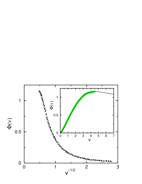
Figure 6: Scaling function $\Phi(u)$ as defined in (5.17) for the $3D$ ANNNI model, for $\kappa_{1}=0.270$ and $T=3.7475$. Selected data on a $200\times 200\times 100$ lattice are shown. The symbols correspond to several values of $r_{\perp}$. The inset shows the full data set (gray points) and the prediction (5.10) of local scale invariance with $N=4$ and $\mathfrak{p}=-0.11$, $\alpha_{1}=33.2$ and $b_{0}=0.41$. The data are from [90].

In this case, we can compare with the scaling prediction (5.10) obtained for $N=2/\theta=4$. In figure 6 we show data [90] for the modified scaling function of the spin-spin correlator

$$\Phi(v)=v^{\zeta_{\sigma}}\Omega_{\sigma}(v)$$ (5.17)

The clear data collapse establishes scaling. It can be checked that there is no perceptible change in the scaling plot for values of $\theta$ slightly less than $\frac{1}{2}$ [90].

For a quantitative comparison with (5.10), one may consider the moments

$$M(n)=\int_{0}^{\infty}\!{\rm d}v\,v^{n}\Phi(v)$$ (5.18)

Then it is easy to show [9] that the moment ratios

$$J_{k}\left(\left\{m_{i}\right\};\left\{n_{j}\right\}\right)=\left.\prod_{i=1}^{k}M(m_{i})\right/\prod_{j=1}^{k}M(n_{j})\;\;,\;\;\mbox{\rm~{}~{}with~{}~{}}\sum_{i=1}^{k}m_{i}=\sum_{j=1}^{k}n_{j}$$ (5.19)

and $k\geq 2$ are independent of $b_{0}$ and $\alpha_{1}$. They only depend on the functional form of $\Phi(u)$. This in turn is determined by $\zeta_{\sigma}$ and $\mathfrak{p}$. Therefore, the determination of a certain moment ratio allows, with $\zeta_{\sigma}$ given by (5.16), to find a value for $\mathfrak{p}$. The Monte Carlo data will be consistent with (5.10) if the values of $\mathfrak{p}$ found from several distinct ratios $J_{k}$ coincide. In practise, these integrals cannot be calculated up to $v=\infty$ but only to some finite value $v_{0}$ and the moments retain a dependence on $\alpha_{1}$ through the upper limit of integration. Then an iteration procedure must be used to find $\mathfrak{p}$ and $\alpha_{1}$ simultaneously [90]. The results are collected in table 6.

Table 6: Values of the parameters $\mathfrak{p}$ and $\alpha_{1}$ as determined from different moment ratios $J_{k}\left(\left\{m_{i}\right\};\left\{n_{j}\right\}\right)$.

$k$	$\{m_{i}\}$	$\{n_{j}\}$	$\mathfrak{p}$	$\alpha_{1}$
2	$\{0,-0.5\}$	$\{-0.25,-0.25\}$	-0.102	32.7
2	$\{-0.25,-0.75\}$	$\{-0.5,-0.5\}$	-0.125	34.0
2	$\{0.2,-0.9\}$	$\{0,-0.7\}$	-0.100	32.8
3	$\{0.2,-0.6,-0.8\}$	$\{-0.3,-0.4,-0.5\}$	-0.102	32.8
3	$\{-0.1,-0.6,-0.7\}$	$\{-0.4,-0.5,-0.5\}$	-0.117	33.5

Clearly, the two parameters can be consistently determined from different moment ratios. The final estimate is [90]

$$\mathfrak{p}=-0.11\pm 0.01\;\;,\;\;\alpha_{1}=33.2\pm 0.8$$ (5.20)

Since we have seen above that $\mathfrak{p}=0$ for the spin-spin correlator of the ANNNS model, it follows that the value of $\mathfrak{p}$ is characteristic for the universality class at hand.

In figure 6 the Monte Carlo data are compared with the resulting scaling function, after fixing the overall normalization constant $b_{0}=0.41$. The agreement between the data and the prediction (5.10) of local scale invariance is remarkable.

To finish, we reconsider our working hypothesis $\theta=\frac{1}{2}$. Indeed, in figure 5 we had shown how the form of the scaling function $\Omega(v)$ changes when $\varepsilon=N-4$ is increased, to first order in $\varepsilon$. In particular, rather pronounced non-monotonic behaviour is seen for values of $\varepsilon\sim 0.1$ which is the order of magnitude suggested from the results of renormalized field theory [30, 108, 33], see table 5. Nothing of this is visible in the Monte Carlo data of figure 6. Assuming that first-order perturbation theory in $\varepsilon$ as described in section 4 is applicable here, we conclude from this observation that $\varepsilon$ should be significantly smaller. Given the differences between the exponent estimates coming from renormalized field theory [108] and cluster Monte Carlo [90], a possible difference of $\theta$ from $\frac{1}{2}$ cannot yet be unambigously detected. Direct precise estimates of $\theta$ are needed.

A similar analysis can be performed for the energy-energy correlation function. This will be described elsewhere.

In summary, having confirmed local scale invariance for the spin-spin correlator at the Lifshitz points in the ANNNI and the ANNNS models, it is plausible that the same will hold true for all ANNNO($n$) models with $1\leq n\leq\infty$.

3. Finally, we consider the Lifshitz point of second order in the ANNNS model. In the ANNNS model as defined in eq. (5.1), a second-order Lifshitz point occurs at the endpoint

$$\kappa_{1}=\frac{2}{5}\;\;,\;\;\kappa_{2}=-\frac{1}{15}$$ (5.21)

of the line (5.11) [105]. The lower critical dimension $d_{*}=\frac{8}{3}$. We need the following critical exponents [105]

$$\beta=\frac{1}{2}\;\;,\;\;\gamma=\frac{6}{3d-8}\;\;,\;\;\theta=\frac{1}{3}\;\;,\;\;\zeta_{\sigma}=3\left(d-\frac{8}{3}\right)$$ (5.22)

which in our notation corresponds to $N=6$. Therefore, the prediction of local scale invariance is $G(t,r)=r^{-\zeta/3}\Omega(tr^{-1/3})$ with $\Omega(v)$ given by (4.23,4.25). At the Lifshitz point, the exact spin-spin correlation function is [40] (with $\mathfrak{c}=144/5$)

$$C(r_{\|},\boldsymbol{r}_{\perp})=C_{0}\>r_{\perp}^{-(d-d_{*})}\>\Xi\left(3,\frac{d-d_{*}}{2};\frac{1}{\mathfrak{c}^{1/3}}\left(\frac{r_{\|}}{r_{\perp}^{1/3}}\right)^{2}\right)$$ (5.23)

where the scaling function can be written in terms of generalized hypergeometric functions ${{}_{1}F_{4}}$

$$\Xi(3,a;x)=\frac{\Gamma(a)}{\sqrt{\pi}\,\Gamma(5/6)}\>{{}_{1}F_{4}}\left(a;\frac{1}{3},\frac{1}{2},\frac{2}{3},\frac{5}{6};-\frac{x^{3}}{27}\right)$$

$$- \!\frac{3\,\Gamma(a+1/3)}{\pi}\>x\,{{}_{1}F_{4}}\left(a+\frac{1}{3};\frac{2}{3},\frac{5}{6},\frac{7}{6},\frac{4}{3};-\frac{x^{3}}{27}\right)+\frac{6\,\Gamma(a+2/3)}{\sqrt{\pi}\,\Gamma(1/6)}\>x^{2}\,{{}_{1}F_{4}}\left(a+\frac{2}{3};\frac{7}{6},\frac{4}{3},\frac{3}{2},\frac{5}{3};-\frac{x^{3}}{27}\right)$$

and $C_{0}$ is a normalization constant. This reproduces the exponent $\zeta_{\sigma}$ from eq. (5.22). We now compare the function $\Xi(3,a;x)$ with the expected form (4.23) with $N=6$. The arguments of the functions $\Xi$ and $\Omega$ are related via $x^{3}=-\frac{1}{48}\frac{v^{6}}{\alpha_{1}}$ which implies

$$x=\frac{e^{{\rm i}\pi/3}}{(48\alpha_{1})^{1/3}}v^{2}$$ (5.25)

Using this correspondence, we get

$$\Xi\left(3,\frac{\zeta}{6};x\right)=\frac{\Gamma(a)}{\sqrt{\pi}\,\Gamma(5/6)}\>{\cal F}_{0}+\frac{3\,\Gamma(a+1/3)}{\pi}\frac{e^{{\rm i}\pi/3}}{(48\alpha_{1})^{1/3}}\>v^{2}{\cal F}_{2}+\frac{6\,\Gamma(a+2/3)}{\sqrt{\pi}\,\Gamma(1/6)}\>\frac{e^{2{\rm i}\pi/3}}{(48\alpha_{1})^{2/3}}\>v^{4}{\cal F}_{4}$$ (5.26)

where the ${\cal F}_{p}$ are defined in eq. (4.23). The general form of the scaling function for $N=6$ is $\Omega(v)=\sum_{p=0}^{4}b_{p}v^{p}{\cal F}_{p}$ and we can identify the values of the free parameters $b_{p}$ which apply for the spin-spin correlator at the Lifshitz point of second order in the ANNNS model. We find $b_{1}=b_{3}=0$ and

$$b_{0}=\frac{\Gamma(a)}{\sqrt{\pi}\,\Gamma(5/6)}\;\;,\;\;b_{2}=\frac{3\,\Gamma(a+1/3)}{\pi}\frac{e^{{\rm i}\pi/3}}{(48\alpha_{1})^{1/3}}\;\;,\;\;b_{4}=\frac{6\,\Gamma(a+2/3)}{\sqrt{\pi}\,\Gamma(1/6)}\>\frac{e^{2{\rm i}\pi/3}}{(48\alpha_{1})^{2/3}}$$ (5.27)

It is now straightforward to check that the constraint eq. (4.25) is indeed satisfied. In view of the known [40] power-law decay of the function $\Xi(3,a;x)$ for $x\to\infty$ (and $a\neq\frac{1}{2},\frac{5}{6}$) this result might have been anticipated.

We are not aware of any study of a second-order Lifshitz point in a different model.

5.2 Aging in simple spin systems

We now turn to a class of systems which display non-equilibrium dynamical scaling. For the sake of simplicity, consider a simple ferromagnetic spin system, e.g. an Ising model, evolving according to some dynamical rule. We shall exclusively consider the case of a non-conserved order parameter. Prepare the system in some initial state (an infinite-temperature initial state without any correlations is common) and then quench it to some fixed temperature $T$ below or equal to the equilibrium critical temperature $T_{c}$. Then follow the evolution of the system at that fixed temperature $T$. In the first case, the system undergoes phase-ordering kinetics while in the second case one considers non-equilibrium critical dynamics. In both cases, the equilibrium state is never reached for the spatially infinite system. Rather, correlated domains of typical time-dependent size $L(t)\sim t^{1/z}$ form and grow, where $z$ is the dynamical exponent. Consequently, the slow dynamics displays several characteristic features which are absent from systems in thermodynamic equilibrium. For reviews, see [13, 15, 20, 48].

Main observables are the two-time correlation function $C(t,s;\boldsymbol{r})$ and the two-time response function $R(t,s;\boldsymbol{r})$, defined as

$$C(t,s;\boldsymbol{r}-\boldsymbol{r}^{\prime})=\langle\sigma_{\boldsymbol{r}}(t)\sigma_{\boldsymbol{r}^{\prime}}(s)\rangle\;\;,\;\;R(t,s;\boldsymbol{r}-\boldsymbol{r}^{\prime})=\left.\frac{\delta\langle\sigma_{\boldsymbol{r}}(t)\rangle}{\delta h_{\boldsymbol{r}^{\prime}}(s)}\right|_{h_{\boldsymbol{r}}=0}$$ (5.28)

where $\sigma_{\boldsymbol{r}}(t)$ is an (Ising) spin variable and $h_{\boldsymbol{r}}(t)$ the conjugate magnetic field at time $t$ and at the site $\boldsymbol{r}$. It is assumed throughout that the quench occurred at time zero and that spatial translation invariance holds. In particular, we shall focus here on the two-time autocorrelation function $C(t,s)=C(t,s;\boldsymbol{0})$ and the two-time autoresponse function $R(t,s)=R(t,s;\boldsymbol{0})$. Then $s$ is the waiting time and $t$ the observation time. If either $T<T_{c}$ or $T=T_{c}$ the system is always out of equilibrium in the sense that the fluctuation-dissipation ratio [26, 27, 15]

$$X(t,s)=TR(t,s)\left(\frac{\partial C(t,s)}{\partial s}\right)^{-1}\neq 1$$ (5.29)

Furthermore the two-time observables such as $C=C(t,s)$ and $R=R(t,s)$ depend on both the waiting time $s$ and the observation time $t$ and not merely on their difference $\tau=t-s$. This breaking of time translation invariance is usally referred to as aging [13, 15, 20, 48] and will be used in this sense from now on. In addition it is well-established [13] that the aging process is associated with dynamical scaling, that is in the scaling limit $s\to\infty$ and $t\to\infty$ such that

$$x=t/s>1$$ (5.30)

is kept fixed, one has

$$C(t,s)\sim s^{-b}f_{C}(t/s)\;\;,\;\;R(t,s)\sim s^{-1-a}f_{R}(t/s)$$ (5.31)

where $a,b$ are non-equilibrium critical exponents and $f_{C}$ and $f_{R}$ are scaling functions. For large arguments $x\gg 1$, these scaling functions typically behave as

$$f_{C}(x)\sim x^{-\lambda_{C}/z}\;\;,\;\;f_{R}(x)\sim x^{-\lambda_{R}/z}$$ (5.32)

where $\lambda_{C},\lambda_{R}$ are the autocorrelation [38, 65] and autoresponse exponents. Remarkably, it can be shown that at late times the form of the growth law $L=L(t)$ (and thus the value of the dynamical exponent $z$) can be found for phase-ordering kinetics of purely dissipative systems from the scaling of the two-time correlation function $C(t,s;\boldsymbol{r})$ [95].

For fully disordered initial conditions, recently reviewed in [48], one has $\lambda_{C}=\lambda_{R}=\lambda$. If in addition one has $T=T_{c}$, the relation $a=b=2\beta/\nu z$ holds below the upper critical dimension, where $\beta,\nu$ are standard equilibrium critical exponents and the critical autocorrelation exponent $\lambda=d-z\Theta$, where $\Theta$ is the initial-slip critical exponent [66]. If on the other hand $T<T_{c}$, one has $b=0$, but there does not seem to exist a general result for $a$. Indeed, in the Glauber-Ising model $a=1/2$ in $2D$ and in $3D$, while in the kinetic spherical model $a=d/2-1$. However, these exponent identities do not necessarily hold for more general initial conditions [11, 88]. We shall need here the values of the exponents $z$, $a$ and $\lambda_{R}$ which are collected in tables 7 and 8 below, for the Glauber-Ising model and the kinetic spherical model, respectively.

We now derive the exact form of the scaling function $f_{R}(x)$ for the autoresponse function and then generalize towards the full spatio-temporal response function $R(t,s;\boldsymbol{r})$. Afterwards, we shall describe tests of these predictions in specific models.

We begin by assuming that the response functions transform covariantly under local scale transformations [18]. Recall that in the context of Martin-Siggia-Rose theory, see [19] and references therein, these are given in terms of correlators

$$R_{\phi\psi}(t_{1},t_{2};\boldsymbol{r}_{1},\boldsymbol{r}_{2})=\left.\frac{\delta\langle\phi(t_{1},\boldsymbol{r}_{1})\rangle}{\delta h^{(\psi)}(t_{2},\boldsymbol{r}_{2})}\right|_{h^{(\psi)}=0}=\langle\phi(t_{1},\boldsymbol{r}_{1})\widetilde{\psi}(t_{2},\boldsymbol{r}_{2})\rangle$$ (5.33)

of the scaling operator $\phi(t,\boldsymbol{r})$ and the response operator $\widetilde{\psi}(s,\boldsymbol{r})$ associated with the field $h^{(\psi)}$ canonically conjugate to the scaling operator $\psi$. Usually, one merely considers the response function $R=R_{\phi\phi}=\langle\phi\widetilde{\phi}\rangle$ eq. (5.28) of the order parameter with respect to its own conjugate magnetic field. There is a clear analogy to the correlators $\langle\phi\phi^{*}\rangle$ which we have found in sections 3 and 4.

However, the treatment carried out in sections 3 and 4 cannot be entirely taken over since in aging systems time translation invariance is broken. Therefore, the autoresponse functions $R=R(t,s)$ does not transform covariantly under the entire set of local scale transformations constructed in sections 3 and 4 but only under those belonging to the subalgebra [53]

$${\cal S}=\{X_{0},X_{1},Y_{m},\ldots\}$$ (5.34)

This contains both scale ($X_{0}$) and special conformal ($X_{1}$) transformations as well as space translations ($Y_{-1/z}$) together with all generators which are obtained from the commutators of these, see section 3. Since the dynamics of aging systems may thought of as being described by some Langevin equation which is of first order in time, the realization of Typ II of local scale transformations will be adequate. From the explicit form of the generators eq. (3.98) we see that the line $t=0$ is kept invariant under the action of the $X_{0,1}$ and the $Y_{m}$.

We therefore consider a two-point function $R=R(t_{1},t_{2};\boldsymbol{r}_{1},\boldsymbol{r}_{2})$ of two scaling operators $\phi_{1,2}$ which transform covariantly under the action of $\cal S$. These are characterized in terms of their scaling dimensions $x_{i}$ and the parameters $\beta_{i},\gamma_{i}$, with $i=1,2$. The covariance of $R$ is expressed by the conditions (3.109) restricted to those generators contained in $\cal S$. Now, spatial translation invariance can be implemented as shown in section 3 and leads to $R=R(t_{1},t_{2};\boldsymbol{r})$ with $\boldsymbol{r}=\boldsymbol{r}_{1}-\boldsymbol{r}_{2}$ provided only that the constraints

$$\beta_{2}+(-1)^{2-z}\beta_{1}=0\;\;,\;\;\gamma_{2}+(-1)^{2-z}\gamma_{1}=0$$ (5.35)

hold, in complete analogy with eq. (3.117).

The autoreponse function $R=R(t,s)$ is now obtained by setting $r=|\boldsymbol{r}|=0$. Then the conditions $Y_{m}R=0$ are automatically satisfied and the last two remaining conditions $X_{0}R=X_{1}R=0$ lead to the following differential equations

$$\left(t\partial_{t}+s\partial_{s}+\frac{x_{1}}{z}+\frac{{x}_{2}}{z}\right)R(t,s) = 0$$

$$\left(t^{2}\partial_{t}+s^{2}\partial_{s}+\frac{2x_{1}}{z}t+\frac{2{x}_{2}}{z}s\right)R(t,s) = 0$$ (5.36)

with the solution

$$R(t,s)=r_{0}\left(\frac{t}{s}\right)^{({x}_{2}-x_{1})/z}\left(t-s\right)^{-(x_{1}+{x}_{2})/z}\,\Theta(t-s)$$ (5.37)

where $r_{0}=r_{0}(\beta_{1},\beta_{2},\gamma_{1},\gamma_{2})$ is a normalization constant which vanishes if the constraint (5.35) is not satisfied. We have also explicitly included the $\Theta$ function which is required because of causality ($\Theta(x)=1$ if $x>0$ and $\Theta(x)=0$ otherwise), see e.g. [71, 19]. We can now compare with the expected scaling form eq. (5.31,5.32) and then arrive at the final result

$$R(t,s) = r_{0}\left(\frac{t}{s}\right)^{1+a-\lambda_{R}/z}\left(t-s\right)^{-1-a}\,\Theta(t-s)$$ (5.38)

$$\mbox{\rm i.e.~{}~{}}f_{R}(x) = r_{0}\,x^{1+a-\lambda_{R}/z}\,(x-1)^{-1-a}\,\Theta(x-1)$$

Therefore, once the exponents $a$ and $\lambda_{R}/z$ are known, the functional form of the two-time autoresponse function is completely determined.

We note the following interesting consequence: from the constraint (5.35), we see that for the response $R_{\phi\phi}$ of the scaling operator $\phi$ to a perturbation by its own conjugate field to be non-vanishing one must have $|\beta_{\phi}|=|\beta_{\widetilde{\phi}}|$ and $|\gamma_{\phi}|=|\gamma_{\widetilde{\phi}}|$. For different scaling operators $\phi\neq\psi$, the absolute values of $\beta_{\phi}$ and $\beta_{\psi}$ will a priori be different (and similarly for $|\gamma_{\phi}|$ and $|\gamma_{\psi}|$) and therefore we generically expect $R_{\phi\psi}=0$.

Next, we derive the spatio-temporal response function $R=R(t_{1},t_{2};\boldsymbol{r})$ from its covariance under the action of $\cal S$. It is convenient to write $R$ in the form

$$R=\left(\frac{t_{1}}{t_{2}}\right)^{(x_{2}-x_{1})/z}G(t,\boldsymbol{r})\;\;,\;\;t=t_{1}-t_{2}$$ (5.39)

where we already took the explicit solution (5.37) into account. Since the generators $Y_{m}$ (with $m=-1/z,-1/z+1,\ldots$) do not modify the temporal variables, the treatment of the conditions $Y_{m}G=0$ of section 3 goes through and we merely have to consider the two covariance conditions $X_{0}R=X_{1}R=0$. These lead to the differential equations for $G=G(t_{1}-t_{2},r)$ (written here for $d=1$ spatial dimensions)

$$\left(-t\partial_{t}-\frac{1}{z}r\partial_{r}-\frac{1}{z}(x_{1}+x_{2})\right)G = 0$$

$$\left(-t^{2}\partial_{t}-\frac{2}{z}tr\partial_{r}-\frac{2}{z}\frac{x_{1}+x_{2}}{2}t-\left(\beta_{1}+\gamma_{1}\right)r^{2}\partial_{r}^{2-z}-\gamma_{1}2(2-z)r\partial_{r}^{1-z}\right)G$$ (5.40)

$$+2t_{2}X_{0}G+\frac{2}{z}r_{2}Y_{-1/z+1}G = 0$$

Therefore, the function $G=G(t,r)$ does satisfy exactly the same equations (3.118) which were obtained in section 3 for a two-point function of quasiprimary operators $\phi_{1,2}$ with effective scaling dimensions

$$x_{1,{\rm eff}}=x_{2,{\rm eff}}=\frac{1}{2}\left(x_{1}+x_{2}\right)$$ (5.41)

The solution of these equations may therefore be taken from section 4 and our final result for the space-time reponse is

$$R(t,s;\boldsymbol{r})=R(t,s)\,\Phi\left(\frac{|\boldsymbol{r}|}{(t-s)^{1/z}}\right)$$ (5.42)

where the autoresponse function $R(t,s)$ is given in eq. (5.38) and the scaling function $\Phi(u)$ can be read from eq. (4.16)

$$\Phi(u)=\left\{\begin{array}[]{ll}\mathfrak{E}_{z,\Lambda}(-z^{2}(\beta_{1}+\gamma_{1})u^{z})&\mbox{\rm~{}~{}; ~{}~{} $\gamma_{1}\neq-\beta_{1}$}\\ E_{z,1}(-2z(2-z)\gamma_{1}u^{z})&\mbox{\rm~{}~{}; ~{}~{} $\gamma_{1}=-\beta_{1}$}\end{array}\right.$$ (5.43)

where $\Lambda=(z-1)/z+2(2-z)/[z(1+\beta_{1}/\gamma_{1})]$ is a universal constant and the functions $\mathfrak{E}_{a,b}(u)$ and $E_{a,b}(u)$ are defined in eq. (4.18). Eqs. (5.38,5.42) are the main results of this section.

For the special case $z=2$ eq. (5.42) takes the simple form [53] (see also eq. (2.26))

$$R(t,s;\boldsymbol{r})=R(t,s)\exp\left(-\frac{\cal M}{2}\frac{\boldsymbol{r}^{2}}{t-s}\right)$$ (5.44)

where ${\cal M}=2(\beta_{1}+\gamma_{1})$ is a dimensionful and non-universal scale factor.

For simplicity of notation, the derivation has been carried out in the case of one spatial dimension, $d=1$. If spatial rotation invariance holds, our result (5.42) also holds for $d>1$. Indeed, as they stand, rotation invariance is tacitly assumed in eqs. (5.42) and (5.44). However, if rotation invariance in space is broken (and in fact this is argued to be the case in phase-ordering kinetics [96, 97]), this means in our framework that the above calculation must be carried out separately in each spatial direction. Consequently, eq. (5.42) still holds phenomenologically, but the non-universal constants $\beta_{1},\gamma_{1}$ should become direction-dependent.

We now turn towards tests of the conformal invariance prediction (5.38) in specific models. Either experimentally or in simulations, it is hard to measure $R(t,s)$ directly and one rather studies the integrated response. For definiteness, we shall use from now on the Ising model language, since afterwards the numerical tests will be performed in that model. Depending on the history one obtains different forms of the integrated response. For example one may obtain the thermoremanent magnetization $M_{\rm TRM}(t,s)$ by quenching the system in a small magnetic field $h$, kept constant between the quench at time zero and the waiting time $s$ and subsequently switched off. Alternatively, one may quench in zero magnetic field, switch it on at the waiting time $s$ and keep it until the observation time $t$ when the zero-field cooled magnetization $M_{\rm ZFC}(t,s)$ is measured. We then have two integrated reponse functions

$$\rho(t,s) = T\int_{0}^{s}\!{\rm d}u\,R(t,u)=\frac{T}{h}M_{\rm TRM}(t,s)$$

$$\chi(t,s) = T\int_{s}^{t}\!{\rm d}u\,R(t,u)=\frac{T}{h}M_{\rm ZFC}(t,s)$$ (5.45)

(often, $\rho(t,s)$ is also called a relaxation function and $\chi(t,s)$ a susceptibility function). Other histories are possible. In practice, for ferromagnetic systems $h$ is a random magnetic field with zero mean in order to treat all phases equally [5]. The scaling of the TRM integrated response is readily found from eq. (5.37)

$$\rho(t,s)=r_{0}T\>s^{1-(x_{1}+x_{2})/z}\,x^{-2x_{1}/z}{{}_{2}F_{1}}\left(1+\frac{x_{1}-x_{2}}{z},\frac{x_{1}+x_{2}}{z};2+\frac{x_{1}-x_{2}}{z};x^{-1}\right)$$ (5.46)

where ${{}_{2}F_{1}}$ is a hypergeometric function and $x=t/s$. In terms of the exponents $a$ and $\lambda_{R}/z$ this becomes

$$\rho(t,s)=r_{0}T\>s^{-a}\,x^{-\lambda_{R}/z}{{}_{2}F_{1}}\left({1+a},\frac{\lambda_{R}}{z}-a;\frac{\lambda_{R}}{z}-a+1;x^{-1}\right)$$ (5.47)

Once the values of the exponents $a$ and $\lambda_{R}/z$ are known, the functional form of $\rho(t,s)$ is completely fixed (the typical behaviour of the scaling function $s^{a}\rho(t,s)$ is exemplified in figures 7 and 8 below). Evidently, $\chi(t,s)=\rho(t,t)-\rho(t,s)$.

We are now ready to compare these predictions with simulational and exact results in specific models.

1. First we consider the kinetic Ising model with Glauber dynamics in both $2D$ and $3D$ [58]. The spin Hamiltonian is ${\cal H}=-\sum_{(i,j)}\sigma_{i}\sigma_{j}$ with Ising spins $\sigma_{i}=\pm 1$ at site $i$ and where the sum is over the nearest-neighbour pairs of a hypercubic lattice. Glauber or heat-bath dynamics [43] is realized through the stochastic rule $s_{i}(t)\to s_{i}(t+1)$ such that

$$s_{i}(t+1)=\pm 1\mbox{\rm~{}~{}~{}~{}~{}with probability $\frac{1}{2}[1\pm\tanh(h_{i}(t)/T)].$}$$ (5.48)

The local field acting on $s_{i}$ is $h_{i}(t)=h+{\sum_{j(i)}}s_{j}(t)$, where $h$ is the external magnetic field, $j(i)$ denotes the nearest neighbours of the site $i$. The TRM integrated response $\rho(t,s)$ was measured [58], following the method of [5, 47] and using a small random magnetic field, for systems with $300\times 300$ spins in $2D$ and $50\times 50\times 50$ spins in $3D$, with a fully disordered initial state. Larger systems were also simulated, in order to check for finite-size effects and averages over at least 1000 different realizations of the systems were performed. For a comparison with eq. (5.47), which is equivalent to a test of (5.38), the relevant exponents are collected in table 7, see [38, 65, 48].

Table 7: Critical temperature and some non-equilibrium exponents of the $2D$ and $3D$ Glauber-Ising model with an infinite-temperature initial state, both for the phase-odrering regime ($T=0$) and for critical dynamics ($T=T_{c}$). In $2D$, $T_{c}=2/\ln(1+\sqrt{2})$ exactly.

		$2D$	$3D$
$T_{c}$		2.2692	4.5115
$z$	$T=0$	2	2
	$T=T_{c}$	2.17	2.04
$\lambda_{R}$	$T=0$	1.25	1.50
	$T=T_{c}$	1.59	2.78
$a$	$T=0$	0.5	0.5
	$T=T_{c}$	0.115	0.5064

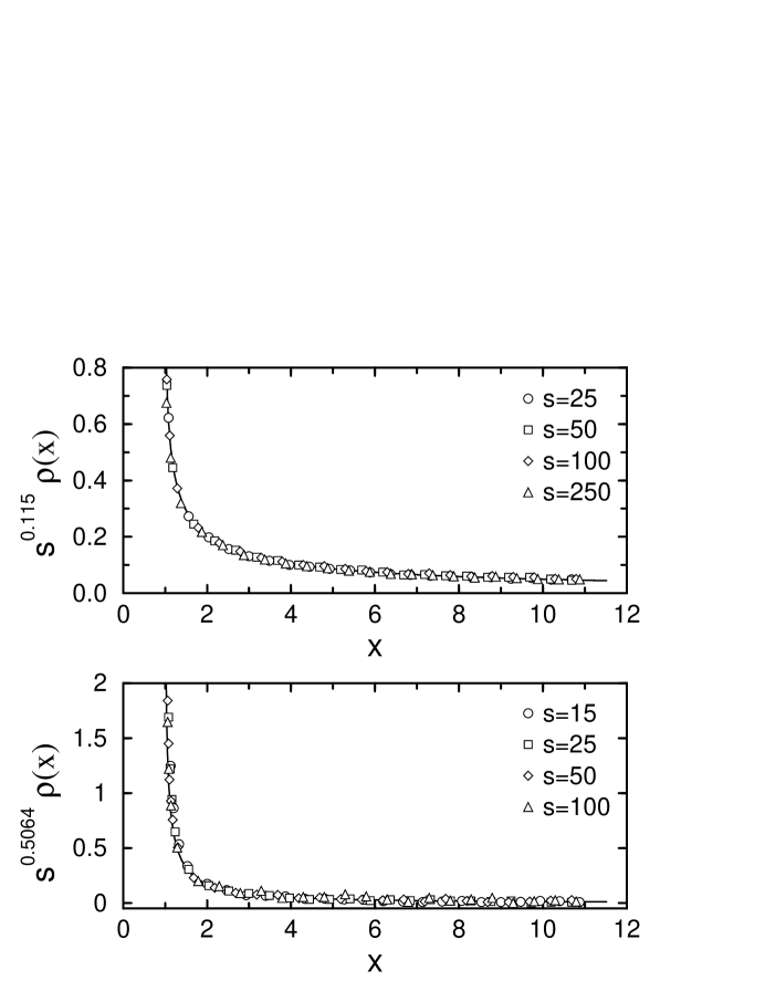
Figure 7: Scaling of the TRM integrated response function $\rho$ for the $2D$ (above) and the $3D$ (below) Glauber-Ising model at criticality ($T=T_{c}$). The symbols correspond to different waiting times. The full curve is the local scale invariance prediction (5.47) for $\rho(t,s)$. The data are from [58].

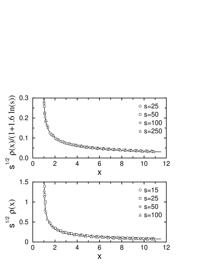
Figure 8: Scaling of the TRM integrated response function $\rho$ for the low-temperature Glauber-Ising model in $2D$ (above) at $T=1.5$ and in $3D$ at $T=3$ (below). The symbols correspond to different waiting times. The full curve is obtained from (5.47). The data are from [58].

Clearly, from (5.47) we expect a data collapse if $s^{a}\rho(t,s)$ is plotted against $x=t/s$. In figure 7 Monte Carlo data at criticality are shown and scaling is indeed seen to hold. Furthermore, upon adjusting the normalization $r_{0}$, there is complete agreement between the data and eq. (5.47). Similarly, data for $T<T_{c}$ are shown in figure 8. While the expected scaling of $s^{1/2}\rho(t,s)$ as a function of $x=t/s$ works well in $3D$, that is not the case in two dimensions. However, recall that analytical calculations [10] on the scaling of the response function in the spirit of the OJK approximation rather suggest in two dimensions the presence of logarithmic corrections $\rho(t,s)\simeq s^{-1/2}\ln(s)f(t/s)$. Therefore, the following ansatz for the $2D$ Glauber-Ising model [58]

$$\rho(t,s)=s^{-1/2}\left(r_{0}+r_{1}\ln s\right)E\left(\frac{t}{s}\right)$$ (5.49)

appears natural, where $r_{0,1}$ are non-universal constants and $E=E(x)$ is a scaling function. Indeed, a satisfactory scaling is found this way, as can be seen from figure 8. It has been checked that the same kind of scaling holds in the entire low-temperature phase, where $r_{0}$ and $r_{1}$ depend on $T$ [58]. Furthermore, the form of the scaling functions thus obtained are again in perfect agreement with the prediction eq. (5.47) of local scale invariance, for both $2D$ and $3D$.

2. Second, eq. (5.38) has been tested extensively in the exactly solvable kinetic spherical model with a non-conserved order parameter, for $d>2$ space dimensions. The kinetic spherical model may be introduced as a spin model [28, 47, 117, 17, 24, 88] with Hamiltonian ${\cal H}=-\sum_{i,j}J_{i,j}S_{i}S_{j}$, where the $J_{i,j}$ are coupling constants and the $S_{i}$ are real variables subject to the spherical constraint

$$\sum_{i}S_{i}^{2}={\cal N}$$ (5.50)

where the sum runs over the entire lattice and $\cal N$ is the number of sites. The dynamics of the model is generated through a stochastic Langevin equation

$$\frac{{\rm d}S_{\boldsymbol{r}}}{{\rm d}t}=-\frac{\delta{\cal H}[S]}{\delta S_{\boldsymbol{r}}}-(2d+\mathfrak{z}(t))S_{\boldsymbol{r}}+\eta_{\boldsymbol{r}}(t)$$ (5.51)

where the Gaussian white noise $\eta_{\boldsymbol{r}}(t)$ has the correlation

$$\langle\eta_{\boldsymbol{r}}(t)\eta_{\boldsymbol{r}^{\prime}}(t^{\prime})\rangle=2T\delta_{\boldsymbol{r},\boldsymbol{r}^{\prime}}\delta(t-t^{\prime})$$ (5.52)

and $\mathfrak{z}(t)$ is determined by satisfying the spherical constraint. Alternatively, the same model may be studied as the $n\to\infty$ limit of the coarse-grained O($n$) vector model using field theory methods, see [12, 23, 66, 82, 16].

In many studies, the short-ranged spherical model with only nearest-neighbour interactions $J_{i,j}$ and an infinite-temperature initial state without any correlations was considered [66, 82, 28, 47, 117, 24]. Exact results for the two-time autocorrelators and autoresponse functions were found. Writing the two-time autoreponse function in the scaling limit as $R(t,s)=(4\pi s)^{-d/2}f_{R}(t/s)$, one has in the ordered phase ($T<T_{c}$) [82, 47] (here and below, we always take $t>s$ or $x>1$)

$$f_{R}(x)=x^{d/4}\,(x-1)^{-d/2}$$ (5.53)

for all values of $d>2$. At the critical point ($T=T_{c}$) one has [66, 47]

$$f_{R}(x)=\left\{\begin{array}[]{ll}x^{1-d/4}(x-1)^{-d/2}&\!\!~{};~{}\mbox{\rm if $2<d<4$}\\ (x-1)^{-d/2}&\!\!~{};~{}\mbox{\rm if $4<d$}\end{array}\right.$$ (5.54)

and both results are in full agreement, upon identification of exponents, with eq. (5.38). The second expression of (5.54) corresponds to the mean-field case and coincides with the result found for a free Gaussian field [26], as expected. We point out that the form of the correlation scaling functions depends strongly on $d$ and on whether $T<T_{c}$ or $T=T_{c}$ since the behaviour of the fluctuation-dissipation ratio $X(t,s)$ is different [47] in each of the three cases considered so far.

More recently, these results have been generalized in two directions. First, the two-time autocorrelation and autoresponse functions were calculated exactly in the kinetic spherical model with spatially long-range interactions, of the form [17]

$$J_{i,j}=J(\boldsymbol{r}_{ij})=J_{0}|\boldsymbol{r}_{ij}|^{-d-\sigma}\left({\sum_{j}}^{\prime}|\boldsymbol{r}_{ij}|^{-d-\sigma}\right)^{-1}$$ (5.55)

where ${\sum_{j}}^{\prime}$ runs over all sites $j\neq i$, $\boldsymbol{r}_{ij}$ is the distance between sites $i$ and $j$, $J_{0}$ is a constant and $\sigma$ is a free parameter. For $d>2$ and $\sigma>2$, one recovers the short-ranged spherical model discussed above. On the other hand, if either (i) $d>2$ and $0<\sigma<2$ or else (ii) $d\leq 2$ and $0<\sigma<d$ the model has an equilibrium phase transition at a non-vanishing $T_{c}$ between an ordered and a paramagnetic phase [17]. In this case and below criticality ($T<T_{c}$), the dynamical exponent $z=\sigma$ and the response function is in the aging scaling limit [17]

$$R(t,s)=r_{0}\,(t/s)^{d/(2\sigma)}(t-s)^{-d/\sigma},$$ (5.56)

which again fully confirms eq. (5.38). One identifies the exponents $a=d/\sigma-1$ and $\lambda_{R}=d/2$ in the ordered phase. We are not aware of any published results on $R$ in this model at criticality.

Second, the case of nearest-neighbour interactions but with long-ranged correlations characterized by the form

$$C_{\rm ini}(\boldsymbol{r})\sim|\boldsymbol{r}|^{-d-\alpha}$$ (5.57)

of the spin-spin correlator in the initial state has been studied [82, 12, 23, 88]. The uncorrelated initial state considered above is recovered as the special case $\alpha=0$. Indeed, the effect of initial correlations is only notable in the long-time behaviour if $\alpha<0$. In the ordered phase ($T<T_{c}$), the exact autoresponse function is in the scaling limit $R(t,s)=(4\pi s)^{-d/2}f_{R}(t/s)$, where [82, 88]

$$f_{R}(x)=x^{(d+\alpha)/4}\,(x-1)^{-d/2}$$ (5.58)

in complete agreement with (5.38). For $\alpha=0$, eq. (5.53) is reproduced. At criticality ($T=T_{c}$), five distinct regimes of non-equilibrium critical dynamics exist [88]. These are distinguished by the values of $d$ and $\alpha$ as listed in table 8 which also gives the values of the required non-equilibrium exponents.

Table 8: Some non-equilibrium exponents of the kinetic spherical model with short-ranged interactions and correlated initial conditions of the form (5.57), for the five distinct regimes I,…,V at criticality ($T=T_{c}$) and also in the ordered phase ($T<T_{c}$). Here $D=d+\alpha+2$.

Regime	conditions			$\digamma$	$a$	$z$	$\lambda_{R}$
I	$2<d<4$	$2<D<4$		$\alpha/4-1/2$	$d/2-1$	2	$d-\alpha/2-1$
II	$4<d$	$2<D<4$		$(d+\alpha)/4-1/2$	$d/2-1$	2	$(d-\alpha)/2+1$
III	$2<d<4$	$4<D$		$1-d/4$	$d/2-1$	2	$3d/2-2$
IV	$4<d$	$4<D$	$\alpha>-2$	$0$	$d/2-1$	2	$d$
V	$4<d$	$4<D$	$\alpha<-2$	$0$	$d/2-1$	2	$d$
$T<T_{c}$	$2<d$			$(d+\alpha)/4$	$d/2-1$	2	$(d-\alpha)/2$

The autoresponse function is $R(t,s)=(4\pi)^{-d/2}s^{-1-a}f_{R}(t/s)$ in all five regimes where [88]

$$f_{R}(x)=x^{\digamma}\,(x-1)^{-d/2}$$ (5.59)

and the values of the exponent $\digamma$ can be read off from table 8. Once more we find complete agreement with eq. (5.38). The results quoted in eq. (5.54) are reproduced in the critical regimes III and IV. Again, the behaviour of the autocorrelations differs widely between the five regimes as discussed in detail in [88].

3. Recently, the off-equilibrium response and correlation functions of the O($n$)-symmetric vector model with a non-conserved order parameter (model A in the terminology of [51]) and a fully disordered initial state were calculated in one-loop order in $d=4-\varepsilon$ dimensions [16]. From earlier calculations of correlators and responses with the initial state at criticality [66], the critical exponents

$$z=2+{\rm O}\left(\varepsilon^{2}\right)\;\;,\;\;a=\frac{d}{2}-1+{\rm O}\left(\varepsilon^{2}\right)\;\;,\;\;\lambda_{R}=d-\frac{\varepsilon}{2}\frac{n+2}{n+8}+{\rm O}\left(\varepsilon^{2}\right)$$ (5.60)

were already known. At criticality, the autoresponse function is in the scaling limit [16]

$$R(t,s)=r_{0}\left(\frac{t}{s}\right)^{\frac{\varepsilon}{4}\frac{n+2}{n+8}}\,\left(t-s\right)^{-d/2}+{\rm O}\left(\varepsilon^{2}\right)$$ (5.61)

which again agrees, to first order in $\varepsilon$, with the prediction (5.38). It would be extremely interesting to see whether this agreement can be extended to higher orders in the $\varepsilon$-expansion. We are not aware of any results on $R(t,s)$ in the low-temperature phase.

4. A particularly simple textbook system which reproduces eq. (5.38) is the free random walk, see [26]. It is described in the continuum through the following Langevin equation for $y(t)$ and the correlator of the Gaussian white noise $\eta$

$$\frac{{\rm d}y(t)}{{\rm d}t}=\eta(t)\;\;,\;\;\langle\eta(t)\eta(s)\rangle=2T\delta(t-s)$$ (5.62)

The autocorrelation function and the autoresponse function are readily found [26]

$$C(t,s) = \langle y(t)y(s)\rangle\hskip 8.82036pt=2T\min(t,s)$$

$$R(t,s) = \left.\frac{\delta\langle y(t)\rangle}{\delta h(s)}\right|_{h=0}=\frac{1}{2T}\langle y(t)\eta(s)\rangle=\Theta(t-s)$$ (5.63)

and do satisfy the scaling fom (5.32). The system is out of equilibrium since the fluctuation-dissipation ratio $X(t,s)=1/2$. The exact expression for $R(t,s)$ matches eq. (5.38) with the exponents $a=-1$ and $\lambda_{R}/z=0$.

5. Having studied so far simple ferromagnets, we now consider the spherical model spin glass [28] as a very simple example of a disordered system. The Hamiltonian ${\cal H}=-\sum_{(i,j)}J_{i,j}S_{i}S_{j}$ describes nearest-neighbour interactions between the spherical spins subject to the constraint (5.50). The couplings $J_{i,j}$ are independently distributed quenched random variables with zero mean and variance inversely proportional to the number of sites $\cal N$. For uniform initial conditions, the mean-field two-time autoresponse function is in the scaling limit [28]

$$R(t,s)=r_{0}\left(\frac{t}{s}\right)^{3/4}\,(t-s)^{-3/2}$$ (5.64)

which again agrees with (5.38). Could this be a hint that the form (5.38) for $R(t,s)$ might also hold for glassy systems ? In fact, the result (5.64) coincides with eq. (5.54) for $d=3$. This is a consequence of the known [117] similarity between the $3D$ spherical ferromagnet and the mean-field spherical spin glass. Therefore, although the result (5.64) may appear suggestive, it is not yet clear at all whether or not the predictions (5.38,5.47) of local scale invariance may be reproducible in physically interesting glassy systems.

6. The tests described so far all concerned the autoresponse function $R(t,s)$. Spatio-temporal responses $R(t,s;\boldsymbol{r})$ have so far only been tested in the exactly solvable spherical model. For short-ranged interactions, the dynamical exponent $z=2$ and from local scale invariance (or Schrödinger invariance in this case) we expect (5.44) to hold. Indeed, this had been checked long ago for a disordered initial state both at and below $T_{c}$ [66, 82, 53] and recently for an initial state with the long-range correlations of the form (5.57), again both at and below $T_{c}$ [88]. To leading order in the $\varepsilon$-expansion, eq. (5.44) also holds in the O($n$)-model [16]. Tests of the spatio-temporal response (5.42) in the Glauber-Ising model both below and at criticality are currently being performed and will be reported elsewhere.

Summarising, we have seen that the form eq. (5.38) of the two-time autoreponse function has been reproduced in a considerable variety of non-equilibrium ferromagnetic spin systems with a non-conserved order parameter. The examples for which (5.38) has so far be seen to hold suggest its validity independently of the following characteristics of specific models, namely (see also note added)

1. the value of the dynamical exponent $z$.

2. the value of the space dimension, provided $d>1$.

3. the number of components of the order parameter and the global symmetry group.

4. the spatial range of the spin interactions.

5. the presence of spatial long-range correlations in the initial state.

6. the value of $T$, in particular whether $T<T_{c}$ or $T=T_{c}$, provided $T_{c}>0$.

The response functions of different universality classes are only distinguished by the values of the exponents $a$ and $\lambda_{R}/z$.

Clearly, further tests in different models will be most useful to either confirm further or else invalidate this conjecture. On the other hand, as yet there are only few tests of the full spatio-temporal response (5.42). At present, there is no prediction from local scale invariance for the two-time correlation functions in non-equilibrium dynamical scaling.

Finally, we comment on some examples where eq. (5.38) does not hold. From the exact solution of the $1D$ Glauber-Ising model at $T=0$ one has in the aging regime $R(t,s)=[2\pi^{2}s(t-s)]^{-1/2}$ [46, 76]. For the $2D$ XY model in the critical low-temperature phase, one has in the spin-wave approximation $R(t,s)\sim s^{-1-\eta/2}f_{R}(t/s)$ with $f_{R}(x)=[(x+1)^{2}/x]^{\eta/4}(x-1)^{-1-\eta/2}$ [11]. Here $\eta=\eta(T)$ is the usual equilibrium temperature-dependent exponent, see [11, 34, 116, 19] and references therein. It is well-established, however, that in these models already the growth law $L=L(t)$ is unusual: the generic description which assumes that energy dissipation is dominated by the motion of single defect structures at the scale $L=L(t)$ no longer applies here [95, 14]. From that perspective, it is not too surprising that also the form of the scaling functions should be non-generic in these models. We shall come back elsewhere to the question whether these systems may or may not be treated by some form of local scale invariance [89].

5.3 Equilibrium critical dynamics

Having discussed the local scaling of the response function out of equilibrium, we now briefly turn towards the case of equilibrium critical dynamics. It will be of interest to compare the predictions of local scale invariance as introduced here with those obtained from dynamical conformal invariance [18].

Consider a spin system at its equilibrium critical point. Two-time correlation functions and response functions can be defined as before, see eq. (5.28). However, and in contrast to the non-equilibrium case, time translation invariance is expected to hold and we should have

$$C=C(t-s;\boldsymbol{r})\;\;,\;\;R=R(t-s;\boldsymbol{r})$$ (5.65)

The response functions should transform covariantly under local scale transformations, as originally proposed in [18]. In consequence, carrying over the treatment of section 4, $R$ is again given by eq. (5.42), viz.

$$R(\tau;\boldsymbol{r})=\langle\phi(\tau,\boldsymbol{r})\widetilde{\phi}(0;\boldsymbol{0})\rangle=\tau^{-2x_{1}/z}\Phi\left(r\tau^{-1/z}\right)$$ (5.66)

but with the additional constraint $x_{1}=x_{2}$ coming from time translation invariance (alternatively, this constraint may be written as $\lambda_{R}/z=1+a$). The scaling function $\Phi(u)$ is given as before by eq. (4.16). The constraints discussed above in section 5.2 for the non-equilibrium response also apply.

Since at equilibrium the fluctuation-dissipation theorem

$$T_{c}R(\tau;\boldsymbol{r})=-\frac{\partial}{\partial\tau}C(\tau;\boldsymbol{r})$$ (5.67)

holds [19, 71], where $\tau=t-s$, the scaling form of the two-time correlator may be given as well. Integrating, we have

$$C(t;\boldsymbol{r})=C(0;\boldsymbol{r})-T_{c}z\>r^{z-2x_{1}}\int_{rt^{-1/z}}^{\infty}\!{\rm d}u\,u^{2x_{1}-z-1}\Phi(u)$$ (5.68)

Here $C(0;\boldsymbol{r})=\langle\phi(t,\boldsymbol{r})\phi(t,\boldsymbol{0})\rangle$ is the equal-time correlator, which is $t$-independent, because time translation invariance holds at the equilibrium critical point.

We point out that the exponent $x_{1}$ which enters (5.68) is not a static critical exponent. Rather, it is related to the static scaling dimension $x_{1}^{\rm(g)}$ by

$$2x_{1}^{\rm(g)}=2x_{1}-z$$ (5.69)

For example, for a $2D$ critical point, the $x_{1}^{\rm(g)}$ are the scaling dimensions which can be obtained from the representations of the Virasoro algebra [8]. In terms of these, we have, with $u=rt^{-1/z}$

$$R(t;\boldsymbol{r}) = t^{-1-2x_{1}^{\rm(g)}/z}\Phi\left(rt^{-1/z}\right)$$ (5.70)

$$C(t;\boldsymbol{r}) = C(0;\boldsymbol{r})-T_{c}z\>r^{-2x_{1}^{\rm(g)}}\int_{u}^{\infty}\!{\rm d}w\,w^{2x_{1}^{\rm(g)}-1}\Phi(w)$$ (5.71)

Because of the known behaviour of $\Phi(w)$ at the $w\to 0$ and $w\to\infty$ boundaries, it is easy to see that the integral in (5.71) is convergent if $x_{1}^{\rm(g)}>0$ and $z>0$. Since we are at criticality, we expect $C(0;\boldsymbol{r})\sim r^{-2x_{1}^{\rm(g)}}$ and finally obtain

$$C(t;\boldsymbol{r})=r^{-2x_{1}^{\rm(g)}}\left(C_{0}+C_{1}\int_{0}^{u}\!{\rm d}w\,w^{2x_{1}^{\rm(g)}-1}\Phi(w)\right)\;\;,\;\;u=rt^{-1/z}$$ (5.72)

where $C_{0,1}$ are non-universal normalization constants.

We now compare the scaling form (5.70) with the prediction of dynamical conformal invariance for a non-conserved order parameter $R(t,r)\sim t^{-1-2x/z}\exp(-r^{z}/t)$ [18], up to suppressed non-universal constants. In our theory, we have found a simple exponential scaling function in two cases: (i) $z=2$ with $\beta_{1}+\gamma_{1}={\cal M}/2\neq 0$ and (ii) $z=1$ with $\beta_{1}+\gamma_{1}=0$. In these special cases, the two-time correlator takes the following form: in the case $z=2$, ${\cal M}\neq 0$

$$C(t,\boldsymbol{r})=r^{-2x_{1}^{\rm(g)}}\left[C_{0}+C_{1}\,\gamma\left(x_{1}^{\rm(g)},\frac{\cal M}{2}\frac{r^{2}}{t}\right)\right]$$ (5.73)

and in the case $z=1$, $\beta_{1}+\gamma_{1}=0$

$$C(t,\boldsymbol{r})=r^{-2x_{1}^{\rm(g)}}\left[C_{0}+C_{1}\,\gamma\left(2x_{1}^{\rm(g)},2\gamma_{1}\frac{r}{t}\right)\right]$$ (5.74)

respectively. Here $\gamma(a,z)$ is an incomplete gamma function, see eqs. (6.5.4), (6.5.29) in [1] and $C_{0,1}$ are normalization constants. In all other cases, the scaling functions will take a form quite distinct from these two examples, see figures 1 and 2. We recall that the fundamental hypothesis of dynamical conformal invariance was conformal invariance in space [18] and not in time, as we have assumed throughout this paper.

Tests of the consequences (5.70,5.72) of the hypothesis of local scale invariance in equilibrium critical dynamics in specific models would be most welcome.

6 Conclusions

Our starting point has been the heuristic idea that it might be possible to extend strongly anisotropic or dynamical scaling from mere dilatation invariance with a given anisotropy exponent $\theta$ (or dynamical exponent $z$) to a larger dynamical symmetry involving local scale transformations with a space-time-dependent dilatation factor. We have studied this idea by seeking confirmation on the purely phenomenological level of being able to reproduce certain two-point function in the context of specific models. The agreement found provides evidence in favour of, but does not prove, this hypothesis of local scale invariance.

In attempting to construct local scale transformations for an arbitrary anisotropy exponent $\theta$, we have tried to follow the two known cases of conformal and Schrödinger invariance as closely as possible. The common feature of these groups is the presence of conformal transformations in time and we have made this the central assumption in our formulation of local scale invariance.

In carrying out the construction of infinitesimal local scale transformations, we have seen that there exist two types, the first one (Typ I) being related to strongly anisotropic equilibrium systems, while the second one (Typ II) describes systems with time-dependent dynamical scaling. The main properties of local scale invariance when applied to quasiprimary operators are collected in table 2. Conformal invariance and Schrödinger invariance are recovered as special cases, for $\theta=1$ and $\theta=2$, respectively. On the other hand, if $\theta\neq 1,2$, the generators only close into a Lie algebra on certain states only and thus form a weak Lie algebra.

Local scale transformations form a (weak) dynamic symmetry group of the equation of motion ${\cal S}\psi=0$ of certain, in general non-local, free-field theories (see table 2 for the precise form of $\cal S$).

In addition, two-point functions formed from quasiprimary operators satisfy certain linear (fractional) differential equations, from which the form of these two-point functions can be determined.

Indeed, these explicit predictions (see eqs. (4.23,4.25) for Typ I with $N=2/\theta\in\mathbb{N}$ and eq. (4.16) for Typ II) allow for a test of the applicability of our notion of local scale invariance in concrete models. These tests have been performed in two different settings:

1. Uniaxial Lifshitz points are a classic example of a strongly anisotropic equilibrium system. The form of the spin-spin correlator at the first-order Lifshitz points in both the ANNNS model and the $3D$ ANNNI model and also at the second-order Lifshitz point in the ANNNS model agrees fully with local scale invariance, for $\theta\simeq\frac{1}{2}$ and $\theta=\frac{1}{3}$, respectively [55, 90].

2. Dynamical scaling occurs in the aging behaviour of simple ferromagnets which undegoes phase-ordering kinetics or non-equilibrium critical dynamics. We found a particularly simple scaling form of the two-time autoresponse function in the aging regime

   $$R(t,s) = \left.\frac{\delta\langle\sigma(t)\rangle}{\delta h(s)}\right|_{h=0}=s^{-1-a}f_{R}(t/s)$$

   $$f_{R}(x) = r_{0}\,x^{A}(x-1)^{B}$$ (6.1)

   where the values of the exponents $A$ and $B$ can be matched to known dynamical exponents, see section 5.2. This form can be reproduced in a large variety of models, with the dynamical exponent $z$ taking values both below and above 2, notably in the $2D$ and $3D$ Glauber-Ising models, the O($n$)-symmetric kinetic model A to first order in the $\varepsilon$-expansion, several variants of the kinetic spherical model with non-conserved order parameter and brownian motion [58, 16, 47, 17, 88, 26].

   The form (2) for the scaling function $f_{R}(x)$ is likely to be very robust and of broad validity, see section 5.2.

We stress that the $3D$ ANNNI model and the $2D$ and $3D$ Glauber-Ising models cannot be expressed as free-field theories. This renders the confirmation of local scale invariance in these models non-trivial.

Technically, our results depend on the construction of commuting fractional derivatives. That property was essential in the derivation of the fractionall differential equations satisfied by the scaling function of the two-point function. However, these differential equations themselves do not depend on any other property of the fractional derivatives. On the other hand, a specific choice must be made for the fractional derivative if an explicit solution is requested. At present, there is not yet any test available which would inform us whether the specific form used in this work or else any of the known alternatives is realized in the context of local scale invariance.

The possibility of local scale invariance has recently been discussed (under the name of reparametrization invariance) in the aging of certain glassy systems, where the covariance of correlators and response functions was studied [69, 21]. In the models studied there, the scaling dimensions $x_{\phi}=0$ of the order parameter $\phi$ and $x_{\widetilde{\phi}}=1$ of the response operator $\widetilde{\phi}$ take rather simple values, however. The covariance of non-equilibrium two-time correlators under time reparametrizations also plays a role in a recent study on general constraints on the scaling of these [73]. Finally, a recently introduced model for a fluctuating interface with $z=1$ can be described in the thermodynamic limit in terms of the characters of a conformal field theory [44].

All in all, we have proposed a new type of dynamical symmetry which might generalize usual anisotropic or dynamical scaling. The existing phenomenological confirmations provide evidence for local scale invariance to be realized, at least to a very good approximation, in certain statistical systems. Of course, the theory must be built further and in particular, one would like to be able to show that the field theories underlying these scale-invariant statistical systems indeed satisfy local scale invariance. Work along several of these lines is in progress.

Note added in proof:

For the critical weakly disordered kinetic Ising model with a non-conserved order parameter, Calabrese and Gambassi [118] find, to one-loop order, the response function at vanishing external momentum $\boldsymbol{q}$ to be in full agreement with the prediction of local scale invariance.

Acknowledgements

It is a pleasure to thank L. Berthier, C. Godrèche, H. Hinrichsen, D. Karevski, J.-M. Luck, A. Picone, J. Unterberger and especially M. Pleimling for useful discussions and/or correspondence. Parts of this work were done at the Centro de Física da Matéria Condensada (CFMC) of the Universidade de Lisboa and at the Fachbereich Physik of the Universität Saarbrücken, whom I thank for warm hospitality. Support of the CINES Montpellier (projet pmn2095) is gratefully acknowledged.

Appendix A. On fractional derivatives

Fractional derivation and integration is a well-established topic, see [99, 79, 91, 60] for reviews. However, for a derivative operator $\partial^{a}$ of real order $a$ the commutativity $\partial^{a}\partial^{b}=\partial^{a+b}=\partial^{b}\partial^{a}$ is not trivial. The well-known Riemann-Liouville and Grünwald-Letnikov fractional derivatives do not satisfy it. Since our construction of local scaling operators is built around this property, we shall present here fractional derivatives in a self-contained manner such that commutativity is guaranteed, along with some other simple calculational rules. In particular, the definition used here allows for the solving of fractional differential equations of rational order by series expansion methods. For simplicity, we merely consider functions $f(r)$ of a single variable $r$.

Consider a set $E$ of numbers $e$ such that any $e\in E$ is not a negative integer, $e\neq-(n+1)$ with $n\in\mathbb{N}$. We call such a set an E-set. Let $I$ be some (possibly infinite) positive real interval. We define the $\cal M$-space of generalized functions associated with the E-set $E$

$${\cal M}:={\cal M}_{E}(I,\mathbb{R})=\left\{f:I\subset\mathbb{R}\to\mathbb{R}\left|f(r)=\sum_{e\in E}f_{e}r^{e}+\sum_{n=0}^{\infty}F_{n}\delta^{(n)}(r)\;;f_{e}\in\mathbb{R}\;,F_{n}\in\mathbb{R}\right.\right\}$$ (A1)

where $\delta^{(n)}(r)$ is the $n^{\rm th}$ derivative of the Dirac delta function. The part of $f\in{\cal M}$ parametrized by the constants $f_{e}$ is called the regular part of $f$ and the part parametrized by the $F_{n}$ is call the singular part of $f$. A well-known theorem [42, p. 81] states that any generalized function $f(r)$ concentrated at $r=0$ is indeed given by a finite sum $\sum_{n}F_{n}\delta^{(n)}(r)$. It is understood throughout that only finitely many of the coefficients $F_{n}$ in (A1) are non-vanishing. Furthermore, we assume that the regular part in (A1) converges ‘well enough’ that all ‘reasonable’ operations can be carried out (see Lemma 2 below for a sufficient condition). For example, we could choose $E=\mathbb{N}$ and take $\cal M$ to be the set of analytic functions on $I$. More generally, if we take $E=\mu\mathbb{N}+\lambda$ with $\mu>0$ and $\lambda\neq-(\mu(n+1)+m+1)$ with $n,m\in\mathbb{N}$, ${\cal M}_{E}$ is the space of functions of the form $r^{\lambda}f\left(r^{\mu}\right)$ with $f(r)$ analytic. Although everything here is specified in terms of real numbers, the formal extension to complex-valued functions is immediate.

Definition: Let $a\in\mathbb{R}$, $E$ be an E-set and let $E^{\prime}:=\{e^{\prime}|e^{\prime}=e-a;e\in E\}$. Analogously to (A1) one has the space ${\cal M}^{\prime}={\cal M}_{E^{\prime}}$. An operator $\partial^{a}:{\cal M}\to{\cal M}^{\prime}$ is called a derivative of order $a$, iff it satisfies the properties:

i) $$\partial^{a}\left(\lambda f(r)+\mu g(r)\right)=\lambda\partial^{a}f(r)+\mu\partial^{a}g(r)\;\;\forall\lambda,\mu\in\mathbb{R}\;\mbox{\rm and all }f,g\in{\cal M}$$

ii) $$\partial^{a}r^{e}=\frac{\Gamma(e+1)}{\Gamma(e-a+1)}r^{e-a}+\sum_{n=0}^{\infty}\delta_{a,e+n+1}\Gamma(e+1)\delta^{(n)}(r)$$ (A2)

iii) $$\partial^{a}\delta^{(n)}(r)=\frac{r^{-1-n-a}}{\Gamma(-a-n)}+\sum_{m=0}^{\infty}\delta_{a,m}\delta^{(n+m)}(r)$$

where $\Gamma(x)$ is the Gamma function. In particular, it follows from (A2) that the prefactor for any monomial $r^{-n-1}$ with $n\in\mathbb{N}$ indeed vanishes. For our purposes, we may consider the set $E^{\prime}$ therefore also as an E-set and ${\cal M}^{\prime}$ as an ${\cal M}$-space.

In particular, it is implied that $\partial^{a}$ can be applied term-by-term to any function $f\in{\cal M}$. Often, we shall also write $\partial^{a}=\partial_{r}^{a}$ if we want to specify explicitly the variable $r$ on which $\partial^{a}$ is supposed to act. We point out that $\partial^{a}$ is not defined on negative integer powers $r^{-n-1}$ with $n\geq 0$.

In order to show that this definition is not empty, recall the definition of fractional derivatives as given by Gelfand and Shilov [42, p. 115]. For the real line, they consider the generalized function

$$r_{+}^{\alpha}:=\left\{\begin{array}[]{ll}r^{\alpha}&;~{}~{}r>0\\ 0&;~{}~{}r\leq 0\end{array}\right.$$ (A3)

and for generalized functions concentrated on the half-line $r\geq 0$, they define

$$\partial^{a}f(r):=f(r)*\frac{r_{+}^{-a-1}}{\Gamma(-a)}=\frac{1}{\Gamma(-a)}\int_{0}^{r}\!{\rm d}\rho\>f(\rho)\left(r-\rho\right)^{-a-1}$$ (A4)

It is understood that the integral must be regularized [42]. The conditions (A2) are immediately verified [42], using $\int_{0}^{1}\!{\rm d}t\,t^{a-1}(1-t)^{b-1}=\Gamma(a)\Gamma(b)/\Gamma(a+b)$ and analytic continuation. For comparison with the Riemann-Liouville/Grünwald-Letnikov/Marchaud fractional derivatives $D^{a}={}_{0}D_{r}^{a}$, we recall that $D^{a}r^{e}=(\Gamma(e+1)/\Gamma(e-a+1))\,r^{e-a}$ [99, 79, 91, 60]. The singular terms which arise in the definition (A2) are absent.

The practical interest of the definition (A2) comes from the following simple rules for calculation.

Lemma 1: If $E$ is an E-set, $\cal M$ the associated $\cal M$-space, $f\in{\cal M}$ and $\partial^{a}$ the derivative of order $a$ such that all $\partial^{a}f$ considered below exist, one has on ${\cal M}$

$$\partial^{a+b}f(r) = \partial^{a}\partial^{b}f(r)=\partial^{b}\partial^{a}f(r)$$ (A5)

$$\left[\partial^{a},r\right]f(r) = a\partial^{a-1}f(r)$$ (A6)

$$\partial_{r}^{a}f(\lambda r) = \lambda^{a}\partial_{\lambda r}^{a}f(\lambda r)$$ (A7)

$$\partial_{\lambda r}^{a}f(r) = \lambda^{-a}\partial_{r}^{a}f(r)$$ (A8)

where $\lambda>0$ is a real constant. If $f$ is analytic without singular terms and $g\in{\cal M}$, one has

$$\partial^{a}\left(f(r)g(r)\right)=\sum_{\ell=0}^{\infty}\left(\begin{array}[]{c}a\\ \ell\end{array}\right)\frac{{\rm d}^{\ell}f(r)}{{\rm d}r^{\ell}}\,\partial^{a-\ell}g(r)$$ (A9)

where ${\rm d}^{\ell}/{\rm d}r^{\ell}$ are ordinary derivatives of integer order $\ell$. These rules are the natural generalizations of the familiar properties of the usual derivative. The commutator $[.,.]$ is defined as usual. Well-known fractional derivatives such as the Riemann-Liouville, Gründwald-Letnikov or Marchaud fractional derivatives satisfy the commutativity relation (A5) only if further conditions are imposed on $a$ and $b$ or on the function $f(r)$ [99, 79, 91] (see also the example (A14) below). On the other hand, (A5) does hold for the Gelfand-Shilov definition (A4) [42, 91], the Weyl fractional derivative [79] and for the recent complex multivalued definition presented in [115]. The generalized Leibniz rule (A9) is usually proven for both $f,g$ analytic [99] or infinitely often differentiable [91]. In [79], $f$ is analytic and $g\in{\cal M}_{M}$, with the E-set $M=\mathbb{N}+\mu$, $\mu>-1$ (logarithms are also admitted). Generalized (and simpler) Leibniz rules based on the convolution product were discussed in [70].

So far, the definition of $\partial^{a}$ was performed for variables $r>0$ (and we should have written $r_{+}^{e}$ instead of $r^{e}$ everywhere). We may use (A7) with $\lambda$ negative to formally extend the definition of $\partial^{a}$ to any value of $r\neq 0$. Then (A5,A6,A8) remain valid.

Proof: We show that the rules of the lemma can be reduced to the basic properties (A2). In order to prove (A5), we consider separately two cases. Let

$${\rm ind}_{b\not\in\mathbb{N}}:=\left\{\begin{array}[]{ll}1&\mbox{\rm~{}~{};~{} if~{}~{} $b\not\in\mathbb{N}$}\\ 0&\mbox{\rm~{}~{};~{} if~{}~{} $b\in\mathbb{N}$}\end{array}\right.$$ (A10)

First, consider

$$\partial^{a}\partial^{b}\delta(r)\;=\;\partial^{a}\left(\frac{r^{-1-b}}{\Gamma(-b)}+\sum_{m\in\mathbb{N}}\delta_{b,m}\delta^{(m)}(r)\right)$$

$$= \frac{{\rm ind}_{b\not\in\mathbb{N}}}{\Gamma(-b)}\left(\frac{\Gamma(-b)r^{-1-b-a}}{\Gamma(-b-a)}+\sum_{n\in\mathbb{N}}\delta_{a,-b+n}\Gamma(-b)\delta^{(n)}(r)\right)+\sum_{m\in\mathbb{N}}\delta_{b,m}\left(\frac{r^{-1-m-a}}{\Gamma(-a-m)}+\sum_{n\in\mathbb{N}}\delta_{a+b,n}\delta^{(n)}(r)\right)$$

$$= \frac{1}{\Gamma(-b-a)}r^{-1-b-a}+\sum_{n\in\mathbb{N}}\delta_{a+b,n}\delta^{(n)}(r)\;=\;\partial^{a+b}\delta(r)$$

and this also implies commutativity on $\delta^{(n)}(r)=\partial^{n}\delta(r)$. Second, we have

$$\partial^{a}\partial^{b}r^{e} = \partial^{a}\left(\frac{\Gamma(e+1)}{\Gamma(e-b+1)}r^{e-b}+\sum_{n\in\mathbb{N}}\delta_{b,e+n+1}\Gamma(e+1)\delta^{(n)}(r)\right)$$

$$= {\rm ind}_{b-e-1\not\in\mathbb{N}}\frac{\Gamma(e+1)}{\Gamma(e-b+1)}\left(\frac{\Gamma(e-b+1)}{\Gamma(e-a-b+1)}r^{e-b-a}+\sum_{m\in\mathbb{N}}\delta_{a,e-b+m+1}\Gamma(e-b+1)\delta^{(m)}(r)\right)$$

$$+\sum_{n\in\mathbb{N}}\delta_{b,e+n+1}\left(\frac{\Gamma(e+1)}{\Gamma(-a-n)}r^{-1-n-a}+\sum_{m\in\mathbb{N}}\delta_{a,m}\Gamma(e+1)\delta^{(n+m)}(r)\right)$$

$$= \frac{\Gamma(e+1)}{\Gamma(e-b-a+1)}r^{e-b-a}+\sum_{m\in\mathbb{N}}\delta_{a+b,e+m+1}\Gamma(e+1)\delta^{(m)}(r)$$

$$= \partial^{a+b}r^{e}$$

Having thus checked the claim on the ‘basis set’ spanned by $r^{e}$ and $\delta^{(n)}$ it holds on $\cal M$ by linear superposition. Clearly $\partial_{r}^{a}\partial_{r}^{b}f=\partial_{r}^{b}\partial_{r}^{a}f$. In the sequel we shall need the identities

$$r\delta^{(n)}(r)=-n\delta^{(n-1)}(r)\;\;,\;\;\delta^{(n)}(\lambda r)=\lambda^{-n-1}\delta^{(n)}(r)$$ (A11)

To prove (A6), consider

$$\left[\partial_{r}^{a},r\right]r^{e}=\partial_{r}^{a}r^{e+1}-r\partial_{r}^{a}r^{e}$$

$$= \left(\frac{\Gamma(e+2)}{\Gamma(e-a+2)}-\frac{\Gamma(e+1)}{\Gamma(e-a+1)}\right)r^{e-a+1}$$

$$+\sum_{n=0}^{\infty}\delta_{a,e+n+2}\Gamma(e+2)\delta^{(n)}(r)-\sum_{n=0}^{\infty}\delta_{a,e+n+1}\Gamma(e+1)r\delta^{(n)}(r)$$

$$= \frac{a\Gamma(e+1)}{\Gamma(e+1-(a-1))}r^{e-(a-1)}+a\sum_{n=0}^{\infty}\delta_{a-1,e+n+1}\Gamma(e+1)\delta^{(n)}(r)$$

$$= a\partial_{r}^{a-1}r^{e}$$

where in the third line the first identity (A11) was used. Next,

$$\left[\partial^{a},r\right]\delta^{(p)}(r) = -p\partial^{a}\delta^{(p-1)}(r)-r\partial^{a}\delta^{(p)}(r)$$

$$= -\left(\frac{p}{\Gamma(-a-p+1)}+\frac{1}{\Gamma(-a-p)}\right)r^{-p-a}-\sum_{m=0}^{\infty}\delta_{a,m}\left(p\delta^{(p-1+m)}(r)+r\delta^{(p+m)}(r)\right)$$

$$= \frac{a}{\Gamma(-(a-1)-p)}r^{-1-p-(a-1)}+a\sum_{m=0}^{\infty}\delta_{a,m}\delta^{(p+a-1)}(r)\;=\;a\partial_{r}^{a-1}\delta^{(p)}(r)$$

where the first identity (A11) was used again. Having checked (A6) on $r^{e}$ and $\delta^{(n)}$, it holds on $\cal M$ by linear superposition. For (A7), we set $s=\lambda r$ and use the second identity (A11). Then

$$\partial_{r}^{a}f(\lambda r) = \partial_{r}^{a}\left(\sum_{e\in E}f_{e}\>(\lambda r)^{e}+\sum_{n=0}^{\infty}F_{n}\delta^{(n)}(\lambda r)\right)=\partial_{r}^{a}\left(\sum_{e\in E}\lambda^{e}f_{e}\>r^{e}+\sum_{n=0}^{\infty}\lambda^{-n-1}F_{n}\delta^{(n)}(r)\right)$$

$$= \sum_{e\in E}\lambda^{e}f_{e}\Gamma(e+1)\left(\frac{r^{e-a}}{\Gamma(e-a+1)}+\sum_{m=0}^{\infty}\delta_{a,e+m+1}\delta^{(m)}(r)\right)$$

$$+\sum_{n=0}^{\infty}F_{n}\lambda^{-n-1}\left(\frac{r^{-1-n-a}}{\Gamma(-a-n)}+\sum_{m=0}^{\infty}\delta_{a,m}\delta^{(n+m)}(r)\right)$$

$$= \lambda^{a}\left(\sum_{e\in E}f_{e}\partial_{\lambda r}^{a}(\lambda r)^{e}+\sum_{n=0}^{\infty}F_{n}\partial_{\lambda r}^{a}\delta^{(n)}(\lambda r)\right)\;=\;\lambda^{a}\partial_{s}^{a}f(s)$$

For the forth relation (A8), let again $s=\lambda r$ and, using (A7)

$$\partial_{\lambda r}^{a}f(r)=\partial_{s}^{a}f(\lambda^{-1}s)\>=\>\lambda^{-a}\partial_{\lambda^{-1}s}^{a}f(\lambda^{-1}s)\>=\>\lambda^{-a}\partial_{r}^{a}f(r)$$

The fifth rule (A9) may be obtained in the same manner, but we shall prove below it with the help of the commutator identity (A17) which permits a shorter proof. q.e.d.

In particular, one can set $g(r)=1$ in eq. (A9). Then, for $f$ analytic and non-singular one has the regular part, see also [99, 79, 91, 70]

$$\left.\partial_{r}^{a}f(r)\right|_{\rm reg}=r^{-a}\sum_{\ell=0}^{\infty}\left(\mbox{${\begin{array}[]{c}a\\ \ell\end{array}}$}\right)\frac{1}{\Gamma(\ell-a+1)}\,r^{\ell}\,\frac{{\rm d}^{\ell}f(r)}{{\rm d}r^{\ell}}=r^{-a}\sum_{\ell=0}^{\infty}\frac{\Gamma(a+1)}{\ell!}\frac{\sin(\pi(a-\ell))}{\pi(a-\ell)}\,r^{\ell}\,\frac{{\rm d}^{\ell}f(r)}{{\rm d}r^{\ell}}$$ (A12)

which expresses the regular part of $\partial^{a}f$ in terms of ordinary derivatives. Clearly, if $a\to k\in\mathbb{N}$, one recovers from the second form (A12) via $\left.\partial_{r}^{a}f(r)\right|_{\rm reg}\to{\rm d}^{k}f(r)/{\rm d}r^{k}$ the ordinary derivative of integer order $k\geq 0$. On the other hand, if $a=k+\alpha$ with $k\in\mathbb{N}$ and $0<\alpha<1$, we have

$$\partial_{r}^{k+\alpha}\exp(r)=\sum_{n=0}^{\infty}\frac{r^{n-k-\alpha}}{\Gamma(n+1-k-\alpha)}=\sum_{n=-k}^{\infty}\frac{r^{n-\alpha}}{\Gamma(n+1-\alpha)}=r^{-k-\alpha}E_{1,1-k-\alpha}(r)$$ (A13)

where $E_{\alpha,\beta}(r)=\sum_{k=0}^{\infty}z^{k}/\Gamma(\alpha k+\beta)$ is a Mittag-Leffler type function. If $\alpha=0$, we recover $\left.\partial_{r}^{k}\exp(r)\right|_{\rm reg}=\exp(r)$, but that property does not hold anymore if $\alpha>0$ (for the Weyl fractional derivative one has ${\partial^{a}}_{W}e^{r}=e^{r}$ [79]).

Finally, it may be useful to illustrate the commutativity of $\partial^{a}$ on some example. Following Miller and Ross [79, p. 210], take a positive integer $q$ and let

$$\mathfrak{e}(t):=\sum_{k=0}^{q-1}\alpha^{q-1-k}t^{-k/q}E_{1,1-k/q}(\alpha^{q}t)$$ (A14)

For the Riemann-Liouville derivative $D^{a}={}_{0}D_{t}^{a}$, one has indeed $D^{1/q}\mathfrak{e}(t)=\alpha\mathfrak{e}(t)$, but $D^{2/q}$ and $D^{1/q}D^{1/q}$ are clearly different, since

$$D^{2/q}\mathfrak{e}(t)=\alpha^{2}\mathfrak{e}(t)+\frac{t^{-1-1/q}}{\Gamma(-1/q)}\neq\alpha^{2}\mathfrak{e}(t)=D^{1/q}\left(D^{1/q}\mathfrak{e}(t)\right)$$

and this fact had led Miller and Ross to the definition of sequential fractional derivatives [79]. On the other hand, using (A2), we find

$$\partial_{t}^{1/q}\mathfrak{e}(t) = \alpha\mathfrak{e}(t)+\delta(t)$$

$$\partial_{t}^{2/q}\mathfrak{e}(t) = \alpha^{2}\mathfrak{e}(t)+\frac{t^{-1-1/q}}{\Gamma(-1/q)}+\alpha\delta(t)\;=\;\partial_{t}^{1/q}\left(\partial_{t}^{1/q}\mathfrak{e}(t)\right)$$

and the singular terms are seen to be essential for the commutativity property (A5).

Consider an E-set $E$ which is countable and ordered. Therefore, the elements $e\in E$ can be labelled by an $n\in\mathbb{N}$, viz. $e=e_{n}$. Let $\nu_{n}:=e_{n+1}-e_{n}>0$. Call such an E-set $E$ well-separated with separation constant $\varepsilon$, if there is an $\varepsilon>0$ such that $\nu_{n}\geq\varepsilon$. For the regular part of a function $f\in{\cal M}_{E}$, we have

$$\left.f(r)\right|_{\rm reg}=\sum_{e\in E}f_{e}r^{e}=\sum_{n=0}^{\infty}f_{n}r^{e_{n}}\;\;;\;\;f_{n}:=f_{e_{n}}$$

Questions of existence of $\partial_{r}^{a}f(r)$ and its relation to ordinary derivatives are dealt with in the following

Lemma 2: Let $E$ be a well-separated E-set with separation constant $\varepsilon$, $f\in{\cal M}_{E}$, $e_{n}>0$, $e_{n}-a>0$ and

$$\rho^{-1}:=\limsup_{n\to\infty}\,|f_{n}|^{1/e_{n}}\geq 0$$ (A15)

Then the following holds.
(i) $f(r)$ converges absolutely for $|r|<\rho$.
(ii) If $\nu_{n}/e_{n}<B$ for some constant $B$, $\partial_{r}^{a}f(r)$ converges absolutely for $|r|<\rho\min\left(1,(1+B)^{-a/\varepsilon}\right)$.
(iii) If $f:I\to\mathbb{R}$ is analytic with a radius of convergence $\rho>0$ around $r=0$, then the series (A12) for $\partial_{r}^{a}f(r)$ converges absolutely for $|r|<\rho/2$. Property (i) is well-known for psi-series and still holds if only $e_{n}/\ln n\to\infty$ as $n\to\infty$ [62]. The conditions imposed here are sufficiently wide to include functions of the form $r^{\lambda}f\left(r^{\mu}\right)$ with $f(r)$ analytic, $\mu>0$ and $\lambda\neq-\mu m-n$, $n,m\in\mathbb{N}$, which is enough for the applications we have in mind. In this case, we have effectively $B=0$, since $\nu_{n}/e_{n}=\mu/(\mu n+\lambda)\to 0$ as $n\to\infty$.

Proof: The conditions $e_{n}>0$ and $e_{n}-a>0$ are only needed in order to make the regular parts of $f(0)$ and $\partial^{a}f(0)$ well-defined. Since the singular parts of $f$ and $\partial^{a}f$ are finite sums, they do not affect the convergence and can be suppressed here.

(i) In order to show the convergence of $f(r)$, consider $N\in\mathbb{N}$ sufficiently large. We then have the remainder stimate

$$R_{N}:=\sum_{n=N}^{\infty}\left|f_{n}r^{e_{n}}\right|=\sum_{n=N}^{\infty}\left|f_{n}^{1/e_{n}}r\right|^{e_{n}}\leq\sum_{n=N}^{\infty}\left|\frac{r}{\rho}\right|^{e_{n}}$$

which holds for $N$ sufficiently large. Since $E$ is well-separated, we have $e_{n}-e_{N}\geq(n-N)\varepsilon$ and $e_{N}\geq e_{0}+N\varepsilon$. Therefore, for $|r|<\rho$

$$R_{N}\leq\left|\frac{r}{\rho}\right|^{e_{N}}\sum_{n=N}^{\infty}\left|\frac{r}{\rho}\right|^{e_{n}-e_{N}}\leq\left|\frac{r}{\rho}\right|^{e_{N}}\sum_{n=N}^{\infty}\left|\frac{r}{\rho}\right|^{\varepsilon(n-N)}\leq\left|\frac{r}{\rho}\right|^{\varepsilon N}\frac{|r/\rho|^{e_{0}}}{1-|r/\rho|^{\varepsilon}}$$

and $R_{N}\to 0$ as $N\to\infty$.

(ii) We need the asymptotic identity (6.1.47) in [1] for $z\to\infty$ and constants $a,b$

$$\frac{\Gamma(z+a)}{\Gamma(z+b)}\simeq z^{a-b}\left(1+O(z^{-1})\right)$$ (A16)

For the convergence of

$$\left.\partial^{a}f(r)\right|_{\rm reg}=\sum_{n=0}^{\infty}f_{n}\frac{\Gamma(e_{n}+1)}{\Gamma(e_{n}-a+1)}r^{e_{n}-a}$$

we consider the remainder

$$Q_{N}:=\sum_{n=N}^{\infty}\left|f_{n}\frac{\Gamma(e_{n}+1)}{\Gamma(e_{n}-a+1)}r^{e_{n}-a}\right|=|r^{-a}|\sum_{n=N}^{\infty}\left|\frac{\Gamma(e_{n}+1)}{\Gamma(e_{n}-a+1)}\right|\,\left|f_{n}^{1/e_{n}}r\right|^{e_{n}}\leq|r^{-a}|\sum_{n=N}^{\infty}e_{n}^{a}\left|\frac{r}{\rho}\right|^{e_{n}}$$

where eq. (A16) was used and $N$ was taken to be sufficiently large. Now, we use the following known fact [25]: if $y_{n}>0$ and $\sum_{n=0}^{\infty}y_{n}<\infty$ and furthermore $|x_{n+1}/x_{n}|<y_{n+1}/y_{n}$, then the series $\sum_{n=0}^{\infty}x_{n}$ is absolutely convergent. We apply this to the sequence $x_{n}:=e_{n}^{a}|r/\rho|^{e_{n}}$ and have the estimate

$$\frac{x_{n+1}}{x_{n}}=\left(\frac{e_{n+1}}{e_{n}}\right)^{a}\left|\frac{r}{\rho}\right|^{e_{n+1}-e_{n}}=\left(1+\frac{\nu_{n}}{e_{n}}\right)^{a}\left|\frac{r}{\rho}\right|^{e_{n+1}-e_{n}}<\left(1+B\right)^{a}\left|\frac{r}{\rho}\right|^{e_{n+1}-e_{n}}$$

Therefore, if we take $y_{n}=(1+B)^{an}|r/\rho|^{e_{n}}$, it is only left to prove that $\sum_{n=0}^{\infty}y_{n}$ is convergent. But this is obvious, since for $|r|<\rho$, one has

$$Q_{N}^{\prime}:=\sum_{n=N}^{\infty}y_{n}=\sum_{n=N}^{\infty}(1+B)^{an}\left|\frac{r}{\rho}\right|^{e_{n}}\leq\left|\frac{r}{\rho}\right|^{e_{0}}\sum_{n=N}^{\infty}\left((1+B)^{a}\left|\frac{r}{\rho}\right|^{\varepsilon}\right)^{n}$$

which indeed tends to zero for $N\to\infty$, if $(1+B)^{a}(|r|/\rho)^{\varepsilon}<1$.

(iii) The series $f(2r)=\sum_{k=0}^{\infty}(k!)^{-1}r^{k}f^{(k)}(r)$, where $f^{(k)}(r):={\rm d}^{k}f(r)/{\rm d}r^{k}$, converges absolutely for $|2r|<\rho$, thus

$$\left|\frac{r}{n+1}\frac{f^{(n+1)}(r)}{f^{(n)}(r)}\right|\;\mathop{<}_{n\to\infty}1\;\;\mbox{\rm~{};~{} if $|r|<\rho/2$}$$

If $a\in\mathbb{N}$, there is nothing to show. If $a\not\in\mathbb{N}$, let $b=-a$ and recall that for $a\in\mathbb{R}$

$$\left(\mbox{${\begin{array}[]{c}a\\ \ell\end{array}}$}\right)=\frac{a(a-1)\ldots(a-\ell+1)}{\ell!}=(-1)^{\ell}\frac{b(b+1)\ldots(b+\ell-1)}{\ell!}$$

We have from the first form of (A12) the estimate

$$\left|\left.\partial_{r}^{a}f(r)\right|_{\rm reg}\right|=\left|\left.\partial_{r}^{-b}f(r)\right|_{\rm reg}\right|\leq\left|r^{b}\right|\sum_{\ell=0}^{\infty}\left|\frac{b(b+1)\ldots(b+\ell-1)}{\ell!\,\Gamma(\ell+b)}r^{\ell}\,f^{(\ell)}(r)\right|=:\sum_{\ell=0}^{\infty}\mu_{\ell}$$

We call the $\ell^{\rm th}$ coefficient in this series $\mu_{\ell}$ and have (since $b$ is not a negative integer)

$$\frac{\mu_{n+1}}{\mu_{n}}=\left|\frac{(b+n)r}{(n+1)(n+b)}\frac{f^{(n+1)}(r)}{f^{(n)}(r)}\right|\;\mathop{<}_{n\to\infty}1\;\;\mbox{\rm~{};~{} if $|r|<\rho/2$}$$

which implies absolute convergence. q.e.d.

Practical calculations with $\partial^{a}$ are simplified by the following

Lemma 3: (i) If $\partial^{a}$ is the derivative of real order $a$ and $n\in\mathbb{N}$, one has

$$\left[\partial_{t}^{a},t^{n}\right]=\sum_{k=1}^{n}\left(\mbox{${\begin{array}[]{c}a\\ k\end{array}}$}\right)\left(\mbox{${\begin{array}[]{c}n\\ k\end{array}}$}\right)\,k!\,t^{n-k}\,\partial_{t}^{a-k}$$ (A17)

(ii) If $f$ is analytic without any singular terms and $g\in{\cal M}$ the relations (A6,A9,A17) are equivalent.
(iii) If $f\in{\cal M}$ but without singular terms and $n\in\mathbb{N}$, one has with the ordinary derivative $f^{(\ell)}(x)={\rm d}^{\ell}f(x)/{\rm d}x^{\ell}$ of integer order $\ell$

$$\left[f(\partial_{r}),r^{n}\right]=\sum_{\ell=1}^{n}\left(\mbox{${\begin{array}[]{c}n\\ \ell\end{array}}$}\right)r^{n-\ell}f^{(\ell)}(\partial_{r})$$ (A18)

Proof: (i) We proceed by induction over $n$. The case $n=1$ is the identity (A6). For the induction step, let $g\in{\cal M}$ and consider, using (A6) again twice

$$\left[\partial_{t}^{a},t^{n+1}\right]g(t)=\left[\partial_{t}^{a},t^{n}\right]tg(t)+t^{n}\left[\partial_{t}^{a},t\right]g(t)$$ (A23)

$$= \left(\sum_{k=1}^{n}\left(\mbox{${\begin{array}[]{c}a\\ k\end{array}}$}\right)\left(\mbox{${\begin{array}[]{c}n\\ k\end{array}}$}\right)\,k!\,t^{n-k}\,\left(t\partial_{t}^{a-k}+\left[\partial_{t}^{a-k},t\right]\right)+at^{n}\partial_{t}^{a-1}\right)g(t)$$

$$= \left(\sum_{k=1}^{n}\left(\mbox{${\begin{array}[]{c}a\\ k\end{array}}$}\right)\left(\mbox{${\begin{array}[]{c}n\\ k\end{array}}$}\right)\,k!\,t^{n+1-k}\,\partial_{t}^{a-k}\right.$$ (A33)

$$\left.+\sum_{k=1}^{n}\left(\mbox{${\begin{array}[]{c}a\\ k+1\end{array}}$}\right)\left(\mbox{${\begin{array}[]{c}n\\ k\end{array}}$}\right)\,(k+1)!\,t^{n+1-(k+1)}\,\partial_{t}^{a-(k+1)}+at^{n}\partial_{t}^{a-1}\right)g(t)$$

$$= \left(a(n+1)t^{n}\partial_{t}^{a-1}+\sum_{k=2}^{n}\left(\mbox{${\begin{array}[]{c}a\\ k\end{array}}$}\right)\left(\mbox{${\begin{array}[]{c}n+1\\ k\end{array}}$}\right)\,k!\,t^{n+1-k}\,\partial_{t}^{a-k}+\left(\mbox{${\begin{array}[]{c}a\\ n+1\end{array}}$}\right)\,(n+1)!\,\partial_{t}^{a-n-1}\right)g(t)$$ (A40)

$$= \sum_{k=1}^{n+1}\left(\mbox{${\begin{array}[]{c}a\\ k\end{array}}$}\right)\left(\mbox{${\begin{array}[]{c}n+1\\ k\end{array}}$}\right)\,k!\,t^{n+1-k}\,\partial_{t}^{a-k}g(t)$$ (A45)

and the assertion follows.
(ii) For an analytic functions without singular terms, one has $f(r)=\sum_{n=0}^{\infty}f_{n}r^{n}$ and for all $k\in\mathbb{N}$ the ordinary derivative of $t^{n}$ is

$$\frac{{\rm d}^{k}t^{n}}{{\rm d}t^{k}}=\left(\mbox{${\begin{array}[]{c}n\\ k\end{array}}$}\right)\,k!\,t^{n-k}$$

From (A17) we have

$$\partial_{t}^{a}\left(t^{n}g(t)\right)=\sum_{k=0}^{n}\left(\mbox{${\begin{array}[]{c}a\\ k\end{array}}$}\right)\left(\mbox{${\begin{array}[]{c}n\\ k\end{array}}$}\right)\,k!\,t^{n-k}\,\partial_{t}^{a-k}g(t)$$

and (A9) indeed follows, under the stated assumptions on $f$. Conversely, starting from the generalized Leibniz rule (A9) and setting $f(t)=t^{n}$ with $n\in\mathbb{N}$ we have

$$\left[\partial_{t}^{a},t^{n}\right]g(t)=\partial_{t}^{a}\left(t^{n}g(t)\right)-t^{n}\,\partial_{t}^{a}g(t)=\sum_{k=1}^{\infty}\left(\mbox{${\begin{array}[]{c}a\\ k\end{array}}$}\right)\frac{{\rm d}^{k}t^{n}}{{\rm d}t^{k}}\,\partial_{t}^{a-k}g(t)$$

and we recover indeed (A17). The special case $n=1$ then reproduces (A6).
(iii) For $f\in{\cal M}$ non-singular one has $f(r)=\sum_{e}f_{e}r^{e}$. Therefore

$$\left[f(\partial_{r}),r\right]=\left[\sum_{e}f_{e}\partial_{r}^{e},r\right]=\sum_{e}f_{e}e\partial_{r}^{e-1}=f^{(1)}(\partial_{r})$$

where in the second step (A6) was used. The assertion now follows immediately by induction over $n$. q.e.d.

Appendix B. Generators of the Schrödinger algebra for $d>1$

We list the generators of the infinite-dimensional Lie algebra of the Schrödinger group in $d=2$ spatial dimensions. They read

$$X_{n} = -t^{n+1}\partial_{t}-\frac{n+1}{2}t^{n}(r_{1}\partial_{1}+r_{2}\partial_{2})-\frac{n(n+1)}{4}{\cal M}t^{n-1}(r_{1}^{2}+r_{2}^{2})-\frac{x}{2}(n+1)t^{n}$$

$$Y_{m}^{(1)} = -t^{m+1/2}\partial_{1}-\left(m+\frac{1}{2}\right){\cal M}t^{m-1/2}r_{1}$$

$$Y_{m}^{(2)} = -t^{m+1/2}\partial_{2}-\left(m+\frac{1}{2}\right){\cal M}t^{m-1/2}r_{2}$$ (B1)

$$M_{n} = -t^{n}{\cal M}$$

$$R = r_{1}\partial_{2}-r_{2}\partial_{1}$$

where $\partial_{j}=\partial/\partial r_{j}$ with $j=1,2$ and where $\cal M$ is the mass. Here $r_{j}\in\mathbb{R}$ are the two spatial coordinates. The indices $n\in\mathbb{Z}$ and $m\in\mathbb{Z}+\frac{1}{2}$. With respect to the $d=1$ case treated in the text, there are now two sets of generators for generalized Galilei transformations and the new generator $R$ of spatial rotations.

A straightforward calculation gives the commutators ($i,j=1,2$):

$$[X_{n},X_{n^{\prime}}] = (n-m)X_{n+n^{\prime}}$$

$${}[X_{n},Y_{m}^{(j)}] = \left(\frac{n}{2}-m\right)Y_{n+m}^{(j)}$$

$${}[X_{n},M_{n^{\prime}}] = -n^{\prime}M_{n+n^{\prime}}$$

$${}[Y_{m}^{(i)},Y_{m^{\prime}}^{(j)}] = \delta_{i,j}\,(m-m^{\prime})M_{m+m^{\prime}}$$ (B2)

$${}[Y_{m}^{(j)},M_{n}] = [M_{n},M_{n^{\prime}}]=0$$

$${}[X_{n},R] = [M_{n},R]=0$$

$${}[Y_{m}^{(1)},R] = Y_{m}^{(2)}$$

$${}[Y_{m}^{(2)},R] = -Y_{m}^{(1)}$$

which closes into an infinite-dimensional Lie algebra. Similarly, the extension coming from including a parameter $B_{20}$ in the generators (see (3.54,3.60) for the $1D$ case) can be written down straightforwardly.

The special case of the finite-dimensional Lie subalgebra, corresponding to (2.15) for $d=2$, is given by the set

$$\{X_{-1,0,1},Y_{-1/2,+1/2}^{(1)},Y_{-1/2,+1/2}^{(2)},M_{0},R\}.$$ (B3)

The generalization to spatial dimensions $d>2$ proceeds along the same lines.

Appendix C. Infinitesimal generators for generalized Galilei transformations

As an alternative to the construction of local scale transformation given in the text, we present here a different construction of the infinitesimal local scaling generators and proceed to the calculation of scaling functions. This had been the first case where generators of a local scale invariance could be explicitly constructed and scaling functions could be found.

Starting from the generators

$$X_{-1}=-\partial_{t}\;\;,\;\;X_{0}=-t\partial_{t}-\frac{1}{\theta}r\partial_{r}\;\;,\;\;Y_{-1/2}=-\partial_{r}$$ (C1)

which satisfy the commutation relations

$$\left[X_{0},X_{-1}\right]=X_{-1}\;\;,\;\;\left[X_{-1},Y_{-1/2}\right]=0\;\;,\;\;\left[X_{0},Y_{-1/2}\right]=\frac{1}{\theta}Y_{-1/2}$$ (C2)

we want to find, for $\theta$ as general as possible, a generalized Galilei transformation $Y_{1/2}$ such that a closed Lie algebra results. In particular, we want to construct this algebra $\mathbb{A}$ such that $X_{0}$ acts as a counting operator, that is for any generator $A\in\mathbb{A}$, we have $[X_{0},A]=aA$. Motivated from the Schrödinger case $\theta=2$, where $Y_{1/2}=-t\partial_{r}-{\cal M}r$ (and after having tried out many different forms), we make the ansatz

$$Y_{1/2}=-t\partial_{r}-{\cal M}(\partial_{r})r$$ (C3)

In what follows, we use the formal properties of the derivative $\partial_{r}^{a}$ as defined in appendix A.

First, we formally calculate the commutator, using (A18)

$$\left[X_{0},Y_{1/2}\right]=\frac{\theta-1}{\theta}t\partial_{r}-\frac{1}{\theta}{\cal M}^{\prime}(\partial_{r})\partial_{r}r+\frac{1}{\theta}{\cal M}(\partial_{r})r\stackrel{{\scriptstyle!}}{{=}}-\frac{\theta-1}{\theta}Y_{1/2}$$ (C4)

where the last equation is motivated from the first term in the generator $Y_{1/2}$ and our construction principle. This leads to

$$(\theta-1){\cal M}(\partial_{r})r=-{\cal M}^{\prime}(\partial_{r})\partial_{r}r+{\cal M}(\partial_{r})r$$ (C5)

If we let $x:=\partial_{r}$, we find $(\theta-2){\cal M}(x)=-{\cal M}^{\prime}(x)x$ which has the solution

$${\cal M}(x)={\cal M}_{0}x^{2-\theta}$$ (C6)

where ${\cal M}_{0}$ is a constant. Next, we find the commutators

$$\left[X_{-1},Y_{1/2}\right]=-Y_{-1/2}\;\;,\;\;\left[Y_{1/2},Y_{-1/2}\right]=-{\cal M}_{0}\partial_{r}^{2-\theta}=:M_{0}$$ (C7)

where $M_{0}=-{\cal M}_{0}\partial_{r}^{2-\theta}$ is a new generator. For $\theta=2$, we recover the Galilei algebra, where $M_{0}$ is central. Otherwise, we find through a formal calculation

$$\left[X_{-1},M_{0}\right]=\left[Y_{-1/2},M_{0}\right]=0\;\;,\;\;\left[X_{0},M_{0}\right]=-\frac{2-\theta}{\theta}M_{0}\;\;,\;\;\left[Y_{1/2},M_{0}\right]=-(2-\theta){\cal M}_{0}^{2}\partial_{r}^{3-2\theta}$$ (C8)

and we see that we must define a new generator $N$. In the special case $\theta=3/2$, we have $N:=-\frac{1}{2}{\cal M}_{0}^{2}$. Then

$$\left[Y_{1/2},M_{0}\right]=N$$ (C9)

and $N$ is central. Therefore, if $\theta=3/2$, the set

$$\mathbb{A}:=\{X_{-1},X_{0},Y_{-1/2},Y_{1/2},M_{0},N\}$$ (C10)

closes as a Lie algebra and satisfies the condition that $X_{0}$ acts as a counting operator.

We now derive the form of the two-point function covariant under the transformations generated by the set $\mathbb{A}$. Scaling operators will be characterized by their scaling dimension $x$ and their ‘mass’. For the Schrödinger invariant case $\theta=2$, scaling operators are doubletts $(\phi,\phi^{*})$, with ‘masses’ $({\cal M},-{\cal M})$, where $\cal M$ is a non-negative constant [53]. Here, for $\theta=3/2$, it turns out that scaling operators are quadrupletts $\phi^{(\alpha)}$, with $\alpha=0,1,2,3$ and ‘masses’ $\mathfrak{M}:={\rm i}^{\alpha}{\cal M}$, where again ${\cal M}$ is a positive constant. We consider two-point functions of the form

$$F=F^{(\alpha,\beta)}(t_{1},t_{2};r_{1},r_{2})=\langle\phi_{1}^{(\alpha)}(t_{1},r_{1})\phi_{2}^{(\beta)}(t_{2},r_{2})\rangle$$ (C11)

and the covariance conditions are

$$X_{0}F=\frac{2x}{3}F\;\;,\;\;X_{-1}F=Y_{\pm 1/2}F=M_{0}F=NF=0$$ (C12)

where $x=x_{1}+x_{2}$. Here, $X_{-1,0}$ and $Y_{-1/2}$ are given in (C1), while the other generators read

$$Y_{1/2}=-t\partial_{r}-\mathfrak{M}\,\partial_{r}^{1/2}\,r\;\;,\;\;M_{0}=-\mathfrak{M}\,\partial_{r}^{1/2}\;\;,\;\;N=-\frac{1}{2}\mathfrak{M}^{2}$$ (C13)

Spatio-temporal translation invariance yields $F=F(t,r)$, where $t=t_{1}-t_{2}$ and $r=r_{1}-r_{2}$. Invariance under the action of $N$ leads to the condition ${\cal M}_{2}^{2}=(-1)^{\beta-\alpha+1}{\cal M}_{1}^{2}$ or alternatively

$${\cal M}_{2}=-{\rm i}^{\beta-\alpha+1}{\cal M}_{1}\;\;,\;\;\mbox{\rm where $\beta=\alpha+1\mbox{\rm~{}mod }2$}$$ (C14)

Then the action of $M_{0}$ on $F$ is, using translation invariance and (A7)

$$M_{0}F(t,r) = -\left({\cal M}_{1}{\rm i}^{\alpha}\partial_{r}^{1/2}+{\cal M}_{2}{\rm i}^{\beta+1}\partial_{r}^{1/2}\right)F(t,r)$$ (C15)

$$= -{\rm i}^{\alpha}\left({\cal M}_{1}+{\cal M}_{2}{\rm i}^{\beta-\alpha+1}\right)\partial_{r}^{1/2}F(t,r)$$

$$= -{\rm i}^{\alpha}{\cal M}_{1}\left(1-(-1)^{\beta-\alpha+1}\right)\partial_{r}^{1/2}F(t,r)=0$$

because of (C14) and thus $F$ is always invariant under the action of $M_{0}$. To calculate the action of of $Y_{1/2}$, we recall from the Leibniz rule (A9) that for $f\in{\cal M}_{E}$

$$\partial_{r}^{1/2}\left(rf(r)\right)=r\partial_{r}^{1/2}f(r)+\frac{1}{2}\partial_{r}^{-1/2}f(r)$$ (C16)

and we find, using again (A7)

$$Y_{1/2}F(t,r) = \left[-t\partial_{r}-\mathfrak{M}_{1}\left(r_{1}\partial_{r_{1}}^{1/2}+\frac{1}{2}\partial_{r_{1}}^{-1/2}\right)-\mathfrak{M}_{2}\left(r_{2}\partial_{r_{2}}^{1/2}+\frac{1}{2}\partial_{r_{2}}^{-1/2}\right)\right]F(t,r)$$ (C17)

$$= \left[-t\partial_{r}-{\cal M}_{1}{\rm i}^{\alpha}\left(r_{1}-r_{2}{\rm i}^{2(\beta-\alpha+1)}\right)\partial_{r}^{1/2}-\frac{1}{2}{\cal M}_{1}{\rm i}^{\alpha}\left(1+{\rm i}^{2(\beta-\alpha+1)}\right)\partial_{r}^{-1/2}\right]F(t,r)$$

$$= -\left(t\partial_{r}+\mathfrak{M}\left(r\partial_{r}^{1/2}+\partial_{r}^{-1/2}\right)\right)F(t,r)$$

where we have set $\mathfrak{M}:={\cal M}_{1}{\rm i}^{\alpha}$. Finally,

$$X_{0}F(t,r)=-\left(t\partial_{t}+\frac{2}{3}r\partial_{r}\right)F(t,r)$$ (C18)

Now, the scaling ansatz

$$F(t,r)=t^{-2x/3}\Psi(u)\;\;,\;\;u=rt^{-2/3}$$ (C19)

solves the first of the covariance conditions (C12), while the last remaining condition (C12) leads, via (C17) and (A7), to a fractional differential equation for the scaling function $\Psi(u)$

$$\left(\partial_{u}+\mathfrak{M}\,u\partial_{u}^{1/2}+\mathfrak{M}\,\partial_{u}^{-1/2}\right)\Psi(u)=0$$ (C20)

which coincides with eq. (3.121) found for Typ IIa with $\beta=0$ and $\gamma=\frac{2}{3}\mathfrak{M}$. Inspection of the terms present in this equation leads to the following series ansatz

$$\Psi(u)=\sum_{n=0}^{\infty}\Psi_{n}u^{s+3n/2}\;\;,\;\;\Psi_{0}\neq 0$$ (C21)

which promptly gives $s=0$ and the recursion relation, valid for all $n\geq 1$

$$\Psi_{n}=-\mathfrak{M}\,\Gamma\left(\frac{3n-1}{2}\right)\Gamma\left(\frac{3n}{2}\right)^{-1}\Psi_{n-1}$$ (C22)

This is best solved by rewriting it in the form $\Psi_{n+2}=\Psi_{n}(2\mathfrak{M}^{2}/3)(n+1)\left((n+2/3)(n+4/3)\right)^{-1}$ and we finally have for desired scaling function

$$\Psi(u) = \Psi_{0}\sqrt{\frac{4\pi}{3}}\sum_{n=0}^{\infty}\frac{\Gamma\left(\frac{n}{2}+\frac{1}{2}\right)}{\Gamma\left(\frac{n}{2}+\frac{1}{3}\right)\Gamma\left(\frac{n}{2}+\frac{2}{3}\right)}\left(-\frac{\mathfrak{M}}{\sqrt{3}}u^{3/2}\right)^{n}$$

$$= \Psi_{0}\left[{{}_{2}F_{2}}\left(1,\frac{1}{2};\frac{1}{3},\frac{2}{3};\frac{\mathfrak{M}^{2}}{3}u^{3}\right)-\sqrt{\frac{4}{\pi}\mathfrak{M}^{2}\,u^{3}\>}\>{{}_{2}F_{2}}\left(1,1;\frac{5}{6},\frac{7}{6};\frac{\mathfrak{M}^{2}}{3}u^{3}\right)\right]$$

where ${}_{2}F_{2}$ is a generalized hypergeometric function and $\Psi_{0}=\Psi(0)$ is the initial value.

For a physical interpretation, recall that the four scaling operators $\phi^{(\alpha)}$ had the ‘masses’ $\mathfrak{M}={\rm i}^{\alpha}{\cal M}_{1}$, where ${\cal M}_{1}>0$ and $\alpha=0,1,2,3$. In addition, considering global scale invariance with either $t=0$ or $r=0$, it follows that for $u\to\infty$, the boundary condition $\Psi(u)\to 0$ must be satisfied. That is possible in two cases: (i) when $\mathfrak{M}>0$ and (ii) when $\mathfrak{M}$ is imaginary and the real part of the two-point function is retained. In these cases, the two-point functions read

$$F_{1} = F^{(0,1)}(t,r)=t^{-2x/3}\Psi(u)\;\;;\;\;\mbox{\rm~{}~{}~{}~{} where $\mathfrak{M}={\cal M}_{1}={\cal M}_{2}>0$}$$

$$F_{2} = \frac{1}{2}\left(F^{(1,2)}(t,r)+F^{(3,0)}(t,r)\right)=t^{-2x/3}\Psi_{0}\;{{}_{2}F_{2}}\left(1,\frac{1}{2};\frac{1}{3},\frac{2}{3};-\frac{{\cal M}_{1}^{2}}{3}u^{3}\right)$$

$$\hskip 128.0374pt;\hskip 7.11317pt\mbox{\rm~{}~{}~{}~{} where $\mathfrak{M}^{2}=-{\cal M}_{1}^{2}$, ${\cal M}_{1}={\cal M}_{2}>0$}$$

The scaling functions $\Psi_{1,2}(u)$ obtained form these are shown in figure 9.

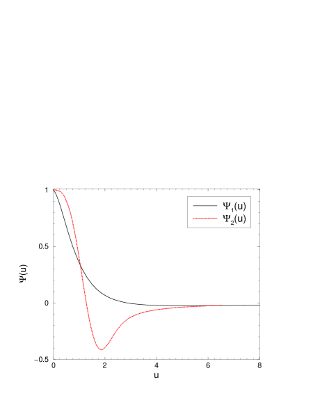
Figure 9: Scaling functions $\Psi_{1,2}(u)$ for the two-point functions $F_{i}(t,r)=t^{-2x/3}\Psi_{i}(u)$, for ${\cal M}=1$ and $\Psi_{0}=1$.

Appendix D.

We discuss the solution of the fractional-order differential equation (4.22) in terms of series expansion, following standard lines [79, 91]. As in section 4, we have $N=N_{0}+p/q$ with $N_{0}\in\mathbb{N}$. We make the ansatz

$$\Omega(v)=\sum_{n=0}^{\infty}a_{n}v^{n/q+s}\;\;,\;\;a_{0}\neq 0$$ (D1)

and from substitution into eq. (4.22), we find for $N_{0}\geq 2$,

$$\sum_{n=-p-qN_{0}}^{\infty}\frac{\alpha_{1}\Gamma\left(\frac{1}{q}(n+p+qN_{0})+s+1\right)}{\Gamma\left(\frac{n}{q}+2+s\right)}a_{n+p+qN_{0}}v^{n/q}-\sum_{n=0}^{\infty}\left(\frac{1}{q}(n+px_{1}+qN_{0}x_{1})+s\right)a_{n}v^{n/q}=0$$ (D2)

where the definition (A2) has been used. The singular terms can be dropped if $v$ is positive. Since this equation holds for all $v>0$, we obtain the following conditions. First, since $a_{0}\neq 0$, we must have

$$\frac{\alpha_{1}\Gamma\left(s+1\right)}{\Gamma\left(-\frac{p}{q}-N_{0}+2+s\right)}=0$$ (D3)

Second, we have $a_{\ell}=0$ for $\ell=1,\ldots,p+qN_{0}-1$. Finally, we get the recurrence

$$\frac{\alpha_{1}\Gamma\left(\frac{1}{q}(n+p+qN_{0})+s+1\right)}{\Gamma\left(\frac{n}{q}+2+s\right)}a_{n+p+qN_{0}}=\left(\frac{1}{q}(n+px_{1}+qN_{0}x_{1})+s\right)a_{n}$$ (D4)

From the first condition eq. (D3), we find the possible values of $s$, namely

$$s=s_{m}:=\frac{p}{q}+m\;\;,\;\;m=0,1,\ldots,N_{0}-2$$ (D5)

Negative values of $s$ would lead to a singularity as $v\to 0$ and are therefore excluded. The second and third conditions are solved by writing $n=(p+qN_{0})\ell$ and by letting $\omega_{\ell}:=a_{(p+qN_{0})\ell}=a_{n}$. We then find

$$\omega_{\ell+1}=\frac{N^{2}}{\alpha_{1}}\left(\ell+\frac{s_{m}+\zeta}{N}\right)\left(\ell+\frac{1+\zeta}{N}\right)\frac{\Gamma(N\ell+s_{m}+1)}{\Gamma(N(\ell+1)+s_{m}+1)}\,\omega_{\ell}$$ (D6)

The $N_{0}-1$ linearly independent solutions are, with $\varepsilon=N-N_{0}$

$$\Omega_{(m)}(v) = \sum_{\ell=0}^{\infty}\omega_{\ell}\,v^{N\ell+\varepsilon+m}$$ (D7)

$$= v^{\varepsilon+m}\omega_{0,m}\sum_{\ell=0}^{\infty}\frac{\Gamma(l+(s_{m}+\zeta)/N)\Gamma(l+(s_{m}+1)/N)}{\Gamma((s_{m}+\zeta)/N)\Gamma((s_{m}+1)/N)}\frac{\Gamma(s_{m}+1)}{\Gamma(N\ell+s_{m}+1)}\left(\frac{N^{2}}{\alpha_{1}}v^{N}\right)^{\ell}~{}~{}~{}~{}~{}$$

where $m=0,1,\ldots,N_{0}-2$ and $\omega_{0,m}$ are arbitrary constants. It is easy to see that these series have an infinite radius of convergence, provided $N>2$. Although this solution was only derived for rational values of $N=N_{0}+\varepsilon$, we can make the analytical continuation to all real values of $N$.

We have seen in section 4 that there are solutions of eq. (4.22) such that $\Omega(v)\sim v^{-\zeta}$ for $v$ large. These may be constructed from the series (D7) in the same way as done for $N$ integer in section 4. On the other hand, for $v$ small, one has $\Omega_{(0)}(v)\sim v^{\varepsilon}$. Therefore, the boundary condition $\Omega(0)=1$ cannot be satisfied for $\varepsilon>0$, that is any non-integer value of $N$.

This difficulty with the $v\to 0$ boundary condition is a specific property of the fractional derivative (A2) which it has in common with the Riemann-Liouville derivative. It is known that initial conditions for ordinary fractional differential equations are specified in terms of fractional derivatives $\partial^{a}f(0)$ [79, 99, 91, 60] and not in terms of ordinary derivatives $f^{(N)}(0)$ of integer order $N$. Indeed, it has been suggested to avoid this problem by using the fractional Caputo derivative instead [91, 60]. However, the Caputo derivative does not commute and it appears to be an open mathematical problem if the Caputo definition can be modified such as to obtain a commutative operator.

References

- [1] M.A. Abramowitz and I.A. Stegun, Handbook of Mathematical Functions, Dover (New York 1965)
- [2] A. Aharanoy, in C. Domb and M.S. Green (eds), Phase Transitions and Critical Phenomena, Vol. 6, Academic (London 1976), p. 358
- [3] L.C. de Albuquerque and M.M. Leite, J. Phys. A35, 1807 (2002); A34, L327 (2001).
- [4] V. Bargmann, Ann. of Math. 59, 1 (1954).
- [5] A. Barrat, Phys. Rev. E57, 3629 (1998).
- [6] A.O. Barut, Helv. Phys. Acta 46, 496 (1973).
- [7] F.S. Bates, W. Maurer, T.P. Lodge, M.F. Schulz, M.W. Matsen, K. Almdal, and K. Mortensen, Phys. Rev. Lett. 75, 4429 (1995).
- [8] A.A. Belavin, A.M. Polyakov and A.B. Zamolodchikov, Nucl. Phys. B241, 333 (1984).
- [9] J. Benzoni, J. Phys. A17, 2651 (1984).
- [10] L. Berthier, J.L. Barrat and J. Kurchan, Eur. Phys. J. B11, 635 (1999).
- [11] L. Berthier, P.C.W. Holdsworth, and M. Sellitto, J. Phys. A34, 1805 (2001).
- [12] A.J. Bray, K. Humayun and T.J. Newman, Phys. Rev. B43, 3699 (1991).
- [13] A.J. Bray, Adv. Phys. 43, 357 (1994).
- [14] A.J. Bray in [20], sect 5.4.
- [15] J.P. Bouchaud, L.F. Cugliandolo, J. Kurchan and M. Mézard, in A.P. Young (ed.) Spin Glasses and Random Fields, World Scientific (Singapore 1998); (cond-mat/9702070).
- [16] P. Calabrese and A. Gambassi, Phys. Rev. E65, 066120 (2002).
- [17] S.A. Cannas, D.A. Stariolo and F.A. Tamarit, Physica A294, 362 (2001).
- [18] J.L. Cardy, J. Phys. A18, 2771 (1985).
- [19] J.L. Cardy, Scaling and Renormalization in Statistical Mechanics Cambridge University Press, (Cambridge, 1996).
- [20] M.E. Cates and M.R. Evans (eds), Soft and Fragile Matter, Proc. 53rd Scottish University Summer Schools in Physics, (Bristol 2000).
- [21] C. Chamon, M.P. Kennett, H. Castillo and L.F. Cugliandolo, cond-mat/0109150.
- [22] B. Chopard and M. Droz, Cellular Automata Modelling of Physical Systems, Cambridge University Press (Cambridge 1998).
- [23] A. Coniglio, P. Ruggiero and M. Zanetti, Phys. Rev. E50, 1046 (1994).
- [24] F. Corberi, E. Lippiello and M. Zanetti, Phys. Rev. E65, 046136 (2002).
- [25] R. Courant and F. John, Introduction to Calculus and Analysis, Vol. I, Wiley (New York 1965), p. 566
- [26] L.F. Cugliandolo, J. Kurchan, and G. Parisi, J. Physique I4, 1641 (1994).
- [27] L.F. Cugliandolo and J. Kurchan, J. Phys. A27, 5749 (1994).
- [28] L.F. Cugliandolo and D.S. Dean, J. Phys. A28, 4213 (1995).
- [29] S. Dattagupta, Physica A194, 137 (1993).
- [30] H.W. Diehl and M. Shpot, Phys. Rev. B62, 12338 (2000).
- [31] H.W. Diehl and M. Shpot, J. Phys. A34, 9101 (2001).
- [32] H.W. Diehl and M. Shpot, J. Phys.A35, 6249 (2002).
- [33] H.W. Diehl, Acta physica slovaka 52, 271 (2002).
- [34] J.M. Drouffe et C. Itzykson, Théorie statistique des champs, 2 Vols., Editions CNRS (Paris 1988)
- [35] H.G. Evertz and D.P. Landau, Phys. Rev. B54, 12302 (1996).
- [36] H.G. Evertz and W.v.d. Linden, Phys. Rev. Lett. 86, 5164 (2001).
- [37] M.E. Fisher in F.J.W. Hahne (ed), Critical Phenomena, Springer Lecture Notes in Physics 186, Springer (Heidelberg 1983), p. 1
- [38] D.S. Fisher and D.A. Huse, Phys. Rev. B38, 373 (1988).
- [39] M. Flohr, hep-th/0111228.
- [40] L. Frachebourg and M. Henkel, Physica A195, 577 (1993).
- [41] P. di Francesco, P. Mathieu and D. Sénéchal, Conformal Field Theory, Springer (Heidelberg 1997).
- [42] I.M. Gelfand and G.E. Shilov, Generalized Functions, Vol. 1, Academic Press (New York 1964).
- [43] R.J. Glauber, J. Math. Phys. 4, 294 (1963).
- [44] J. de Gier, B. Nienhuis, P.A. Pearce and V. Rittenberg, cond-mat/0205467.
- [45] D. Giulini, Ann. of Phys. 249, 222 (1996).
- [46] C. Godrèche and J.M. Luck, J. Phys. A33, 1151 (2000).
- [47] C. Godrèche and J.M. Luck, J. Phys. A33, 9141 (2000).
- [48] C. Godrèche and J.M. Luck, J. Phys. Cond. Matt. 14, 1589 (2002).
- [49] M.D. Grynberg, T.J. Newman and R.B. Stinchcombe, Phys. Rev. E50, 957 (1994).
- [50] C.R. Hagen, Phys. Rev. D5, 377 (1972).
- [51] B.I. Halperin and P.C. Hohenberg, Rev. Mod. Phys. 49, 435 (1977).
- [52] M. Henkel, Int. J. Mod. Phys. C3, 1011 (1992).
- [53] M. Henkel, J. Stat. Phys. 75, 1023 (1994).
- [54] M. Henkel and G.M. Schütz, Int. J. Mod. Phys. B8, 3487 (1994).
- [55] M. Henkel, Phys. Rev. Lett. 78, 1940 (1997).
- [56] M. Henkel and D. Karevski, J. Phys. A31, 2503 (1998).
- [57] M. Henkel, Phase Transitions and Conformal Invariance, Springer (Heidelberg 1999).
- [58] M. Henkel, M. Pleimling, C. Godrèche and J.-M. Luck, Phys. Rev. Lett. 87, 265701 (2001).
- [59] M. Henkel and M. Pleimling, cond-mat/0108454, Comm. Comp. Phys. in press
- [60] R. Hilfer (ed), Applications of Fractional Calculus in Physics, World Scientific (Singapore 2000).
- [61] J.A. Hertz, Phys. Rev. B14, 1165 (1976).
- [62] E. Hille, Ordinary Differential Equations in the Complex Domain, Wiley (New York 1976).
- [63] H. Hinrichsen, Adv. Phys. 49, 1 (2000).
- [64] R.M. Hornreich, M. Luban and S. Shtrikman, Phys. Rev. Lett. 35, 1678 (1975).
- [65] D.A. Huse, Phys. Rev. B40, 304 (1989).
- [66] H.K. Janssen, B. Schaub and B. Schmittmann, Z. Phys. B73, 539 (1989).
- [67] D. Kandel, E. Domany and B. Nienhuis, J. Phys. A23, L755 (1990).
- [68] K. Kaski and W. Selke, Phys. Rev. B31, 3128 (1985).
- [69] M.P. Kennett and C. Chamon, Phys. Rev. Lett. 86, 1622 (2001).
- [70] M. Klimek, J. Phys. A34, 6167 (2001).
- [71] H.J. Kreuzer, Nonequilibrium Thermodynamics and its Statistical Foundation, Clarendon Press (Oxford 1981).
- [72] J. Krug, Adv. Phys. 46, 139 (1997).
- [73] J. Kurchan, cond-mat/0110628.
- [74] V.I. Lahno, J. Phys. A31, 8511 (1998).
- [75] J.-M. Levy-Leblond, Comm. Math. Phys. 4, 157 (1967); 6, 286 (1967)
- [76] E. Lippiello and M. Zanetti, Phys. Rev. E61, 3369 (2000).
- [77] J. Marro and R. Dickman, Nonequilibrium Phase Transitions in Lattice Models, Cambridge University Press (Cambridge 1999).
- [78] T. Mehen, I.W. Stewart and M.B. Wise, Phys. Lett. B474, 145 (2000).
- [79] K.S. Miller and B. Ross, An introduction to the fractional calculus and fractional differential equations, Wiley (New York 1993).
- [80] Z. Mo and M. Ferer, Phys. Rev. B43, 10890 (1991).
- [81] B. Neubert, M. Pleimling and R. Siems, Ferroelectrics 208-209, 141 (1998).
- [82] T.J. Newman and A.J. Bray, J. Phys. A23, 4491 (1990).
- [83] J.F. Nicoll, G.F. Tuthill, T.S. Chang and H.E. Stanley, Phys. Lett. A58, 1 (1976).
- [84] U. Niederer, Helv. Phys. Acta 45, 802 (1972); 46, 191 (1973); 47, 119 and 167 (1974); 51, 220 (1978).
- [85] K. Ohwada, Y. Fujii, N. Takesue, M. Isobe, Y. Ueda, N. Nakao, Y. Wakabayashi, Y. Murakami, K. Ito, Y. Amemiya, Y. Fujihisa, K. Aoki, T. Shobu, Y. Noda and N. Ikeda, Phys. Rev. Lett. 87, 086402 (2001).
- [86] J. Oitmaa, J. Phys. A18, 365 (1985).
- [87] M. Perroud, Helv. Phys. Acta 50, 233 (1977).
- [88] A. Picone and M. Henkel, J. Phys. A35, 5575 (2002).
- [89] A. Picone and M. Henkel, to be published.
- [90] M. Pleimling and M. Henkel, Phys. Rev. Lett. 87, 125702 (2001).
- [91] I. Podlubny, Fractional differential equations, Academic Press (New York 1999).
- [92] A.M. Polyakov, Sov. Phys. JETP 12, 381 (1970).
- [93] V. Privman (Ed.) Nonequilibrium Statistical Mechanics in One Dimension, Cambridge University Press (Cambridge 1996).
- [94] M.R. Rahimi Tabar, hep-th/0111327.
- [95] A.D. Rutenberg and A.J. Bray, Phys. Rev. E51, 5499 (1995).
- [96] A.D. Rutenberg, Phys. Rev. E54, R2181 (1996).
- [97] A.D. Rutenberg and B.P. Vollmayr-Lee, Phys. Rev. Lett. 83, 3772 (1999).
- [98] S. Sachdev, Quantum Phase Transitions, Cambridge University Press (Cambridge 2000).
- [99] S.G. Samko, A.A. Kilbas and O.I. Marichev, Fractional Integrals and derivatives, Gordon and Breach (Amsterdam 1993).
- [100] L. Schäfer, J. Phys. A9, 377 (1975).
- [101] G.M. Schütz and S. Sandow, Phys. Rev. E49, 2726 (1994).
- [102] G.M. Schütz, in C. Domb and J.L. Lebowitz (eds), Phase Transitions and Critical Phenomena, Vol. 19, Academic (New York 2000).
- [103] B. Schmittmann and R.K.P. Zia, in C. Domb and J.L. Lebowitz (eds), Phase Transitions and Critical Phenomena, Vol. 17, Academic (New York 1995).
- [104] A. Schröder, G. Aeppli, E. Bucher, R. Ramazashvili, and P. Coleman, Phys. Rev. Lett. 80, 5623 (1998).
- [105] W. Selke, Z. Phys. B27, 81 (1977) and Phys. Lett. A61, 443 (1977).
- [106] W. Selke, Phys. Rep. 170C, 213 (1988).
- [107] W. Selke, in C. Domb and J.L. Lebowitz (eds) Phase Transitions and Critical Phenomena, Vol.15, Academic Press (New York, 1992).
- [108] M. Shpot and H.W. Diehl, Nucl. Phys. B612, 340 (2001).
- [109] M. S̆karabot, R. Blinc, I. Mus̆evic̆, A. Rastegar, and Th. Rasing, Phys. Rev. E61, 3961 (2000).
- [110] L. Turban and F. Iglói, Phys. Rev. B66, 014440 (2002).
- [111] Y. M. Vysochanskii and V. U. Slivka, Usp. Fiz. Nauk 162, 139 (1992).
- [112] U. Wolff, Phys. Rev. Lett. 62, 361 (1989).
- [113] E.M. Wright, Proc. London Math. Soc. 46, 389 (1940); J. London Math. Soc. 27, 256 (1952) erratum.
- [114] J.M. Yeomans, Solid State Physics 41, 151 (1988).
- [115] P. Závada, Comm. Math. Phys. 192, 261 (1998).
- [116] J. Zinn-Justin, Quantum Field Theory and Critical Phenomena, Clarendon Press (Oxford 1989, 19963)
- [117] W. Zippold, R. Kühn and H. Horner, Eur. Phys. J. B13, 531 (2000).
- [118] P. Calabrese and A. Gambassi, cond-mat/0207487.