hep-th/0205162

EFI-02-71

LPTENS-02/27, PAR-LPTHE 02-26

Twisting $E8$ Five-Branes

Arjan Keurentjes^a and Savdeep Sethi^b

^a LPTHE, Université Pierre et Marie Curie, Paris VI, Tour 16,
4 place Jussieu, F-75252 Paris Cedex 05, France
and
Laboratoire de Physique Théorique de l’Ecole Normale Supérieure,
24 rue Lhomond, F-75231 Paris Cedex 05, France
^b Enrico Fermi Institute, University of Chicago, Chicago, IL 60637, USA
and
School of Natural Sciences, Institute for Advanced Study, Princeton, NJ 08540

We consider the tensor theory on coincident $E8$ $5$-branes compactified on $T^{3}$. Using string theory, we predict that there must be distinct components in the moduli space of this theory. We argue that new superconformal field theories are to be found in these sectors with, for example, global $G_{2}$ and $F_{4}$ symmetries. In some cases, twisted $E8$ $5$-branes can be identified with small instantons in non-simply-laced gauge groups. This allows us to determine the Higgs branch for the fixed point theory.

We determine the Coulomb branch by using an M theory dual description involving partially frozen singularities. Along the way, we show that a D0-brane binds to two D4-branes, but not to an $Sp$-type O4-plane (despite the existence of a Higgs branch). These results are used to check various string/string dualities for which, in one case (quadruple versus NVS), we present a new argument. Finally, we describe the construction of new non-BPS branes as domain walls in various heterotic/type I string theories.

1 Introduction

The $5$-brane of the $E_{8}\times E_{8}$ heterotic string can be viewed as the small size limit of an $E_{8}$ instanton [2, 3]. Supported on the $5$-brane is a $(1,0)$ tensor theory which is both mysterious and fascinating. From its origin as the zero size limit of an instanton, we know that the theory has a Higgs branch parametrized by $29$ massless hypermultiplets. This branch describes the $E_{8}$ instanton together with its moduli. There is also a Coulomb branch parametrized by the single scalar of a $(1,0)$ tensor multiplet. The expectation value of the scalar determines the position of the $5$-brane in the M theory direction. At the intersection of these two branches is a superconformal field theory with $8$ supercharges, and global $E_{8}$ symmetry. For $N$ $5$-branes, the structure is similar. The Higgs branch has $30N-1$ light hypermultiplets, while the Coulomb branch has $N$ light tensor multiplets.

While little is known about interacting tensor theories, it is conventional wisdom that when compactified on a torus, these theories reduce to Yang-Mills theories. Compactifications of small instanton theories have been studied in [4, 5, 6]. One of the interesting properties of Yang-Mills theory, first discussed in [7] for the case of $SU(N)/{\mathbb{Z}}_{N}$, is the possibility of turning on ‘non-abelian magnetic flux’ on a $2$-cycle. More generally, for gauge group $G/Z(G)$ where $G$ has center $Z(G)$, the magnetic flux on a space ${\cal M}$ is classified by $H^{2}({\cal M},Z(G))$.

We might then imagine that the choice of flux on $T^{3}$ can be studied by first reducing to gauge theory on one circle, and then studying the possible ’t Hooft twists in this gauge theory. Using string theory, we shall see that this is not true for the $E_{8}$ $5$-brane: there are new sectors on $T^{3}$ with no corresponding gauge theory interpretation. These sectors are distinguished by a kind of tensor flux analogue of magnetic flux. This is fairly basic property of these interacting $(1,0)$ theories that we might hope to understand from first principles.

The effective $2+1$-dimensional physics in these exotic sectors includes interacting superconformal field theories with $16$ superconformal charges, and various exotic global symmetries (listed in table 1). To each of these new fixed points labeled by the number of branes $N$, there should correspond an $AdS_{4}$ gauged supergravity with $16$ supersymmetries. Establishing the existence of these theories would provide a beautiful link between the classification of flat bundles in gauge theory – in this case, triples of commuting connections – and gauged supergravities.

We determine the Higgs and Coulomb branches for these fixed point theories in the following way: the structure of the Higgs branch follows from viewing these branes as small instantons in non-simply-laced gauge groups. These instantons can be studied by probing various orientifold $4$-planes with D0-branes. In this way, we resolve some puzzles in the ADHM construction for orthogonal groups. We also show that in the case of a pure $\mathrm{O}4^{+}$-plane which supports no space-time gauge group (but with D4-branes supports an $Sp$ group), there are still localized “$Sp(0)$” instantons. Nevertheless, using $L^{2}$ index theory and the theorem of [8], we show that a bulk D0-brane does not bind to an $\mathrm{O}4^{+}$-plane even though there is a Higgs branch. It does, however, bind in a unique way to $2$ D4-branes. Since a D0-brane binds uniquely to $1$ D4-brane [9], it seems highly likely that it binds uniquely to any number of D4-branes. These results agree with the analysis of [10, 11], where the bulk term for $1$ D0-brane with $2$ D4-branes is computed. Our result for $2$ D4-branes also agrees with expectations from a moduli space analysis [12]. Determining the index and the bulk terms for arbitrary numbers of D0 and D4-branes remains an outstanding question. It might be possible to compute the bulk terms using [13, 14]. To determine the Coulomb branch, we use a duality between triple compactifications, and $K3$ surfaces with frozen singularities [15].

We proceed by applying our binding results to the question of string/string duality. In the familiar duality between heterotic on $T^{4}$ and IIA on $K3$, the IIA string is constructed using a heterotic $5$-brane wrapping $T^{4}$. We extend this construction to the case of the CHL string on $T^{4}$ versus IIA on a $K3$ with $8$ frozen $A_{1}$ singularities [16]. We show that the light spectrum for the wrapped $5$-brane agrees with our expectations for a IIA string on a partially frozen $K3$ surface. We also provide a new argument for the equivalence of two type I compactifications: one with a quadruple gauge bundle, and one with a no vector structure (NVS) compactification. In this approach, the duality becomes completely geometric.

Our final topic is the construction of domain walls bridging disconnected string vacua. These vacua each have zero cosmological constant, and there must exist a field theoretic instanton that tunnels from one to the other. In Yang-Mills, this instanton should be BPS carrying fractional charge. What is particularly nice about this setup is that the vacua are quite simple. Also, the tunneling involves no change in topology, and so occurs at finite energy.

When embedded in gravity, there are two modifications: first, we need to use an instanton/anti-instanton pair to tunnel so the configuration becomes non-BPS (but stable). We also expect it to become time-dependent, with a metric on the wall that looks like a slice of deSitter space in the thin wall approximation [18]. Finding CFT/supergravity solutions for these domain walls would allow us to go beyond string theory in a fixed background, and perhaps shed light on questions of cosmology. For prior work on domain walls in the heterotic string, see [19]. While our discussion is confined primarily to $E_{8}$ $5$-branes wrapped on $T^{3}$, similar phenomena occur for type I D5-branes on $T^{4}$, and Euclidean D5-branes on $T^{6}$ where there are new components in the string moduli space [20, 21]. We conclude with a brief comment on the domain walls we expect in those cases.

2 Small Instantons in Non-simply-laced Groups

2.1 The normalization of instanton charges

We begin our discussion of instantons by recalling an old theorem by Bott [23]. It states that any continuous mapping of $S^{3}$ into a group $G$ can be continuously deformed into a mapping of $S^{3}$ into an $SU(2)$ subgroup of $G$. Therefore, as far as instantons are concerned, we need only study $SU(2)$ subgroups. We will study the instantons in string theory at loci in the moduli space where there is enhanced gauge symmetry. Close to such a locus, any scalars in a vector multiplet act as Higgs fields in the adjoint representation of $G$. Breaking the gauge symmetry with adjoint Higgs fields can only result in special subgroups of $G$, which are called regular subgroups. A regular subgroup has a root lattice which is a sublattice of the full root lattice of the group $G$. An adjoint Higgs can be transformed (locally, by a gauge transformation) into an element of the Cartan subalgebra. It is then easy to see that the group left unbroken is the one that commutes with this element, and that it must be regular. There exists an elegant method due to Dynkin for determining all regular subgroups of a given group [24]. However, we will only be interested in $SU(2)$ subgroups, which can easily be found by inspection. From these preliminaries, we conclude that we should study instantons of regular $SU(2)$ subgroups of $G$.

After deformation to an $SU(2)$ subgroup, the instanton charge is given by,

$$\frac{1}{8\pi^{2}N_{R}}\int~{}\textrm{Tr}\,(F\wedge F)=\frac{2\textrm{Tr}(T^{a}T^{b})}{16\pi^{2}N_{R}}\int_{{\mathbb{R}}^{4}}\textrm{d}^{4}x~{}{}^{*}\!F^{a}_{\mu\nu}F^{b\mu\nu}.$$ (1)

The constant $N_{R}$ is a normalization factor which depends on which representation, $R$, of the group, $G$, we consider. It is inserted to normalize the smallest possible instanton charge to 1. For example, if $R$ is the adjoint representation, then $N_{R}$ is twice the dual Coxeter number. On the right hand side, we have extracted the generators $T^{a}$ for the $SU(2)$ subgroup from the expression. The integral can now be evaluated for an arbitrary $n$-instanton solution. It is crucial that the charge is multiplied by $2\textrm{Tr}(T^{a}T^{b})$ (the factor of 2 ensures that this is integer). One can equate this factor to $k\delta^{ab}$, with $k$ an integer, known as the embedding or Dynkin index [24] (see also [25, 26] for related material).

In string theory, where gauge symmetries originate from current algebra, the integer $k$ is the level of the current algebra in the current algebra and is called the level. In the operator product of two currents, $J^{a}$, the level is the coefficient of the Schwinger term:

$$J^{a}(z)J^{b}(w)=\frac{k\delta^{ab}}{(z-w)^{2}}+\ldots.$$ (2)

For a nice review of the implications of the Kac-Moody level in string theory, see [27].

To compute the Dynkin index is not hard: the index for a reducible $SU(2)$ representation is the sum of the indices of all its irreducible factors. Let the irreducible representations of $SU(2)$ be labeled by their dimension $d$, then

$$k=\frac{d(d^{2}-1)}{6}$$ (3)

as can be verified by using the eigenvalues of $\sigma^{3}$ in the appropriate irrep.

Let us consider a relevant example. The smallest non-simply-laced group is $SO(5)\cong Sp(2)$. This group has inequivalent regular $SU(2)$ subgroups. To find the first one, we decompose

$$SO(5)\rightarrow SO(4)\cong SU(2)\times SU(2)$$

and choose one of the $SU(2)$ factors. The $\mathbf{4}$, $\mathbf{5}$ and $\mathbf{10}$ (the spin, vector, and adjoint irreps of $SO(5)$) decompose in the following way,

$$\mathbf{4}\rightarrow\mathbf{2\oplus 1\oplus 1}\qquad\mathbf{5}\rightarrow\mathbf{2\oplus 2\oplus 1}\qquad\mathbf{10}\rightarrow\mathbf{3\oplus 2\oplus 2\oplus 1\oplus 1\oplus,1}$$ (4)

and so we find that $k=1,2,6$, respectively. A charge 1 instanton embedded in this $SU(2)$ subgroup has the smallest charge possible, and indeed one should set $N_{\bf 4}=1,N_{\bf 5}=2$ and $N_{\bf 10}=6$.

A second $SU(2)$ subgroup can be found by decomposing

$$SO(5)\rightarrow SO(3)\times SO(2).$$

We now embed the instanton in the $SO(3)$ factor. In this case, the decompositions are given by

$$\mathbf{4}\rightarrow\mathbf{2\oplus 2}\qquad\mathbf{5}\rightarrow\mathbf{3\oplus 1\oplus 1}\qquad\mathbf{10}\rightarrow\mathbf{3\oplus 3\oplus 3\oplus 1}.$$ (5)

This gives $k=2,4,12$, respectively. The instanton charge in this case is twice as large as in the previous example. It is not hard to see that if $SO(5)$ is broken with only adjoint Higgs fields, only the second breaking is possible. Therefore, any breaking of $SO(5)$ by adjoint Higgs fields can preserve, at most, instanton configurations with even charge.

The previous discussion can be rephrased in a slightly more abstract way in terms of properties of the group lattice of the non-simply-laced group. This will allow us to generalize to the case of a semi-simple gauge group with factors at different levels. In either case, by definition, there are roots of different lengths. We can focus on the case where there are two different lengths, with the generalization clear. By standard group theory, we can associate an $SU(2)$ subgroup to every root, and these are the groups in which we will embed elementary instantons.

Any two $SU(2)$ subgroups corresponding to roots of different lengths clearly cannot be conjugate. Hence their instanton solutions are in general also inequivalent, no matter where we are in the moduli space. The various representations of $G$ are generated by vectors in the weight lattice. The lattice dual to the weight lattice, known as the coroot lattice, determines the global structure of any subgroup that we might choose to study. The periodicity of any generator for an $su(2)$ subalgebra can be determined from the coroot lattice.

A long root corresponds to a short coroot, and vice versa. Suppose one has a root with length $p$, and another root with length $q$. The same instanton solution, embedded in either of the $SU(2)$ subgroups associated to these roots, will result in inequivalent solutions whose charges have a ratio $q/p$. The solution of smallest charge occurs in the subgroup associated to the largest root (and therefore the smallest coroot). In the above $SO(5)$ example, it is not hard to verify that the two different solutions correspond to decompositions which use either a long or a short root of the $SO(5)$ algebra, respectively.

Note that the multiplicative normalization of the instanton charge is proportional to the level, but inversely proportional to the lengths of the roots of the various subgroups. We can now embark on a study of instantons in string theories where non-simply-laced groups, and groups at different levels appear.

2.2 Instantons and orientifolds

Much of what we have just described can be understood more intuitively using orientifolds. We use the conventions of [15] where an $\mathrm{O}p^{+}$-plane together with $N$ D$p$-branes supports an $Sp(N)$ gauge group. An $\mathrm{O}p^{-}$-plane with $N$ D$p$-branes supports an $SO(2N)$ group, while $\widetilde{\mathrm{O}p}{}^{-}$ supports an $SO(2N+1)$ gauge group.

Consider $\mathrm{O}4^{+}$ with $N$ pairs of coincident D4-branes. The orientifold plane supports an $Sp(N)$ gauge group, which is non-simply-laced. Instantons in this gauge theory can be realized by D0-branes which are stuck to the orientifold plane. It is natural for us to ask about the dynamics of D0-brane probes of the orientifold plane. The quantum mechanical gauge theory on $k$ D0-brane probes of $O4^{+}$ has $8$ real supercharges. It has gauge group $O(k)$ with a hypermultiplet transforming as a rank $2$ symmetric tensor. The global symmetry of the theory is $Sp(N)$, and the D0-D4 strings give a half-hypermultiplet transforming in the bifundamental of $O(k)\times Sp(N)$. The Higgs branch of the theory is the moduli space of $k$ $Sp(N)$ instantons. The case $k=1$ corresponds to a ${\mathbb{Z}}_{2}$ gauge group. A single D0-brane can be stuck at the location of the orientifold plane, and cannot move into the bulk. Therefore, there is no Coulomb branch. This is true for any choice of $N$, including $N=0$. In this case, the D0-branes correspond to “Sp(0)” instantons.

Figure 1: $Sp(N)$: the long root should be identified with the orientifold plane.

That a single D0-brane can localize at an $\mathrm{O}4^{+}$-plane can also be understood by interpreting the D0-branes as small instantons in the D4 gauge theory. Since $Sp(N)$ is non-simply-laced, it has roots of different length. We can move pairs of D4-branes away from the orientifold plane, but the group at the $\mathrm{O}4^{+}$ remains symplectic. A comparison with the Dynkin diagram of $Sp(N)$ suggests that we should associate the long root of the Dynkin diagram with the $\mathrm{O}4^{+}$-plane. For a similar observation, see [31]. What is important for us is the periodicity of the group, which is determined by the coroots. The long roots of $Sp(N)$ give rise to short coroots. Instantons with the smallest possible charge have to be embedded in the $SU(2)$ associated with the short coroots. To these instantons, we assign charge one. By contrast, it is natural to assign charge two to instantons living in the $U(N)$ theory on bulk D4-branes separated from the $\mathrm{O}4^{+}$-plane. If there were no $\mathrm{O}p^{+}$-plane, these instantons would have the smallest charge possible, and it would then be natural to assign them charge one.

2.3 Can a D0-brane stick to an $\mathrm{O}4^{+}$-plane?

2.3.1 Symmetries and supercharges

Let us take $k=2$ with $N=0$. This particular case will play a role in later discussion. The D0-brane gauge theory now has a Coulomb branch, and so the probe can move in the bulk. Although there is no gauge group localized at the orientifold plane, the D0-brane might still bind to the orientifold plane. To address this question, we use $L^{2}$ index theory.

In addition to an $O(2)$ vector multiplet, there is one hypermultiplet transforming as a second rank symmetric tensor; see, for example, [32]. We can factor out the trace, which gives a decoupled hypermultiplet. This hypermultiplet parametrizes the position of the D0-brane along the $\mathrm{O}4^{+}$-plane. What remains are $2$ hypermultiplets with charge $2$ under the $SO(2)$ subgroup of $O(2)$. We anticipate however that in the computations below, the charge will not make any difference. We will therefore denote it by $e_{0}$, and demonstrate explicitly that our end result does not depend on this variable. The symmetry group for $2$ hypermultiplets is $Sp(2)_{L}\times Sp(1)_{R}$. We realize the R-symmetry via the $Sp(1)_{R}$ action. The gauge symmetry commutes with the R-symmetry, and so must sit in $Sp(2)_{L}$. Note that a single hypermultiplet is not possible in this case because $O(2)$, unlike $SO(2)$, cannot be faithfully embedded in $Sp(1)_{L}$. However, we can embed $O(2)$ into $Sp(2)_{L}$. The full symmetry group of the theory is the combination of the dimensionally reduced Lorentz group and the R-symmetry, $Spin(5)\times Sp(1)_{R}$. Our conventions follow those of [33].

The vector multiplet contains $5$ scalars, $X^{\mu}$, which are in the $(\bf{5},\bf{1})$ of the symmetry group. These scalars are inverted by the $O(2)$ group element,

$$g_{\rm o}=\pmatrix{1&0\cr 0&-1},$$ (6)

but uncharged under the $SO(2)$ subgroup. Let $P^{\mu}$ be the associated canonical momenta obeying,

$${\left[X^{\mu},P^{\nu}\right]}=i\delta^{\mu\nu}.$$ (7)

The superpartners of these bosons are eight real fermions, $\lambda_{a}$, where $a=1,\ldots,8$ transforming in the $(\bf{4},\bf{2})$ representation. These fermions obey the usual quantization relation,

$${\left\{\lambda_{a},\lambda_{b}\right\}}=\delta_{ab}.$$ (8)

We also need hermitian real gamma matrices, $\gamma^{\mu}$, which obey

$${\left\{\gamma^{\mu},\gamma^{\nu}\right\}}=2\delta^{\mu\nu}.$$ (9)

To complete the vector multiplet, we introduce an auxiliary field, $D$, which transforms as $({\bf 1},{\bf 3})$ under the symmetry group. Supersymmetry requires that it be an imaginary quaternion, independent of $X^{\mu}$. The vector multiplet supercharge is given by:

$$Q^{v}=\not\!\!P\lambda+\frac{e_{0}}{2}D\lambda.$$ (10)

A hypermultiplet contains four real scalars which we can package into a quaternion $q$ with components $q^{i}$ where $i=1,2,3,4$. This field transforms as $({\bf 1},{\bf 2})$ under the symmetry group. We again introduce canonical momenta $p_{i}$ satisfying the usual commutation relations.

We have $2$ hypermultiplets, $q$ and $\widetilde{q}$ which have charge $e_{0}$ and charge $-e_{0}$, respectively, under the $U(1)$ subgroup of $O(2)$. We generate gauge transformations on the bosons (packaged into two quaternions) using left multiplication by,

$$\pmatrix{q\cr\widetilde{q}}\rightarrow I\pmatrix{0&-\bf{1}\cr\bf{1}&0}\pmatrix{q\cr\widetilde{q}}.$$

This action is realized by the operator,

$$G_{B}=\frac{1}{2}\left(\widetilde{q}\bar{p}+p\bar{\widetilde{q}}-q\bar{\widetilde{p}}-\widetilde{p}\bar{q}\right),$$ (11)

which is real as a quaternion, and therefore hermitian with respect to the components of the quaternion.

To go from $U(1)$ to $O(2)$, we will also need to gauge the ${\mathbb{Z}}_{2}$ symmetry corresponding (in a complex basis) to charge conjugation. We will return to this point momentarily. The superpartner to $(q,\widetilde{q})$ is a real fermion $(\psi_{a},\widetilde{\psi}_{a})$ with $a=1,\ldots,8$ satisfying,

$${\left\{\psi_{a},\psi_{b}\right\}}=\delta_{ab},\quad{\left\{\widetilde{\psi}_{a},\widetilde{\psi}_{b}\right\}}=\delta_{ab},\quad{\left\{\psi_{a},\widetilde{\psi}_{b}\right\}}=0$$ (12)

and transforming in the $({\bf 4},{\bf 1})$ representation. Converting the $p_{i}$ to quaternions, with the aid of the $s^{j}$ operators given in Appendix A, the free hypermultiplet charge takes the form

$$Q^{h_{f}}=p\psi+\widetilde{p}\widetilde{\psi}.$$ (13)

This free charge obeys the algebra,

$${\left\{Q^{h_{f}}_{a},Q^{h_{f}}_{b}\right\}}=\delta_{ab}(|p|^{2}+|\widetilde{p}|^{2}).$$

Invariance of $(\ref{freehyper})$ under the $U(1)$ gauge symmetry requires that

$$G_{F}=i\,(\widetilde{\psi}_{a}\psi_{a})$$ (14)

generate gauge transformations on $\psi,\widetilde{\psi}$. The total generator of the $U(1)$ subgroup of the gauge symmetry is then,

$$G=G_{B}+G_{F}=\frac{1}{2}\left(\widetilde{q}\bar{p}+p\bar{\widetilde{q}}-q\bar{\widetilde{p}}-\widetilde{p}\bar{q}\right)+i\widetilde{\psi}\psi.$$ (15)

The full hypermultiplet supercharge $Q^{h}$ also includes couplings to the vector multiplet,

$$Q^{h}=p\psi+\widetilde{p}\widetilde{\psi}+\frac{e_{0}}{2}\not\!\!X(q\widetilde{\psi}-\widetilde{q}\psi).$$ (16)

Note that the order of multiplication matters because $p,\not\!\!X,q$ are matrix-valued fields. The form of the interaction term in $(\ref{hypercharge})$ is fixed up to an overall constant by symmetry. The charge obeys the algebra:

$${\left\{Q^{h}_{a},Q^{h}_{b}\right\}}=\delta_{ab}\left\{|p|^{2}+|\widetilde{p}|^{2}+\frac{e_{0}^{2}}{4}|X|^{2}(|q|^{2}+|\widetilde{q}|^{2})-ie_{0}\,(\psi\!\not\!\!X\widetilde{\psi})\right\}+\frac{e_{0}}{2}(\not\!\!X)_{ab}G.$$ (17)

Closure of the supersymmetry algebra is, as usual, only up to gauge transformations.

The full supercharge $Q$ is the given by,

$$Q=Q^{v}+Q^{h},$$ (18)

where we define the $D$-term in the following way:

$$D=\frac{1}{2}(q\bar{\widetilde{q}}-\widetilde{q}\bar{q}).$$ (19)

The full charge obeys the algebra:

$${\left\{Q_{a},Q_{b}\right\}}=2\delta_{ab}(H_{B}+H_{F}+V)+\frac{e_{0}}{2}\not\!\!X_{ab}G$$ (20)

with

$$H_{B} =\frac{1}{2}\left(P^{2}+|p|^{2}+|\widetilde{p}|^{2}\right),$$ (21)

$$H_{F} =i\frac{e_{0}}{2}\left(\lambda\widetilde{q}\psi-\lambda q\widetilde{\psi}-\psi\!\not\!\!X\widetilde{\psi}\right),$$ (22)

$$V =\frac{e_{0}^{2}}{8}\left(|X|^{2}\{|q|^{2}+|\widetilde{q}|^{2}\}+|D|^{2}\right).$$ (23)

Lastly, we need to check that the supercharges are $O(2)$ rather than $SO(2)$ invariant. Any element of $Sp(2)_{L}$ must preserve the norm,

$$N(q,\widetilde{q})=q\bar{q}+\widetilde{q}\bar{(\widetilde{q})}.$$

Consider the element

$$\pmatrix{\bf{1}&0\cr 0&-\bf{1}}$$

which squares to one. This group element is trivially identified with the generator, $g_{o}$, given in $(\ref{go})$. Under its action,

$$(q,\psi)\leftrightarrow(q,\psi)\quad(\widetilde{q},\widetilde{\psi})\leftrightarrow(-\widetilde{q},-\widetilde{\psi}),\quad X\rightarrow-X,\quad\lambda\rightarrow-\lambda.$$ (24)

It is easy to see that $D\rightarrow-D$ so the vector multiplet charge is invariant. It is also easy to see that the hypermultiplet charge is invariant so this is a symmetry of the theory which we can gauge.

Finally we note that the centralizer of $O(2)$ inside $Sp(2)$ are matrices of the form

$$\pmatrix{S&0\cr 0&S}$$

with $S$ an element of $Sp(1)$. This diagonal $Sp(1)_{f}$ flavour symmetry, acting from the left, can be combined with the $R$ symmetry $Sp(1)_{R}$ that acts from the right. Together they give an $SO(4)$ symmetry under which the $4$ components $(q_{i},\widetilde{q}_{i})$ of each quaternion transform as a vector.

This theory has two branches. The Coulomb branch is parametrized by the $X^{\mu}$, and is ${\mathbb{R}}^{5}/{\mathbb{Z}}_{2}$. At a generic point, the discrete ${\mathbb{Z}}_{2}$ symmetry is broken, and the gauge group $SO(2)$. The Higgs branch is obtained by setting $\widetilde{q}=0,\,X=0$ (or equivalently by an $SO(2)$ gauge transformation, $q=X=0$), and quotienting by the residual ${\mathbb{Z}}_{2}$ gauge symmetry, giving ${\mathbb{R}}^{4}/{\mathbb{Z}}_{2}$. On this branch it is the $SO(2)$ symmetry which is broken to ${\mathbb{Z}}_{2}$. This leaves a residual $O(1)\times O(1)={\mathbb{Z}}_{2}\times{\mathbb{Z}}_{2}$ gauge symmetry. No FI term is possible in this theory because any allowed $D$-term must be odd under $g_{o}$. A constant $D$-term is therefore ruled out.

The Coulomb branch parametrizes motion of the D0-brane away from the orientifold plane. The Higgs branch occurs because at the $\mathrm{O}4^{+}$-plane, half-integer charged D0-branes are possible. The Higgs branch corresponds to the splitting of a bulk $\mathrm{D}0$-brane into two such half $\mathrm{D}0$-branes. The expectation value of the scalars in the hypermultiplet corresponds to the separation of the two fractionally charged constituents along the $\mathrm{O}4^{+}$-plane. There is also a decoupled hypermultiplet that describes the center of mass motion along the $\mathrm{O}4^{+}$-plane. Note that the residual gauge symmetry on the Higgs branch is exactly what we expect for two D0-branes of charge one-half.

2.3.2 The bulk term contribution

To compute the $L^{2}$ index, we need to evaluate the low-temperature limit of the twisted partition function

$${\rm Ind}=\lim_{\beta\rightarrow\infty}{\rm Tr}(-1)^{F}e^{-\beta H}.$$ (25)

This is a topic that has been analyzed in some detail, and we will use and extend the methods developed in [9, 34, 35].

We begin by computing the bulk term contribution which is the high temperature limit of the twisted partition function:

$$I(0)=\lim_{\beta\rightarrow 0}{\rm Tr}(-1)^{F}e^{-\beta H}.$$ (26)

The ${\mathbb{Z}}_{2}$ charge measuring fermion number is given by

$$(-1)^{F}=2^{12}\prod_{a=1}^{8}\lambda_{a}\prod_{a=1}^{8}\psi_{a}\prod_{a=1}^{8}\widetilde{\psi}_{a}.$$ (27)

We need to approximate the heat kernel $e^{-\beta H}$, but fortunately, the simplest approximation will suffice:

$$e^{-\beta H}(X,(q,\widetilde{q});X^{\prime},(q^{\prime},\widetilde{q}^{\prime}))={1\over(2\pi\beta)^{13/2}}\,e^{\,-{1\over 2\beta}\left(|X-X^{\prime}|^{2}+|q-q^{\prime}|^{2}+|\widetilde{q}-\widetilde{q}^{\prime}|^{2}\right)}e^{-\beta V}e^{-\beta H_{F}}(1+O(\beta)).$$ (28)

We have lumped all the bosonic potential terms into $V$. We also need to be sure that we compute the trace on gauge invariant states so we insert a projection operator into the trace,

$$I(0)=\lim_{\beta\rightarrow 0}\,\int_{-\pi}^{\pi}{d\theta\over 2\pi}\,{\rm Tr}(-1)^{F}{1\over 2}(1+\Pi(g_{o}))e^{ie_{0}\theta G_{F}}e^{-\beta H}(X,(q,\widetilde{q});X,g_{e_{0}\theta}(q,\widetilde{q})),$$ (29)

where

$$g_{e_{0}\theta}(q,\widetilde{q})=(\cos e_{0}\theta\ q-\sin e_{0}\theta\ \widetilde{q},\,\sin e_{0}\theta\ q+\cos e_{0}\theta\ \widetilde{q})$$

The projection onto $O(2)$ invariant states is performed by the insertion of, ${1\over 2}(1+\Pi(g_{o}))$, where $\Pi(g_{o})$ implements the action of $g_{o}$ on all the fields.

There are two contributions to the bulk term $(\ref{bulk})$, one with $\Pi(g_{o})$ inserted, and one without. Let us first deal with the case where $\Pi(g_{o})$ is inserted. Note that $\Pi(g_{o})$ sends $X\rightarrow-X$, and so leaves us with an approximate heat kernel,

$$e^{-\beta H}\sim\left({1\over\beta}\right)^{13/2}e^{-{2\over\beta}|X|^{2}}e^{\,-{1\over 2\beta}\left(|q-g(\theta)(q)|^{2}+|\widetilde{q}-g(\theta)(\widetilde{q})|^{2}\right)}e^{-{{\beta e_{0}^{2}}\over 8}\left(|X|^{2}(|q|^{2}+|\widetilde{q}|^{2})+|D|^{2}\right)}e^{\left(ie_{0}\theta G_{F}-\beta H_{F}\right)}.$$

We need to saturate the trace with fermions from the propagator. Otherwise, the insertion of $(-1)^{F}$ kills the trace. From the perspective of the Euclidean path-integral, inserting $(-1)^{F}$ means that the fermions have periodic boundary conditions in the time direction. Consequently, there are fermion zero-modes. Since $\Pi(g_{o})$ also sends

$$\lambda\rightarrow-\lambda,\quad\widetilde{\psi}\leftrightarrow-\widetilde{\psi},$$

there are no $\lambda$ or $\widetilde{\psi}$ zero modes, but there are $8$ $\psi$ zero modes. We now need to count powers of $\beta$. To prevent the integral from vanishing, we need to rescale $x\rightarrow{x\over\sqrt{\beta}}$ which introduces a factor of $\beta^{5/2}.$ We also rescale $\theta\rightarrow{\theta\over\sqrt{\beta}}$ which introduces $\beta^{1/2}$. Finally, we need to rescale the combination $\widetilde{q}\rightarrow{\widetilde{q}\over\sqrt{\beta}}$ which gives $\beta^{4/2}$. Schematically, what remains takes the form

$$\left({1\over\beta}\right)^{3/2}e^{-\beta^{1/2}\theta\Psi\Psi-\beta^{3/2}X\Psi\Psi-\beta q\Psi\lambda+\beta^{3/2}\widetilde{q}\Psi\lambda}$$

where $\Psi$ denotes both $\psi,\widetilde{\psi}$. To saturate the $\psi$ zero modes requires at least $4$ insertions of a $\Psi\Psi$ term. This brings down a minimum of $\beta^{2}$, which kills this contribution.

We therefore need only consider the bulk term without any $\Pi(g_{o})$ insertion. The bulk term for this $U(1)$ gauge theory only differs by a factor of $2$ from the computation for $O(2)$,

$$I(0)_{U(1)}=2I(0)_{O(2)}.$$

In the limit $\beta\rightarrow 0$, we can localize $g(\theta)$ around the identity, and make the replacement

$$e^{\,-{1\over 2\beta}\left(|q-g(\theta)(q)|^{2}+|\widetilde{q}-g(\theta)(\widetilde{q})|^{2}\right)}\quad\rightarrow\quad e^{\,-{e_{0}^{2}\theta^{2}\over 2\beta}\left(|q|^{2}+|\widetilde{q}|^{2}\right)}.$$ (30)

At this point, we examine the charge dependence of the index computation. The relevant part of the heat kernel has the form,

$$\int_{-\pi}^{\pi}\,{d\theta\over 2\pi}\,e^{-|Q-e^{ie_{0}\theta}Q|^{2}}\times\ldots,$$

where $Q$ represents the matter fields. There is a non-zero contribution from a neighborhood of each solution of

$$e^{ie_{0}\theta}=1.$$

There is only one special case which occurs when the boundary points, $\theta=\pm\pi$, are solutions. These points together give the same contribution as an interior point, $\theta\in(-\pi,\pi)$. The total contribution is then $|e_{0}|$ times larger than the case of matter with charge one.

With these comments in mind, we note that the rescaled gauge parameter, $\tilde{\theta}=\theta/\beta$, then effectively behaves like the $A_{0}$ component of the gauge-field in Euclidean space. Upon changing variables from $\theta$ to $\tilde{\theta}$, we get an additional factor of $\beta$ in the measure of our integral. From the proceeding discussion, we know that we can account for the charge dependence by simply multiplying the $\theta=0$ contribution by $e_{0}$.

In the $\beta\rightarrow 0$ limit, the range of $\tilde{\theta}$ diverges, and we can really treat $\tilde{\theta}$ on equal footing with $X^{\mu}$. If we express the fermion bilinear appearing in $\beta H_{F}-ie_{0}\theta G_{F}$ in the form $\Psi M\Psi$, where $\Psi$ collectively denotes $\lambda,\psi,\widetilde{\psi}$ then $M$ is a matrix linear in the bosons. It takes the form,

$$\frac{ie_{0}\beta}{4}\pmatrix{\lambda&\psi&\widetilde{\psi}}\pmatrix{0&\widetilde{q}&-q\cr-\widetilde{q}^{T}&0&-\not\!\!X-i\tilde{\theta}\cr q^{T}&\not\!\!X+i\tilde{\theta}&0}\pmatrix{\lambda\cr\psi\cr\widetilde{\psi}}.$$

Our task is to determine the Pfaffian. It is $SO(6)$ invariant with $(X^{\mu},\tilde{\theta})$ forming a vector $Y$ under the $SO(6)$. The Pfaffian can therefore only depend on $|Y|=\sqrt{X^{2}+\tilde{\theta}^{2}}$. To find the scaling behaviour with respect to various contributions, we use the following trick.

Multiply the first and second (quaternionic) row with a positive real number, $\rho$, and the third row with $\rho^{-1}$. Then multiply the first and second column with $\rho$, and the third with $\rho^{-1}$. The net effect of these manipulations is

$$Y\rightarrow Y,\quad q\rightarrow q,\quad\widetilde{q}\rightarrow\rho^{2}\widetilde{q},\qquad{\rm Pf}(M)\rightarrow\rho^{8}{\rm Pf}(M).$$

From this we deduce that the Pfaffian must contain 4 powers of $\widetilde{q}$. Repeating these manipulations with different combinations of rows and columns, one also finds that the Pfaffian contains $4$ powers of $q$, and $4$ of $|Y|$.

To find the Pfaffian, we make use of symmetry. First we use the $SO(6)$ symmetry to rotate to coordinates where $X^{\mu}=0$ and $\tilde{\theta}=|Y|$. Next we make use of the $Sp(1)_{f}\times Sp(1)_{R}=SO(4)$ which acts on the quaternions $q$ and $\widetilde{q}$. First act with the orthogonal matrix:

$$|q|^{-1}\pmatrix{q_{1}&q_{2}&q_{3}&q_{4}\cr-q_{2}&q_{1}&-q_{4}&q_{3}\cr-q_{3}&q_{4}&q_{1}&-q_{2}\cr-q_{4}&-q_{3}&q_{2}&q_{1}}\pmatrix{q_{1}&\widetilde{q}_{1}\cr q_{2}&\widetilde{q}_{2}\cr q_{3}&\widetilde{q}_{3}\cr q_{4}&\widetilde{q}_{4}}=|q|^{-1}\pmatrix{|q|^{2}&q_{i}\widetilde{q}_{i}\cr 0&-D_{1}\cr 0&-D_{2}\cr 0&-D_{3}}.$$

Note that this matrix effectively implements right multiplication by $\bar{q}/|q|$ which is a unit quaternion. The $D_{i}$ are the components of the $D$-term, which is the imaginary part of $-\widetilde{q}\bar{q}$; see $(\ref{Dterm})$. Now use an $SO(3)$ rotation which leaves the first row invariant to set

$$\widetilde{q}\rightarrow|q|^{-1}(q_{i}\widetilde{q}_{i}s^{1}+|D|s^{2}).$$

The matrix $M$ now takes a very simple form. By row and column manipulations, we can make it block diagonal, with two $6\times 6$ blocks of the form

$$M^{\prime}=\frac{ie_{0}\beta}{4}\pmatrix{0&0&\frac{q_{i}\widetilde{q}_{i}}{|q|}&-\frac{|D|}{|q|}&-|q|&0\cr 0&0&\frac{|D|}{|q|}&\frac{q_{i}\widetilde{q}_{i}}{|q|}&0&-|q|\cr-\frac{q_{i}\widetilde{q}_{i}}{|q|}&-\frac{|D|}{|q|}&0&0&-|Y|&0\cr\frac{|D|}{|q|}&-\frac{q_{i}\widetilde{q}_{i}}{|q|}&0&0&0&-|Y|\cr|q|&0&|Y|&0&0&0\cr 0&|q|&0&|Y|&0&0},$$

and two 6 x 6 blocks having the same form except that $|D|$ is replaced by $-|D|$.

We can now compute the Pfaffian,

$${\rm Pf}(M)=\left({\rm Pf}(M^{\prime})\right)^{4}=\frac{(e_{0}\beta)^{12}}{2^{20}}|Y|^{4}|D|^{4}.$$ (31)

This is clearly invariant under the required symmetries, and has the predicted scaling behaviour.

Tracing over the fermions leaves us with the Pfaffian multiplied by a factor of ${\rm Tr}(I)=2^{12}$ from the identity operator acting on the fermion Hilbert space. Having dealt with the fermions, the bulk integral becomes

$$\frac{e_{0}^{13}\beta^{13/2}}{2^{10}(2\pi)^{15/2}}\int{d}^{6}Y\ {d}^{4}q\ {d}^{4}\widetilde{q}\ |Y|^{4}|D|^{4}e^{-\frac{e_{0}^{2}\beta}{8}(|Y|^{2}(|q|^{2}+|\widetilde{q}|^{2})+|D|^{2})}.$$ (32)

Rescaling $X,\tilde{\theta},q,\widetilde{q}$ with $(e_{0}^{2}\beta/4)^{1/4}$, the $\beta$ and $e_{0}$ dependences drops out of the integral. The integral over $Y$ can be converted to six-dimensional polar coordinates. The result is (noting that the volume of a $5$-sphere is $\pi^{3}$)

$$\frac{3\cdot 2^{7}}{(2\pi)^{9/2}}\int{d}^{4}q\ {d}^{4}\widetilde{q}\ \frac{|D|^{4}}{\left(|q|^{2}+|\widetilde{q}|^{2}\right)^{5}}\ e^{-\frac{1}{2}|D|^{2}}.$$

To proceed, we note that

$$|D|^{2}=\frac{1}{2}\sum_{ij}(q_{i}\widetilde{q}_{j}-q_{j}\widetilde{q}_{i})^{2}=|q|^{2}|\widetilde{q}|^{2}\sin^{2}\alpha,$$

where $\alpha$ is the angle between $q$ and $\widetilde{q}$ as 4-vectors. We now convert the integrals over $q$ and $\widetilde{q}$ both to 4-dimensional polar coordinates. In such coordinates, the measure becomes

$${d}^{4}x=r^{3}\ {d}r\ {d}\Omega_{3}=r^{3}\sin^{2}\alpha^{\prime}\ {d}r\ {d}\Omega_{2}\ {d}\alpha^{\prime}.$$

Here ${d}\Omega_{n}$ denotes the measure for an $n$-sphere. The coordinate $\alpha^{\prime}$ ranges from $0$ to $\pi$. If we think of the $\widetilde{q}$ integral as being inside the $q$ integral, we can choose polar coordinates for the $\widetilde{q}$ integral such that the direction of the “south-pole”, the points with $\alpha^{\prime}=0$, corresponds to the direction of $q$. Then we can simply identify the angle $\alpha$ between $q$ and $\widetilde{q}$ with $\alpha^{\prime}$.

Figure 2: The geometry for the integrals. One dimension is suppressed: the latitude circles are actually $2$-spheres which scale with $\sin^{2}\alpha$ rather than $\sin\alpha$.

Integrating over the 3- and 2-spheres in the $q$ (resp. $\widetilde{q}$) integral gives factors of $2\pi^{2}$ (resp. $4\pi$). We also make the substitutions $r=|q|^{2}$, $\tilde{r}=|\widetilde{q}|^{2}$, which result in the integral

$$\frac{3\cdot 2^{7}}{(2\pi)^{3/2}}\int_{0}^{\infty}{d}|q|\int_{0}^{\infty}{d}|\widetilde{q}|\int_{0}^{\pi}{d}\alpha\ \frac{|q|^{7}|\widetilde{q}|^{7}\sin^{6}\alpha}{\left(|q|^{2}+|\widetilde{q}|^{2}\right)^{5}}\ e^{-\frac{1}{2}|q|^{2}|\widetilde{q}|^{2}\sin^{2}\alpha}=$$

$$\frac{3\cdot 2^{5}}{(2\pi)^{3/2}}\int_{0}^{\infty}{d}r\int_{0}^{\infty}{d}\tilde{r}\int_{0}^{\pi}{d}\alpha\ \frac{r^{3}\tilde{r}^{3}\sin^{6}\alpha}{\left(r+\tilde{r}\right)^{5}}\ e^{-\frac{1}{2}r\tilde{r}\sin^{2}\alpha}.$$

Substituting $x=\tilde{r}/r$, the integrals over $r$ and $\alpha$ become simple:

$$\frac{3\cdot 2^{5}}{(2\pi)^{3/2}}\int_{0}^{\infty}{d}r\int_{0}^{\infty}{d}x\int_{0}^{\pi}{d}\alpha\ \frac{r^{2}x^{3}\sin^{6}\alpha}{\left(1+x\right)^{5}}\ e^{-\frac{1}{2}r^{2}x\sin^{2}\alpha}=$$

$$\frac{3\cdot 2^{3}}{\pi}\int_{0}^{\infty}{d}x\int_{0}^{\pi}{d}\alpha\ \frac{x^{3/2}\sin^{3}\alpha}{\left(1+x\right)^{5}}=\frac{2^{5}}{\pi}\int_{0}^{\infty}{d}x\ \frac{x^{3/2}}{\left(1+x\right)^{5}}$$

Upon substituting $x=\tan^{2}\phi$, the final integral becomes solvable:

$$\frac{2^{6}}{\pi}\int_{0}^{\pi/2}{d}\phi\ \cos^{4}\phi\ \sin^{4}\phi=\frac{1}{\pi}\int_{0}^{\pi/2}{d}\phi\left(\frac{3}{2}-2\cos 4\phi+\frac{\cos 8\phi}{2}\right).$$

Therefore the bulk term for the $O(2)$ theory is,

$$I(0)_{O(2)}=\frac{3}{4}.$$ (33)

2.3.3 The defect term contribution

The defect term comes from two sources in this problem. Both are boundary terms, and it is easy to see that they are independent of the charge $e_{0}$. The first comes from the boundary of the Coulomb branch. The contribution from this source is given by the defect contribution of a free particle moving on the moduli space ${\mathbb{R}}^{5}/{\mathbb{Z}}_{2}$. This is precisely the same computation as appears in the study of $SU(2)$ quantum mechanical gauge theory with $8$ supercharges. The contribution is [35, 34],

$$I_{D}^{(1)}=-{1\over 4}.$$ (34)

The second contribution comes from the boundary of the Higgs branch. Without a detailed justification (along the lines given in [34]), we can compute this contribution by studying the defect for a free particle moving on ${\mathbb{R}}^{4}/{\mathbb{Z}}_{2}$. We trace over the difference between even and odd wavefunctions, which depend on the $4$ light $q^{i}$. There is a degeneracy of $8$ coming from quantizing the $8$ light fermions. Together these factors give,

$$I_{D}^{(2)}=-8\lim_{\beta\rightarrow 0}\int\,{d^{4}q\over(2\pi\beta)^{2}}\,e^{-{|q+q|^{2}\over 2\beta}}=-{1\over 2}.$$ (35)

Collecting the results from $(\ref{totalbulk})$,$(\ref{defectone})$, and $(\ref{defecttwo})$, we find two results. For the case of $U(1)$ with two charged hypermultiplets, we find that the $L^{2}$ index is

$${\rm Ind}_{U(1)}=2I(0)+I_{D}^{(2)}=\frac{3}{2}-\frac{1}{2}=1.$$ (36)

This corresponds to the case of a D0-brane probing two D4-branes. Note that in this case there is no contribution from the Coulomb branch which is ${\mathbb{R}}^{5}$ rather than ${\mathbb{R}}^{5}/{\mathbb{Z}}_{2}$. The answer is the same as the case of a D0-brane probing a single D4-brane obtained in [9].

For the case of $O(2)$ with a symmetric hypermultiplet, we find that the index is

$${\rm Ind}_{O(2)}=I(0)+I_{D}^{(1)}+I_{D}^{(2)}=\frac{3}{4}-\frac{1}{4}-\frac{1}{2}=0.$$ (37)

This corresponds to the case of a D0-brane probing $\mathrm{O}4^{+}$. We note that the invariance theorem of [8] implies that the index, in both cases, actually counts the total number of bound states. So in this case, there is no bound state at all. It is interesting that there is no bound state despite the existence of a Higgs branch. We shall require these results later in checking various string-string dualities.

2.4 Comments on $\widetilde{\mathrm{O}p}{}^{-}$

The other case of a non-simply-laced gauge group is associated with an $\widetilde{\mathrm{O}4}{}^{-}$-plane. However, the physics of D0-brane near an $\widetilde{\mathrm{O}4}{}^{-}$-plane is entirely different from the $\mathrm{O}4^{+}$ case. The gauge theory on a D0-brane near an $\widetilde{\mathrm{O}4}{}^{-}$-plane with $N$ pairs of coincident D4-branes has $8$ supercharges. It consists of an $Sp(1)$ vector multiplet, a decoupled hypermultiplet in the antisymmetric representation, and a half-hypermultiplet in the bifundamental representation of the symmetry group, $Sp(1)\times O(N)$.

The most interesting situation is when there is one pair of $\mathrm{D}4$ branes coincident with the $\widetilde{\mathrm{O}4}{}^{-}$-plane, so that the spacetime gauge group is $O(3)$. Now consider the situation where there is a bulk D0-brane in the vicinity of the orientifold plane. We claim that the moduli space for the $\mathrm{D}0$-brane does not have a Higgs branch!

One can see why this is so in various ways. The most direct way is by explicitly solving for the D0-brane moduli space, and checking that there is no non-trivial Higgs branch. As noted in [40], the construction of the moduli space for $k$ $\mathrm{D}(p-4)$ pairs near an $\mathrm{O}p^{-}$ with $N$ D$p$-branes parallels the ADHM construction for orthogonal groups described, for example, in [36]. The authors of [36] point out that for $O(3)$, their construction is problematic. In this case, it appears to depend on the wrong number of parameters. The counting suggests that $k/2$ rather than $k$ should be identified with the topological charge. This assertion is true, but we will nevertheless identify $k$ with the $\mathrm{D}0$ brane charge for the following reasons.

Instantons are characterized by the homotopy class of maps from the $S^{3}$ which bounds Euclidean ${\mathbb{R}}^{4}$ to the gauge group $G$. All simple Lie groups $G$ have $\pi_{3}(G)={\mathbb{Z}}$. We can always view $\pi_{3}$ as generated by a map from $S^{3}$ into an $SU(2)$ subgroup of $G$. Consider $O(3)$, or rather its connected component, $SO(3)$. Since $SO(3)=SU(2)/{\mathbb{Z}}_{2}$, and $SU(2)\equiv S^{3}$ as a group manifold, the instantons come from maps

$$S^{3}\rightarrow SO(3)\equiv S^{3}/{\mathbb{Z}}_{2}.$$ (38)

The natural maps from $S^{3}$ to $SO(3)$ are those that wind the group $S^{3}$ an even number of times around $S^{3}/{\mathbb{Z}}_{2}$ (thereby essentially treating $S^{3}$ as two copies of $S^{3}/{\mathbb{Z}}_{2}$). In this sense, the map with winding number 2 generates $\pi_{3}(SO(3))$. Of course, we could simply divide everything by 2, thereby mapping the even numbers to the integers, but there is a good reason not to do so.

We can view the $SO(3)$ gauge group on $\widetilde{\mathrm{O}4}{}^{-}$ with 1 pair of D4-branes as a subgroup of the case with $N>1$ D4-branes and gauge group $SO(2N+1)$. Again $\pi_{3}(SO(2N+1))={\mathbb{Z}}$, but this group is not generated by the $\pi_{3}$ of the $SO(3)$ subgroup. The $SU(2)$ subgroup whose homotopies generate the fundamental group of $SO(2N+1)$ is a subgroup of $SO(4)=\left\{SU(2)\times SU(2)\right\}/{\mathbb{Z}}_{2}$. Rather, the instanton solution of $SO(3)$ generates the subgroup of $\pi_{3}$ associated with even windings. So even if we consider just an $SO(3)$ group, we should normalize the elementary instanton in $SO(3)$ to have charge $2$ because we can continuously deform this theory to one with $SO(2N+1)$ gauge symmetry. In brane language, we can smoothly bring D4-branes in from infinity.

Figure 3: $SO(2N+1)$: the short root should be identified with the orientifold plane.

We can now explain the absence of a Higgs branch for a $\mathrm{D}0$-brane near an $\widetilde{\mathrm{O}4}{}^{-}$ plus $1$ pair of D4-branes. Suppose we consider $\widetilde{\mathrm{O}4}{}^{-}$ with 2 coincident pairs of D4-branes; there is an $SO(5)$ spacetime gauge symmetry. Approach the configuration with a $\mathrm{D}0$-brane and let it fatten into an instanton. If we break the group to $SO(3)$ by moving away a pair of D4-branes, what happens to the instanton? It cannot remain embedded in the $SO(3)$ subgroup since that requires at least charge $2$. Therefore, it must become a small instanton, which is a D0-brane again.

We can extend these remarks for bound states of $k$ D0-branes probing $\widetilde{\mathrm{O}4}{}^{-}$ with a pair of D4-branes. The ADHM setup of [36] again involves $4k-3$ parameters, instead of the $8k-3$ one would expect if $k$ is to be identified with the instanton charge. While it might appear this construction is flawed, we know that it has a physical realization in terms of branes, and we now understand the resolution of this paradox.

If $k$ is even, the $\mathrm{D}0$-branes can dissolve in the combined D4, $\widetilde{\mathrm{O}4}{}^{-}$ system. The actual instanton charge is $k^{\prime}=k/2$, and the moduli space is described by the expected $8k^{\prime}-3$ parameters. If $k$ is odd, then an even number of D0-branes can dissolve in the $\mathrm{D}4$, $\widetilde{\mathrm{O}4}{}^{-}$ system. The maximal instanton charge is $k^{\prime}=(k-1)/2$, and the moduli space is described by $8k^{\prime}-3=4k-7$ parameters. The remaining 4 parameters have a natural interpretation as the coordinates of the remaining $\mathrm{D}0$-brane. It can be viewed as an instanton, but one with necessarily zero size.

3 Twisting the $E_{8}$ Tensor Theory

3.1 Three-dimensional superconformal theories

Our starting point is the $E_{8}\times E_{8}$ heterotic string compactified on $T^{3}$. As explained in [15], there are $6$ distinct components preserving all $16$ supersymmetries in the moduli space of the compactified string. Each component is distinguished by the choice of $E_{8}\times E_{8}$ gauge bundle. The gauge bundle in each component is flat, but characterized by a fractional Chern-Simons (CS) invariant [28] defined by,

$$CS(A)={1\over 16\pi^{2}h}\int{\rm Tr}(AdA+{2\over 3}A^{3}),$$ (39)

with $h$ the dual Coxeter number. These distinct string compactifications exist because $E_{8}$ gauge theory has non-trivial ‘triples’ of commuting connections. We can label the triples by an abelian group, ${\mathbb{Z}}_{m}$, where $m=1,\ldots 6$. For a ${\mathbb{Z}}_{m}$ triple, the CS invariant can take values ${p\over m}\,{\rm mod}\,{\mathbb{Z}}$ with $p$ and $m$ relatively prime

$$(p,m)=1.$$

There are, therefore, $12$ components in the gauge theory moduli space. To construct a string compactification, we take ${\mathbb{Z}}_{m}$ triples for both $E_{8}$ factors. In one $E_{8}$ factor, we embed CS invariant ${1\over m}\,{\rm mod}\,{\mathbb{Z}}$ while in the other factor, we embed CS invariant $-{1\over m}\,{\rm mod}\,{\mathbb{Z}}$. Anomaly cancellation requires that the total CS invariant vanish.

What is important for us is that novel non-simply-laced gauge groups arise in these new sectors, generalizing the structure that first appeared in the CHL string [29]. We naturally ask: what is the small size limit of instantons in such groups? Via standard arguments, we expect the spacetime gauge symmetry to become a global symmetry of the resulting $3$-dimensional theory. In table 1, we list the maximal enhanced global symmetries that can arise in the theories describing the zero size limit of these instantons. Included in the table is the number of light hypermultiplets on the Higgs branch, including the free hypermultiplet parametrizing the center of mass of the instanton. The counting of hypermultiplets follows from the index theorem on ${\mathbb{R}}^{4}$ which gives the dimension of the moduli space ${\cal M}_{N}(G)$ of $N$ instantons in a group $G$,

$${\rm dim}\,{\cal M}_{N}(G)=4h(G)N,$$ (40)

where $h(G)$ is the dual Coxeter number. This formula is only valid for a sufficiently large instanton number, which is $2$ for $G_{2},F_{4}$, $3$ for $E_{8}$ and $4$ for $Sp(4)$ [30]. However, we can always start with a gauge bundle with sufficiently large instanton number, and shrink one instanton. This requires tuning $4h(G)$ parameters, giving us the count of hypermultiplets. The Higgs branch for $N$ small instantons (when there is a non-trivial branch) then describes the moduli space of $N$ instantons embedded in the maximal global symmetry group listed in table 1.

Triple	Maximal global symmetries	Hypermultiplets
${\mathbb{Z}}_{1}$	$E_{8}$	$30N$
${\mathbb{Z}}_{2}$	$F_{4},C_{4}$	$9N$, $5N$
${\mathbb{Z}}_{3}$	$G_{2}$	$4N$
${\mathbb{Z}}_{4}$	$A_{1}$	$2N$
${\mathbb{Z}}_{5}$	$\{e\}$	1
${\mathbb{Z}}_{6}$	$\{e\}$	1

Table 1: Some properties of the small instanton theories for the ${\mathbb{Z}}_{m}$ triples.

Included in the superconformal field theories that we find are some with exotic $G_{2}$ and $F_{4}$ global symmetries. These differ from the probe theories found in [37] which are $4$-dimensional theories with $4$ rather than $8$ supercharges. Indeed, in our construction, it appears that these exotic global symmetries do not appear above three dimensions. These theories also seem to differ from compactifications of the $6$-dimensional interacting theories found in [38, 39] which can have exotic local gauge symmetries.

3.2 A tensor theory interpretation

How are we to interpret these new small instantons? To answer this question, we return to a more familiar case of type I compactified on $T^{2}$. The non-perturbative gauge group for the type I string is $Spin(32)/{\mathbb{Z}}_{2}$. We need to choose a flat $Spin(32)/{\mathbb{Z}}_{2}$ bundle on $T^{2}$ to specify our compactification. Such a bundle is described by two holonomies $\Omega_{1}$, and $\Omega_{2}$. Flatness of the bundle implies that the two holonomies commute in $Spin(32)/{\mathbb{Z}}_{2}$. Lifting the holonomies $\Omega_{1,2}$ to elements $\widetilde{\Omega}_{1,2}$ in $Spin(32)$ results in the following lift of the commutation relation,

$$\widetilde{\Omega}_{1}\widetilde{\Omega}_{2}\widetilde{\Omega}_{1}^{-1}\widetilde{\Omega}_{2}^{-1}=z.$$ (41)

Here $z$ is either the identity, or the generator of the ${\mathbb{Z}}_{2}$ defining $Spin(32)/{\mathbb{Z}}_{2}$. The element $z$ can be non-trivial because the representations that are sensitive to this ${\mathbb{Z}}_{2}$ are absent in the theory. The smallest of these representations is the vector representation. Bundles where $z$ is trivial have vector structure (VS), while bundles where $z$ is non-trivial are without vector structure (NVS).

Let us consider a stack of N D5-branes wrapping the torus. The type I D5-branes support an $Sp(N)$ gauge group [40]. The combined D9-D5 system has a gauge group whose simply connected cover is $Spin(32)\times Sp(N)$. The 5-9 and 9-5 strings stretching between the two sets of branes give states transforming in the $(\mathbf{32},\mathbf{2N})$. In a NVS compactification, this is inconsistent because it involves the $\mathbf{32}$ vector representation.

The resolution of this paradox, proposed in [41], is to note that the vector representation is accompanied by the $\mathbf{2N}$ of $Sp(N)$. Since the 5-5 strings only give representations of $Sp(N)/{\mathbb{Z}}_{2}$, we see that it is possible to choose a bundle for on the D5-branes on $T^{2}$ with commuting holonomies in $Sp(N)/{\mathbb{Z}}_{2}$ that cannot be lifted to commuting holonomies in $Sp(N)$. In fact, choosing this twisted $Sp(N)$ bundle appears to be the only way to resolve the problem with the 5-9 and 9-5 strings. By choosing such a bundle, the $\mathbf{32}$ at one string end-point picks up a non-trivial phase when transported around certain closed curves, but this is always cancelled by an identical phase picked up by the $\mathbf{2N}$ at the other end of the string. Note that the actual D9-D5 gauge group is therefore $(Spin(32)\times Sp(N))/{\mathbb{Z}}_{2}$. Here, ${\mathbb{Z}}_{2}$ is the diagonal subgroup formed from the product of the ${\mathbb{Z}}_{2}$ of $Spin(32)/{\mathbb{Z}}_{2}$ and the ${\mathbb{Z}}_{2}$ center of $Sp(N)$.

In the NVS sector, $SU(2)$ gauge groups at level 1 and level 2. Both levels are possible because the NVS compactification involves a projection on $Spin(32)/{\mathbb{Z}}_{2}$. Surviving $SU(2)$ subgroups are either invariant under this projection (resulting in level 1 subgroups), or are the diagonal combination of two $SU(2)$ subgroups which are exchanged by the projection. This latter case is a level 2 subgroup. Instantons can be embedded in either kind of group. However, the smallest charge for a ‘level 1’ instanton is one-half the minimal charge of a ‘level 2’ instanton.

In the small size limit, these instantons become BPS $5$-branes with tensions proportional to their charges. However, a level 1 5-brane cannot fatten into an instanton of a level 2 group because its charge is too small. The only possible Higgs branch for such a $5$-brane corresponds to fattening into a level 1 instanton. However, level 1 subgroups are only possible in a limited locus of the moduli space. By tuning the Wilson lines, we can break all level 1 subgroups to abelian subgroups. In this case, there is no Higgs branch at all.

The lesson we take from this example is that NVS, which is a property of the string compactification, correlates with ‘no symplectic structure,’ which is a property of the gauge theory on the D5-brane. Indeed, it is precisely the one non-trivial choice of ’t Hooft twist. From the results of [15], we know that for a $T^{3}$ compactification, the ${\mathbb{Z}}_{2}$ triple and NVS are in the same component of the moduli space. A T-duality relates both descriptions. This same T-duality maps the D5-brane to an $E_{8}$ 5-brane. It is therefore natural for us to conjecture that the $E_{8}$ tensor theory has a 3-cycle analogue of an ’t Hooft twist.

We need to determine how many distinct twists are possible on $T^{3}$. The structure of the instanton depends only on the gauge bundle for one of the $E_{8}$ factors. Global considerations, like anomaly cancellation between $E_{8}$ factors, are unimportant. To each triple of $E_{8}$, we should then expect a distinct $p\over m$ twist in the $E_{8}$ tensor theory, where $p\over m$ specifies the CS invariant of the ambient $E_{8}$ bundle with ${\mathbb{Z}}_{m}$ triple. Of these $12$ twisted sectors, those associated to the ${\mathbb{Z}}_{2},{\mathbb{Z}}_{3}$ and ${\mathbb{Z}}_{4}$ triples have Higgs branches because there is non-abelian spacetime gauge symmetry. For the ${\mathbb{Z}}_{5},{\mathbb{Z}}_{6}$ cases, there is no enhanced gauge symmetry so the 5-brane cannot fatten.

3.3 Coulomb branches from duality

So far, we have described the Higgs branch for each twist of the $E_{8}$ theory. Now we turn to the Coulomb branch. Duality will aid us in understanding the structure of the Coulomb branch. Let us start with $N$ D5-branes on $T^{2}$ with NVS. The structure of $Sp(N)/{\mathbb{Z}}_{2}$ bundles can be studied for each choice of $N$ [45] (see also [41, 44]). Take $N=1$ to start. The moduli space of twisted $Sp(1)\sim SU(2)$ bundles on $T^{2}$ has one component. The moduli space consists of a single point. We can be quite explicit here, and take for the holonomies $\Omega_{1}$ and $\Omega_{2}$ on $T^{2}$

$$\Omega_{1}=i\sigma^{2},\qquad\Omega_{2}=i\sigma^{3}$$ (42)

where $\sigma^{i}$ are the usual Pauli matrices. These two holonomies clearly anti-commute. The gauge group left unbroken by this compactification is the ${\mathbb{Z}}_{2}$ generated by the center of $SU(2)$.

This moduli space is nicely interpreted in the language of orientifolds [44]. T-dualizing along both cycles of $T^{2}$ leads to the following configuration of $O7$-planes $(+,-,-,-)$. We use the conventions of [15] where $+$ refers to an $\mathrm{O}7^{+}$-plane, $-$ refers to $\mathrm{O}7^{-}$, while $-^{\prime}$ refers to an $\widetilde{\mathrm{O}7}{}^{-}$ if there were such a plane. The D5-brane turns into a D3-brane at a point on $T^{2}$. What corresponds to twisting the $Sp(1)$ bundle is sticking the D3-brane at the position of the $O7^{+}$ orientifold.

There is a final dual description of this moduli space that will be useful for us. This description is given by F theory compactified on a $K3$ surface with a frozen $D_{8}$ singularity [41]. In this description, the wrapped D5-brane becomes a D3-brane trapped at the frozen $D_{8}$ singularity. If we increase $N$, the structure becomes more interesting. For $N$ even, there are $N$ moduli for a twisted $Sp(N)/{\mathbb{Z}}_{2}$ bundle. However, for $N$ odd, there are only $N-1$ moduli. Adding an additional D5-brane to an even number of branes has no effect on the number of moduli. In the T-dual language, the means that an even number of D3-branes can wander over the torus, but an additional D3-brane is always bound to the $O7^{+}$-plane. This gives us the structure of the Coulomb branch of $N$ D5-branes on $T^{2}$.

Replacing branes on $T^{2}$ by branes wrapping $T^{3}$ requires specifying the holonomy for the twisted bundle around the extra circle. Let us return to $N=1$ where the holonomy, $\Omega_{3}$, must be $\pm\bf{1}$. There are therefore $2$ components in the moduli space. The resulting $2+1$-dimensional gauge group is still ${\mathbb{Z}}_{2}$ so there is no further modulus from dualizing the photon. In a conventional untwisted compactification, the photon would otherwise give rise to an additional circle modulus. The two components, each consisting of a point, have CS invariants, $0$ and $1/2$ mod ${\mathbb{Z}}$.

The T-dual orientifold configuration is $(+^{2},-^{6})$, and the two components correspond to sticking the D2-brane that results from T-dualizing the D5-brane at either $O6^{+}$-plane. Note that there is a well-defined moduli space for a D2-brane so there is no subtlety in discussing its position. The last dual description involves M theory on a $K3$ with $2$ frozen $D_{4}$ singularities. We see that a frozen $D_{4}$ singularity traps a single M2-brane. For higher $N$, the physics is different. For $N$ even, there are two distinct components in the moduli space. Either all pairs of M2-branes wander freely over the $K3$ surface, or there can be a single M2-brane bound to each $D_{4}$ singularity.

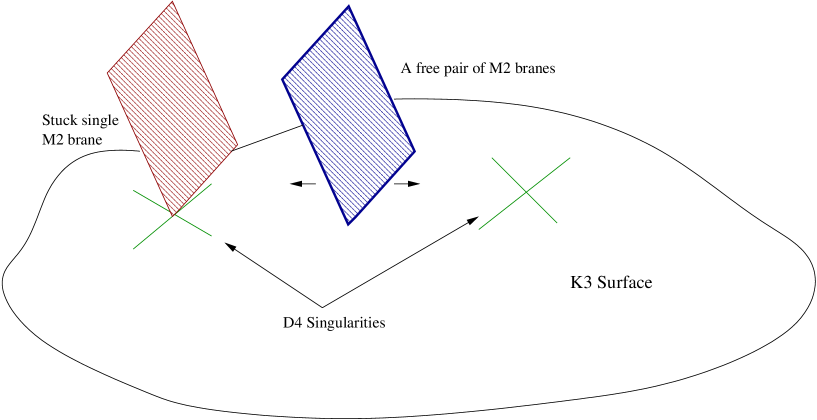
Figure 4: A depiction of the Coulomb branch for D5-branes wrapping $T^{3}$.

For $N$ odd, there are two isomorphic components in the moduli space. One M2-brane must bind two either of the $D_{4}$ singularities. The remaining branes wander in pairs over the $K3$ surface. This structure, arrived at by considering twisted $Sp(N)$ bundles on $T^{3}$, confirms a result found by a quite different argument in [46]: namely, that a membrane near a frozen $D_{4}$ singularity corresponds to instanton charge $2$ ($N=2$). We see quite explicitly that a charge $1$ instanton corresponds to a membrane trapped at the singularity.

This dictionary between M2-branes at frozen singularities, and the Coulomb branch of twisted wrapped 5-branes is quite critical for us. We shall use consistency with the results of [15, 46] to predict the Coulomb branch of the twisted $E_{8}$ tensor theory. The structure of the Coulomb branch can be described as follows: let us take $N$ $E_{8}$ 5-branes wrapping $T^{3}$ with a $p\over m$ twist. Let us further assume that the spacetime gauge symmetry is abelian. The dual description is M theory on a $K3$ with a pair of frozen $D_{4}$ singularities for $m=2$, $E_{6}$ singularities for $m=3$, $E_{7}$ singularities for $m=4$, and $E_{8}$ singularities for $m=5,6$. The value of $p$ determines the flux of the M theory $3$-form through the singularity. Consistency with [46] requires that a wandering membrane correspond to instanton charge $m$. We therefore split $N=p+p^{\prime}$ where $p$ M2-branes are localized at one singularity, while $p^{\prime}$ M2-branes live at the other singularity. If either $p\geq m$ or $p^{\prime}\geq m$ then $m$ branes can leave the singularity and wander into the bulk.

There is one final point that merits comment. For untwisted $T^{3}$ compactifications of $E_{8}$ 5-branes, which give theories with global $E_{6},E_{7}$ and $E_{8}$ symmetries, there exist mirror realizations. In the mirrors, the moduli space of instantons is realized on the Coulomb rather than the Higgs branch. These mirror descriptions can be constructed as the IR fixed points of the conventional $E_{6},E_{7}$ and $E_{8}$ quiver gauge theories [49]. For our twisted compactifications, the mirrors are currently unknown. It is not hard to see that in the IR, they correspond to the theories on coincident M2-branes localized at (partially) frozen $D_{4+n},E_{6},E_{7}$, and $E_{8}$ singularities. Depending on the choice of flux through the singularity, the global symmetry will correspond to the symmetry of table 1. Further the Coulomb branch will correspond to the appropriate moduli space of instantons, while the Higgs branch will correspond to the Coulomb branch described just above. Whether these theories can be given Lagrangian descriptions is an outstanding question.

3.4 Testing string/string duality

At this stage, we cannot resist applying our earlier results to string/string duality. Let us turn to the case of 5-branes wrapping $T^{4}$. Five-branes give rise to strings which we can interpret as fundamental strings of a dual description. The standard duality is between heterotic/type I on $T^{4}$ and type IIA on $K3$. Consider a IIA string wrapping the circle of $K3\times S^{1}$. The massless modes of the string correspond to states with $L_{0}=\bar{L}_{0}=0$, and there are $24$ such states corresponding to the cohomology of $K3$.

Let us recall how these light modes arise from a type I dual description. These states then correspond to light modes of a D5-brane wrapping $T^{4}\times S^{1}$. After T-dualizing on all circles, this system becomes $1$ D0-brane together with a collection of $32$ $\mathrm{O}4^{-}$-planes and $16$ pairs of D4-branes. The D0-brane sees $T^{5}/{\mathbb{Z}}_{2}$ as its moduli space. By correctly counting gauge invariant ground states, we see that there are $8$ light modes from motion on the moduli space [40]. There are no additional ground states from the D0-brane near an $\mathrm{O}4^{-}$-plane. These correspond to ground states in a pure $Sp(1)$ gauge theory with $8$ supercharges, but there are no such states [34, 35]. However, there is precisely one ground state from the D0-brane near each D4-brane [9]. This gives the required $16$ additional light modes.

The prior discussion assumes that the type I gauge bundle on $T^{4}$ is in the component of the moduli space containing the trivial Wilson line. It is natural to extend the analysis to the case of a NVS compactification. The dual description is IIA on a $K3$ surface with $8$ frozen $A_{1}$ singularities [16]. This is not really a perturbative string compactification because of the presence of torsion RR 1-form fluxes. However, it is essentially clear that a string wrapping an extra circle has $16$ rather than $24$ $L_{0}=\bar{L}_{0}=0$ light modes. The dual orientifold description now contains $24$ $\mathrm{O}4^{-}$-planes, $8$ $\mathrm{O}4^{+}$-planes, and $8$ D4-branes (see [15] for a discussion). From this description, we can determine the light degrees of freedom: again, there are $8$ modes from motion of the D0-brane on $T^{5}/{\mathbb{Z}}_{2}$, no modes from the $\mathrm{O}4^{-}$-planes and $8$ modes from the D4-branes. Using our result from section 2.3, we see that we also obtain no modes from the $\mathrm{O}4^{+}$-planes. In total, we obtain precisely $16$ modes, which is in accord with generalized string/string duality.

There is one more point worth stressing about IIA on a $K3$ with $8$ frozen $A_{1}$ singularities. As in all the cases we have considered, the non-simply-laced groups that appear in the low-energy theory imply the existence of fractional instantons. What is the stringy description for the small size limit of these instantons? As we have argued, a small (fractional) instanton in the dual heterotic theory on $T^{4}$ is a $5$-brane wrapping $T^{4}$. In the dual picture, these solitonic strings become fundamental strings of IIA. The duality dictionary therefore implies fractional strings localized at singularities. In this way, we rediscover the fractional strings of [16]. This argument, which only uses low-energy physics, complements the reasoning of [16] which appeals to M theory in order to predict fractional strings.

3.5 Quadruple and NVS compactifications

As a final topic in string/string duality, we will now briefly visit the case of $Spin(32)/{\mathbb{Z}}_{2}$ string theory on $T^{4}$. We will give a new argument for the equivalence of an NVS compactification with a quadruple compactification. A perturbative argument based on T-duality appears in [15]. Let us recall that a quadruple compactification corresponds to a gauge bundle in a disconnected component in the moduli space of flat connections on $T^{4}$. However, all possible CS invariants vanish. In particular, $Spin(32)/{\mathbb{Z}}_{2}$ admits a quadruple compactification.

To construct a quadruple, we first turn on Wilson lines on 2 of the 4 cycles available on $T^{4}$, such that a non-simply-connected group remains unbroken. According to the analysis by Schweigert [45], the twisted bundles with non-simply-connected structure groups on $T^{2}$ are related to diagram automorphisms of the extended Dynkin diagram. The groups we will encounter are of the $SO(4N)$ type; we therefore study the diagram automorphism of the extended diagram corresponding to $D_{2n}$.

Figure 5: The automorphisms which act on the extended Dynkin diagram of $D_{2n}$, and their correspondence with the quadruple and NVS compactifications.

There are two automorphisms that are relevant to us; see figure 5). We can flip the extended diagram from left to right, or up/down. The first corresponds to the no vector structure compactification; the second one gives the quadruple compactification.

Start with type I on $T^{4}$. Turn on 2 Wilson lines on 2 cycles such that the gauge group is broken to a manifest $O(8)^{4}$. From duality with the heterotic $Spin(32)/{\mathbb{Z}}_{2}$ string, it is not hard to deduce that the actual group is $Spin(8)^{4}/({\mathbb{Z}}_{2}\times{\mathbb{Z}}_{2})$. The ${\mathbb{Z}}_{2}\times{\mathbb{Z}}_{2}$ factor appearing in the quotient is the diagonal product of the centers of the 4 $Spin(8)$ factors. The two ${\mathbb{Z}}_{2}$ factors are related to the two diagram automorphisms we mentioned earlier.

Let us turn on a third Wilson line that breaks the (manifest) gauge group to $O(4)^{8}$. T-dualizing each direction of $T^{3}$ that carries a non-trivial Wilson line leads us to type IIA on $T^{3}/{\mathbb{Z}}_{2}\times S^{1}$. There are $8$ $\mathrm{O}6^{-}$-planes each with $2$ pairs of coincident D6-branes. This lifts to M theory on $T^{4}/{\mathbb{Z}}_{2}\times S^{1}$. We now have two interesting possibilities for the Wilson line around the extra circle: the first is to impose a holonomy on $S^{1}$ that exchanges the $O(4)$ groups in pairs. This reduces the rank by $8$, and results in an NVS compactification. The second possibility is to impose a holonomy that breaks each $O(4)\rightarrow O(3)\times O(1)$. This gives a quadruple compactification, and also reduces the rank by $8$.

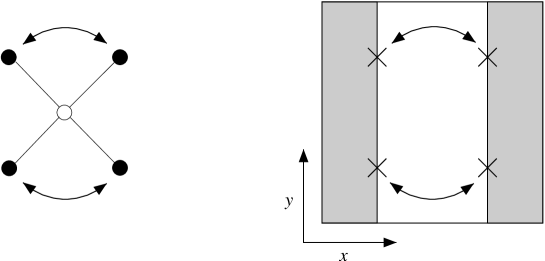
Figure 6: Geometry of the duality between NVS and the quadruple compactification. Left: the extended Dynkin diagram of $D_{4}$. Right: a fundamental domain for $({\mathbb{R}}^{2}\times T^{2})/{\mathbb{Z}}_{2}$.

Let us consider these theories after T-dualizing each cycle of $T^{3}$. It is sufficient for us to focus on $2$ $\mathrm{O}6^{-}$-planes and their associated $4$ pairs of D6-branes. In general $\mathrm{O}6^{-}$ with D6-branes lifts to a $D$-type singularity in M theory. In this case where there are only $2$ pairs of D6-branes, we obtain locally $4$ $A_{1}$ singularities, or $2$ “$D_{2}$” singularities. The explicit geometry in this case is $(R^{2}\times T^{2})/{\mathbb{Z}}_{2}$. Imposing the first flavor of Wilson line corresponds to exchanging pairs of $A_{1}$ singularities on traveling around the $S^{1}$. How about the second case? Reducing $O(4)\rightarrow O(3)\times O(1)$ requires a holonomy on $S^{1}$ with determinant $-1$. Conjugating by this holonomy is equivalent to acting by an outer automorphism, and so also corresponds to exchanging $2$ $A_{1}$ singularities in the M theory lift. However, the exchanged $A_{1}$ singularities now sit in the same fiber!

The M theory geometry is both simple and pretty, and is depicted in figure 6. On the left, we have the diagram of $D_{4}$, corresponding to $Spin(8)$. Breaking this to $O(4)^{2}$ corresponds to erasing the middle node. This should be compared with the right hand side, where we have depicted the $T^{2}/{\mathbb{Z}}_{2}$ which appears in $({\mathbb{R}}^{2}\times T^{2})/{\mathbb{Z}}_{2}$. The singularities, marked by crosses, just correspond to the black nodes of the Dynkin diagram on the left. The white node is the $T^{2}/{\mathbb{Z}}_{2}$ (which is topologically a 2-sphere) intersecting these singularities. The exchange of singularities depicted produces either an NVS or a quadruple compactification; it just depends whether on the right hand side we interpret the $x$ or the $y$ direction as the “eleventh” M theory direction. In other words, these two cases are related by a suitable $9-11$ flip. This provides a strong coupling version of the argument given in [15].

4 Domain Walls in Heterotic/Type I String Theory

The final topic that we shall discuss are domain walls in heterotic and type I string theory. In D=8 dimensions, there are two distinct $T^{2}$ type I/heterotic compactifications: the NVS compactification and the standard compactification. The gauge bundles are topologically distinct. Therefore there is no field theoretic domain wall that can smoothly interpolate between these two distinct vacua. However, as shall describe, there is a stringy domain wall that interpolates between these two vacua.

In $D=7$, there are many components in the heterotic string moduli space on $T^{3}$. These components are distinguished by the CS invariants of their $E_{8}\times E_{8}$ gauge bundles. The situation is nicer than in $D=8$ because the gauge bundles are all topologically trivial. As a starting point, we can then consider pure $E_{8}$ gauge theory on $T^{3}\times{\mathbb{R}}$. Let us parametrize ${\mathbb{R}}$ by a coordinate $x\in(-\infty,\infty).$ Consider an instanton configuration that interpolates between an $E_{8}$ gauge bundle with CS invariant, $CS(-\infty)$ at $x=-\infty$ to one with CS invariant, $CS(+\infty)$ at $x=\infty$. Such a BPS instanton is (generically) fractionally charged, satisfying:

$$\frac{1}{8\pi^{2}N_{R}}\int~{}\textrm{Tr}\,(F\wedge F)=CS(\infty)-CS(-\infty).$$ (43)

It is clear that there are smooth gauge-field configurations in a sector with fixed instanton charge. For example, a smooth interpolation between the flat gauge-field configurations at $x=\pm\infty$ works. What has yet to be shown is that smooth solutions exist which saturate the BPS bound $(\ref{instbound})$. The existence of such solutions might be demonstrated by extending the methods of [50, 51]. It might even be possible to explicitly construct such a solution using the connections worked out in [52]. This is an important issue in field theory, but less critical in string theory. A non-BPS configuration will decay down to something reasonable in string theory, and cannot decay away entirely because of its charge.

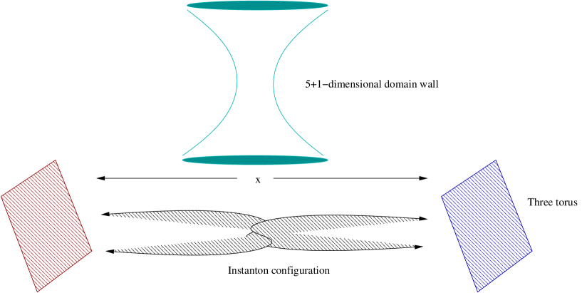
Figure 7: The embedded instanton/anti-instanton pair interpolate between fixed asymptotic CS invariants, giving a space-time domain wall.

When embedded in the heterotic string, we want to satisfy anomaly cancellation as $|x|\rightarrow\infty$ with $H_{3}=0$. From the usual relation,

$$H_{3}=dB_{2}+CS(\omega)-CS(A),$$ (44)

where $\omega$ is the spin connection, and $A$ the gauge-field, we see that we must embed a fractional instanton in one $E_{8}$ factor, and a fractional instanton of opposite charge in the second factor. The total configuration is then not BPS, although the instanton in each factor can be BPS. Since both vacua at $|x|=\infty$ are supersymmetric with zero cosmological constant, we do not expect static domain wall solutions when we couple gravity to our $E_{8}\times E_{8}$ Yang-Mills theory. Rather, the domain wall inflates. For a review of domain walls in supergravity, see [53].

4.1 Domain walls from orientifold planes

We start by constructing a domain wall for the $D=8$ case. Consider a stack of NS5-branes at a point on a four manifold, $M_{4}$. We can measure the 5-brane charge $k$ by computing

$$\int_{\partial M_{4}}H_{3}=k.$$ (45)

We want to introduce an orientifold plane in such a way that the NS5-branes are inside the world-volume of the plane. The orientifold projection inverts $B_{2}$, and therefore $H_{3}$. If we want to allow NS5-branes, we need to accompany the orientifold action with a geometrical action on the transverse space. This means that the orientifold plane has to be an O6 or an O8-plane. The case of an O6-plane is well-known, and has been studied in many configurations [54, 55, 56]. The case of interest for us is the $\mathrm{O}8^{-}$-plane. Although this plane does not make sense in isolation i.e. without additional D8-branes, we will soon make our local construction globally sensible.

Let us take our space $M_{4}$ to be ${\mathbb{R}}^{4}$. The $\mathrm{O}8^{-}$-plane intersects the $S^{3}=\partial{\mathbb{R}}^{4}$ on an $S^{2}$. We can now turn the $H_{3}$ integral into a $B_{2}$ integral over the boundary of the orientifolded $3$-sphere.

$$\int_{\partial({\mathbb{R}}^{3}\times{\mathbb{R}}/{\mathbb{Z}}_{2})}H_{3}=\int_{\partial({\mathbb{R}}^{3}\times{\mathbb{R}}/{\mathbb{Z}}_{2})}{d}B_{2}=\int_{\mathrm{O}8^{-}\bigcap S^{3}}B_{2}=k/2.$$ (46)

In particular, when $k$ is odd, the $\mathrm{O}8^{-}$-plane supports a half-integer $B_{2}$-flux on its world-volume (the same conclusion was reached in [57]).

Things are more interesting when the space transverse to the 5-branes is partially compactified. In particular, let us take $k$ NS5-branes at a point on $T^{2}\times{\mathbb{R}}^{2}$. We introduce an $\mathrm{O}8^{-}$-plane which wraps the $T^{2}$. The orientifolded space is now $(T^{2}\times{\mathbb{R}})\times{\mathbb{R}}/{\mathbb{Z}}_{2}$. Any transverse component of the $B_{2}$-field can be gauged away (provided the background is flat). We now repeat the previous argument, and compute

$$\int_{\partial(T^{2}\times{\mathbb{R}}\times{\mathbb{R}}/{\mathbb{Z}}_{2})}H_{3}=\int_{\partial(T^{2}\times{\mathbb{R}}\times{\mathbb{R}}/{\mathbb{Z}}_{2})}{d}B_{2}=\left(\int_{T^{2}}B_{2}\right)(\infty)-\left(\int_{T^{2}}B_{2}\right)(-\infty)=k/2,$$ (47)

where $\pm\infty$ refers to the boundary of ${\mathbb{R}}$. We see then that the stack of NS5-branes forms a domain wall. If we traverse the wall, the $B_{2}$-flux through the $T^{2}$ jumps by $k/2$ units. The most interesting case is when $k$ is odd. Necessarily, on one side of the domain wall we have an odd $B_{2}$-flux, while on the other side, we have an even $B_{2}$-flux. If there are $D8$-branes coincident with the $\mathrm{O}8^{-}$-plane, we can now invoke the arguments of [42, 43]. On one side of the domain wall, we have vector structure on the two-torus, while on the other side we do not. Note that it is absolutely crucial for this argument that the NS5-branes are effectively codimension 1 with respect to the $\mathrm{O}8^{-}$-plane. Otherwise, we do not have a domain wall. Studying the effect of T-duality on this configuration should be interesting.

We will take a different tact, and replace ${\mathbb{R}}/{\mathbb{Z}}_{2}$ by $S^{1}/{\mathbb{Z}}_{2}$. Forgetting the NS5-branes for the moment, the resulting configuration is type I’ on $S^{1}/{\mathbb{Z}}_{2}\times T^{2}$. With a single T-duality, we could arrive at type I on $T^{3}$. We, however, are interested in the M theory description of this setup so we perform a 9-11 flip, compactifying from M theory to IIA on $S^{1}/{\mathbb{Z}}_{2}$. This gives the Horava-Witten theory on a three-torus [58]. The NS5-branes become heterotic M theory 5-branes, while the $B_{2}$ fluxes become $C_{3}$ fluxes.

Combined with the arguments given in [15], and the connection between 5-branes and small instantons in heterotic string theory, we are inevitably lead to the conclusion that we have found a domain wall. It interpolates between two $E_{8}$ vacua: one is the standard $T^{3}$ compactification, while the other is a ${\mathbb{Z}}_{2}$ triple. When crossing the interval between the two HW walls, the $C_{3}$-field cannot jump. This is achieved by embedding a second domain wall in the other HW wall. This configuration corresponds precisely to the fractional instanton solution that we expected to find.

In the strong coupling limit, the HW walls are far apart, and the $E_{8}$ groups are localized at each wall. In the weak coupling limit, when the HW walls come close together, the picture of localized gauge groups is no longer accurate, but happily, the picture of localized 5-branes cannot be trusted either. Instead it seems likely that the two oppositely charged 5-branes form a non-BPS configuration that is smeared along the interval between the 5-branes. Although there seems to be no direct link, a parallel with the behaviour of the non-BPS string of type I’ as a function of the distance between the $\mathrm{O}8^{-}$-planes [59] is very suggestive.

4.2 Beyond $T^{3}$

Much of our discussion should extend to lower-dimensional compactifications. Type I on $T^{4}$ has a number of distinct vacua again distinguished by the choice of gauge bundle. Of particular interest is the quadruple compactification. This bundle cannot be smoothly deformed away, yet there is no topological class that characterizes the bundle. It is natural for us to conjecture that Yang-Mills theory on $T^{4}\times{\mathbb{R}}$ has finite action field configurations that interpolate between the quadruple and the trivial vacuum. There is no natural candidate for a quantum number that can characterize this configuration so we expect it to be non-BPS. When embedded in string theory, the domain wall corresponds to a non-BPS $4$-brane. Interpreting the domain wall from the perspective of the string worldsheet is quite intriguing because it involves unwinding a discrete RR 4-form flux [20]. There will also be cases where NVS compactifications are combined with quadruples to give new kinds of domain walls.

The situation is similar for $T^{5}$ where there exist quintuple compactifications of the $E_{8}\times E_{8}$ string. Again there should be concomitant domain wall solutions, which now correspond to non-BPS $3$-branes. In this case, we can embed a quintuple in either $E_{8}$, or in both factors, so there are at least two distinct domain walls.

For type I on $T^{6}$ (or any $6$-dimensional Calabi-Yau compactification), something new should happen. There are $2$ classes of compactification which are distinguished by a discrete NS-NS $B_{6}$ flux [21]. As we approach a domain wall, which will be a membrane in the $4$ space-time dimensions, the field strength $H_{7}=dB_{6}$ will vary. Note that $H_{7}$ is supported in the $6$ internal space coordinates, and along the spatial direction transverse to the domain wall. However, $H_{3}=\ast H_{7}$, so from the perspective of a fundamental string, there is a varying electric flux. This suggests the intriguing possibility that space-time non-commutativity might be involved.

5 Acknowledgements

It is our pleasure to thank P. van Baal, N. Dorey, A. Hanany, A. Hashimoto, K. Hori, S. Ross, E. Witten, and P. Yi for helpful discussions. We would also like to thank the organizers of the Amsterdam 2001 Summer Workshop where we initiated this project. The work of A. K. is supported in part by EU contract HPRN-CT-2000-00122, while the work of S. S. is supported in part by NSF CAREER Grant No. PHY-0094328, and by the Alfred P. Sloan Foundation.

Appendix A Symplectic Group Actions

We will summarize some useful relations between quaternions and symplectic groups. Let us label a basis for our quaternions by $\{{\bf 1},I,J,K\}$ where,

$$I^{2}=J^{2}=K^{2}=-{\bf 1},\qquad IJK=-{\bf 1}.$$

A quaternion $q$ can then be expanded in components

$$q=q^{1}+Iq^{2}+Jq^{3}+Kq^{4}.$$

The conjugate quaternion $\bar{q}$ has an expansion

$$\bar{q}=q^{1}-Iq^{2}-Jq^{3}-Kq^{4}.$$

The symmetry group $Sp(1)_{R}\sim SU(2)_{R}$ is the group of unit quaternions.

Right multiplication by $I$ on $q$ gives

$$q \,\rightarrow\, qI$$ (48)

$$\,\rightarrow\, q^{1}I-q^{2}-q^{3}K+q^{4}J,$$ (49)

which can be realized by the matrix

$$I^{R}=\pmatrix{0&-1&0&0\cr 1&0&0&0\cr 0&0&0&1\cr 0&0&-1&0}$$ (50)

acting on $q$ in the usual way $q_{a}\,\rightarrow\,I^{R}_{ab}\,q_{b}$. The matrices $J^{R}$ and $K^{R}$ realize right multiplication by $J,K$ while ${\bf{1}}^{R}$ is the identity matrix:

$$J^{R}=\pmatrix{0&0&-1&0\cr 0&0&0&-1\cr 1&0&0&0\cr 0&1&0&0},\qquad K^{R}=\pmatrix{0&0&0&-1\cr 0&0&1&0\cr 0&-1&0&0\cr 1&0&0&0}.$$ (51)

Fianlly, we define operators $s^{j}$ in terms of $\left\{{\bf{1}}^{R},I^{R},J^{R},K^{R}\right\}$

$$s^{1}=\pmatrix{\bf{1}^{R}&0\cr 0&\bf{1}^{R}},\quad s^{2}=\pmatrix{I^{R}&0\cr 0&I^{R}},\quad s^{3}=\pmatrix{J^{R}&0\cr 0&J^{R}},\quad s^{4}=\pmatrix{K^{R}&0\cr 0&K^{R}}.$$

We will use the $s^{j}$ for the quaternion basis, and write a quaternion simply as

$$a\equiv s^{j}a_{j}$$

This facilitates both notation, and computation. Note however that in this formalism a quaternion is an $8\times 8$ matrix acting to the right. If we want it to act to the left, we need to take the transpose, which is easily seen to correspond to quaternionic conjugation, which we denote with a bar. As an example:

$$s^{j}_{ab}q_{j}s^{k}_{cd}p_{k}\delta_{bd}\rightarrow q\bar{p}$$

Note that a combination like $a\bar{a}\equiv|a|^{2}$ is actually a real number, multiplying the $8\times 8$ identity matrix.

Finally, we introduce gamma matrices

$$\gamma^{1}=\pmatrix{0&1\cr 1&0}\qquad\gamma^{2}=\pmatrix{0&I\cr-I&0}\qquad\gamma^{3}=\pmatrix{0&J\cr-J&0}$$

$$\gamma^{4}=\pmatrix{0&K\cr-K&0}\qquad\gamma^{5}=\pmatrix{1&0\cr 0&-1}$$

with $1,I,J,K$ a realization of the quaternion algebra in terms of $4\times 4$ real anti-symmetric matrices

$$I=\pmatrix{0&\sigma^{1}\cr-\sigma^{1}&0}\qquad J=\pmatrix{-i\sigma^{2}&0\cr 0&-i\sigma^{2}}\qquad K=\pmatrix{0&\sigma^{3}\cr-\sigma^{3}&0}\qquad$$

where $\sigma^{i}$ are the Pauli matrices.

References

- [1]
- [2] O. J. Ganor and A. Hanany, “Small Instantons and Tensionless Non-critical Strings,” Nucl. Phys. B 474, 122 (1996) [arXiv:hep-th/9602120].
- [3] N. Seiberg and E. Witten, “Comments on String Dynamics in Six Dimensions,” Nucl. Phys. B 471, 121 (1996) [arXiv:hep-th/9603003].
- [4] O. J. Ganor, “Toroidal compactification of heterotic 6D non-critical strings down to four dimensions,” Nucl. Phys. B 488, 223 (1997) [arXiv:hep-th/9608109].
- [5] O. J. Ganor, D. R. Morrison and N. Seiberg, “Branes, Calabi-Yau spaces, and toroidal compactification of the N = 1 six-dimensional E(8) theory,” Nucl. Phys. B 487, 93 (1997) [arXiv:hep-th/9610251].
- [6] K. A. Intriligator, “Compactified little string theories and compact moduli spaces of vacua,” Phys. Rev. D 61, 106005 (2000) [arXiv:hep-th/9909219].
- [7] G. ’t Hooft, “A Property Of Electric And Magnetic Flux In Nonabelian Gauge Theories,” Nucl. Phys. B 153, 141 (1979).
- [8] S. Sethi and M. Stern, “Invariance theorems for supersymmetric Yang-Mills theories,” Adv. Theor. Math. Phys. 4, 487 (2000) [arXiv:hep-th/0001189].
- [9] S. Sethi and M. Stern, “A comment on the spectrum of H-monopoles,” Phys. Lett. B 398, 47 (1997) [arXiv:hep-th/9607145].
- [10] N. Dorey, T. J. Hollowood and V. V. Khoze, “The D-instanton partition function,” JHEP 0103, 040 (2001) [arXiv:hep-th/0011247].
- [11] N. Dorey, T. J. Hollowood and V. V. Khoze, “Notes on soliton bound-state problems in gauge theory and string theory,” arXiv:hep-th/0105090.
- [12] C. J. Kim, K. M. Lee and P. Yi, “DLCQ of fivebranes, large N screening, and L**2 harmonic forms on Calabi manifolds,” Phys. Rev. D 65, 065024 (2002) [arXiv:hep-th/0109217].
- [13] G. W. Moore, N. Nekrasov and S. Shatashvili, “D-particle bound states and generalized instantons,” Commun. Math. Phys. 209, 77 (2000) [arXiv:hep-th/9803265].
- [14] M. Staudacher, “Bulk Witten indices and the number of normalizable ground states in supersymmetric quantum mechanics of orthogonal, symplectic and exceptional groups,” Phys. Lett. B 488, 194 (2000) [arXiv:hep-th/0006234].
- [15] J. de Boer, R. Dijkgraaf, K. Hori, A. Keurentjes, J. Morgan, D. R. Morrison and S. Sethi, “Triples, fluxes, and strings,” arXiv:hep-th/0103170.
- [16] J. H. Schwarz and A. Sen, “Type IIA dual of the six-dimensional CHL compactification,” Phys. Lett. B 357, 323 (1995) [arXiv:hep-th/9507027].
- [17] A. Sen, “Non-BPS D-Branes In String Theory,” Class. Quant. Grav. 17, 1251 (2000); “Non-BPS States and Branes in String Theory,” arXiv:hep-th/9904207.
- [18] A. Vilenkin, “Gravitational Field Of Vacuum Domain Walls,” Phys. Lett. B 133, 177 (1983).
- [19] H. Singh, “Romans type IIA theory and the heterotic strings,” arXiv:hep-th/0201206.
- [20] A. Keurentjes, “Discrete moduli for type I compactifications,” Phys. Rev. D 65, 026007 (2002) [arXiv:hep-th/0105101].
- [21] D. R. Morrison and S. Sethi, “Novel type I compactifications,” arXiv:hep-th/0109197.
- [22] S. Kachru, X. Liu, M. Schulz and S. P. Trivedi, “Supersymmetry Changing Bubbles in String Theory,” arXiv:hep-th/0205108.
- [23] R. Bott, “An Application Of Morse Theory To The Topology Of Lie Groups,” Bull. Soc. Math. Fr. 84 (1956) 251.
- [24] E. B. Dynkin, “Semisimple Subalgebras Of Semisimple Lie Algebras,” Trans. Am. Math. Soc. 6 (1957) 111.
- [25] M. A. Shifman and A. I. Vainshtein, “On Gluino Condensation In Supersymmetric Gauge Theories. SU(N) And O(N) Groups,” Nucl. Phys. B 296 (1988) 445 [Sov. Phys. JETP 66 (1988) 1100].
- [26] A. Y. Morozov, M. A. Olshanetsky and M. A. Shifman, Sov. Phys. JETP 67 (1988) 222 [Nucl. Phys. B 304 (1988) 291, Zh. Eksp. Teor. Fiz.94:18-32,1988].
- [27] K. R. Dienes, “String Theory and the Path to Unification: A Review of Recent Developments,” Phys. Rept. 287, 447 (1997) [arXiv:hep-th/9602045].
- [28] A. Borel, R. Friedman and J. W. Morgan, “Almost commuting elements in compact Lie groups,” arXiv:math.gr/9907007.
- [29] S. Chaudhuri, G. Hockney and J. D. Lykken, “Maximally supersymmetric string theories in ,” Phys. Rev. Lett. 75, 2264 (1995) [arXiv:hep-th/9505054].
- [30] C. W. Bernard, N. H. Christ, A. H. Guth and E. J. Weinberg, “Pseudoparticle Parameters For Arbitrary Gauge Groups,” Phys. Rev. D 16, 2967 (1977).
- [31] A. Hanany and J. Troost, “Orientifold planes, affine algebras and magnetic monopoles,” JHEP 0108 (2001) 021 [arXiv:hep-th/0107153].
- [32] K. Hori, “D-branes, T-duality, and index theory,” Adv. Theor. Math. Phys. 3, 281 (1999) [arXiv:hep-th/9902102].
- [33] S. Sethi and M. Stern, “The structure of the D0-D4 bound state,” Nucl. Phys. B 578, 163 (2000) [arXiv:hep-th/0002131].
- [34] S. Sethi and M. Stern, “D-brane bound states redux,” Commun. Math. Phys. 194 (1998) 675 [arXiv:hep-th/9705046].
- [35] P. Yi, “Witten index and threshold bound states of D-branes,” Nucl. Phys. B 505, 307 (1997) [arXiv:hep-th/9704098].
- [36] N. H. Christ, E. J. Weinberg and N. K. Stanton, “General Self-Dual Yang-Mills Solutions,” Phys. Rev. D 18 (1978) 2013.
- [37] O. Aharony, S. Kachru and E. Silverstein, “New N = 1 superconformal field theories in four dimensions from D-brane probes,” Nucl. Phys. B 488, 159 (1997) [arXiv:hep-th/9610205].
- [38] K. A. Intriligator, “New string theories in six dimensions via branes at orbifold singularities,” Adv. Theor. Math. Phys. 1, 271 (1998) [arXiv:hep-th/9708117].
- [39] J. D. Blum and K. A. Intriligator, “New phases of string theory and 6d RG fixed points via branes at orbifold singularities,” Nucl. Phys. B 506, 199 (1997) [arXiv:hep-th/9705044].
- [40] E. Witten, “Small Instantons in String Theory,” Nucl. Phys. B 460, 541 (1996) [arXiv:hep-th/9511030].
- [41] E. Witten, “Toroidal compactification without vector structure,” JHEP 9802, 006 (1998) [arXiv:hep-th/9712028].
- [42] M. Bianchi, G. Pradisi and A. Sagnotti, “Toroidal compactification and symmetry breaking in open string theories,” Nucl. Phys. B 376, 365 (1992).
- [43] A. Sen and S. Sethi, “The mirror transform of type I vacua in six dimensions,” Nucl. Phys. B 499, 45 (1997) [arXiv:hep-th/9703157].
- [44] A. Keurentjes, “Orientifolds and twisted boundary conditions,” Nucl. Phys. B 589, 440 (2000) [arXiv:hep-th/0004073].
- [45] C. Schweigert, “On moduli spaces of flat connections with non-simply connected structure group,” Nucl. Phys. B 492, 743 (1997) [arXiv:hep-th/9611092].
- [46] M. Atiyah and E. Witten, “M-theory dynamics on a manifold of G(2) holonomy,” arXiv:hep-th/0107177.
- [47] K. Dasgupta and S. Mukhi, JHEP 9907 (1999) 008 [arXiv:hep-th/9904131].
- [48] P. K. Townsend, “D-branes from M-branes,” Phys. Lett. B 373 (1996) 68 [arXiv:hep-th/9512062].
- [49] K. A. Intriligator and N. Seiberg, “Mirror symmetry in three dimensional gauge theories,” Phys. Lett. B 387, 513 (1996) [arXiv:hep-th/9607207].
- [50] M. Jardim, “Classification and existence of doubly-periodic instantons,” arXiv:math.dg/0108004.
- [51] C. Ford, J. M. Pawlowski, T. Tok and A. Wipf, “ADHM construction of instantons on the torus,” Nucl. Phys. B 596, 387 (2001) [arXiv:hep-th/0005221].
- [52] K. G. Selivanov and A. V. Smilga, “Classical Yang-Mills vacua on T(3): Explicit constructions,” Phys. Rev. D 63, 125020 (2001) [arXiv:hep-th/0010243].
- [53] M. Cvetic and H. H. Soleng, “Supergravity domain walls,” Phys. Rept. 282, 159 (1997) [arXiv:hep-th/9604090].
- [54] N. Evans, C. V. Johnson and A. D. Shapere, “Orientifolds, branes, and duality of 4D gauge theories,” Nucl. Phys. B 505, 251 (1997) [arXiv:hep-th/9703210].
- [55] A. Hanany and B. Kol, “On orientifolds, discrete torsion, branes and M theory,” JHEP 0006, 013 (2000) [arXiv:hep-th/0003025].
- [56] G. Bertoldi, B. Feng and A. Hanany, “The splitting of branes on orientifold planes,” JHEP 0204, 015 (2002) [arXiv:hep-th/0202090].
- [57] C. Bachas, N. Couchoud and P. Windey, “Orientifolds of the 3-sphere,” JHEP 0112, 003 (2001) [arXiv:hep-th/0111002].
- [58] P. Horava and E. Witten, “Heterotic and type I string dynamics from eleven dimensions,” Nucl. Phys. B 460, 506 (1996) [arXiv:hep-th/9510209].
- [59] T. Dasgupta and B. J. Stefanski, “Non-BPS states and heterotic - type I’ duality,” Nucl. Phys. B 572 (2000) 95 [arXiv:hep-th/9910217].