D-branes in asymmetrically gauged WZW models
and axial-vector duality

Mark A. Walton and Jian-Ge Zhou

Physics Department, University of Lethbridge, Lethbridge, Alberta, Canada T1K 3M4

Abstract

We construct D-branes in a left-right asymmetrically gauged WZW model, with the gauge subgroup embedded differently on the left and the right of the group element. The symmetry-preserving boundary conditions for the group-valued field $g$ are described, and the corresponding action is found. When the subgroup $H=U(1)$, we can implement T-duality on the axially gauged WZW action; an orbifold of the vectorially gauged theory is produced. For the parafermion $SU(2)/U(1)$ coset model, a $\sigma$-model is obtained with vanishing gauge field on D-branes. We show that a boundary condition surviving from the $SU(2)$ parent theory characterizes D-branes in the parafermion theory, determining the shape of A-branes. The gauge field on B-branes is obtained from the boundary condition for A-branes, by the orbifold construction and T-duality. These gauge fields stabilize the B-branes.

PACS: 11.25.Hf, 11.25.-w

1 Introduction

The pioneering work of Maldacena, Moore and Seiberg [1] initiated the study of the geometry of D-branes in coset models [2]-[8]. The bosonic theory they focused on was the parafermion $SU(2)/U(1)$ coset model. A-branes were studied using rational conformal field theory (CFT) via the Cardy construction. By $\mbox{$ZZ$}_{k}$-orbifolding and T-duality, B-branes were also obtained.

In [2][3], it was shown that A-branes can be given a geometrical interpretation in the vectorially gauged Wess-Zumino-Witten (WZW) model [9][10]. There the boundary value of the group-valued field $g$ was found to be in a product of two conjugacy classes – one of $G$ and the other of $H$. This boundary form was justified in [7], where it was derived from the corresponding gluing conditions. The non-commutative gauge theories dictating the dynamics of D-branes in $G/H$ coset models were constructed in [5].

There is a one-to-one Cardy correspondence between A-type boundary states and bulk primary fields in the $SU(2)/U(1)$ parafermion theory [1]. For B-branes the Cardy correspondence does not hold, and so we have less understanding of B-branes than A-branes. For instance, it is unclear how to decide if B-branes are stable and if they can be described by some kind of gauged WZW model. From the construction of B-branes in [1], it seems that B-branes are related to the axially gauged WZW model. For open strings, however, only the vectorially gauged WZW model [2][3][7] has been treated. It is interesting therefore to study D-branes in left-right asymmetrically gauged WZW models, including axially gauged WZW models as special cases.

When the gauge subgroup is abelian, there is an axial-vector duality [11][12] in the coset model for closed strings. Considered as $\sigma$-models, the axial and vector gauging of an abelian chiral symmetry leads to different target spaces; one may even be singular when the other is regular [11]. The corresponding axially and vectorially gauged WZW models describe the same coset CFT, however.  One may wonder whether there is an axial-vector duality in the coset model for open strings.

Here we discuss D-branes in the left-right asymmetrically gauged WZW models, with different embeddings of the same gauge subgroup acting on the left and on the right. We construct the left-right asymmetrically gauged WZW action for open strings, and find the boundary condition for group-valued field $g$ which preserves the left-right asymmetric symmetry. The methods of [7] make this straightforward.

When the subgroup $H$ is abelian, we obtain the axially gauged WZW action. We then implement T-duality to get the vectorially gauged WZW action. When we do T-duality, we find there is a crucial change of the boundary condition for the $U(1)$ coordinate $X$ and its dual $\tilde{X}$. The angle $X$ that parametrizes the $U(1)$ subgroup takes values in $[0,2\pi]$, but the range of values of the dual angle $\tilde{X}$ is instead $[0,\frac{2\pi}{k}]$. This is because the axially gauged WZW model is T-dual to the $\mbox{$ZZ$}_{k}$ orbifold of the vectorially gauged WZW model.

After constructing D-branes in left-right asymmetrically gauged WZW model, we specialize to the $SU(2)/U(1)$ coset model, described by a vectorially gauged WZW model. From the WZW action, we obtain a $\sigma$-model with vanishing gauge field on D-branes. Since the geometry of the resulting disk is conformally flat and the gauge field on D-branes vanishes, the remaining boundary condition for D-branes in the $SU(2)$ parent theory carries over to the coset model. From this, we see that the shape of an A-brane in the $SU(2)/U(1)$ coset model is a straight line. This observation is supported by scattering amplitudes between the boundary states for A-branes and the closed string states [16][1]. In the parafermion theory there is global $U(1)$ symmetry, but the consistency of the gauged WZW model for open strings does not demand that the $U(1)$ parameter be quantized [7]. If we insist on the Cardy correspondence, the scattering amplitudes between the boundary states for A-branes and the closed string states indicate that the $U(1)$ symmetry has to be broken to $\mbox{$ZZ$}_{2k}$ symmetry. That is, only the $2k$ points in a single $\mbox{$ZZ$}_{2k}$ orbit on the disk boundary are valid as endpoints of A1-branes. The selection rule eliminates half of these endpoints, and we are left with a $\mbox{$ZZ$}_{k}$ symmetry.

Since the resulting $\sigma$-model possesses $\mbox{$ZZ$}_{k}$ symmetry, we construct its $\mbox{$ZZ$}_{k}$ orbifold. Then we can implement T-duality. We find that the original conformally flat disk is mapped to another conformally flat disk, and the gauge field on B-branes can be obtained from the boundary condition for A-branes. The resulting $\sigma$-model yields the boundary condition for B-branes, showing that their shapes are centered disks. In addition, we find gauge field strengths that stabilize the B-branes – according to [1], they prevent the B-branes from decaying by shrinking or by displacing off the center. Finally, the $\sigma$-model action for B-branes can be recast into the axially gauged WZW action. This manifests the axial-vector duality in the $SU(2)/U(1)$ coset model for open strings.

The layout of this paper is as follows. In section 2 we discuss D-branes in the asymmetrically gauged WZW model, and construct the corresponding action for open strings. We also show how axial-vector duality can be realized in this model. In section 3 we consider the vectorially $U(1)$-gauged WZW model for open strings. We extract the boundary conditions for A-branes in the $SU(2)/U(1)$ coset model for open strings, and compare them with results obtained from the scattering amplitudes between the boundary states for A-branes and the closed string states. We obtain the $\sigma$-model for B-branes in section 4, by constructing the theory T-dual to an orbifold of that describing A-branes. Consequently, the gauge field on B-branes is calculated from the boundary conditions for A-branes. Also discussed is the axial-vector duality in the $SU(2)/U(1)$ coset model for open strings. In section 5 we present our summary and discussion.

2 D-branes in asymmetrically gauged WZW models

To describe our notation, we start with the vectorially gauged WZW model for open strings. Let $G$ be a compact, simply connected, Lie group. The $G/H$ coset CFT, where $H$ is a subgroup of $G$, can be described by a gauged WZW action with the vector symmetry

$$g\rightarrow vgv^{-1}$$ (1)

gauged away. Here $g\in G$ and $v\in H\subset G$.

For closed strings, the gauged WZW action is [9],[10]

$$S^{G/H}\ =\ S(U^{-1}g\tilde{U})-S(U^{-1}\tilde{U})\ =\ S({\hat{g}})-S(h)\ ,$$ (2)

with

$${\hat{g}}=U^{-1}g\tilde{U}\in G,\ \ \ \ h=U^{-1}\tilde{U}\in H,\ \ \ \ g\in G,\ \ \ \ U,\tilde{U}\in H$$ (3)

and gauge fields

$$A_{z}=\partial_{z}\tilde{U}\tilde{U}^{-1},\ \ \ \ A_{\bar{z}}=\partial_{\bar{z}}UU^{-1}\ .$$ (4)

Here $S$ is the WZW action for the group $G$.

The Wess-Zumino term (part of the WZW action) is not well-defined for a worldsheet $\Sigma$ with a boundary, however. The remedy is to introduce an auxiliary disk $D$ for each hole in $\Sigma$ with boundaries common with those of $\Sigma$ [17]. For simplicity, we consider the situation with a single hole. The map $g$ from $\Sigma$ to $G$ is then extended to a map from the extended worldsheet $\Sigma\cup D$. The disk $D$ is mapped to the product of two conjugacy classes for $G$ and $H$. Then [2][3][7]

$$S^{G/H} = \frac{k}{4\pi}\left(\int_{\Sigma}d^{2}z\,L^{\rm kin}({\hat{g}})+\int_{B}\chi({\hat{g}})-\int_{D}\omega({\hat{g}})\right)$$ (5)

$$- \frac{k_{H}}{4\pi}\left(\int_{\Sigma}d^{2}z\,L^{\rm kin}(h)+\int_{B}\chi(h)-\int_{D}\omega(h)\right)\ ,$$

is the gauged WZW action for open strings. Here $B$ is a three-dimensional manifold bounded by $\Sigma\cup D$. $\omega({\hat{g}})$ and $\omega(h)$ are the Alekseev-Schomerus two-forms defined on the conjugacy classes of $G$ and $H$, respectively.

In the form most useful to us, the action of the vectorially gauged WZW model for open string is [2][3][7]

$$S^{G/H} = \frac{k}{4\pi}\left(\int_{\Sigma}d^{2}z\,L^{\rm kin}(g)+\int_{B}\chi(g)\right)$$ (6)

$$+ \frac{k}{2\pi}\int_{\Sigma}d^{2}z\,tr\left\{A_{z}\partial_{\bar{z}}gg^{-1}-A_{\bar{z}}g^{-1}\partial_{z}g+A_{z}gA_{\bar{z}}g^{-1}-A_{z}A_{\bar{z}}\right\}$$

$$- \frac{k}{4\pi}\int_{D}\,\left\{\Omega(n;{\underline{f}})+\Omega(p;{\underline{l}})+tr(dc_{H}c_{H}^{-1}c_{G}^{-1}dc_{G})\right\}$$

where $B$ is a three-dimensional manifold bounded by $\Sigma\cup D$, i.e. $\partial B=\Sigma\cup D$. $c_{G}$ and $c_{H}$ are elements of fixed conjugacy classes of $G$ and $H$, respectively. More precisely, let $\tau$ parametrize the boundary $\partial\Sigma=-\partial D$. We write $c_{G}=n(\tau){\underline{f}}n(\tau)^{-1}$ with ${\underline{f}},n\in G$. The underline of ${\underline{f}}$ indicates it is a fixed element, independent of $\tau$. Similarly, we write $c_{H}=p(\tau){\underline{l}}p(\tau)^{-1}$, ${\underline{l}},p\in H$, with ${\underline{l}}$ fixed. The two-forms $\Omega$ are defined by

$$\Omega(n;{\underline{f}})=tr(n^{-1}dn{\underline{f}}n^{-1}dn{\underline{f}}^{-1}),\ \ \ \ \Omega(p;{\underline{l}})=tr(p^{-1}dp{\underline{l}}p^{-1}dp{\underline{l}}^{-1})\ \ .$$ (7)

Finally, $L^{\rm kin}(g)=tr(\partial_{z}g\partial_{\bar{z}}g^{-1})$, $\chi(g)=\frac{1}{3}tr(dgg^{-1})^{3}$. These latter satisfy the Polyakov-Wiegmann identities

$$L^{\rm kin}(g_{1}g_{2})=L^{\rm kin}(g_{1})+L^{\rm kin}(g_{2})-tr(g_{1}^{-1}\partial_{z}g_{1}\partial_{\bar{z}}g_{2}g_{2}^{-1}+g_{1}^{-1}\partial_{\bar{z}}g_{1}\partial_{z}g_{2}g_{2}^{-1})$$

$$\chi(g_{1}g_{2})=\chi(g_{1})+\chi(g_{2})-d\,tr(g_{1}^{-1}dg_{1}\,dg_{2}g_{2}^{-1})\ \ .$$ (8)

The boundary value of $g\in G$ is [2][3][7]

$$g(\tau)\ =\ c_{G}\,c_{H}\ =\ n{\underline{f}}n^{-1\,}p{\underline{l}}p^{-1}(\tau)$$ (9)

where, again, ${\underline{f}}$ and ${\underline{l}}$ have no $\tau$-dependence. We can write ${\underline{f}}=e^{2\pi i\lambda_{G}/k}$ and ${\underline{l}}=e^{2\pi i\lambda_{H}/k_{H}}$, where $\lambda_{G}$ and $\lambda_{H}$ are elements of the Cartan subalgebras of the Lie algebras of $G$ and $H$. The single-valuedness of path integrals involving the action (6) leads to the quantization conditions [2][3]

$$\alpha_{G}(\lambda_{G})\in\mbox{$ZZ$}$$ (10)

$$\alpha_{H}(\lambda_{H})\in\mbox{$ZZ$}$$ (11)

for any coroots $\alpha_{G}$ and $\alpha_{H}$ of the Lie algebras of $G$ and $H$. When $H$ is an abelian subgroup, the second condition (11) does not apply.

To construct the left-right asymmetrically gauged WZW action for open strings, we first recall some results for closed strings [18] (see also [20][21], e.g.). Introduce the gauge fields $A$ and $\tilde{A}$ as

$$A_{z}=T_{a}A_{z}^{a},\ \ \ A_{\bar{z}}=T_{a}A_{\bar{z}}^{a},\ \ \ \tilde{A}_{z}=\tilde{T}_{a}A_{z}^{a},\ \ \ \tilde{A}_{\bar{z}}=\tilde{T}_{a}A_{\bar{z}}^{a}\ \ .$$ (12)

Notice that $A_{z}$, $A_{\bar{z}}$ are independent gauge fields. On the other hand, $\tilde{A}_{z}$, $\tilde{A}_{\bar{z}}$ are related to $A_{z}$, $A_{\bar{z}}$, respectively – they only differ because $T_{a}$, $\tilde{T}_{a}$ indicate possibly different embeddings of a generator of the Lie algebra of the subgroup $H$. These must obey the constraints [18]

$$tr(T_{a}[T_{b},T_{c}])=tr(\tilde{T}_{a}[\tilde{T}_{b},\tilde{T}_{c}]),\ \ \ \ tr(T_{a}T_{b})=tr(\tilde{T}_{a}\tilde{T}_{b})\ \ .$$ (13)

Actually, the second constraint guarantees the first, and means the two embeddings of $H$ in $G$ must have the same index.

The left-right asymmetrical transformations are defined as [18]

$$g\rightarrow mg{\tilde{m}}^{-1}$$ (14)

$$A_{z}\rightarrow m{A_{z}}m^{-1}+\partial_{z}m\,m^{-1},$$

$$A_{\bar{z}}\rightarrow mA_{\bar{z}}m^{-1}+\partial_{\bar{z}}m\,m^{-1},$$

$${\tilde{A}}_{z}\rightarrow\tilde{m}{\tilde{A}}_{z}\tilde{m}^{-1}+\partial_{z}\tilde{m}\,\tilde{m}^{-1},$$

$${\tilde{A}}_{\bar{z}}\rightarrow\tilde{m}{\tilde{A}}_{\bar{z}}\tilde{m}^{-1}+\partial_{\bar{z}}\tilde{m}\,\tilde{m}^{-1}.$$ (15)

We write $m\in H_{L}\subset G$, and ${\tilde{m}}\in H_{R}\subset G$, for obvious reasons.

The action [18]

$$S^{G/H}=S+\frac{k}{4\pi}\int_{\Sigma}d^{2}z\,tr\left\{2A_{z}\partial_{\bar{z}}gg^{-1}-2\tilde{A}_{\bar{z}}g^{-1}\partial_{z}g+2A_{z}g\tilde{A}_{\bar{z}}g^{-1}-A_{z}A_{\bar{z}}-\tilde{A}_{z}\tilde{A}_{\bar{z}}\ .\right\}$$ (16)

is invariant under the left-right asymmetrical transformations (14) and (15). In [19], this asymmetrically gauged WZW action (16) for closed strings was used to remove axial $U(1)$ subgroup degrees of freedom.

We introduce the subgroup valued world sheet fields $U,U^{{}^{\prime}}\in H_{L}\subset G$ and $\tilde{U},\tilde{U}^{{}^{\prime}}\in H_{R}\subset G$ as

$$A_{z}=\partial_{z}UU^{-1},\ \ \ \ A_{\bar{z}}=\partial_{\bar{z}}U^{{}^{\prime}}{U^{{}^{\prime}}}^{-1}$$

$$\tilde{A}_{z}=\partial_{z}\tilde{U}\tilde{U}^{-1},\ \ \ \ \tilde{A}_{\bar{z}}=\partial_{\bar{z}}{\tilde{U}}^{{}^{\prime}}{\tilde{U}}^{{}^{\prime}-1}\ .$$ (17)

Here $U$ and $U^{{}^{\prime}}$ are independent subgroup valued fields. They are, however, related to $\tilde{U}$ and $\tilde{U}^{{}^{\prime}}$, respectively, by relations similar to (12). That is, the generators of the algebras of the subgroups containing $U,U^{{}^{\prime}}$ are $\{T_{a}\}$, while those for $\tilde{U},\tilde{U^{{}^{\prime}}}$ are $\{\tilde{T}_{a}\}$. The action (16) can be written as

$$S^{G/H}=S(U^{-1}g\tilde{U}^{{}^{\prime}})-S(U^{-1}U^{{}^{\prime}})$$ (18)

which is gauge invariant, since (15) is realized by $U\rightarrow mU$, $U^{{}^{\prime}}\rightarrow mU^{{}^{\prime}}$, $\tilde{U}\rightarrow\tilde{m}\tilde{U}$ and $\tilde{U}^{{}^{\prime}}\rightarrow\tilde{m}\tilde{U}^{{}^{\prime}}$.

If $H=U(1)$, two special cases occur when the generators $\tilde{T}_{a}=T_{a}$ and $\tilde{T}_{a}=-T_{a}$.  Then (16) is the action of the vectorially and axially gauged WZW model, respectively.

Let us now turn to the open string case. By exploiting (5) for the vectorially gauged WZW model for the open string, (18) shows that the action for the asymmetrically gauged WZW action can be constructed as

$$S^{G/H} = \frac{k}{4\pi}\left(\int_{\Sigma}d^{2}z\,L^{\rm kin}({U^{-1}g\tilde{U}^{{}^{\prime}}})+\int_{B}\chi({U^{-1}g\tilde{U}^{{}^{\prime}}})-\int_{D}\omega({U^{-1}g\tilde{U}^{{}^{\prime}}})\right)$$ (19)

$$- \frac{k_{H}}{4\pi}\left(\int_{\Sigma}d^{2}z\,L^{\rm kin}(U^{-1}U^{{}^{\prime}})+\int_{B}\chi(U^{-1}U^{{}^{\prime}})-\int_{D}\omega(U^{-1}U^{{}^{\prime}})\right)\ ,$$

where on the boundary and the auxiliary disk $D$, the fields ${U^{-1}g\tilde{U}^{{}^{\prime}}}$, $U^{-1}U^{{}^{\prime}}$ take values on the conjugacy classes of $G$ and $H$

$${U^{-1}g\tilde{U}^{{}^{\prime}}} = (s^{-1}{c_{H}}^{-1}n){\underline{f}}(s^{-1}{c_{H}}^{-1}n)^{-1}$$

$$U^{-1}U^{{}^{\prime}} = (s^{-1}p){{\underline{l}}}^{-1}(s^{-1}p)^{-1}$$ (20)

Here we choose this parametrization so that the boundary value of $g$ takes the following form

$$g(\tau)\ =\ c_{G}\,c_{H}\,b_{s}=\ n{\underline{f}}n^{-1}\,p{\underline{l}}p^{-1}s{\tilde{s}}^{-1}(\tau)$$ (21)

where ${\underline{f}},n\in G$, ${\underline{l}},p\in H$, $s\in H_{L}$, $\tilde{s}\in H_{R}$ and $b_{s}=s{\tilde{s}}^{-1}$. The fixed group elements ${\underline{f}}$, ${\underline{l}}$ parametrize the conjugacy classes $\{n{\underline{f}}n^{-1}\,|\,n\in G\}$, $\{p{\underline{l}}p^{-1}\,|\,p\in H\}$. $s\in H_{L}$ and $\tilde{s}\in H_{R}$ represent the boundary values of the fields $U^{{}^{\prime}}$ and ${\tilde{U}}^{{}^{\prime}}$. This boundary condition (21) allows the symmetry (14) to be preserved on the boundary. That is, $n{\underline{f}}n^{-1}p{\underline{l}}p^{-1}s\tilde{s}^{-1}(\tau)\rightarrow(mn){\underline{f}}(mn)^{-1}(mp){\underline{l}}(mp)^{-1}(ms)(\tilde{m}\tilde{s})^{-1}$.

We also mention that the boundary conditions for the vectorially gauged model (9) can be recovered easily from (21), by putting $\tilde{s}=s$.

Under the parametrization (20), the Alekseev-Schomerus two-forms $\omega({U^{-1}g\tilde{U}^{{}^{\prime}}})$ and $\omega(U^{-1}U^{{}^{\prime}})$, defined on the conjugacy classes of $G$ and $H$, are [17]

$$\omega({U^{-1}g\tilde{U}^{{}^{\prime}}}) = tr\left\{(s^{-1}{c_{H}}^{-1}n)^{-1}d(s^{-1}{c_{H}}^{-1}n){\underline{f}}(s^{-1}{c_{H}}^{-1}n)^{-1}d(s^{-1}{c_{H}}^{-1}n){\underline{f}}^{-1}\right\}$$

$$\omega(U^{-1}U^{{}^{\prime}}) = tr\left\{(s^{-1}p)^{-1}d(s^{-1}p){\underline{l}}^{-1}(s^{-1}p)^{-1}d(s^{-1}p){\underline{l}}\right\}$$ (22)

On the boundary, the transformation (14) is reduced to $n\rightarrow mn$, $p\rightarrow mp$,$s\rightarrow ms$, and $\tilde{s}\rightarrow\tilde{m}\tilde{s}$, so $\omega({U^{-1}g\tilde{U}^{{}^{\prime}}}),\omega(U^{-1}U^{{}^{\prime}})$ are gauge invariant under the transformations (14) and (15). As a result, the action (19) is manifestly invariant under continuous deformations of the embedding of the auxiliary disk inside the conjugacy class.

The action (19) is still sensitive to a topological change in the embedding of the auxiliary disk. To ensure such a change has no observable effect, the induced change in the action should be an integer multiple of $2\pi$. This constraint leads to the quantization conditions (10) and (11). However, under the topological change in the embedding of the auxiliary disk, the factor $s{\tilde{s}}^{-1}$ does not lead to any quantization condition; this can be seen from the construction of the action (19) and the parametrization for (20).

By exploiting (8) and (22), the left-right asymmetrically gauged WZW action for open strings (19) can be written as

$$S^{G/H} = \frac{k}{4\pi}\left(\int_{\Sigma}d^{2}z\,L^{\rm kin}(g)+\int_{B}\chi(g)\right)$$ (23)

$$+ \frac{k}{4\pi}\int_{\Sigma}d^{2}z\,tr\left\{2A_{z}\partial_{\bar{z}}gg^{-1}-2\tilde{A}_{\bar{z}}g^{-1}\partial_{z}g+2A_{z}g\tilde{A}_{\bar{z}}g^{-1}-A_{z}A_{\bar{z}}-\tilde{A}_{z}\tilde{A}_{\bar{z}}\right\}$$

$$- \frac{k}{4\pi}\int_{D}\,\Big{\{}\Omega(n;{\underline{f}})+\Omega(p;{\underline{l}})+tr\Big{(}s^{-1}ds\tilde{s}^{-1}d\tilde{s}$$

$$-{c_{G}}^{-1}dc_{G}(dc_{H}{c_{H}}^{-1}+{c_{H}}db_{s}{b_{s}}^{-1}{c_{H}}^{-1})-{c_{H}}^{-1}dc_{H}db_{s}{b_{s}}^{-1}\Big{)}\Big{\}}$$

The two-form in the last bracket has the pullback $g^{*}\chi$ $=(n{\underline{f}}n^{-1}p{\underline{l}}p^{-1}s\tilde{s}^{-1})^{*}\chi$ as its exterior derivative. When $\tilde{s}=s$, the action (23) is reduced to the vectorially gauged WZW action for open string (6). Thus the asymmetrically gauged WZW action for open strings can be determined by the action (23), with boundary condition (21), plus the quantization conditions (10) and (11).

Now, consider the axially gauged WZW model, with the axial $U(1)$ subgroup chosen by taking $\tilde{T}_{a}=-T_{a}$. We have

$$S^{G/U(1)_{A}} = \frac{k}{4\pi}\left(\int_{\Sigma}d^{2}z\,L^{\rm kin}(g)+\int_{B}\chi(g)\right)$$ (24)

$$+ \frac{k}{2\pi}\int_{\Sigma}d^{2}z\,tr\left\{A_{z}\partial_{\bar{z}}gg^{-1}+A_{\bar{z}}g^{-1}\partial_{z}g-A_{z}gA_{\bar{z}}g^{-1}-A_{z}A_{\bar{z}}\right\}$$

$$- \frac{k}{4\pi}\int_{D}\Big{\{}\Omega(n;{\underline{f}})-tr\Big{(}(n{\underline{f}}n^{-1})^{-1}d(n{\underline{f}}n^{-1})d(s\tilde{s}^{-1})(s\tilde{s}^{-1})^{-1}\Big{)}\Big{\}}\ .$$

Here the subscript $A$ stands for axial. The boundary value for the field $g$ is reduced to $g(\tau)=n{\underline{f}}n^{-1}s\tilde{s}^{-1}{\underline{l}}$. For the case of $H=U(1)$, the second quantization condition (11) does not apply, so ${\underline{l}}$ does not get quantized. We can rescale $g\rightarrow g{\underline{l}}^{-1}$, then the boundary value for new $g$ is $g(\tau)=n{\underline{f}}n^{-1}s\tilde{s}^{-1}(\tau)$. Under this rescaling the action (24) keeps invariant.

In order to transform to the T-dual theory, we follow the argument for the presence of the Killing symmetries associated to the Cartan subalgebra of the subgroup [12], [13], and parametrize $g=he^{iXT^{0}}$ with $0\leq X\leq 2\pi$. The action (24) becomes

$$S^{G/U(1)_{A}} = \frac{k}{4\pi}\left(\int_{\Sigma}d^{2}z\,L^{\rm kin}(h)+\int_{B}\chi(h)-\int_{D}d^{2}z\,\Omega(n;{\underline{f}})\right)$$ (25)

$$+ \frac{k}{4\pi}\int_{\Sigma}d^{2}z\,tr\Big{\{}\partial_{z}X\,\partial_{\bar{z}}X+2i\partial_{z}X\,A_{\bar{z}}-2i\partial_{\bar{z}}X(U^{0}_{z}-A_{z}M)$$

$$-2[(1+M)A_{z}A_{\bar{z}}-A_{z}V^{0}_{\bar{z}}-A_{\bar{z}}U^{0}_{z}]\Big{\}}\ ,$$

and the boundary conditions are $h(\tau)=n{\underline{f}}n^{-1}(\tau)$, $e^{iX(\tau)T^{0}}=s\tilde{s}^{-1}(\tau)$, and $U^{0}_{z}=tr(T^{0}h^{-1}\partial_{z}h)$, $V^{0}_{\bar{z}}=tr(T^{0}\partial_{\bar{z}}hh^{-1})$, $M=tr(T^{0}hT^{0}h^{-1})$. To start the dualization procedure we rewrite the partition function of the action (25) as [22]-[24]

$$Z(h,A)=\int\,DyD\tilde{X}e^{i\tilde{S}(h,A,y,\tilde{X})}$$ (26)

with

$$\tilde{S}(h,A,y,\tilde{X}) = \frac{k}{4\pi}\Big{[}\int_{\Sigma}d^{2}z\,L^{\rm kin}(h)+\int_{B}\chi(h)-\int_{D}\Omega(n;{\underline{f}})\Big{]}$$ (27)

$$+ \frac{k}{4\pi}\int_{\Sigma}d^{2}z\,\Big{\{}y_{z}y_{\bar{z}}+2iy_{z}A_{\bar{z}}-2iy_{\bar{z}}(U^{0}_{z}-A_{z}M)+y_{z}\partial_{\bar{z}}\tilde{X}-y_{\bar{z}}\partial_{z}\tilde{X}$$

$$-2\Big{[}(1+M)A_{z}A_{\bar{z}}-A_{z}V^{0}_{\bar{z}}-A_{\bar{z}}U^{0}_{z}\Big{]}\Big{\}}$$

$$+\frac{k}{4\pi}\int_{\partial{\Sigma}}\tilde{X}y(\tau)\,d\tau$$

The T-dual action can be obtained by performing the $y$ functional integration. The presence of the boundary induces a crucial subtlety [23]. Since the $y$ integral is ultralocal we can use [23]

$$\int_{\Sigma}Dy\,e^{i\tilde{S}}=\int_{\Sigma}Dy\exp\Big{(}i\tilde{S}-\frac{ik}{4\pi}\int_{\partial{\Sigma}}\tilde{X}y(\tau)d\tau\Big{)}\cdot\int_{\partial{\Sigma}}Dy\exp\Big{(}\frac{ik}{4\pi}\int_{\partial{\Sigma}}\tilde{X}y(\tau)d\tau\Big{)}$$ (28)

Then the $y$ integral on the boundary $\partial{\Sigma}$ results in a $\delta$ function which imposes the boundary condition for $\tilde{X}$

$$\tilde{X}(\tau)=0$$ (29)

The boundary condition for the original $U(1)$ coordinate $X$ is $e^{iX(\tau)T^{0}}=s\tilde{s}^{-1}(\tau)$, but for the T-dual coordinate $\tilde{X}$, it becomes $\tilde{X}(\tau)=0$. In the open string case, axial-vector duality is realized with these different boundary conditions.

After integrating out the bulk $y_{z}$, $y_{\bar{z}}$ fields, we get

$$Z(h,A)=\int\,D\tilde{X}\exp\Big{(}i\tilde{S}(h,A,\tilde{X})\Big{)}$$ (30)

with

$$\tilde{S}(h,A,\tilde{X}) = \frac{k}{4\pi}\Big{[}\int_{\Sigma}d^{2}z\,L^{\rm kin}(h)+\int_{B}\chi(h)-\int_{D}\Omega(n;{\underline{f}})\Big{]}$$ (31)

$$+ \frac{k}{4\pi}\int_{\Sigma}d^{2}z\,\Big{\{}\partial_{z}\tilde{X}\,\partial_{\bar{z}}\tilde{X}-2i\partial_{z}\tilde{X}\,A_{\bar{z}}-2i\partial_{\bar{z}}\tilde{X}(U^{0}_{z}-A_{z}M)$$

$$+2\Big{(}A_{z}V^{0}_{\bar{z}}-A_{\bar{z}}U^{0}_{z}+A_{z}A_{\bar{z}}M-A_{z}A_{\bar{z}}\Big{)}\Big{\}}\ .$$

If we define the T-dual field $\tilde{g}=he^{i\tilde{X}T^{0}}$, we have

$$\tilde{S} = \frac{k}{4\pi}\left(\int_{\Sigma}d^{2}z\,L^{\rm kin}(\tilde{g})+\int_{B}\chi(\tilde{g})\right)$$ (32)

$$+ \frac{k}{2\pi}\int_{\Sigma}d^{2}z\,tr\left\{A_{z}\partial_{\bar{z}}\tilde{g}\tilde{g}^{-1}-A_{\bar{z}}\tilde{g}^{-1}\partial_{z}\tilde{g}+A_{z}\tilde{g}A_{\bar{z}}\tilde{g}^{-1}-A_{z}A_{\bar{z}}\right\}$$

$$- \frac{k}{4\pi}\int_{D}\Omega(n;{\underline{f}})\ .$$

The boundary condition for the T-dual group-valued field $\tilde{g}$ is

$$\tilde{g}(\tau)=n{\underline{f}}n^{-1}(\tau)\ .$$ (33)

Thus the gauged WZW action with vector $U(1)$ gauge subgroup (6) is recovered, with the choice ${\underline{l}}=1$.

Here we should point out that the angle $X$ was originally normalized to take values in $[0,2\pi]$. The duality transformation changes this range: the dual angle $\tilde{X}$ takes values in $[0,\frac{2\pi}{k}]$. Thus we see that the axially gauged WZW model is T-dual to the $\mbox{$ZZ$}_{k}$ orbifold of the vectorially gauged WZW model.

3 A-branes in the $SU(2)/U(1)$ coset model

In the $SU(2)/U(1)$ coset model, the boundary condition of the group-valued field $g$ (9) is reduced to

$$g(\tau)=n{\underline{f}}n^{-1}(\tau){\underline{l}}$$ (34)

where ${\underline{l}}$ is an arbitrary but fixed group element of the $U(1)$ subgroup that is not quantized. The gauged WZW action for open strings obtained by gauging away a vector $U(1)$ subgroup (6) is

$$S^{SU(2)/U(1)} = S^{SU(2)}-\frac{k}{4\pi}\int_{D}\Omega(n;{\underline{f}})$$ (35)

$$+ \frac{k}{2\pi}\int_{\Sigma}d^{2}z\,tr\left\{A_{z}\partial_{\bar{z}}gg^{-1}-A_{\bar{z}}g^{-1}\partial_{z}g+A_{z}gA_{\bar{z}}g^{-1}-A_{z}A_{\bar{z}}\right\}$$

We use the following two parametrizations of $SU(2)$ group elements

$$g=e^{i(\tilde{\phi}+{\phi})\frac{\sigma_{3}}{2}}e^{i\theta\sigma_{1}}e^{i(\tilde{\phi}-{\phi})\frac{\sigma_{3}}{2}}=e^{i\psi\vec{n}\cdot\vec{\sigma}}\ \ ,$$ (36)

following [1]. Here $0\leq\theta\leq\frac{\pi}{2}$, $0\leq\phi,\tilde{\phi}\leq 2\pi$, $0\leq\psi\leq\pi$. We choose the spherical coordinates as

$$\vec{n}\cdot\vec{\sigma}=(\sin\eta\cos\varphi\sigma_{1},\,\sin\eta\sin\varphi\sigma_{2},\,\cos\eta\sigma_{3})$$ (37)

where $0\leq\eta\leq\pi$, $0\leq\varphi\leq 2\pi$. The relation between the two parametrizations is

$$\cos\psi=\cos\theta\cos\tilde{\phi}$$ (38)

and

$$\varphi=2\pi-\phi,\ \ \ \ \tan\eta=\tan\theta/\sin\tilde{\phi}\ .$$ (39)

A D-brane in the $SU(2)$ group manifold is an $S^{2}$ described in spherical coordinates by [17]

$$\psi_{j}=\frac{2j}{k}\pi\ .$$ (40)

$\psi_{j}$ characterizes different spherical D2-branes with $j\in\frac{1}{2}\mbox{$ZZ$}$, $0\leq j\leq\frac{k}{2}$, and eq.(40) can be derived from the quantization condition (10). Under the transformation $g\rightarrow g{\underline{l}}^{-1}$, the vectorially gauged WZW action for open strings (35) is invariant, but the boundary condition turns to be $g(\tau)=n{\underline{f}}n^{-1}(\tau)$. Inserting (36) into (7), we have [25]

$$\Omega(n;{\underline{f}})=B+F=2\cos^{2}\theta\,d\phi\wedge d\tilde{\phi}$$ (41)

where $F$ is the gauge field strength on D-branes (not the field strength of the auxiliary gauge fields $A_{z}$ and $A_{\bar{z}}$ in (35), whose role is to gauge away a $U(1)$ subgroup). When we parametrize the gauge fields as

$$A_{z}=-\frac{i}{2}\sigma_{3}A,\ \ \ \ A_{\bar{z}}=-\frac{i}{2}\sigma_{3}\bar{A}$$ (42)

and insert (36) and (42) into (35), we find

$$S^{SU(2)/U(1)_{V}}=k\int d^{2}z\left(\partial_{z}\theta\,\partial_{\bar{z}}\theta+\frac{1}{\tan^{2}\theta}\,\partial_{z}\tilde{\phi}\,\partial_{\bar{z}}\tilde{\phi}\right)\qquad\qquad\qquad\qquad\qquad$$

$$+k\int d^{2}z\sin^{2}\theta\left(A+\partial_{z}\phi+\frac{1}{\tan^{2}\theta}\partial_{z}\tilde{\phi}\right)\left(\bar{A}+\partial_{\bar{z}}\phi-\frac{1}{\tan^{2}\theta}\partial_{\bar{z}}\tilde{\phi}\right)$$ (43)

where the subscript $V$ indicates that we have gauged the vector $U(1)$ subgroup away. In deriving (43) we have omitted an irrelevant overall factor, and used the special form for the NS 2-form $B$ field. In the $SU(2)$ group manifold, the NS field strength 3-form is

$$\chi(g)=\frac{1}{3}tr(dgg^{-1})^{3}=-2d\phi\wedge d\tilde{\phi}\wedge d(\sin^{2}\theta)$$ (44)

and we can choose locally either $B=2\cos^{2}\theta d\phi\wedge d\tilde{\phi}$ or $B=-2\sin^{2}\theta d\phi\wedge d\tilde{\phi}$ due to the coordinate singularity at $\theta=\pi/2$ and $\theta=0$ points. When gauging the vector $U(1)$ subgroup, we choose $B=2\cos^{2}\theta d\phi\wedge d\tilde{\phi}$. From (41) we then see that the gauge field strength $F$ living at the end points of open strings is zero.

Integrating $A$ and $\bar{A}$ out removes the last term in (43) completely, and produces a dilaton proportional to $\log\sin\theta$. The resulting $\sigma$-model action for open strings is

$$S^{SU(2)/U(1)_{V}}=k\int d^{2}z\,\frac{1}{1-\rho^{\prime 2}}(\partial_{z}{\rho^{\prime}}\,\partial_{\bar{z}}{\rho^{\prime}}+\rho^{\prime 2}\partial_{z}\tilde{\phi}\,\partial_{\bar{z}}\tilde{\phi})$$ (45)

$$g_{s}(\rho^{\prime})=e^{\Phi}=g_{s}(0)(1-\rho^{\prime 2})^{-\frac{1}{2}}$$ (46)

where we have chosen $\rho=\sin\theta$ and $\rho^{\prime}=\sqrt{1-\rho^{2}}$. The topology of the resulting target space is a disk. Recall that the NS 2-form $B$ field in (43) is $B=2\cos^{2}\theta\,d\phi\wedge d\tilde{\phi}$. This tells us there is a singular point at $\theta=0$, i.e., $\rho^{\prime}=1$. In (45) there is a curvature singularity at $\rho^{\prime}=1$, so this curvature singularity results from the particular choice of NS 2-form $B$ field.

In the action (45) there is no gauge field at the end points of the open string, and its geometry is conformally flat. Therefore, the boundary condition surviving from those of D-branes in the $SU(2)$ parent theory should remain intact. That is, it is compatible with the boundary condition obtained by variation of the action (45). Combining (38) and (40), the surviving boundary condition (removing the $\phi$ coordinate) is

$$\cos\psi_{j}=\cos\theta\cos\tilde{\phi}\ \ .$$ (47)

This characterizes D-branes in the gauged WZW model with a vector $U(1)$ gauge subgroup. If we define $\rho^{\prime}_{j}=\sqrt{1-\rho^{2}_{j}}=\cos\psi_{j}$, the boundary condition (47) can be recast into the form

$$\cos\tilde{\phi}=\frac{\rho^{\prime}_{j}}{\rho^{\prime}}$$ (48)

or

$$\tilde{\phi}-\arccos\sqrt{\frac{1-\rho^{2}_{j}}{1-\rho^{2}}}=0\ .$$ (49)

(48) shows that that for fixed $j$, the shape of an A-brane is a straight line in the disk $(\rho^{\prime},\tilde{\phi})$, as depicted in Figure 1.

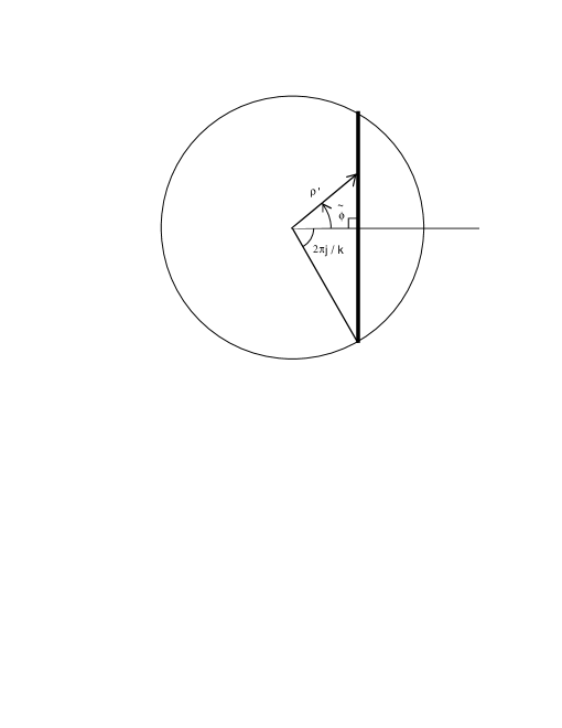
Figure 1: The shape of a D1-brane for fixed $j$ described by (48).

The boundary condition for open strings (47) obtained from the vectorially gauged WZW model can be verified from the scattering amplitude between the boundary states and closed string states. The action (45) indicates that the wave functions on the disk $(\rho^{\prime},\tilde{\phi})$ are $SU(2)$ wave functions that are invariant under translations of $\phi$. So, the wave functions of the parafermion theory are 

$$\Psi_{j,m}(\theta,\tilde{\phi}) \ =\ \langle j,m|g|j,m\rangle\ =\ e^{i2m\tilde{\phi}}\langle j,m|e^{i2\theta J^{1}}|j,m\rangle$$ (50)

$$\ =\ \frac{1}{\sqrt{2j+1}}\langle\theta,\tilde{\phi}|g|j,m,m\rangle_{PF}$$

where the $|j,m\rangle$ are a basis for the spin $j$ representation of $SU(2)$.

The Cardy boundary states for A-branes are [1]

$$|A,\hat{j},\hat{n}\rangle_{C}\ =\ \sum_{(j,n)\in PF(k)}\frac{S_{\hat{j}\hat{n}}^{PFjn}}{\sqrt{S_{00}^{PFjn}}}|A,j,n\rangle\rangle\ .$$ (51)

The scattering amplitude between A-brane boundary states and closed string states is [16][1]

$${}_{C}{\langle}A,\hat{j},\hat{m}|\theta,\tilde{\phi}\rangle \sim \sum_{j}S_{\hat{j},j}e^{\frac{i4\pi m\hat{m}}{k}}\Psi_{j,m}(\theta,\tilde{\phi})^{*}=\sum_{j}\sin\Big{[}\frac{2\hat{j}\pi}{k+2}(2j+1)\Big{]}$$ (52)

$$\cdot\Big{[}\sum_{m=-j}^{j}\langle j,m|e^{i2(\tilde{\phi}-\frac{2\pi\hat{m}}{k})J^{3}}e^{i2\theta J^{1}}|j,m\rangle\Big{]}^{*}$$

where we have assumed $k\gg 1$.

To calculate ${}_{C}{\langle}A,\hat{j},\hat{m}=0|\theta,\tilde{\phi}\rangle$, we exploit the relation

$$\sum_{m=-j}^{j}\langle j,m|e^{i2\tilde{\phi}J^{3}}e^{i2\theta J^{1}}|j,m\rangle\ =\ \frac{\sin(2j+1)\tilde{\psi}}{\sin\tilde{\psi}}$$ (53)

with

$$\cos\tilde{\psi}=\cos\theta\cos\tilde{\phi}\ .$$ (54)

Inserting (53) and (54) into (52), we get

$${}_{C}{\langle}A,\hat{j},\hat{m}=0|\theta,\tilde{\phi}\rangle\ \sim\ \delta(\tilde{\psi}-\frac{2\hat{j}\pi}{k})$$ (55)

Eqs. (54) and (55) show that the shape of an A-brane in the parafermion theory is described by

$$\cos\frac{2\hat{j}\pi}{k}=\cos\theta\cos\tilde{\phi}\ \ .$$ (56)

This agrees with (47), obtained above from the vectorially gauged WZW model for open strings.

Since $0\leq j\leq\frac{k}{2}$, the boundary condition (48) shows that the $k-1$ spherical D2-branes in the $SU(2)$ group manifold turn into $k-1$ D1-branes. The two original D0-branes in $SU(2)$ are projected to D0-branes in the disk $(\rho^{\prime},\tilde{\phi})$. All this is illustrated in Figure 2.

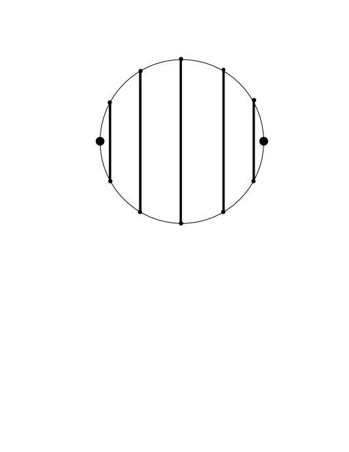
Figure 2: In the level $k(=6)$ case, there are $k-1(=5)$ straight D1-branes and two D0-branes on the disk.

The vectorially gauged WZW action for open strings is invariant under the transformation $g\rightarrow g{\underline{l}}^{-1}$ where the fixed $U(1)$ group element ${\underline{l}}$ is not quantized, but the boundary condition changes. In the parametrization (36), this $U(1)$ transformation is realized as $\phi\rightarrow\phi-\beta$, $\tilde{\phi}\rightarrow\tilde{\phi}+\beta$. To match the result in $\sigma$-model of open strings with that in CFT, Eq.(52) shows that the boundary condition should be modified as

$$\cos\psi_{j}=\cos\theta\cos(\tilde{\phi}-\frac{n\pi}{k})$$ (57)

where $-k+1\leq n\leq k$, that is, $U(1)$ symmetry is broken to $\mbox{$ZZ$}_{2k}$ symmetry. From CFT points of view, when the pairs subject to a constraint $2j+n=0$ mod 2, then half of the number of $n$ is eliminated, and we are left with $\mbox{$ZZ$}_{k}$ symmetry. Eq.(57) shows that when $j=0$ there are $k$ D0-branes at one of the $k$ special points around the disk, and $\left(k\atop 2\right)$ D1-brane states with $j=\frac{1}{2},1,\ldots,\frac{1}{2}[\frac{k}{2}]$ which stretch between two of the special points around the disk separated by $2j$ segments as shown in Figure 3.

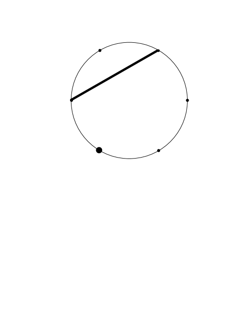
Figure 3: The geometry of A-branes for fixed $j$ in the $k=6$ case. The points marked around the boundary disk indicate the possible D0-branes.

From the surviving boundary condition (48) and the $\mbox{$ZZ$}_{k}$ symmetry, we have recovered the geometry of A-branes uncovered in [1]. There this picture was conjectured, mainly from CFT. The geometrical interpretation of A-branes in the $SU(2)/U(1)$ coset model is that the spherical D2-branes on the $SU(2)$ group manifold are projected to the disk $(\rho^{\prime},\tilde{\phi})$, and the resulting shape is a straight line.

4 B-branes and axial-vector duality

Since there is a $\mbox{$ZZ$}_{k}$ symmetry in the parafermion theory, it was argued in [1] that the level $k$ $SU(2)/U(1)$ coset model is equivalent to its $\mbox{$ZZ$}_{k}$ orbifold. A-branes in the orbifold theory are constructed from A-branes in its covering theory by adding the images under $\mbox{$ZZ$}_{k}$ so that the configuration is $\mbox{$ZZ$}_{k}$ invariant. Then T-duality maps these branes to B-branes in the original theory.

In the orbifold, the range of values of the angle $\tilde{\phi}$ is changed to $[0,\frac{2\pi}{k}]$. If we introduce a new angle $\hat{\phi}=k\tilde{\phi}$ with $\hat{\phi}\rightarrow\hat{\phi}+2\pi$, then (45),(46), then (49) can be rewritten as

$$S^{SU(2)/U(1)_{V}}=\int d^{2}z\Big{(}\frac{k}{1-\rho^{\prime 2}}\partial_{z}{\rho^{\prime}}\,\partial_{\bar{z}}{\rho^{\prime}}+\frac{\rho^{\prime 2}}{k(1-\rho^{\prime 2})}\partial_{z}\hat{\phi}\,\partial_{\bar{z}}\hat{\phi}\Big{)}$$ (58)

$$g_{s}(\rho^{\prime})=g_{s}(0)(1-\rho^{\prime 2})^{-\frac{1}{2}}$$ (59)

$$\left(\hat{\phi}-k\arccos\sqrt{\frac{1-\rho^{2}_{j}}{1-\rho^{2}}}\,\right)_{\partial\Sigma}=0$$ (60)

We now perform a T-duality transformation for open strings [23] along the circle $S^{1}$ parametrized by $\hat{\phi}$. In the dual theory, strings end on the hypersurface defined by setting the coordinate in the direction of the Killing vector equal to the corresponding component of the gauge potential [23]. We find the action

$$S^{dual}=k\int d^{2}z\,\frac{1}{1-\rho^{2}}\Big{(}\partial_{z}{\rho}\,\partial_{\bar{z}}{\rho}+\rho^{2}\partial_{z}\phi\,\partial_{\bar{z}}\phi\Big{)}+\int_{\partial\Sigma}a$$ (61)

with

$$g_{s}(\rho)=\sqrt{k}g_{s}(0)(1-\rho^{2})^{-\frac{1}{2}}$$ (62)

and

$$a=-k\arccos\sqrt{\frac{1-\rho^{2}_{j}}{1-\rho^{2}}}\,d\phi$$ (63)

where $\phi$ is the coordinate dual to $\hat{\phi}$.

By the variation of the action (61), the boundary condition is

$$\left(\partial_{\sigma}\rho+\sqrt{1-\rho^{2}_{j}}\frac{\rho}{\sqrt{\rho^{2}_{j}-\rho^{2}}}\partial_{\tau}\phi\right)_{\sigma=0,\pi} = 0$$

$$\left(\partial_{\sigma}\phi-\sqrt{1-\rho^{2}_{j}}\frac{1}{\rho\sqrt{\rho^{2}_{j}-\rho^{2}}}\partial_{\tau}\rho\right)_{\sigma=0,\pi} = 0$$ (64)

where the coordinates are related by $\partial_{z}=\partial_{\tau}-\partial_{\sigma},\ \partial_{\bar{z}}=\partial_{\tau}+\partial_{\sigma}$. Eq.(64) describes a D2-brane disk. The gauge field strength on this D2-brane is

$$F\ =\ da\ =\ k\frac{\rho}{1-\rho^{2}}\sqrt{\frac{1-\rho^{2}_{j}}{\rho^{2}_{j}-\rho^{2}}}\,d\rho\wedge d\phi\ .$$ (65)

This shows that the D2-brane disk should have radius $\rho=\rho_{j}=\sin\frac{2j\pi}{k}$ and be centered, as illustrated in Figure 4.

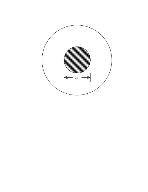
Figure 4: The shape of D2-branes with radius $\rho_{j}=\sin\frac{2j\pi}{k}$.

Because of this nonzero gauge field strength, the B-branes are stable and cannot decay by shrinking or displacing off the center of the disk. This was shown in [1], where the B-branes were described by an effective theory, and the classical equations for a disk D2-brane with a gauge field strength $F$ were considered. A fixed flux of $F$ on the B-brane was assumed and its value was calculated by minimizing the Dirac-Born-Infeld action. The $F$ they obtained by their minimization procedure is exactly the same as that in (65). However, in the above approach, such minimization is unnecessary. The gauge field strength $F$ on the D2-brane is obtained more directly – from the gauged WZW model, by first gauging away the vector $U(1)$ subgroup, then orbifolding and transforming to the T-dual theory.

The mass of the B-branes can be calculated from the Dirac-Born-Infeld action

$$M_{D2}=\int g_{s}^{-1}(\rho)\sqrt{-det(G_{\alpha\beta}+F_{\alpha\beta})}=\frac{2\pi\sqrt{k}}{g_{s}(0)}\sin\frac{2j\pi}{k}\ .$$ (66)

For large $k$ this mass is proportional to

$$M_{j}=\frac{1}{g_{s}(0)\sqrt{k(k+2)}}\sin\frac{(2j+1)\pi}{k}\ .$$ (67)

Thus the mass derived from the $\sigma$-model for open strings matches that found from CFT.

Consider the axially gauged WZW action for open strings (24). If we insert (42) and (36) into (24), we get

$$S^{G/U(1)_{A}}\ =\ k\int d^{2}z\,\Big{(}\partial_{z}\theta\,\partial_{\bar{z}}\theta+\tan^{2}\theta\,\partial_{z}\phi\,\partial_{\bar{z}}\phi\qquad\qquad\qquad$$

$$\qquad\qquad\qquad+\cos^{2}\theta(A+\partial_{z}\tilde{\phi}+\tan^{2}\theta\,\partial_{z}\phi)(\bar{A}+\partial_{\bar{z}}\tilde{\phi}-\tan^{2}\theta\,\partial_{\bar{z}}\phi)\Big{)}$$

$$\qquad\qquad\qquad-k\oint_{\partial\Sigma}\arccos\sqrt{\frac{1-\rho^{2}_{j}}{1-\rho^{2}}}\,d\phi\ .$$ (68)

Here we have omitted an irrelevant overall factor, and chosen the NS B-field as $B=-2\sin^{2}\theta d\phi\wedge d\tilde{\phi}$. Integrating the gauge fields $A$ and $\bar{A}$ out, we obtain the $\sigma$-model for B-branes described by (61)-(63). This shows that the B-branes can be realized in the gauged WZW action with axial $U(1)$ gauge subgroup.

In [1], the operator $\exp(i\pi\tilde{J}_{0}^{1})$ was exploited to define B-type Ishibashi states in the parafermion theory:

$$(1\otimes e^{i\pi\tilde{J}_{0}^{1}})|j\rangle\rangle^{SU(2)}=\sum_{r=0}^{2k-1}|Bj,r,-r\rangle\rangle^{PF}\otimes|B,r,-r\rangle\rangle^{U(1)_{k}}$$ (69)

The A-type Ishibashi states in the $SU(2)$ group manifold satisfy the boundary condition

$$(J_{n}+R\tilde{J}_{-n})|j\rangle\rangle^{SU(2)}\ =\ 0$$ (70)

with $RJ^{a}=J^{a}$, for all $a$. The Cardy boundary states constructed from these maximally symmetric Ishibashi states therefore describe spherical D2-branes. Since

$$e^{i\pi\tilde{J}_{0}^{1}}\tilde{J}_{n}^{2}e^{-i\pi\tilde{J}_{0}^{1}}=-\tilde{J}_{n}^{2},\ \ e^{i\pi\tilde{J}_{0}^{1}}\tilde{J}_{n}^{3}e^{-i\pi\tilde{J}_{0}^{1}}=-\tilde{J}_{n}^{3}$$ (71)

we have

$$(J_{n}+R^{\prime}\tilde{J}_{-n})(1\otimes e^{i\pi\tilde{J}_{0}^{1}})|j\rangle\rangle^{SU(2)}=0$$ (72)

with $R^{\prime}J^{a}=(-1)^{\delta_{a,1}}J^{a}$. Then the boundary states $(1\otimes e^{i\pi\tilde{J}_{0}^{1}})|j\rangle\rangle^{SU(2)}$ are also maximally symmetric. The corresponding Cardy boundary states describe another set of spherical D2-branes obtainable by a global rotation of the first set. Thus the geometrical interpretation of B-branes is that the spherical D2-branes in the $SU(2)$ group manifold are projected to the $(\rho,\phi)$ disk, and their shape is a centered disk with the radius $\rho=\rho_{j}=\sin\frac{2j\pi}{k}$. The quantized gauge field strengths in the original spherical D2-branes of the $SU(2)$ parent theory are inherited by these disk B-branes, making them stable.

5 Summary and Discussion

We have constructed D-branes in a left-right asymmetrically gauged WZW model for open strings. The asymmetry was restricted to the type induced from different embeddings of the gauge subgroup acting on the left and right of the group-valued field $g$. Boundary conditions were written for $g$ that preserve this symmetry. For a subgroup $H\cong U(1)$, the axially gauged WZW action was found, and the vectorially gauged WZW action was then reproduced by implementing T-duality. We find that the boundary condition for the T-dual coordinate is $\tilde{X}(\tau)=0$, while for the original $U(1)$ coordinate $X$ it is $e^{iX(\tau)T^{0}}=s\tilde{s}^{-1}(\tau)$. The axial-vector duality in the open string case is realized with such a change of the boundary condition. We conclude that the axially gauged WZW model is T-dual to a $\mbox{$ZZ$}_{k}$ orbifold of the vectorially gauged WZW model. This is an example of an axial-vector duality in open strings.

From the $SU(2)/U(1)$ coset model, described by the vectorially gauged WZW model, we found a vanishing gauge field on D-branes. Since the geometry of the disk is conformally flat and the gauge field on D-branes vanishes, there is a boundary condition in the $SU(2)$ parent theory that remains intact. From this surviving boundary condition for D-branes in the $SU(2)/U(1)$ coset model, we have shown that the shape of an A-brane is a straight line.

This observation was supported by scattering amplitudes. In the parafermion theory there is a global $U(1)$ symmetry, but the consistency of the gauged WZW model for open strings does not demand that the $U(1)$ parameter be quantized. Matching the results of the $\sigma$-model and CFT, the scattering amplitudes between boundary states for A-branes and closed string states indicate that the $U(1)$ symmetry has to be broken to a $\mbox{$ZZ$}_{2k}$ symmetry, i.e., with $2k$ end-points on the disk boundary. The group-theoretical selection rule eliminates half of the interval endpoints, and we are left with a $\mbox{$ZZ$}_{k}$ symmetry.

Using this $\mbox{$ZZ$}_{k}$ symmetry, we have constructed the $\mbox{$ZZ$}_{k}$ orbifold so that we can implement T-duality. Orbifolding and then T-dualizing maps the original conformally flat disk to another conformally flat disk. The gauge field on B-branes was obtained from the boundary condition for A-branes. From the resulting $\sigma$-model, we derived the boundary condition for B-branes, showing that they are centered disks. The obtained gauge field strengths stabilize the B-branes, i.e., they prevent B-brane decay by shrinking or displacing off the center. As the $\sigma$-model action for B-branes can be recast into the axially gauged WZW action, we conclude that an axial-vector duality exists in the $SU(2)/U(1)$ coset model for open strings.

Finally, let us comment on certain differences between our results and those of [1]. There the shape of A-branes was discussed mainly from the CFT point of view. Target space arguments were based on consideration of $\sigma$-models without boundaries only. In addition, while the field theory realization of the $SU(2)/U(1)$ coset model is the vectorially gauged WZW model, the axial coset was used to describe the geometry of its branes. Consequently, the shape of an A-brane was conjectured in [1] to be a straight line in the disk $(\rho,\phi)$. In our case, we started with the vectorially gauged WZW action for open string. From the surviving boundary condition (48) and the $\mbox{$ZZ$}_{k}$ symmetry, we showed explicitly that the shape of an A-brane in the $SU(2)/U(1)$ coset model is a straight line, obtained by projecting the spherical D2-branes in the $SU(2)$ parent theory to the disk $(\rho^{\prime},\tilde{\phi})$.

Also, the authors of [1] found that when the gauge field strength $F$ on B-branes is put in by hand, the B-branes will be stable. A fixed flux of $F$ on the B-brane was assumed and its value was calculated by minimizing the Dirac-Born-Infeld action. In our approach, however, such minimization is unnecessary. The gauge field strength $F$ on the B-brane is obtained more directly – from the gauged WZW model, by first gauging away the vector $U(1)$ subgroup, then orbifolding and transforming to the T-dual theory. The quantized gauge field strengths in the original spherical D2-branes of the $SU(2)$ parent theory are inherited by these disk B-branes, making them stable.

References

- [1] J. Maldacena, G. Moore, N. Seiberg, Geometrical interpretation of D-branes in gauged WZW models, JHEP 0107 (2001) 046, hep-th/0105038.
- [2] K. Gawedzki, Boundary WZW, , and CS theories, hep-th/0108044.
- [3] S. Elitzur, G. Sarkissian, D-Branes on a gauged WZW model, Nucl. Phys. B 625 (2002) 166-178, hep-th/0108142.
- [4] S. Parvizi, Effective action for D-branes on gauged WZW model, Phys. Lett. B 520 (2001) 367, hep-th/0108095.
- [5] S. Fredenhagen, V. Schomerus, D-branes in coset models, hep-th/0111189.
- [6] H. Ishikawa, Boundary states in coset conformal field theories, hep-th/0111230.
- [7] T. Kubota, J. Rasmussen, M.A. Walton, J.-G. Zhou, Maximally symmetric D-branes in gauged WZW models, Phys. Lett. B 544 (2002) 192, hep-th/0112078.
- [8] Y. Hikida, Orientifold of WZW model, hep-th/0201175.
- [9] K. Gawedzki, A. Kupiainen, conformal field theory from gauged WZW model, Phys. Lett. B 215 (1988) 119; Coset construction from functional integrals, Nucl. Phys. B 320 (1989) 625.
- [10] D. Karabali, Q. Park, H.J. Schnitzer, Z. Yang, A GKO construction based on a path integral formulation of gauged Wess-Zumino-Witten action, Phys. Lett. B 216 (1989) 307; D. Karabali, H.J. Schnitzer, BRST quantization of the gauged WZW action and coset conformal field theories, Nucl. Phys. B 329 (1990) 649.
- [11] R. Dijkgraaf, H. Verlinde, E. Verlinde, String propagation in a black hole geometry, Nucl. Phys. B 371 (1992) 269.
- [12] E. Kiritsis, Duality in gauged WZW model, Mod. Phys. Lett. A 6 (1991) 2871.
- [13] E. Kiritsis, Exact duality symmetries in CFT and string theory, Nucl. Phys. B 405 (1993) 109, hep-th/9302033.
- [14] E. Alvarez, L. Alvarez-Gaume, J. Barbon, Y. Lozano, Some global aspects of duality in string theory, Nucl. Phys. B 415 (1994) 71, hep-th/9309039.
- [15] A. Giveon, E. Kiritsis, Axial vector duality as a gauge symmetry and topology change in string theory, Nucl. Phys. B 411 (1994) 487, hep-th/9303016.
- [16] G. Felder, J. Fröhlich, J. Fuchs, C. Schweigert, The geometry of WZW branes, J. Geom. Phys. 34 (2000) 162, hep-th/9909030.
- [17] A.Y. Alekseev, V. Schomerus, D-branes in the WZW model, Phys. Rev. D 60 (1999) 061901, hep-th/9812193.
- [18] I. Bars, K. Sfetsos, Generalized duality and singular strings in higher dimensions, Mod. Phys. Lett. A 7 (1992) 1091, hep-th/9110054.
- [19] A.A. Tseytlin, Effective action of gauged WZNW model and exact string solutions, Nucl. Phys. B 399 (1993) 601, hep-th/9301015.
- [20] E. Witten, On holomorphic factorization of WZW and coset models, Comm. Math. Phys. 144 (1992) 189.
- [21] K. Sfetsos, A.A. Tseytlin, Chiral gauged WZNW models and heterotic string backgrounds, Nucl. Phys. B 415 (1994) 116, hep-th/9308018.
- [22] E. Alvarez, J. Barbon, J. Borlaf, T-duality for open strings, Nucl. Phys. B 479 (1996) 218, hep-th/9603089.
- [23] H. Dorn, H.J. Otto, On T-duality for open strings in general abelian and nonabelian gauge field backgrounds, Phys. Lett. B 381 (1996) 81 hep-th/9603186.
- [24] J. Borlaf, Y. Lozano, Aspects of T-duality in open strings, Nucl. Phys. B 480 (1996) 239, hep-th/9607051.
- [25] S. Forste, D-branes on a deformation of , hep-th/0112193.
- [26] J. Fuchs, P. Kaste, W.Lerche, C. Lutken, C. Schweigert, J. Walcher, Boundary Fixed Points, Enhanced Gauge Symmetry and Singular Bundles on K3, Nucl. Phys. B598 (2001) 57, hep-th/0007145; J. Fuchs, L.R. Huiszoon, A.N. Schellekens, C. Schweigert, J. Walcher, Boundaries, crosscaps and simple currents, Phys. Lett. B495 (2000) 427, hep-th/0007174.
- [27] J.-G. Zhou, Page charge of D-branes and its behavior in topologically nontrivial B-fields, Phys. Rev. D 64 (2001) 066003, hep-th/0105106; T. Kubota, J.-G. Zhou, RR charges of D2-branes in group manifold and Hanany-Witten effect, JHEP 0012 (2000) 030, hep-th/0010170.
- [28] G. Sarkissian, Non-maximally symmetric D-branes on group manifold in the Lagrangian approach, hep-th/0205097.