Perturbative Evaluation of the Effective Action for a Self-Interacting Conformal Field on a Manifold with Boundary

Abstract.

In a series of three projects a new technique which allows for higher-loop renormalisation on a manifold with boundary has been developed and used in order to assess the effects of the boundary on the dynamical behaviour of the theory. Commencing with a conceptual approach to the theoretical underpinnings of the, underlying, spherical formulation of Euclidean Quantum Field Theory this overview presents an outline of the stated technique’s conceptual development, mathematical formalism and physical significance.

I. Introduction

The investigation of the effects generated on the dynamical behaviour of quantised matter fields by the presence of a boundary in the background geometry is an issue of central importance in Euclidean Quantum Gravity. This issue arises naturally in the context of any evaluation of radiative corrections to a semi-classical tunnelling geometry and has been studied at one-loop level through use of heat kernel and functional techniques. These methods were subsequently extended in the presence of matter couplings. Despite their success, however, such techniques have limited significance past one-loop order. Not only are explicit calculations of higher-order radiative effects far more reliable for the qualitative assessment of the theory’s dynamical behaviour under conformal rescalings of the metric but they are, in addition, explicitly indicative of boundary related effects on that behaviour. Such higher-order calculations necessarily rely on diagrammatic techniques on a manifold with boundary. Fundamental in such a calculational context is the evaluation of the contribution which the boundary of the manifold has to the relativistic propagator of the relevant quantised matter field coupled to the manifold’s semi-classical background geometry. It would be instructive, in this respect, to initiate an approach to such a higher loop-order renormalisation on a manifold with boundary by outlining the considerations which eventuated in the ”background field” method, that approach to metric quantisation which is predicated on a fixed geometrical background.

The analysis relevant to the background field method can most easily be exemplified in the case of a massless scalar field minimally coupled to the background geometry. In the case of flat Euclidean space - defined by the analytical extension which eventuates in the replacement of $x_{0}$ by $-ix_{0}$ - the generating functional relevant to the massless scalar field $\phi$ coupled to a classical source $J$ is

(1) $$Z[J]=\int D[\phi]e^{-\int d^{4}x[\frac{1}{2}\phi\partial^{2}\phi-J\phi]}$$

which, upon Gaussian integration yields

(2) $$Z[J]=[det(\partial^{2})]^{-\frac{1}{2}}e^{\int d^{4}xd^{4}y[J(x)\Delta(x,y)J(y)]}$$

as a result of which, the scalar propagator of momentum $k$

$$x---------y$$

is

(3) $$\Delta(x,y)=\int\frac{d^{4}k}{(2\pi)^{4}}\frac{e^{ik.(x-y)}}{k^{2}}$$

The generating functional in the presence of gravity with a minimal coupling between the massless scalar field and the background metric $g_{\mu\nu}$, which for the sake of mathematical consistency in the context of the present formalism is taken to have a Euclidean signature, is

(4) $$Z[J]=\int D[\phi]e^{-\int d^{4}x\big{[}\frac{1}{2}\phi[(\frac{1}{\sqrt{g}}\partial_{\mu}g^{\mu\nu}\sqrt{g}\partial_{\nu})g]\phi-J\phi\sqrt{g}\big{]}}$$

where the Riemannian manifold has been assumed, without loss of generality, to have no boundary so as to allow for vanishing surface terms. Again, Gaussian integration results in

(5) $$Z[J]=[det(\frac{1}{\sqrt{g}}\partial_{\mu}g^{\mu\nu}\sqrt{g}\partial_{\nu})g]^{-\frac{1}{2}}e^{\frac{1}{2}\int d^{4}xd^{4}y\big{[}J(x)G(x,y)J(y)\big{]}}$$

which reveals the scalar propagator

(6) $$G(x,y)=<x|\big{[}(\frac{1}{\sqrt{g}}\partial_{\mu}g^{\mu\nu}\sqrt{g}\partial_{\nu})g]^{-1}|y>$$

with $|x>,|y>$ being orthonormal vectors in a suitably defined Hilbert space.

It would appear that the presence of such a propagator on the fixed geometrical background $g_{\mu\nu}$ is consistent and would, for that matter, allow for the evaluation of scalar vacuum effects on condition of a tractable mathematical expression for the inverse to the associated metric-dependent kernel. Such an appearance, however, is physically irrelevant. If the coupling between the scalar field and the background geometry is strong enough for the renormalisation group behaviour of the theory to justify the second quantisation of the former then, inevitably, the non-linear character of gravity in the context of the equivalence principle will render gravity, itself, just as much subject to second quantisation with the same degree of physical necessity [1]. The quantisation of gravity enters, for that matter, non-trivially at all scales, a fact which necessitates a consistent approach at least at the level of the quantisation of the background metric $g_{\mu\nu}$. In the absence of a consistent quantum theory of gravity it would appear reasonable, in this respect, to pursue a linearised approach to second quantisation by quantising linear local perturbations $h_{\mu\nu}$ of the background metric $g^{c}_{\mu\nu}$ successfully implemented through

(7) $$g_{\mu\nu}=g^{c}_{\mu\nu}+h_{\mu\nu}$$

so as to allow for $h_{\mu\nu}$ to be treated as a null fluid in the stress tensor [2].

In the spirit of the background field approach to metric quantisation as outlined above the quantised linear perturbations $h_{\mu\nu}$ represent the graviton, the quantum of the metric field propagating on the fixed background $g^{c}_{\mu\nu}$. Naturally, in such an approach the weakness of the gravitational coupling $G$ with respect to any other matter-field couplings at length scales well above the Planck scale allows for a consistent perturbative expansion with respect to the latter while keeping the former at the second-quantised zero order. The evaluation of such a perturbative expansion at high orders is predicated on a concrete mathematical expression for the matter-field propagator on $g^{c}_{\mu\nu}$. Such an issue, is in general, non-trivial. Specifically, the inverse to the kernel for the scalar propagator in (6) does not readily admit a closed expression in a general space-time. The only consistent approach in the content of the background field method is its treatment as a perturbative expansion through (7). The relevant diagrammatic representation involves both graviton-contributions which the scalar propagator on the background geometry of $g^{c}_{\mu\nu}$ receives to all orders

Figure 1. Graviton contributions to the scalar propagator

and scalar-contributions which the graviton propagator on the same background receives to all orders.

The other dynamical aspect which (5) involves, in addition to that of the two propagators, stems from the associated determinant. Contrary to the Minkowski-space case expressed in (2), the metric-dependent determinant in (5) contributes non-trivially to the vacuum-to-vacuum amplitude expressed by $Z[J]$. It has to be subjected, for that matter, to the same perturbative expansion through (7), an operation which is consistently accomplished through the exponentiation

(8) $$e^{-\frac{1}{2}Trln(\frac{1}{\sqrt{g}}\partial_{\mu}g^{\mu\nu}\sqrt{g}\partial_{\nu})g}$$

The trace in the exponentiated determinant results effectively in $x\rightarrow y$ and generates, for that matter, a new diagrammatic representation with each of the previous scalar propagators closing upon itself

Figure 2. One-loop contributions to the effective action

as well as with each of the graviton propagators undergoing the same process.

The diagrammatic expansions for the scalar and graviton propagators as well as for that of the one-loop effective action correspond to representations derived through adiabatic expansions in Riemann normal coordinates and heat kernel techniques [3]. It is evident that, the necessary for perturbation, closed expression for such expansions is unattainable unless the relevant space-time is characterised by a high degree of symmetry. The natural candidate for such a space-time is the only maximally symmetric curved manifold, the de Sitter space. The $n$-dimensional de Sitter space can be represented as a hyperboloid

(9) $$z_{0}^{2}-\sum_{i=1}^{n}z_{i}^{2}=-a^{2}$$

embedded in a $n+1$-dimensional Minkowski space with metric

(10) $$ds^{2}=dz_{0}^{2}-\sum_{i=1}^{n}dz_{i}^{2}$$

The Euclidean analogue of this space is a $n$-dimensional sphere $S_{n}$ of radius $a$

(11) $$\sum_{i=1}^{n+1}z_{i}^{2}=a^{2}$$

embedded in a $n+1$-dimensional Euclidean space. Since de Sitter space is conformally equivalent to Minkowski space the action for a massless scalar field conformally coupled to the background geometry of $S_{n}$ can readily be obtained by a conformal transformation of the corresponding exponentiated action featured in (1), in flat Euclidean space [4]

(12) $$S[\Phi]=\int d^{n}\sigma\big{[}\frac{1}{2}\frac{1}{2a^{2}}\Phi(L^{2}-\frac{n(n-2)}{2})\Phi-\frac{\lambda}{\Gamma(p+1)}\Phi^{p}\big{]}$$

with $d^{n}\sigma=a^{n}\Omega_{n+1}$ being the volume element of the embedded $S_{n}$, with $p=\frac{2n}{n-2}$ and with

(13) $$L_{ab}=\eta_{a}\frac{\partial}{\partial\eta_{b}}-\eta_{b}\frac{\partial}{\partial\eta_{a}}$$

being the generator of rotations on $S_{n}$ defined in terms of the embedding vector $\eta$. The formal equivalence between the spherically formulated scalar action obtained through the stated conformal transformation and the conformal scalar action defined directly on $S_{n}$ has been shown [5].

It is evident that the closed expression which the kernel associated with the quadratic expression for the scalar field in (12) admits results, upon Gaussian integration over its exponentiated expression which replaces that in (4), in an exact expression for the scalar propagator $D(\eta,\eta^{\prime})$ in (Euclidean) de Sitter space. Such an expression represents, in effect, an exact result for the formal summation of the graviton contributions to the scalar propagator

Figure 3. Exact propagator as a result of maximal symmetry

and is given by the elementary Haddamard function for propagation between the space-time points $\eta$ and $\eta^{\prime}$ on $S_{4}$ [4]

(14) $$D(\eta,\eta^{\prime})=-\frac{1}{4{\pi}^{2}}\frac{1}{|\eta-\eta^{\prime}|^{2}}$$

The preceding analysis, effectively, reveals how maximal symmetry renders the evaluation of higher-loop order vacuum effects and renormalisation tractable on a curved manifold. For example, the infinite series of diagrams in the case of a three-loop vacuum diagram effected by the presence of a $\lambda\phi^{4}$ self-interaction in a general space-time amounts on $S_{4}$ to an exact expression for a three-loop diagram derived from the scalar propagator $D(\eta,\eta^{\prime})$

Figure 4. Higher-loop evaluation attained by maximal symmetry

In outlining the merit which maximal symmetry has for higher-loop renormalisation the preceding analysis calls into question the possibility of any extension of the concommitant spherical formulation to the physically important case of the spherical cap $C_{4}$. The $C_{n}$ is the n-dimensional Riemannian manifold of constant positive curvature embedded in an $n+1$-dimensional Euclidean space and bounded by a $n-1$-dimensional sphere of positive extrinsic curvature $K$ (diverging normals). From the outset, such a geometric context is impervious to a direct application of the spherical formulation of a quantum field theory in four dimensions and, yet, suggestive of it. Specifically, the presence of a boundary in the manifold of constant positive curvature dispenses altogether with maximal symmetry. The remaining symmetry falls short of meeting the demand of expunging the theory of the mathematical complications hitherto discussed. It would be instructive, in this respect, to outline the fundamental differences which the direct application of the spherical formulation entails in the case of a massless conformal field coupled to the background geometry of $S_{n}$ and to that of $C_{n}$ with a Dirichlet condition of a vanishing value $\Phi_{\partial C}=0$ on the boundary. The unbounded Laplace operator $M$ defined on $S_{n}$ being the kernel in the quadratic expression for the spherical action in (12)

(15) $$M=\frac{1}{2}\frac{1}{2a^{2}}\big{[}L^{2}-\frac{n(n-2)}{2})\Phi-\frac{\lambda}{\Gamma(p+1)}\big{]}$$

is conformally related to the corresponding d’Alambertian $\partial^{2}$ in flat space-time and admits a complete set of eigenfunctions

(16) $$MY_{\alpha}^{N}(\eta)=\lambda_{N}Y_{\alpha}^{N}(\eta)$$

The latter are the spherical harmonics $Y_{\alpha}^{N}(\eta)$ on $S_{n}$ [4]. They are characterised by an integer degree $N$ which is physically associated with the angular momentum flowing through the relevant propagator. In effect, the Green function $D(\eta,\eta^{\prime})$ associated with $M$

(17) $$MD(\eta,\eta^{\prime})=\delta^{(n)}(\eta,\eta^{\prime})$$

admits an expansion in terms of $Y_{\alpha}^{N}(\eta)$

(18) $$D(\eta,\eta^{\prime})=\sum_{N=0}^{\infty}\sum_{\alpha=0}^{N}\frac{1}{\lambda_{N}}Y_{\alpha}^{N}(\eta)Y_{\alpha}^{N}(\eta^{\prime})$$

which renders the spherical formulation a concrete mathematical content in configuration space primarily through the - fundamental to perturbative calculations - formula

(19) $$[(\eta-\eta^{\prime})^{2}]^{\nu}=\sum_{N=0}^{\infty}\sum_{\alpha=0}^{N}\frac{(2a)^{2\nu+n}{\pi}^{\frac{n}{2}}\Gamma(\nu+\frac{n}{2})\Gamma(N-\nu)}{\Gamma(N+n+\nu)\Gamma(-\nu)}Y_{\alpha}^{N}({\eta})Y_{\alpha}^{N}({\eta}^{\prime})$$

In light of these mathematical underpinnings relevant to the spherical formulation in the stated case on $S_{n}$ it becomes evident that any attempt for a direct application of the same formulation on $C_{n}$ fails. Specifically, the action for the conformal scalar field although mathematically identical to (12) generates an additional boundary term in the Einstein-Hilbert action $S_{EH}$ involving the extrinsic curvature and the metric $h_{ij}$ induced on the boundary with the stated Dirichlet condition. In effect, the action $S$ for the theory on $C_{n}$ is the additive result of (12) and the gravitational action

(20) $$S=S[\Phi]+S_{EH}$$

with $S_{EH}$ being for $n=4$ [6]

(21) $$S_{EH}=-\frac{1}{16\pi}\frac{1}{G}\int_{C}d^{4}\sigma(R-2\Lambda)+\int_{\partial C}d^{3}x\sqrt{h}K\Phi^{2}$$

As stated, this action is invariant under the set of conformal rescalings of the metric

(22) $$g_{\mu\nu}\rightarrow\Omega^{2}(x)g_{\mu\nu};~{}~{}~{}\Phi\rightarrow\Omega^{1-\frac{n}{2}}\Phi$$

This mathematical context reveals that, although the mathematical expression of the bounded spherical Laplace operator $M_{c}$ on $C_{n}$ remains the same as that of $M$, its different domain generated by the presence of the boundary alters non-trivially the spectrum of eigenvalues thereby generating non-integer degrees $N$. In effect, the $n$-dimensional spherical harmonics $Y_{\alpha}^{N}(\eta)$, although still eigenfunctions of $M_{c}$, no longer form a complete set. For that matter, configuration-space computations on $C_{n}$ are substantially intractable as a result of the absence of the pivotal relation (19) [6]. Moreover, the emergence of fractional degrees would tend to obscure the physical interpretation of any results attained by perturbative calculations. The presence of a boundary is, on the evidence, incompatible with a direct application of the spherical formulation.

It is evident, as a result of the preceding analysis, that the mathematical complications stemming from the presence of the boundary relate directly to the associated eigenvalue problem. It would be desirable, for that matter, to relate the eigenvalue problem for the bounded Laplace operator $M_{c}$ defined on $C_{n}$ to that for the unbounded Laplace operator $M$ on $S_{n}$, the covering manifold of $C_{n}$. The method of images is the simplest expedient to this end and is predicated on the premise that the stated boundary effects which the propagator on $S_{n}$ receives due to $\partial C$ can, themeselves, be treated as equivalent to propagation on $S_{n}$ in a manner which reproduces the boundary condition. In the present case of $\Phi_{\partial C}=0$ the method of images results in [6]

(23) $$D_{c}^{(n)}(\eta,{\eta}^{\prime})=\frac{\Gamma(\frac{n}{2}-1)}{4\pi^{\frac{n}{2}}}\big{[}\frac{1}{|{\eta}-{\eta}^{\prime}|^{n-2}}-\frac{1}{|\frac{a_{{\eta}^{\prime}}}{a_{B}}{\eta}-\frac{a_{B}}{a_{{\eta}^{\prime}}}{\eta}^{\prime}|^{n-2}}\big{]}$$

for the conformal scalar propagator with $a_{{\eta}^{\prime}}$ being the geodesic distance between the cap’s pole and space-time point ${\eta}^{\prime}$ The merit of the method of images is explicit. The fundamental part of the propagator, being identical to (14), signifies propagation on $S_{n}$ whereas the boundary part, which expresses the contributions of $\partial C$ on the fundamental part, can be seen to signify, itself, propagation on $S_{n}$ between the associated space-time points $\frac{a_{{\eta}^{\prime}}}{a_{B}}{\eta}$ and $\frac{a_{B}}{a_{{\eta}^{\prime}}}{\eta}^{\prime}$. In effect, although as stated $D_{c}^{(n)}(\eta,{\eta}^{\prime})$ is impervious to an expansion on the lines of (18) both its fundamental and boundary components admit, in principle, such an expansion. Herein the merit of this technique lies. The spherical formulation emerges independently for both components of the propagator on $C_{n}$. Specifically, the image propagator on $S_{n}$ associated with the boundary component of $D_{c}^{(n)}(\eta,{\eta}^{\prime})$ also admits a desired expansion on the lines of (19). However, although the limit of vanishing geodesic separations at the coincidence limit $\eta\rightarrow\eta^{\prime}$ is, as expected, inherent in the singular component the same limit is unattainable by the boundary component which remains, effectively, always finite - as was mathematically expected from the boundary part of the Green function $D_{c}^{(n)}(\eta,{\eta}^{\prime})$. That, in turn, enforces upon the stated expansion for image propagation the condition of vanishing propagation for geodesic distances smaller than $|\frac{a_{{\eta}^{\prime}}}{a_{B}}{\eta}^{\prime}-\frac{a_{B}}{a_{{\eta}^{\prime}}}{\eta}^{\prime}|$. In effect, the - equivalent to (19) - expansion for image propagation is [7]

(24) $$[|\frac{a_{{\eta}^{\prime}}}{a_{B}}{\eta}-\frac{a_{B}}{a_{{\eta}^{\prime}}}{\eta}^{\prime}|^{2}]^{\nu}=\sum_{N=0}^{N_{0}}\sum_{\alpha=0}^{N}\frac{(2a)^{2\nu+n}{\pi}^{\frac{n}{2}}\Gamma(\nu+\frac{n}{2}+\frac{1}{N_{0}})\Gamma(N-\nu+\frac{1}{N_{0}})}{\Gamma(N+n+\nu+\frac{1}{N_{0}})\Gamma(-\nu)}Y_{\alpha}^{N}({\eta})Y_{\alpha}^{N}({\eta}^{\prime})$$

where use has been made of

(25) $$\sum_{\alpha=0}^{N}Y_{\alpha}^{N}(\frac{a_{{\eta}^{\prime}}}{a_{B}}{\eta})Y_{\alpha}^{N}(\frac{a_{B}}{a_{{\eta}^{\prime}}}{\eta}^{\prime})=\sum_{\alpha=0}^{N}Y_{\alpha}^{N}({\eta})Y_{\alpha}^{N}({\eta}^{\prime})$$

The inverse $\frac{1}{N_{0}}$ of the upper limit related to the cut-off angular momentum $N_{0}$ for image propagation in the arguments of the $\Gamma$ functions ensures the finite character of (24) at $n\rightarrow 4$ and is expected on the grounds that the situation of scalar propagation towards the boundary - that is, that situation characterised by the limit $a_{\eta^{\prime}}\rightarrow a_{B}$ - results in $N_{0}\rightarrow\infty$ at the limit of vanishing geodesic separations $\eta\rightarrow\eta^{\prime}$ in which case, the expansion in (24) is reduced to the exact expansion in (19).

The perturbative evaluations of radiative effects in the configuration space of $C_{4}$ within the mathematical context hitherto outlined necessitate the further specification of the regulating scheme for the concommitant divergences as well as a concrete expression for the necessary integration over the relevant vertices. The definition of the theory in $n$ dimensions is, in fact, suggestive of the technique of dimensional regularisation. The latter manifests all divergences arising from the Feynman integrals at the limit $\eta\rightarrow\eta^{\prime}$ as poles at the dimensional limit of $n\rightarrow 4$ after an analytical extension of the space-time dimensionality $n$. In configuration space any diagramatic calculation on $C_{n}$ involves powers of the propagator $D_{c}^{(n)}(\eta,{\eta}^{\prime})$ and, for that matter, products featuring powers of its fundamental part $|{\eta}-{\eta}^{\prime}|^{2-n}$ and of its boundary part $|\frac{a_{{\eta}^{\prime}}}{a_{B}}{\eta}-\frac{a_{B}}{a_{{\eta}^{\prime}}}{\eta}^{\prime}|^{2-n}$. The former are evaluated through use of (19) and the latter through use of (24). An immediate consequence of (24) is the definite finite character of any power of the boundary part of the propagator. In effect, in the context of dimensional regularisation, all possible divergences at the dimensional limit $n\rightarrow 4$ stem exclusively from the fundamental-part related expansion in (19). This analysis reveals the mathematical origin and physical character of the pole structures in configuration space. These structures arise within the context of integrations of a diagram’s vertices over the relevant manifold’s volume according to the Feynman rules. It can readily be seen from (19) and (24) that such integrations invariably eventuate in the expression $\int_{C}d^{n}{\eta}Y_{\alpha}^{N}(\eta)Y_{\alpha^{\prime}}^{N^{\prime}}(\eta)$. The smaller symmetry associated with the geometry of $C_{n}$ precludes the orthonormality condition which emerges for that integral on $S_{n}$. The result, attained through two successive applications of the divergence theorem, is instead [7]

(26) $$\int_{C}d^{n}{\eta}Y_{\alpha}^{N}(\eta)Y_{\alpha^{\prime}}^{N^{\prime}}(\eta)=Aa^{2}\oint_{\partial C}d^{n-1}{\eta}[KY_{\alpha}^{N}(\eta)Y_{\alpha^{\prime}}^{N^{\prime}}(\eta)+2n_{p}Y_{\alpha^{\prime}}^{N^{\prime}}(\eta)D_{p}Y_{\alpha}^{N}(\eta)]$$

with

(27) $$A=\frac{1}{(N^{\prime}+\frac{n}{2}-1)(N^{\prime}+\frac{n}{2})-(N+\frac{n}{2}-1)(N+\frac{n}{2})};~{}~{}N\neq N^{\prime}$$

and with each surface integral admitting a concrete, although involved, expression in terms of Gegenbauer polynomials. In addition to the radius $a$ of the embedded $\it{C_{n}}$ this expression features, as expected, the extrinsic curvature of $\partial C_{n}$. Evidently, it is exactly this feature of any diagrammatic calculation in configuration space which, as will be explicitly shown, ensures a simultaneous renormalisation of boundary and surface terms in the effective action at any specific loop order. The immediate issue which such simultaneity calls into question is the perturbative generation of surface counterterms in addition to possible novel volume counterterms by vacuum scalar processes in the gravitational effective action on $C_{4}$. As the exclusive source of gravitational counterterms is the zero-point function, an outline of the main aspects of its perturbative evaluation to $O(\hbar^{3})$ would illustrate the highly non-trivial effects of the presence of a boundary on the theory as well as provide an essential demonstration of the merit of the techniques hitherto analysed [8].

On a general, unbounded, four dimensional manifold the bare gravitational action assumes the form [3]

(28) $$S_{g}=\int d^{4}x\sqrt{-g}\big{[}\Lambda_{0}+\kappa_{0}R+a_{0}G+b_{0}H+c_{0}R^{2}\big{]}$$

with

(29) $$G=R_{abcd}R^{abcd}-4R_{ab}R^{ab}+R^{2}~{}~{};~{}~{}H=C_{abcd}C^{abcd}$$

Additional terms are expected in the presence of a boundary.

The first two terms in the perturbative expansion of the zero-point function in powers of $\hbar$ (loop expansion) are diagramatically represented by the graphs of fig.(5).

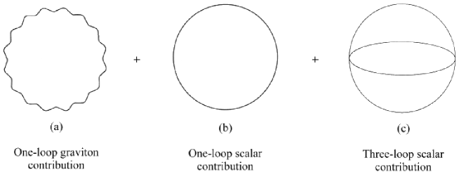
Figure 5. $O(\hbar^{3})$-related contributions to the zero-point function

The “bubble” diagrams in fig.(5a) and fig.(5b) account for the one-loop contribution to the zero-point function of the theory. Their simultaneous presence in any curved space-time is expected on the basis of general theoretical considerations [3], [1]. They are characterised by the absence of interaction vertices and, on power counting grounds, are responsible for the simultaneous one-loop contributions to volume and boundary effective Einstein-Hilbert action on any manifold with boundary. They have been shown to be finite provided that dimensional regularisation is used [6]. In effect, to $O(\hbar^{3})$ the exclusive source of contributions to the bare cosmological constant $\Lambda_{0}$ and the bare gravitational couplings $\kappa_{0},a_{0},b_{0},c_{0}$ in (28) on a general manifold is the diagram in fig.(5c) representing the term

(30) $$I_{c}=\lambda^{2}\int d^{n}{\eta}d^{n}{\eta^{\prime}}[D_{c}^{(n)}(\eta,{\eta}^{\prime})]^{4}$$

On $C_{4}$, the Euclidean de Sitter space, the relation [5]

(31) $$R=\frac{n(n-1)}{a^{2}}$$

effectively reduces (28) to

(32) $$S_{g}=\int d\sigma\big{[}\Lambda_{0}+\kappa_{0}R+c_{0}R^{2}\big{]}$$

In such a context the stated issue of generation of additional counterterms in $S_{g}$ translates to the possibility of additional counterterms generated by the diagram of fig.(5c) on $C_{4}$. A direct replacement of (23) into (30) resolves the double integral with respect to the vertices of the diagram into five such integrals over products of terms of the form (19) and (24). The evaluation of these integrals in the context of (26) and its associated expressions results, at $n\rightarrow 4$ $(\epsilon\rightarrow 0)$ in a substantially involved expression for $I_{c}$ [8]

$$I_{c}=\lambda^{2}\frac{1}{\pi^{4}}\frac{1}{2^{8}}\sum_{N=0}^{\infty}\big{[}\frac{1}{\pi^{2}}\frac{1}{3^{3}}\frac{1}{2^{7}}\frac{(N+2)(N+3)}{(N+1)(N+4)}\big{(}C_{N+1}^{\frac{3}{2}}(cos{\theta_{4}^{0}})\big{)}^{2}+$$

$$\sum_{N^{\prime}=0}^{N^{\prime}_{0}}\frac{1}{[{N^{\prime}}^{2}-N^{2}+3(N^{\prime}-N)]^{2}}[\Gamma(\frac{1}{N^{\prime}_{0}})-\frac{1}{3}\frac{1}{2}\frac{(\Gamma(1+\frac{1}{N^{\prime}_{0}})\Gamma(N^{\prime}+1+\frac{1}{N^{\prime}_{0}})}{\Gamma(N^{\prime}+3+\frac{1}{N^{\prime}_{0}})}(N+1)(N+2)]\times$$

$$3\frac{1}{2^{3}}\frac{1}{\pi^{2}}F^{2}N^{\prime}\big{]}\frac{RK^{2}}{\epsilon}\int_{C}d^{4}{\eta}+$$

$$\lambda^{2}\frac{1}{\pi^{6}}\frac{1}{2^{13}}\sum_{N=0}^{\infty}\sum_{N^{\prime}=0}^{N^{\prime}_{0}}\frac{1}{[{N^{\prime}}^{2}-N^{2}+3(N^{\prime}-N)]^{2}}\times$$

$$\left[\Gamma(\frac{1}{N^{\prime}_{0}})-\frac{1}{3}\frac{1}{2}\frac{(\Gamma(1+\frac{1}{N^{\prime}_{0}})\Gamma(N^{\prime}+1+\frac{1}{N^{\prime}_{0}})}{\Gamma(N^{\prime}+3+\frac{1}{N^{\prime}_{0}})}(N+1)(N+2)\right](BH)^{2}\frac{R^{2}}{\epsilon}\int_{C}d^{4}{\eta}+$$

$$\lambda^{2}\frac{1}{\pi^{6}}\frac{1}{2^{8}}\sum_{N=0}^{\infty}\sum_{N^{\prime}=0}^{N^{\prime}_{0}}\frac{1}{[{N^{\prime}}^{2}-N^{2}+3(N^{\prime}-N)]^{2}}\times$$

$$\left[\Gamma(\frac{1}{N^{\prime}_{0}})-\frac{1}{3}\frac{1}{2}\frac{(\Gamma(1+\frac{1}{N^{\prime}_{0}})\Gamma(N^{\prime}+1+\frac{1}{N^{\prime}_{0}})}{\Gamma(N^{\prime}+3+\frac{1}{N^{\prime}_{0}})}(N+1)(N+2)\right]\times$$

(33) $$(FBH)N^{\prime}\big{(}sin(\theta_{4}^{0})\big{)}^{-3}\frac{RK}{\epsilon}\oint_{\partial C}d^{3}{\eta}$$

The three sectors explicitly featured in this expression are indicative of the theory’s dynamical behaviour on $C_{4}$. The qualitatively new features which the presence of the boundary engenders break the classical conformal invariance and dissociate completely that dynamical behaviour from its corresponding one on $S_{4}$ primarily through the generation of topology-related divergences [8]. There are two volume terms proportional to $RK^{2}$ and $R^{2}$ respectively as well as a surface term proportional to $RK$. The $R^{2}$ term yields a direct contribution to $c_{0}$ in the corresponding sector of (32). However, the $RK^{2}$ term signifies a qualitatively new quantum correction in the bare and, for that matter, effective gravitational action. As $K^{2}$ indicates it is non-trivially generated by $\partial C$. The corresponding $RK$-related sector in the bare gravitational action signifies, indeed, the first surface counterterm generated by vacuum effects on a general manifold with boundary. Moreover, the simultaneous emergence of boundary and surface divergences confirms the theory’s potential for a simoultaneous renormalisation of boundary and surface terms in higher loop-orders.

Acknowledgement

I wish to acknowledge the discrimination, confrontation and contempt with which the “lucky country” received my research effort all these years. My contribution to theoretical research would have never had its present significance without Australia’s mindless rejection.

References

- [1] M. J. Duff, Quantum Gravity II: A Second Oxford Symposium eds. C. J. Isham, R. Penrose, and D. W. Sciama, Oxford: Clarendon (1981)
- [2] B. S. De Witt, Phys. Rev., 160, 1113 (1967); Phys. Rev. 162, 1195 (1967)
- [3] See for example: N. D. Birrell and P. C. W. Davies Quantum Fields in Curved Space, Cambridge University Press (1986) and references therein
- [4] I. Drummond, Nucl. Phys. B 94 115 (1975)
- [5] D. G. C. McKeon and G. Tsoupros Class. Quantum Gravity 11, 73-81 (1994)
- [6] G. Tsoupros, Class. Quantum Gravity 17, 2255 (2000) (e-print Archive: hep-th/0001039
- [7] G. Tsoupros, to appear in Class. Quantum Gravity, (e-print Archive: hep-th/0107019)
- [8] G. Tsoupros, to appear in Class. Quantum Gravity, (e-print Archive: hep-th/0107021)