Analytic continuations of de Sitter thick domain wall solutions
Abstract
We perform some analytic continuations of the de Sitter thick domain wall solutions obtained in our previous paper Sasakura in the system of gravity and a scalar field with an axion-like potential. The obtained new solutions represent anti-de Sitter thick domain walls and cosmology. The anti-de Sitter domain wall solutions are periodic, and correspondingly the cosmological solutions represent cyclic universes. We parameterize the axion-like scalar field potential and determine the parameter regions of each type of solutions.
pacs:
11.27.+d, 04.50.+h, 04.20.JbI Introduction
The solitonic objects in string theory play major roles in the understanding of its non-perturbative properties such as dualities. In string theory the solitons couples necessarily with gravity. In view of the universality of the gravitational interaction, the understanding of the gravitational aspects of solitons may provide deeper understanding of the variety of the dynamics contained in string theory.
The simplest system of solitons and gravity would be domain walls of scalar field theory interacting with gravity. In field theory, domain walls appear when there are more than one vacua in a scalar field potential, and it is a straightforward matter to obtain static domain wall configurations. On the other hand, with gravitational interactions, their non-linearity and instability make it a non-trivial issue to study the dynamics of domain walls. As for a supersymmetric domain wall configuration, it can be analyzed by BPS first order differential equations Cvetic . These solutions are static and it was shown that a generic static and flat domain wall configuration can be analyzed in the same manner Csaki ; Skenderis ; Chamblin ; DeWolfe . The procedure to obtain such a solution is mathematically well-defined, but an obtained solution is not necessarily physically meaningful. In fact, the scalar field potential must be fine-tuned to avoid naked curvature singularities DeWolfe ; Gremm:2000dj ; Flanagan:2001dy ; Sasakura . This situation is quite unsatisfactory, since a scalar field potential will change its form from a supersymmetric one by possible low energy dynamics such as supersymmetry breaking and instanton corrections, even if we assume some high energy supersymmetries. The non-supersymmetric string theories also suffer from a similar pathological behavior that the background solutions have naked singularities where the dilaton field diverges Dudas:2000ff ; Blumenhagen:2001dc .
One of the possible resolutions to these singularities is to introduce time-dependences of domain walls. The use of a de-Sitter expansion to turn a curvature singularity of a static soliton to a horizon has appeared in the context of global vortex solutions Gregory:1996dd and in a codimension two non-supersymmetric soliton solution in IIB string theory Berglund:2001aj . This is also used in constructing background solutions of non-supersymmetric string theories Charmousis:2002nq . As for time-dependent domain walls, perturbative analyses have been performed for the system of gravity and a scalar field in Bonjour:1999kz ; Bonjour:2000ca . The constructions of analytic de Sitter thick domain wall solutions with horizons were done in Wang:2002pk ; Sasakura .
In our previous paper Sasakura , the scalar field potential takes an axion-like form and its two parameters are restricted to a certain region for the analytic solutions to exist. The motivation of this paper is to find analytical solutions for the outside of this region of these parameters. It is a well known trick that, starting from a domain wall solution, analytic continuations generate domain wall solutions with flipped curvatures and cosmological solutions Cvetic:1997vr . We will show that the new solutions cover the missing parameter regions. They are anti-de Sitter domain walls, finite lifetime universes with a big-bang and a big-crunch and cyclic universes.
II De Sitter domain wall solutions
In our previous paper Sasakura , we have obtained a class of analytic solutions of thick domain walls with de Sitter expansions in the system of five-dimensional gravity and a scalar field with an axion-like potential. Let us start our discussions by extending our previous results to a general space-time dimension .
The action of our system is given by
| (1) |
The metric ansatz we use is the warped geometry
| (2) |
where denotes the Hubble constant of the -dimensional de Sitter space-time. Under the assumption that the scalar field depends only on the coordinate , the Einstein equations are
| (3) | |||||
| (4) |
where ′ denotes the derivation with respect to . The equation of motion of the scalar field is automatically satisfied by the solutions of (3) because of a Bianchi identity. By repeating the same procedure done in our previous paper Sasakura , we find that the first equation of (3) is satisfied by the solution
| (5) | |||||
| (6) |
where the elliptic functions are defined by
| (7) |
and . Here the parameter is a free real parameter. In the expression (5), the normalization of the scale factor merely defines the unit of length scale and we have normalized it by imposing at the domain wall peak defined by , and the constant shift ambiguity of is fixed by imposing at the domain wall peak. A peculiar property of the solution (3) is that the scale factor behaves near its vanishing point as
| (8) |
As discussed in our previous paper Sasakura , this behavior is required for the vanishing point to be regular. The factor of the linear term can be also understood from the physical consistency of the geometry that the temperature associated to the Rindler space-time near should agree with that of the de Sitter domain wall space-time . We will show in section III that the vanishing point is actually a horizon and that a regular extended space-time can be obtained by taking an appropriate coordinate system.
The scalar field potential is determined by the second equation of (3), and we obtain
| (10) | |||||
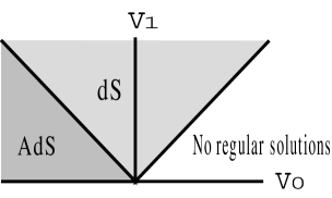
which is similar to that of an axion with an instanton correction. In this paper we consider the two-dimensional parameter space of the scalar field potential,
| (11) |
We may assume to be a positive parameter by shifting , appropriately. In this parameterization the result (10) shows that the parameter region for the existence of a regular de Sitter domain wall solution is given by
| (12) |


III Extension of the de Sitter domain wall space-time
The vanishing points are actually horizons. To show this we will extend the solutions (5). The extended space-time is essentially equivalent to the case of Wang:2002pk , and we will follow their discussions. We first change to a conformal coordinate . Integrating the solution (5), we obtain
| (13) |
where is an integration constant. Using (13) and taking a proper value of , the metric for a de Sitter domain wall solution becomes
| (15) | |||||
where we have changed to a global coordinate of a de Sitter space-time instead of a flat one appearing in (2), and denotes the metric on an -dimensional unit sphere. By a further transformation of and , we obtain
| (16) | |||
| (17) |
Note that the allover factor of the metric (17) is non-singular for all the real values of and . After the change of variables , the metric in the parentheses becomes and is free of a conical singularity. As pointed out in Wang:2002pk , the domain wall peak at is a bubble with a constant acceleration in the coordinate .
As for the scalar field, we obtain
| (18) |
which is also well-defined for any real values of and .
IV Anti-de Sitter domain wall solutions
In the following we will study the other parameter regions of the potential (11) than (12). Looking at the expression (10), one notices that all the other parameter regions of and can be covered by the analytic continuations of the parameters and to pure imaginary values. However, under an analytic continuation of only one of or to a pure imaginary value, one of or becomes imaginary and physically meaningless. This cannot be resolved even by using the constant shift ambiguity of of the solution. To obtain a physically meaningful expression from (5), both of and must be analytically continued to imaginary values, and, after some trials, it turns out that the analytic continuation should contain a simultaneous shift of as 111The other available choices of the shift of do not give any other independent solutions.
| (19) | |||||
| (20) | |||||
| (21) |
where and are real constants and is the elliptic integral of the first kind,
| (22) |
Substituting the analytic continuation (19) into the de Sitter solution (5), we obtain new solutions
| (23) | |||||
| (24) |
and
| (26) | |||||
By the parameterization (11), the scalar potential (26) is in the region
| (27) |

To make the warped metric (2) meaningful under the analytic continuation (19), we perform a simultaneous continuation and . Then (2) becomes an anti-de Sitter domain wall metric
| (28) |
Thus in the region (27), there exist regular AdS domain wall solutions, which are given by (23) and (26).
The stability of the AdS solutions can be checked as follows. We restrict our attention to the five dimensional case (). Presumably the extension to a general dimension will be straightforward. As discussed in DeWolfe ; Gremm:2000dj ; DeWolfe:2000xi ; Kobayashi:2001jd , the problem of obtaining the mass spectra of the linear perturbations around a solution boils down to solving Schrodinger equations. As for the tensor perturbation,
| (29) | |||||
| (30) |
the Schrodinger equation has a supersymmetric form
| (31) |
where
| (32) |
Thus the eigenvalues is non-negative, and hence the stability under the tensor perturbations is satisfied. As for the scalar perturbation,
| (33) |
the Schrodinger equation becomes DeWolfe:2000xi ; Kobayashi:2001jd ; Sasakura
| (34) |
where
| (35) |
This Schrodinger equation is obtained by the substitution in the corresponding expression in Sasakura . The is obviously positive, and the AdS solutions are stable under the scalar perturbations. However there remains one thing to check before this conclusion. If there existed points with , the operator would become singular at these points and the above naive discussion of the positivity would be in danger. Moreover, in the derivation of the Schrodinger equation for the scalar perturbations in Kobayashi:2001jd , the linear perturbation is redefined by a multiplication of a factor which is singular if . But, in the solution (23), is always non-zero, and the above discussion is safe.
V The region without regular solutions
We cannot find a physically meaningful analytic continuation to the parameter region
| (36) |
Thus it is suspected that there are no regular domain wall solutions of the form of the warped metric (2) in this parameter region. To see whether this is the case, we will use a numerical computation.
Since, in this parameter region, the constant part of the scalar potential is larger than that of the parameter region of de Sitter analytic solutions (12), we may assume the solution to be a de Sitter domain wall rather than an anti-de Sitter one. As generally discussed in our previous paper Sasakura , a regular de Sitter domain wall solution is sandwiched between two horizons. The initial values of the differential equations (3) can be provided by the three values , and at a certain initial location of . For the solution to be regular at a horizon, the scale factor must behave in the form (8), and therefore the freedom to choose the initial values is reduced to the only free parameter at the horizon. Thus, to search for a regular solution, we take one of the horizons as the initial location, and integrate numerically the differential equations (3) for each value of at the horizon. Then the question of the existence of a regular solution is translated to whether there exists an initial value for which the numerical solution of the differential equations is regular between the initial horizon and the other horizon of a domain wall.
This search procedure gives a numerical regular solution for each choice of . Studying in this three-dimensional space would be too much, and in fact, we can reduce the dimension to one by rescaling the differential equations (3). By the rescaling of and , we can normalize the scalar potential and the Hubble constant so that and . Thus it is enough to check the question for each choice of .
It would be a reasonable assumption that a domain wall contains the peak of the potential energy . Then, since the potential (11) is invariant222Namely, invariant under ., it is enough for us to solve the equations in the region . We take an initial value and solve the differential equations (3) taking the branch , until the solution reaches the value . By sweeping the initial value , we obtain the range of at . If the obtained range of contains both positive and negative values, one can construct a regular solution by gluing a numerical solution with a certain value of to the image of the solution with . If the range does not contain both signs, one cannot construct a regular solution.
We performed the above procedure in five space-time dimensions . From (12), the maximum value for the existence of an analytic solution is . In fact, for , we obtained for , respectively, and the existence of a regular solution is numerically supported. For , however, the plotted values of in fig.4 indicate that takes only negative values. Thus it is numerically supported that there do not exist any regular de Sitter domain wall solutions in the parameter region (36).

Qualitatively, in this parameter region, the constant part of the scalar field potential is so large that the expansion rate at the core is too large for a domain wall to keep its shape. Similar phenomena are discussed in the context of topological inflation in Vilenkin:1994pv ; Linde:1994hy ; Bonjour:1999kz . In Bonjour:1999kz , a perturbative analysis of the phase boundary between the existence and non-existence of domain wall solutions for the four-dimensional system of gravity and a scalar field was performed, including the present case with an axion-like scalar field potential333Denoted as a sine-Gordon potential in Bonjour:1999kz .. According to the paper, the phase boundary is generally characterized by the equation
| (37) |
in our present notation for . Substituting the parameterization (11), this becomes , which agrees with (36) for .
Thus, in the region (36), the rapid expansion will ultimately sweep away the spatial dependence of the scalar field, and the dynamics will be mainly described by its time-dependence. This will be the subject of section VI.
VI Cosmological solutions
It is well known that, starting from a domain wall solution, a cosmological solution can be obtained by an analytic continuation which exchanges the transverse coordinate and the time coordinate Cvetic:1997vr . An appropriate analytic continuation is given by
| (38) | |||||
| (39) | |||||
| (40) |
by which, a de Sitter domain wall solution (5) changes to a new solution with the substitution and . This analytic continuation turns the de Sitter domain wall metric (2) into
| (41) |
which describes a FRW cosmology of an open universe. Hence the new solution represents a finite lifetime open universe with a big-bang and a big-crunch.
Under the analytic continuation (38), the equations of motion (3) remain the same with the identification of ′ with the time derivative and with and changing the sign of the scalar potential. Under the change of the sign of the potential, the region of the de Sitter solutions (12) is transformed to the identical region. Thus the parameter region for the open universe solution is the same as that of the de Sitter wall solutions (12).
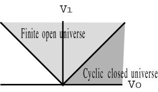
As for the anti-de Sitter solution, the analytic continuation (38) turns it into a cosmological solution of a closed universe. Because of the flip of the sign of the scalar potential, the parameter region of the closed universe solution is obtained by flipping (27) into
| (42) |
This agrees with the region where there are no regular domain wall solutions. The corresponding cosmological solutions are obtained by the substitution and in the AdS domain wall solutions (23). The periodic behavior of the AdS domain wall solutions is now interpreted as representing a cyclic universe.
It would be interesting to see the behavior of the energy density and the pressure. In a five-dimensional space-time, they are
| (43) | |||||
| (44) | |||||
| (45) | |||||
| (46) |
In fig.7, we plotted the time evolution of the energy density and the pressure for the cyclic universe solution with and .


At the minimum of the scale factor the energy density takes its maximum value and the pressure is approximately the minus of the energy density. At this period the large energy density initiates a bounce and the universe is at the inflation stage. On the other hand, at the maximum of the scale factor, the energy density is nearly vanishing and the pressure dominates. The large pressure works as a negative gravitational energy and initiates a contraction of the universe.
For a flat FRW universe, if we assume the null energy condition, the Hubble parameter satisfies an inequality
| (47) |
and there cannot exist a bounce. This also implies that, since our universe is expanding at present days, the universe must have started from a singularity. In the papers Khoury:2001bz ; Seiberg:2002hr , some loopholes of the above discussion are presented from string theory to support the possibility of the pre-big bang scenario Veneziano:2000pz . In our cyclic solution, the existence of the positive curvature of the space changes the equation of motion of into
| (48) |
and can take both signs. Considering the high energy at the big-bang of the universe, it is plausible that some fluctuations of matters and gravity generate a region with a positive spatial curvature and the bounce of the universe simply happens from a classical dynamics. In this case, even though the present model seems far from what is the real universe, it might provide a simple toy model to study the pre-big bang scenario.
The inequality (47) plays also an important role in the dS/CFT correspondence. The central charge is given by an inverse power of the Hubble parameter, and the inequality (47) supports the interpretation of the time evolution as a renormalization group flow to UV Strominger:2001gp ; Balasubramanian:2001nb . In the case of a cyclic universe, however, the time flow cannot be interpreted in this way Argurio , because reverse process exists. If we take seriously the interpretation of Strominger:2001gp ; Balasubramanian:2001nb , there should be a kind of mechanism to prevent the above situation to happen. From this point, it would be interesting to try to consistently embed our simple model into string theory.
VII Summary and discussions
In this paper, we have studied the analytic solutions of the system of gravity and a scalar field with an axion-like potential. They contain de Sitter thick domain walls, anti-de Sitter thick domain walls, finite lifetime universes with a big-bang and a big-crunch, and cyclic universes. These analytic solutions might be useful as toy models for the studies of the more general corresponding cases.
An obvious application of the analytic de Sitter domain wall solutions presented in this and previous papers Sasakura would be as toy models of our world through the brane world scenario. According to the recent observations Fukugita:2000ck , our universe was in the inflation stage at the big-bang, and moreover a tiny cosmological constant might exist even at present. In our model, gravity will be confined by the mechanism of Randall:1999vf , and it would be interesting to investigate the gravitational properties in such an accelerating domain wall universe.
Another interesting direction would be to embed our model into supersymmetric theories or superstring theory. The potential (11) has a simple form of an axion, which would be easily generated by field theory or string theory instanton corrections. According to Witten:2001kn , a de Sitter space-time cannot have any supersymmetries, and hence supersymmetries must be broken on a de Sitter domain wall. In the identification of our world with the domain wall, it seems challenging to explain the large hierarchy between the observed upper bound of the cosmological constant and the supersymmetry breaking scale. Based on a similar motivation, our model may be regarded as a gravity-coupled analogy of the susy-breaking domain wall solution presented in Maru:2001gr ; Maru:2001sk .
Our cosmological solutions of cyclic universes might provide toy models for the scenario of Steinhardt:2001vw ; Felder:2002jk .
Acknowledgements.
The author would like to thank N. Sakai for discussions. The author was supported in part by Grant-in-Aid for Scientific Research (#12740150), and in part by Priority Area: “Supersymmetry and Unified Theory of Elementary Particles” (#707), from Ministry of Education, Science, Sports and Culture, Japan.References
- (1) N. Sasakura, “A de Sitter thick domain wall solution by elliptic functions,” JHEP 0202, 026 (2002) [arXiv:hep-th/0201130].
- (2) M. Cvetic, S. Griffies and S. J. Rey, “Static domain walls in N=1 supergravity,” Nucl. Phys. B 381, 301 (1992) [arXiv:hep-th/9201007].
- (3) C. Csaki, J. Erlich, T. J. Hollowood and Y. Shirman, “Universal aspects of gravity localized on thick branes,” Nucl. Phys. B 581, 309 (2000) [arXiv:hep-th/0001033].
- (4) K. Skenderis and P. K. Townsend, “Gravitational stability and renormalization-group flow,” Phys. Lett. B 468, 46 (1999) [arXiv:hep-th/9909070].
- (5) A. Chamblin and G. W. Gibbons, “Nonlinear supergravity on a brane without compactification,” Phys. Rev. Lett. 84, 1090 (2000) [arXiv:hep-th/9909130].
- (6) O. DeWolfe, D. Z. Freedman, S. S. Gubser and A. Karch, “Modeling the fifth dimension with scalars and gravity,” Phys. Rev. D 62, 046008 (2000) [arXiv:hep-th/9909134].
- (7) M. Gremm, “Thick domain walls and singular spaces,” Phys. Rev. D 62, 044017 (2000) [arXiv:hep-th/0002040].
- (8) E. E. Flanagan, S. H. Tye and I. Wasserman, “Brane world models with bulk scalar fields,” Phys. Lett. B 522, 155 (2001) [arXiv:hep-th/0110070].
- (9) E. Dudas and J. Mourad, “Brane solutions in strings with broken supersymmetry and dilaton tadpoles,” Phys. Lett. B 486, 172 (2000) [arXiv:hep-th/0004165].
- (10) R. Blumenhagen and A. Font, “Dilaton tadpoles, warped geometries and large extra dimensions for non-supersymmetric strings,” Nucl. Phys. B 599, 241 (2001) [arXiv:hep-th/0011269].
- (11) R. Gregory, “Non-singular global strings,” Phys. Rev. D 54, 4955 (1996) [arXiv:gr-qc/9606002].
- (12) P. Berglund, T. Hubsch and D. Minic, “de Sitter spacetimes from warped compactifications of IIB string theory,” Phys. Lett. B 534, 147 (2002) [arXiv:hep-th/0112079].
- (13) C. Charmousis, “Dilaton spacetimes with a Liouville potential,” Class. Quant. Grav. 19, 83 (2002) [arXiv:hep-th/0107126].
- (14) F. Bonjour, C. Charmousis and R. Gregory, “Thick domain wall universes,” Class. Quant. Grav. 16, 2427 (1999) [arXiv:gr-qc/9902081].
- (15) F. Bonjour, C. Charmousis and R. Gregory, “The dynamics of curved gravitating walls,” Phys. Rev. D 62, 083504 (2000) [arXiv:gr-qc/0002063].
- (16) A. h. Wang, “Thick de Sitter brane worlds, dynamic black holes and localization of gravity,” arXiv:hep-th/0201051.
- (17) See for example, M. Cvetic and H. H. Soleng, “Supergravity domain walls,” Phys. Rept. 282, 159 (1997) [arXiv:hep-th/9604090].
- (18) O. DeWolfe and D. Z. Freedman, “Notes on fluctuations and correlation functions in holographic renormalization group flows,” arXiv:hep-th/0002226.
- (19) S. Kobayashi, K. Koyama and J. Soda, “Thick brane worlds and their stability,” Phys. Rev. D 65, 064014 (2002) [arXiv:hep-th/0107025].
- (20) A. Vilenkin, “Topological inflation,” Phys. Rev. Lett. 72, 3137 (1994) [arXiv:hep-th/9402085].
- (21) A. D. Linde, “Monopoles as big as a universe,” Phys. Lett. B 327, 208 (1994) [arXiv:astro-ph/9402031].
- (22) J. Khoury, B. A. Ovrut, N. Seiberg, P. J. Steinhardt and N. Turok, “From big crunch to big bang,” Phys. Rev. D 65, 086007 (2002) [arXiv:hep-th/0108187].
- (23) N. Seiberg, “From big crunch to big bang - is it possible?,” arXiv:hep-th/0201039.
- (24) G. Veneziano, “String cosmology: The pre-big bang scenario,” arXiv:hep-th/0002094.
- (25) A. Strominger, “Inflation and the dS/CFT correspondence,” JHEP 0111, 049 (2001) [arXiv:hep-th/0110087].
- (26) V. Balasubramanian, J. de Boer and D. Minic, “Mass, entropy and holography in asymptotically de Sitter spaces,” Phys. Rev. D 65, 123508 (2002) [arXiv:hep-th/0110108].
- (27) R. Argurio, “Comments on cosmological RG flows,” arXiv:hep-th/0202183.
- (28) See for example, M. Fukugita, “Cosmology and particle physics,” arXiv:hep-ph/0012214.
- (29) L. Randall and R. Sundrum, “An alternative to compactification,” Phys. Rev. Lett. 83, 4690 (1999) [arXiv:hep-th/9906064].
- (30) E. Witten, “Quantum gravity in de Sitter space,” arXiv:hep-th/0106109.
- (31) N. Maru, N. Sakai, Y. Sakamura and R. Sugisaka, “SUSY breaking by stable non-BPS walls,” in C01-07-03.2 arXiv:hep-th/0109087.
- (32) N. Maru, N. Sakai, Y. Sakamura and R. Sugisaka, “SUSY breaking by stable non-BPS configurations,” arXiv:hep-th/0112244.
- (33) P. J. Steinhardt and N. Turok, “A cyclic model of the universe,” arXiv:hep-th/0111030.
- (34) G. N. Felder, A. Frolov, L. Kofman and A. Linde, “Cosmology with negative potentials,” Phys. Rev. D 66, 023507 (2002) [arXiv:hep-th/0202017].