LAPTH-901/2002
DTP-MSU/02-04
Monopoles in NBI-Higgs theory and Born-Infeld collapse

Abstract

Regular magnetic monopoles in the non-Abelian Born-Infeld-Higgs theory are known to exist in the region of the field strength parameter $\beta>\beta_{{\rm cr}}$, bounded from below. Beyond this region, only pointlike (embedded abelian) monopoles exist, and we show that the transition from the regular to singular structure is reminiscent of gravitational collapse. Near the threshold behavior is characterized by the rapidly increasing negative pressure, which typically arises in the high density NBI matter. Another feature, shared both the NBI and gravitating monopoles, is the existence of excited states, which can be thought of as bound states of monopoles and sphalerons. These are labeled by the number $N$ of nodes of the Yang-Mills function. Their masses are greater than the mass of the ground state monopole, and they are expected to be unstable. The sequence of masses $M_{N}$ rapidly converges to the mass of the embedded Abelian solution with constant Higgs. The ratio of the sphaleron size to that of the monopole grows with decreasing $\beta$, and, at the same time, both fall down until the solutions cease to exist, again exhibiting collapse to the pointlike monopole. The results are presented and compared both for the ordinary and the symmetrized trace NBI actions.

1 Introduction

An effective low-energy dynamics of strings attached to multiple D-branes is governed by the non-Abelian Born-Infeld (NBI) action [1, 2]. Different aspects of this theory were studied recently including the problem of magnetic monopoles. The NBI theory contains a parameter, $\beta$, of dimension of the field strength (string tension), reflecting a non-local nature of the underlying string theory. It was observed numerically [3, 4] that monopole solutions exist for $\beta$ varying from infinity (which corresponds to the usual form of the YM action) till some boundary value $\beta_{\rm cr}$, while for $\beta<\beta_{\rm cr}$ only pointlike (embedded abelian) monopoles exist (see also [5, 6]). Previous study [7] also revealed an existence of the excited monopoles in the NBI theory with the similar threshold behavior. Here we study monopoles near the threshold in more details, and find an interesting new phenomenon in the NBI theory, resembling gravitational collapse.

In fact, magnetic monopoles in the Yang-Mills-Higgs (YMH) theory with the standard YM lagrangian coupled to gravity exhibit similar features [8] (for a review and further references see [9, 10]). Gravity imposes an upper limit on the monopole mass, whose physical meaning is simple: when the monopole radius becomes smaller than its gravitational radius, the black hole should be formed. A detailed study of the monopole — black hole transition was undertaken recently by Lue and Weinberg [11, 12]. The ratio of the monopole mass to the Planck mass serves as an order parameter, $\alpha$, describing transition from the globally regular solutions to black holes. Regular solutions exist for $\alpha<\alpha_{\rm cr}$, the critical value $\alpha_{\rm cr}$ being of the order unity. Another feature of the near critical region is the bifurcation of the mass curve, giving rise to new branches of the gravitationally excited monopoles. The latter may be regarded as bound states of monopoles with gravitational sphalerons [13], known as Bartnik-McKinnon’s (BK) solutions [14], which live inside the monopole core. Therefore, the threshold in the parameter space of gravitating monopoles is associated both with the monopole-black hole transition and branching off the gravitationally excited monopoles.

It turns out that the flat space NBI theory admits sphaleron solutions similar to Bartnik-McKinnon particles [15] (though with some differences in the detailed structure [16, 17]). Moreover, when the NBI theory is coupled to gravity, parameters of the NBI sphalerons are continuously driven with the increasing Newton constant to these of the BK particles. Existence of both the BK and the NBI sphalerons is related to breaking of scale invariance of the Yang-Mills theory by non-linearity of the BI lagrangian in the first case, and by gravity in the second. Therefore, the possibility of bound states of the NBI sphalerons with magnetic monopoles could be expected by an analogy with the gravitating case. Note that the limit of vanishing gravity corresponds to the YM limit $\beta\to\infty$ in the case of the NBI theory.

Surprisingly enough, the analogy with gravitation goes farther, and one observes some analog of gravitational collapse in the flat space NBI theory. The size of monopoles (including excited states) is rapidly decreasing when $\beta\to\beta_{\rm cr}$ with the limiting configuration being an Abelian pointlike monopole. An analysis of stresses inside monopoles near the criticality shows that both radial and tangential pressure become negative in the core and rapidly increase. It is expected that in the dynamical picture these stresses will force the regular configuration to shrink to the pointlike structure.

The plan of the paper in as follows. In Sec. 2 we discuss the form of the NBI lagrangian and present the ordinary trace and the symmetrized trace versions of the theory. Sec. 3 contains the description of the monopole-sphaleron bound states in the ordinary trace model. In Sec. 4 we discuss the structure of solutions near the threshold and reveal the collapse behavior for both the ground and excited monopoles. In sec. 5 the analogous results are briefly discussed within the symmetrized trace NBI model.

2 The action

A subtle point in the definition of the NBI action is the specification of the trace over the gauge group generators [1, 18, 19, 20, 21, 22] (for an earlier discussion see [23]). Formally a number of possibilities can be envisaged. Starting with the determinant form of the $U(1)$ Dirac-Born-Infeld action

$$S=\frac{1}{4\pi}\int\left\{1-\sqrt{-\det(g_{\mu\nu}+F_{\mu\nu})}\right\}d^{4}x,$$ (1)

one has different options including the usual trace, the symmetrized or antisymmetrized traces [1], or evaluation of the determinant both with respect to Lorenz and the gauge matrix indices [21]. Alternatively, one can start with the Abelian ‘square root’ form, which is obtained in the four-dimensional case evaluating the determinant under the square root:

$$\sqrt{-\det(g_{\mu\nu}+F_{\mu\nu})}=\sqrt{-\det(g)}\;\sqrt{1+\frac{1}{2}F^{2}-\frac{1}{16}(F\tilde{F})^{2}},$$ (2)

with $F^{2}=F_{\mu\nu}F^{\mu\nu},\;F\tilde{F}=F_{\mu\nu}\tilde{F}^{\mu\nu}$. For a non-Abelian gauge group this relation is no more valid, unless a special trace prescription is made, but this U(1) action may serve as another starting point for non-Abelian generalization applying the simple trace to the right hand side of this equation.

A particular trace operation, for which the relation Eq.(2) remains valid, is the ‘symmetrized trace’ suggested by Tseytlin [1]. The original argument was that in the non-Abelian case the commutators of the field strength tensors can be expressed via their derivatives, these should be absent within the constant field approximation in which the NBI action s derived in the string theory. The trace definition eliminating commutators involves the symmetrization of all products of the generators obtained in the power series expansion of the square root. Independently of whether this prescription corresponds indeed to the string theory result in all orders in $\beta$ (actual calculations shows that it may be not true in higher orders [24, 25, 26]), this is a valuable model to be considered.

The explicit form of the SU(2) NBI action with the symmetrized trace for static $SO(3)$-symmetric magnetic type configurations was found in [16]. One starts with the definition

$$L^{str}_{NBI}=\frac{\beta^{2}}{4\pi}\mathop{\rm Str}\nolimits\left(1-\sqrt{-\det\Bigl{(}g_{\mu\nu}+\frac{1}{\beta}F_{\mu\nu}\Bigr{)}}\right)=k\frac{\beta^{2}}{4\pi}\mathop{\rm Str}\nolimits(1-\mathcal{R}),$$ (3)

where

$$\mathcal{R}=\sqrt{1+\frac{1}{2\beta^{2}}F_{\mu\nu}F^{\mu\nu}-\frac{1}{16\beta^{4}}(F_{\mu\nu}{\tilde{F}}_{\mu\nu})^{2}},$$ (4)

and $\beta$ of the dimension of length^-2 is the BI ’critical field’. Assuming the usual spherically symmetric t’Hooft-Polyakov ansatz

$$A^{a}_{0}=0\qquad A^{a}_{i}=\epsilon_{aij}\frac{n^{j}}{r}(1-w(r)),$$ (5)

where $n^{k}=x^{k}/r$, $r=\sqrt{x^{2}+y^{2}+z^{2}}$ and $w(r)$ is the real valued function, the lagrangian (3) is evaluated by expanding the square root in powers of $F$, performing symmetrization of all products of the gauge generators, evaluating the trace, and finally summing up the resulting expansion. The result is the following [16]:

$$L^{str}_{NBI}=\frac{\beta^{2}}{4\pi}\left(1-\frac{1+V^{2}+K^{2}\mathcal{A}}{\sqrt{1+V^{2}}}\right),$$ (6)

where

$$V^{2} = \frac{(1-w^{2}(r))^{2}}{\beta^{2}r^{4}},\quad K^{2}=\frac{w^{\prime 2}(r)}{\beta^{2}r^{2}},$$

$$\mathcal{A} = \sqrt{\frac{1+V^{2}}{V^{2}-K^{2}}}\mathop{\mathrm{arctanh}}\sqrt{\frac{V^{2}-K^{2}}{1+V^{2}}},$$ (7)

and dash denotes derivative with respect to $r$. This form of the lagrangian is appropriate for $V^{2}>K^{2}$, otherwise the function $\mathop{\mathrm{arctanh}}$ could be replaced by $\arctan$. Note that, when the difference $V^{2}-K^{2}$ changes sign, the function $\mathcal{A}$ remains real valued.

The action with an ordinary trace applied to the square root form (2) reads

$$L^{tr}_{NBI}=\frac{\beta^{2}}{4\pi}\left(1-\sqrt{1+V^{2}+2K^{2}}\right).$$ (8)

It can be checked that, as $\beta\to\infty$, the standard Yang-Mills lagrangian (restricted to the monopole ansatz) is recovered in both cases. But in the strong field region the two expressions differ substantially.

The total action to be used here is the sum $S=S_{NBI}+S_{H}$, where the Higgs part is taken in the usual form

$$S_{H}=\frac{1}{8\pi}\int\left(D_{\mu}\phi^{a}D^{\mu}\phi^{a}-\frac{\lambda}{2}\left(\phi^{a}\phi^{a}-v^{2}\right)\right).$$ (9)

Here the dimensionless gauge coupling constant (in units $\hbar=c=1$) is set to unity, so we have three parameters: the Higgs expectation value $v$, Higgs self-interaction constant $\lambda$ and the BI critical field $\beta$. By additional rescaling, the constant $v$ can be set to unity. For the Higgs field the standard hedgehog ansatz is assumed:

$$\phi^{a}=\frac{H(r)}{r}n^{a}.$$ (10)

3 NBI sphalerons inside monopoles

We start with the square root form of the NBI action (8). Performing an integration over spherical angles one obtains the one-dimensional reduced action, equal to minus the energy functional:

$$S=-4\pi\int dr\,r^{2}\left\{\beta^{2}({\cal R}-1)+\frac{1}{2r^{2}}\left((H^{\prime}-\frac{H}{r})^{2}+\frac{2}{r^{2}}H^{2}w^{2}\right)+\frac{\lambda}{4}\left(\frac{H^{2}}{r^{2}}-1\right)^{2}\right\},$$ (11)

where

$${\cal R}=\sqrt{1+\frac{2}{\beta^{2}r^{4}}(r^{2}w^{\prime 2}+\frac{1}{\beta^{4}}(w^{2}-1)^{2})}.$$ (12)

Variation of this functional leads to the following equations of motion

$$r^{2}w^{\prime\prime} = w({\cal R}H^{2}+w^{2}-1)+r^{2}\frac{{\cal R}^{\prime}}{{\cal R}}w^{\prime},$$ (13)

$$r^{2}H^{\prime\prime} = 2Hw^{2}-\lambda H(r^{2}-H^{2})\;.$$ (14)

Boundary conditions at infinity for the monopole solutions read

$$\lim_{r\to\infty}w(r)=0,\qquad\lim_{r\to\infty}\frac{H(r)}{r}=1,$$ (15)

while regularity at the origin implies

$$w(0)=1,\qquad H(0)=0.$$ (16)

Starting with the values (16), one can construct the following power series solution converging in some domain around the origin:

$$w = 1-br^{2}+\frac{\beta b^{2}\left(22b^{2}+\beta^{2}\right)+d^{2}\left(6b^{2}+\beta^{2}\right)^{\frac{3}{2}}}{10\beta\left(2b^{2}+\beta^{2}\right)}\,r^{4}+O(r^{6}),$$ (17)

$$H = d\,r^{2}-\left(\frac{1}{10}\lambda d+\frac{2}{5}d\,b\right)r^{4}+O(r^{6}),$$ (18)

where $b$ and $d$ are free parameters. Solutions which start at the origin in this way reach monopole asymptotics (15) for some discrete values of $b$ and $d$. The equations reduces to those of the standard YMH-theory as $\beta\to\infty$. In [3] it was shown that monopole solutions to the Eq.(13-14), generalizing the usual t’Hooft–Polyakov monopole, continue to exist for all finite $\beta$ greater than some limiting value $\beta_{cr}$ of the order unity. Here we investigate in more details what happens in the critical region.

The situation resembles that of gravitating monopoles, i.e. solutions of the Einstein-Yang-Mills-Higgs equations [8]. In that case there is a critical value of the gravitational constant (with other parameters fixed) after which regular monopoles cease to exist. In the critical region the gravitational interaction becomes strong and the new solution with the monopole asymptotics arise, which look like bound states of the monopole with the Bartnik-McKinnon particles [8], the latter being solutions of the Einstein-Yang-Mills equations without Higgs. The bifurcation of the monopole branch giving rise to excited monopoles occurs in the vicinity of the critical value of the gravitational constant, the detailed picture depending on the Higgs mass.

The analogy with gravitating monopoles is based on the fact that in the flat space NBI theory (without Higgs) there also exist sphaleron type particle-like solutions [15]. In this case the Derrick’s obstruction is overpassed due to violation of the scale invariance by the NBI action. Therefore, one might expect the existence of bound states of monopoles with NBI sphalerons inside. The structure of these solutions can be described as follows. Near the origin the Higgs field is almost zero, so the influence of the term $H^{2}K{\cal R}$ in the equations of motion is small, and the NBIH system behaves similarly to the NBI one. As was argued in [15], NBI theories with different $\beta$ are equivalent up to rescaling, so, for $\beta$ large enough, the formation of NBI sphalerons starts close to the origin. Outside their core the Higgs field becomes significant, and the solution in the far zone is driven to the monopole configuration. More precisely, in the region of $r\approx 1/\sqrt{\beta}$, the function $w(r)$ is similar to that is the sphaleron type solutions of [15]: starting with $w=1$ it passes through zero and (possibly) oscillates $N$ times before the solution is driven to an asymptotic regime. This time, however, the function $w$ tends not to one of its vacuum values $w=\pm 1$, but is captured to the monopole asymptotic $w=0$. The Higgs field $H(r)$ behaves qualitatively in the same way as in the ground state monopole solutions. These considerations can be converted into the rigorous proof of existence, like in the case of NBI sphalerons [15].

Therefore, for large enough $\beta$, one expects to find the solutions which can be thought of as bound states of the t’Hooft-Polyakov monopole (slightly distorted by the Born-Infeld nonlinearity) and a very small (of size $\approx\beta^{\frac{1}{2}}$) sphaleron sitting in the monopole core. Numerically one finds the whole family of excited monopoles which corresponds to the family of solutions discovered in [15]. They are labeled by the number $N$ of nodes of the function $w$, the $N=0$ solution being the ground sate NBI monopole.

The second parameter which enters the lagrangian (11) is the self-coupling parameter $\lambda$ of the Higgs field. One can see from the equation of motions that the respective terms are small in the deep core, where the excited solutions are starting to form. In the region of near critical $\beta$, all happens in the close vicinity of the origin, so solutions are little sensitive to the values of $\lambda$. Numerical calculations show that the parameters $b$ and $d$ of the excited solutions remain practically unchanged when $\lambda$ is doubled. This is not true for the ground state $N=0$ monopole, which mostly inherits properties of the Yang-Mills-Higgs solution, but one observes that the role of the $\lambda$-depending terms also decreases while approaching the critical region. In particular, the value of $\beta_{cr}$ is independent of $\lambda$.

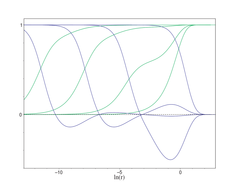
Figure 1: Ground state monopole and three first excited states for $\beta=300$. Blue line — gauge function $w$, green line — Higgs field $H/r$.

Numerical solutions were constructed starting with the regular initial conditions in the origin (16) in terms of the logarithmic variable $t=\ln(r)$ and applying the shooting strategy to find the discrete values of parameters $b$ and $d$ which ensure that the monopole asymptotic conditions (17-18) are fulfilled after several oscillations of $w$. The initial guess for the values of $b$ is provided by the glueball values found in [15]. Dependence of $b$ on $N$ and $\beta$ is shown on the Tab. 2. The other parameter, $d$, turns out to be weakly sensitive to the value of $\beta$ and tends to a constant, as $\beta$ approaches infinity (Tab. 3). The sample solutions for $N=1,2,3$ are shown on Fig. 1 together with the ground state monopole for $\lambda=1$ and $\beta=30$.

4 Born-Infeld collapse

This simple picture holds if the size of sphalerons inside the monopoles is small as compared with the size of the unexcited monopole. However, with decreasing $\beta$, the ratio of the sphaleron radius to that of the monopole increases. At the same time, both radii rapidly fall down. Numerically it is observed that for large enough $\beta$ the parameter $b$ first goes down with decreasing $\beta$), causing the expansion of the NBI glueball (the region of $w$-oscillations). On the other hand, the monopole radius stabilizes for sufficiently small $\beta$ (see [3]), so both sizes become comparable for certain $\beta$. With $\beta$ further decreasing, the YM parameter $b$ in (17-18) starts to increase, as well as the Higgs parameter $d$. The whole solution then acquires the following structure: the function $w$, starting from the value $w=1$, rapidly falls down, performs several oscillations of small amplitude around zero, and approaches zero asymptotically. The Higgs variable $H/r$ does not have any peculiarities: starting from initial value it monotonically grows up to the vacuum expectation value. For smaller $\beta$, the both parameters $b$ and $d$ begin to grow faster and faster and for the critical value $\beta_{cr}$ they tends to infinity. In terms of the logarithmic radial variable $t=\ln r$ one clearly sees that shapes of $w$ and $H/r$ remain almost the same while $\beta$ approaches the critical value, but the whole picture moves to negative $t$ (Tab. 1). This means that the region of the localization of essentially nonabelian structure becomes smaller and smaller, while in the outer region the solution looks like an embedded Abelian monopole

$$w=0,\qquad\frac{H}{r}=1.$$ (19)

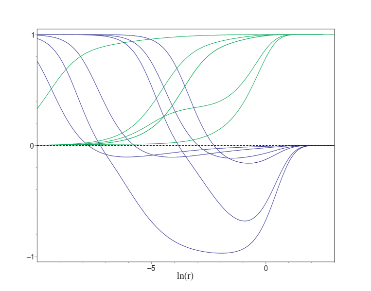
Figure 2: The $N=1$ monopole-sphaleron bound state for $\beta=1,1.05,1.5,10,10^{3},10^{6}$. The Blue line — $w$, the green line — $H/r$. Solutions can be distinguished by their values in the region $\ln r\approx-0.5$: values of $w$ grow up with increasing $\beta$, while values of the Higgs field go down.

The figure 2 illustrates this behavior for the lowest excited solution $N=1$. The functions $w$ and $H$ are plotted for various $\beta$, from very large, up to ones slightly exceeding $\beta_{cr}$. It is seen that the YM function starts to fall down for smaller and smaller values of the radial coordinate when criticality is approached. Similar picture hold for excited solutions with any number of nodes. This collapse process is observed also for the ground state monopole $N=0$ near the critical value $\beta_{cr_{0}}$, approaching which the solution shrinks to the abelian counterpart. The numerical experiments indicate that the critical values of $\beta$ are independent of $\lambda$. For $N\geq 2$, the value $\beta_{cr_{0}}$ is practically independent on $N$ and is equal to $\beta_{{cr}_{2}}\approx 1.03$. For $N=1$ the collapse occurs at $\beta_{{cr}_{1}}\approx 0.92$ while for the ground state monopole $\beta_{{cr}_{0}}\approx 0.52$.

Physical reason for the Born-Infeld collapse can be understood as follows. At high density, the stress-energy tensor of the NBI field develops large negative pressure. From the lagrangian (8) one can derive the following relation for the sum of principal pressures $p_{r}=T_{rr},\,p_{\phi}=T_{\phi\phi}$:

$$2p_{\phi}+p_{r}=f(\rho)=-\frac{\rho(\rho-2\beta^{2})}{\rho+2\beta^{2}},$$ (20)

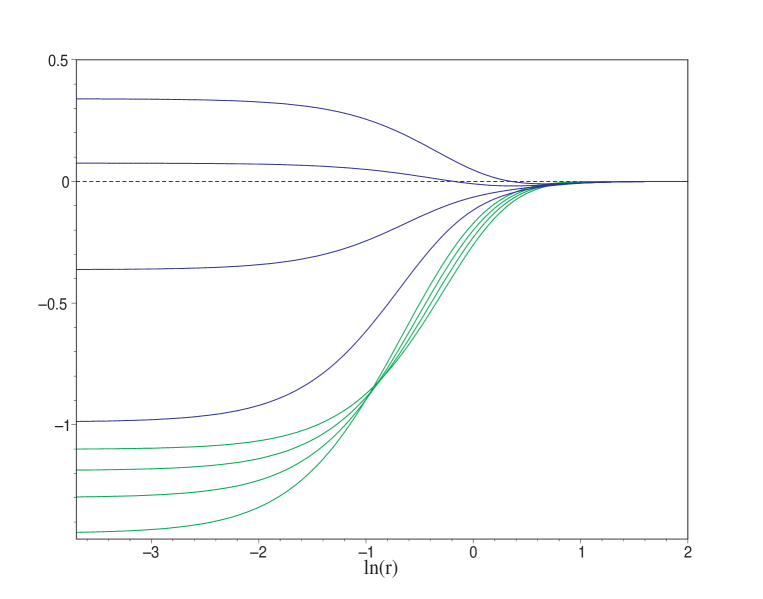
Figure 4: The radial pressure $p_{r}$ for the ground state BI-monopole for $\beta=0.9,1.0,1.2,2.0$. The blue line — the pressure of the NBI field, the green line — the pressure of the Higgs field. The left asymptotic values go down with decreasing $\beta$ for both fields.

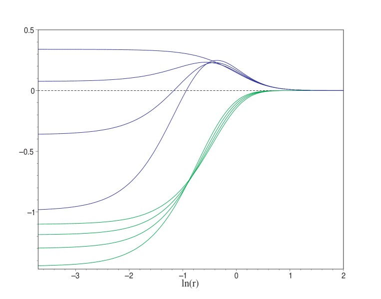
Figure 5: The tangential pressures $p_{\phi}$ behave similarly to those on previous picture

where $\rho=T_{tt}$ is the energy density. This quantity becomes negative for $\rho>2\beta^{2}$. Numerical data for the radial and tangential pressures corresponding to the ground state monopole are given in Figs. 4,5 for the pure gauge component and together with Higgs. When $\beta$ goes to the critical value, the tangential pressure exhibits a small positive knob near the monopole boundary and then becomes negative in the core region. With decreasing $\beta$ it falls down rapidly tending to minus infinity at the threshold. The radial pressure near the threshold is always negative and also tend to minus infinity.

The masses of solutions in the critical region rapidly converge to the energy of the embedded Abelian pointlike monopole (recall that in the Born-Infeld theory the singular pointlike solution 19 has a finite energy):

$$E_{lim}=\int dr\,r^{2}2\beta^{2}({\cal R}-1)=\sqrt{\beta}\int dx\,x^{2}(\sqrt{1+\frac{2}{x^{4}}}-1)=1.23604978\sqrt{\beta}.$$ (21)

This value serves as the upper bound for the mass as a function of $\beta$ and $N$. Moreover, this value describes pretty well the masses of all excited solutions starting from $N=1$: for all $\beta$ the discrepancy does not exceed 3% and it decreases fast near the threshold. This can be seen on Figure 3, showing the masses of $N=0,1,2$ solutions as a function of $\beta$. The bifurcation pattern of the main branch with excited branches is similar to that of gravitating monopoles, but now it occurs with a decreasing parameter.

5 Symmetrized trace model

Within the symmetrized trace model the equations of motion read:

$$\frac{d}{dr}\left\{\frac{w^{\prime}}{2(V^{2}-K^{2})}\left(\frac{K^{2}\sqrt{1+V^{2}}}{1+K^{2}}-\frac{(2V^{2}-K^{2}){\cal A}}{\sqrt{V^{2}-K^{2}}}\right)\right\}=$$

$$\frac{Vw(K^{2}{\cal A}-V^{2})}{(V^{2}-K^{2})\sqrt{1+V^{2}}}+\frac{w\,H^{2}}{r^{2}}$$ (22)

$$r^{2}\,H^{\prime\prime}=H(H^{2}-r^{2})\lambda+2Hw^{2},$$ (23)

where $V$ and $K$ are defined in (2).

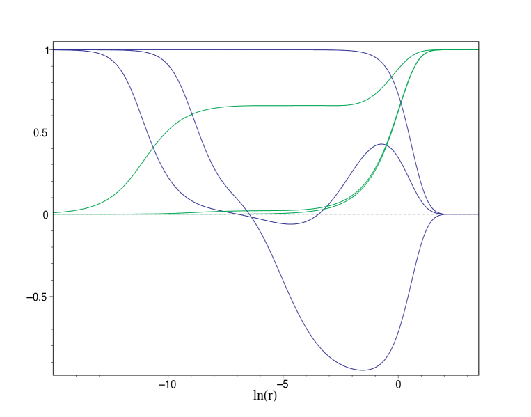
Figure 6: The monopole-sphaleron bound states in the symmetrized trace model for $\beta=10^{6}$. Blue line — gauge function $w$, green line — Higgs field $H/r$.

The pure NBI model with the symmetrized trace also possesses the sphaleronic type excitations which are qualitatively the same as in the ordinary trace model [16]. In particular, the same scaling behavior follows immediately from the action (6). Hence the above arguments about the existence of monopole-sphaleron bound states apply directly, and one can expect to find sphaleronic excitations at least for large $\beta$. Numerical experiments indicate that for large values of $\beta$ there are indeed excited monopole solutions analogous to those considered above (Fig. 6). But, since the structure of the essentially nonabelian region is not the same in both models, there are some differences in the behavior of the solution with varying $\beta$. One observes that, in the symmetrized trace model, the sphaleronic solutions for a given node number $N$ are smaller than those in the ordinary trace model. Also, the amplitude of $w$-oscillations is relatively smaller. All this is reflected in the relatively large values of the parameters $b$ and $d$ which now grow much faster with increasing $\beta$ and $N$.

As a consequence, the collapse, which takes place in this model also, occurs at larger values of $\beta$ for any positive $N$. Moreover, for any given $\beta$, there exist excited solutions only up to some finite $N$, the boundary value of $N$ being dependent on $\beta$.

6 Discussion

Our purpose was to describe an astonishing similarity between gravitating monopoles and those in the flat space non-Abelian Born-Infeld theory. Both theories contain ground state monopoles as well as excited monopoles which can be regarded as bound states of monopoles and sphalerons. In both cases there is a threshold in the parameter space, which marks the end of the monopole sequence. In the gravitating case this happens since the monopole radius becomes smaller that its gravitational radius, so it is the gravitational collapse phenomenon which stands behind this picture. Physically, gravitational collapse can be attributed to development of strong attractive forces when the event horizon is approached. Surprisingly enough, we observed an analogous behavior in in the flat space NBI theory. The size of monopoles (including their excited states) become smaller and smaller when a certain threshold value of the BI field strength parameter is approached, and no extended monopoles exist beyond the threshold. In this region the large negative pressure (tension) is developed inside the regular NBI monopoles, which cause them to shrink to a singular pointlike (Abelian) monopole. Large negative pressure developed inside the high density ball of the NBI matter apparently should create an instability against the contraction to the pointlike structure. The dynamical picture of the collapse phenomenon in the NBI theory is currently under investigation.

It is worth noting, that if one couples the NBI model to gravity, a continuous interpolation between the NBI sphalerons and Bartnik-McKinnon particles is observed [17]. It is expected that parameters of monopole-sphaleron bound states will also exhibit the analogous transition.

$\beta$	$N=0$	$r_{w},N=1$	$r_{h},N=1$	$r_{w},N=2$	$r_{h},N=2$
$10^{6}$	1.399	$.7175\cdot 10^{-3}$	.5082	$.9212\cdot 10^{-4}$	.4970
$10^{4}$	1.399	$.7152\cdot 10^{-2}$	.4512	$.8348\cdot 10^{-3}$	.2970
100	1.399	.05451	.01876	$.1529\cdot 10^{-2}$	$.4325\cdot 10^{-3}$
10	1.397	.1036	.02614	$.2335\cdot 10^{-2}$	$.6372\cdot 10^{-3}$
5	1.391	.1126	.02692	$.2081\cdot 10^{-2}$	$.5500\cdot 10^{-3}$
2	1.349	.08349	.01790	$.6481\cdot 10^{-3}$	$.1542\cdot 10^{-3}$
1.5	1.303	.05188	.01058	$.1690\cdot 10^{-3}$	$.3766\cdot 10^{-4}$
1.2	1.235	.01930	$.3783\cdot 10^{-2}$	$.1102\cdot 10^{-4}$	$.2285\cdot 10^{-5}$
1.15	1.215	.013325	$.2595\cdot 10^{-2}$	$.3863\cdot 10^{-5}$	$.7881\cdot 10^{-6}$
1.1	1.191	$.7755\cdot 10^{-2}$	$.1502\cdot 10^{-2}$	$.8085\cdot 10^{-6}$	$.1620\cdot 10^{-6}$
1.	1.124	$.4249\cdot 10^{-3}$	$.8130\cdot 10^{-4}$	—	—
.97	1.096	$.7122\cdot 10^{-5}$	$.1350\cdot 10^{-5}$	—	—
.8	.7936	—	—	—	—
.7	.4267	—	—	—	—
.6	.1060	—	—	—	—
.55	.02596	—	—	—	—
.526	$.2739\cdot 10^{-2}$	—	—	—	—

Table 1: This table illustrates the behavior of effective sizes of the monopole and the monopole-sphaleron bound states $N=1,2$ with decreasing $\beta$. The sizes are defined as follows: for N=0 it is the distance where the gauge function falls down by half, i.e. $w(r)=0.5$; for N=1,2 the ’sphaleron radius’ $r_{w}$ is the first node of $w$, while the ’monopole radius’ $r_{h}$ is the distance where $H(r)/r=.5$

$\beta$	$N=0$	$N=1$	$N=2$
$10^{6}$	.4496	$.18011\cdot 10^{8}$	$.1258\cdot 10^{10}$
$10^{4}$	.4496	$.1816\cdot 10^{6}$	$.1533\cdot 10^{8}$
100	.4496	3448.	$.4611\cdot 10^{7}$
10	.4519	1089.	$.2141\cdot 10^{7}$
5	.4592	1027.	$.2946\cdot 10^{7}$
2	.5198	2598.	$.4073\cdot 10^{8}$
1.5	.5978	8100.	$.7163\cdot 10^{9}$
1.2	.7496	$.6868\cdot 10^{5}$	$.2046\cdot 10^{12}$
1.15	.8007	$.1524\cdot 10^{6}$	$.1739\cdot 10^{13}$
1.1	.8677	$.4673\cdot 10^{6}$	$.4169\cdot 10^{14}$
1	1.086	$.1699\cdot 10^{9}$	—
.97	1.189	$.6261\cdot 10^{12}$	—
.8	2.951	—	—
.7	9.954	—	—
.60	142.1	—	—
.55	2314.	—	—
.526	$.2070\cdot 10^{6}$	—	—

Table 2: The numerical values of the parameter $b$ of the expansion of $w$ near the origin for various $\beta$

$\beta$	$N=0$	$N=1$	$N=2$
$10^{6}$	1.068	35.69	792.3
$10^{4}$	1.068	36.20	896.1
100	1.068	36.70	1483.
10	1.069	23.88	1007.
5	1.072	23.15	1171.
2	1.096	35.41	4229.
1.5	1.124	60.74	$.1744\cdot 10^{5}$
1.2	1.173	171.8	$.2898\cdot 10^{6}$
1.15	1.188	253.0	$.8420\cdot 10^{6}$
1.1	1.207	439.3	$.4105\cdot 10^{7}$
1.	1.264	8215.	—
.97	1.289	$.4962\cdot 10^{6}$	—
.8	1.638	—	—
.7	2.498	—	—
.6	7.838	—	—
.55	29.63	—	—
.526	273.3	—	—

Table 3: The numerical values of the parameter $d$ of the Higgs field expansion near the origin for various $\beta$

Figure 3: The masses of the ground state monopole $(N=0)$ and $N=1,2$ excited monopoles. The dotted line is the mass of embedded abelian solution (21). The $N=2$ mass curve, in the region where this solution exists, is indistinguishable from mass of the embedded abelian monopole.

References

- [1] A. A. Tseytlin. On non-abelian generalisation of the Born-Infeld action in string theory. Nucl. Phys., B501:41–52, 1997, hep-th/9701125.
- [2] Amit Giveon and David Kutasov. Brane dynamics and gauge theory. Rev. Mod. Phys., 71:983–1084, 1999, hep-th/9802067.
- [3] N. Grandi, E. F. Moreno, and F. A. Schaposnik. Monopoles in non-abelian Dirac-Born-Infeld theory. Phys. Rev., D59:125014, 1999, hep-th/9901073.
- [4] N. Grandi, R. L. Pakman, F. A. Schaposnik, and Guillermo A. Silva. Monopoles, dyons and theta term in Dirac-Born-Infeld theory. Phys. Rev., D60:125002, 1999, hep-th/9906244.
- [5] Prasanta K. Tripathy and Fidel A. Schaposnik. Monopoles in non-Abelian Einstein-Born-Infeld theory. Phys. Lett., B472:89–93, 2000, hep-th/9911065.
- [6] Prasanta K. Tripathy. Gravitating monopoles and black holes in Einstein-Born- Infeld-Higgs model. Phys. Lett., B458:252–256, 1999, hep-th/9904186.
- [7] Dmitri Galtsov and Vladimir Dyadichev. D-branes and vacuum periodicity. Proc. NATO ARW Non-commutative structures in mathematics and physics, Kiev, Ukraine, Sept. 24-28, 2000; S. Duplij and J. Wess (Eds), Kluwer, pages 61–78, 2000, hep-th/0012059.
- [8] Peter Breitenlohner, Peter Forgacs, and Dieter Maison. Gravitating monopole solutions. 2. Nucl. Phys., B442:126–156, 1995, gr-qc/9412039.
- [9] Mikhail S. Volkov and Dmitri V. Gal’tsov. Gravitating non-abelian solitons and black holes with Yang- Mills fields. Phys. Rept., 319:1–83, 1999, hep-th/9810070.
- [10] D. V. Gal’tsov. Gravitating lumps. 2001, hep-th/0112038.
- [11] Arthur Lue and Erick J. Weinberg. Magnetic monopoles near the black hole threshold. Phys. Rev., D60:084025, 1999, hep-th/9905223.
- [12] Arthur Lue and Erick J. Weinberg. Gravitational properties of monopole spacetimes near the black hole threshold. Phys. Rev., D61:124003, 2000, hep-th/0001140.
- [13] D. V. Galtsov and M. S. Volkov. Sphalerons in Einstein Yang-Mills theory. Phys. Lett., B273:255–259, 1991.
- [14] R. Bartnik and J. Mckinnon. Particle - like solutions of the Einstein Yang-Mills equations. Phys. Rev. Lett., 61:141–144, 1988.
- [15] Dmitri Gal’tsov and Richard Kerner. Classical glueballs in non-Abelian Born-Infeld theory. Phys. Rev. Lett., 84:5955–5958, 2000, hep-th/9910171.
- [16] V. V. Dyadichev and D. V. Gal’tsov. Sphaleron glueballs in NBI theory with symmetrized trace. Nucl. Phys., B590:504–518, 2000, hep-th/0006242.
- [17] V. V. Dyadichev and D. V. Gal’tsov. Solitons and black holes in non-Abelian Einstein-Born- Infeld theory. Phys. Lett., B486:431–442, 2000, hep-th/0005099.
- [18] Jerome P. Gauntlett, Joaquim Gomis, and Paul K. Townsend. BPS bounds for worldvolume branes. JHEP, 01:003, 1998, hep-th/9711205.
- [19] D. Brecher. BPS states of the non-abelian Born-Infeld action. Phys. Lett., B442:117–124, 1998, hep-th/9804180.
- [20] D. Brecher and M. J. Perry. Bound states of D-branes and the non-Abelian Born-Infeld action. Nucl. Phys., B527:121–141, 1998, hep-th/9801127.
- [21] Jeong-Hyuck Park. A study of a non-Abelian generalization of the Born-Infeld action. Phys. Lett., B458:471–476, 1999, hep-th/9902081.
- [22] Marija Zamaklar. Geometry of the nonabelian DBI dyonic instanton. Phys. Lett., B493:411–420, 2000, hep-th/0006090.
- [23] T. Hagiwara. A nonabelian Born-Infeld lagrangian. J. Phys., A14:3059, 1981.
- [24] Andrea Refolli, Alberto Santambrogio, Niccolo Terzi, and Daniela Zanon. contributions to the nonabelian Born–Infeld action from a supersymmetric Yang–Mills five-point function. Nucl. Phys., B613:64–86, 2001, hep-th/0105277.
- [25] E. A. Bergshoeff, A. Bilal, M. de Roo, and A. Sevrin. Supersymmetric non-abelian Born–Infeld revisited. JHEP, 07:029, 2001, hep-th/0105274.
- [26] Alexander Sevrin, Jan Troost, and Walter Troost. The non-abelian Born–Infeld action at order . Nucl. Phys., B603:389–412, 2001, hep-th/0101192.