The Spectrum of the Neumann Matrix with Zero Modes

Abstract:

We calculate the spectrum of the matrix $M^{\prime}$ of Neumann coefficients of the Witten vertex, expressed in the oscillator basis including the zero-mode $a_{0}$. We find that in addition to the known continuous spectrum inside $[-\frac{1}{3},0)$ of the matrix $M$ without the zero-modes, there is also an additional eigenvalue inside $(0,1)$. For every eigenvalue, there is a pair of eigenvectors, a twist-even and a twist-odd. We give analytically these eigenvectors as well as the generating function for their components. Also, we have found an interesting critical parameter $b_{0}=8\ln 2$ on which the forms of the eigenvectors depend.

1 Introduction

Vacuum String Field Theory (VSFT) was proposed by Rastelli, Sen and Zwiebach in [1] - [7] as the expansion of Witten’s Open String Field Theory [8] around the non-perturbative vacuum. They conjectured that the kinetic operator of VSFT is pure ghost after a suitable (possibly singular) field redefinition. A strong support of this conjecture was that they could reproduce numerically, with convincing precision, the correct D-brane descent relations [2]. These descent relations were further established in the context of Boundary Conformal Field Theory [4]. However, until recently, a direct algebraic derivation based on the properties of the Neumann coefficients has been elusive; and so have been the proofs of other conjectures, such as the equality between the algebraic and the geometric sliver, or the form of the pure-ghost kinetic operator around the stable vacuum.

These proofs all came up very recently, shortly after Rastelli, Sen and Zwiebach solved the spectrum of the matrix $M$ of Neumann coefficients [9]. They found that the spectrum is continuous in the range $[-{1\over 3},0)$; every eigenvalue in this interval is doubly degenerate, except for $-{1\over 3}$ which is single and twist-odd. They gave a complete solution by finding the density of eigenvalues and the expressions of the corresponding eigenvectors. This result turned out to be a key tool for doing exact calculations in VSFT. Indeed, using the form of the spectrum of $M$, Okuyama [10] proved that the ghost kinetic operator of VSFT is given by the ghost field $c$ evaluated at the string midpoint, as was already expected [11, 6]. Then in another paper [12], Okuyama also gave an algebraic proof that the D-brane descent relation is correctly reproduced. The ration of the tension of a D$p$-brane to the tension of a D$(p+1)$-brane can be expressed in terms of determinants of matrices of Neumann coefficients

$$R={T_{p}\over 2\pi\sqrt{\alpha^{\prime}}T_{p+1}}={3\left(V_{00}^{rr}+{b\over 2}\right)^{2}\over\sqrt{2\pi b^{3}}}{\det(1-M^{\prime})^{3\over 4}(1+3M^{\prime})^{1\over 4}\over\det(1-M)^{3\over 4}(1+3M)^{1\over 4}}\,,$$ (1)

where $M$ is the matrix formed by the Neumann coefficients of the vertex in the oscillator basis with zero momentum, whereas $M^{\prime}$ is made out of the Neumann coefficients of the vertex expressed in the oscillator basis including the zero-mode oscillator $a_{0}$. The parametre $b$ is an arbitrary constant in the definition $a_{0}^{\mu}:=\frac{1}{2}\sqrt{b}p^{\mu}-\frac{1}{\sqrt{b}}ix^{\mu}$ [2]. Although it seems, at a first look, that one needs the spectrum of both $M$ and $M^{\prime}$ to calculate $R$, Okuyama [12] found an elegant way of calculating this ratio knowing only the spectrum of $M$. At last, Okuda [13] proved the equality of the geometric sliver and the algebraic sliver [2, 5, 14, 15, 16, 17].

Because the spectrum of $M$ is such an important piece of data, it is reasonable to expect that knowing the spectrum of $M^{\prime}$ will be very useful as well. In this paper we thus solve the problem of finding all eigenvalues and eigenvectors of $M^{\prime}$.

We summarize our results here: We find that the eigenvalues of $M^{\prime}$ are given by two types, a continuous and a discrete spectrum. The continuous eigenvalues are the same as that of $M$ and are located in the range $[-1/3,0)$. The discrete eigenvalue is located in the range $(0,1)$ and is determined by (59) (or (60)) implicitly. The corresponding eigenvectors are as follows. For every eigenvalue $\lambda\in[-1/3,0)$, we have two degenerate eigenvectors which can be written as a twist-even (48) and a twist-odd (49). Note that this degeneracy includes the point $\lambda=-1/3$. For the discrete eigenvalue $\lambda\in(0,1)$, we have again two degenerate eigenvectors, a twist-even (67) and a twist-odd (68). They do not have corresponding analogues in $M$ and consist only of certain vectors $\left|v_{e}\right\rangle$ and $\left|v_{o}\right\rangle$ defined in (11).

Interestingly, we have found a critical value $b_{0}=8\ln 2\approx 5.54518$ where the forms of the eigenvectors differ slightly for $b\geq b_{0}$ and $b<b_{0}$. When $b<b_{0}$, the eigenstates for the continuous spectrum ((48) and (49)) can be considered as deformations of those of $M$ by $\left|v_{e}\right\rangle$ and $\left|v_{o}\right\rangle$. When $b\geq b_{0}$, all eigenvectors are as above except at one point $\lambda_{0}\in[-1/3,0)$ determined by (59) (or (60)). At this particular point, the corresponding eigenvector will have the form given by (67) and (68) instead of the ones given by (48) and (49) for the aforementioned continuous spectrum.

This paper is organized as follows. Section 2 summarizes some of the known properties of the matrices $M$ ad $M^{\prime}$ which are key to our derivations. Then, after a review of the method of diagonalising $M$ in Section 3, we reduce the central problem of diagonalising $M^{\prime}$ into a linear system of equations in Section 4, wherein we also present the continuous spectrum. In Section 5, we discuss the analytic evaluations and behaviour of zeros of the determinant of the linear system. Sections 6 is the highlight of the paper where we carefully analyse the discrete spectrum of $M^{\prime}$. In Section 7 we evaluate the so-called generating functions explicitly to obtain the components of the eigen-vectors. Finally in Section 8, we apply our methods to analyse the spectra of the other $M^{\prime rs}$ matrices. We end with conclusions and prospects in Section 9.

2 Notations and Some Known Results

In this section, we recall some known results and fix the notation we shall use throughout the paper. All relevant results can be found in [9, 10, 12]. We emphasize here that we take $\alpha^{\prime}=1$.

2.1 Properties of the Matrix $M$

We first recall the definition of the matrix $M$, defined as a product of the twist matrix $C_{mn}$ and the Neumann Coefficients $V^{11}_{mn}$ for the star product in open bosonic string field theory:

$$\left(M\right)_{mn}:=\left(CV^{11}\right)_{mn};\qquad C_{mn}:=(-1)^{m}\delta_{mn}.$$

In [9], it was found that the eigenvectors of $M$ can be written as

$$\left|k\right\rangle=(v_{1}^{k},v_{2}^{k},v_{3}^{k},...)^{T},$$ (2)

with eigenvalue

$$M(k)=-\frac{1}{1+2\cosh\frac{\pi k}{2}}.$$ (3)

The components $v_{i}^{k}$ can be found from the generating function

$$f_{k}(z)=\sum_{n=1}^{+\infty}\frac{v_{n}^{k}}{\sqrt{n}}z^{n}=\frac{1}{k}(1-e^{-k\arctan z}).$$ (4)

We can simplify notations by defining the inner product [10]

$$\langle z\left|k\right\rangle\equiv\sum_{n=1}^{+\infty}z^{n}v_{n}^{k},$$

where $\left|z\right\rangle\equiv(z,z^{2},z^{3},....)^{T}$ and $\left\langle z\right|=\left|z\right\rangle^{T}$ is the transpose of $\left|z\right\rangle$ (not hermitian conjugate). Then the generating function becomes

$$f_{k}(z)=\left\langle z\right|E^{-1}\left|k\right\rangle=\langle k|E^{-1}\left|z\right\rangle$$ (5)

where $E_{nm}=\sqrt{n}\delta_{nm}$. Under the twist action of $C$ defined above, we have

$$C\left|z\right\rangle=\left|-z\right\rangle,\qquad C\left|k\right\rangle=-\left|-k\right\rangle.$$ (6)

The eigenvector $\left|k\right\rangle$ has very good properties, most notably the orthogonality under the inner product[12]:

$$\langle k|p\rangle={\cal N}(k)\delta(k-p),\qquad{\cal N}(k):=\frac{2}{k}\sinh(\frac{\pi k}{2}).$$ (7)

Using this result, we see that $\left|k\right\rangle$ forms a complete basis and

$${\bf 1}=\int_{-\infty}^{+\infty}dk\frac{\left|k\right\rangle\left\langle k\right|}{{\cal N}(k)}$$ (8)

2.2 The Matrix of our Concern: $M^{\prime}$

The matrix we try to diagonalize is [2, 12]

$$M^{\prime}=\left(\begin{array}[]{cc}M^{\prime}_{00}&M^{\prime}_{0m}\\ M^{\prime}_{n0}&M^{\prime}_{nm}\end{array}\right)=\left(\begin{array}[]{ll}1-\frac{2}{3}\frac{b}{\beta}&-\frac{2}{3}\frac{\sqrt{2b}}{\beta}\left\langle v_{e}\right|{}{}{}{}{}{}{}\\ -\frac{2}{3}\frac{\sqrt{2b}}{\beta}\left|v_{e}\right\rangle&M+\frac{4}{3}\frac{(-\left|v_{e}\right\rangle\left\langle v_{e}\right|+\left|v_{o}\right\rangle\left\langle v_{0}\right|)}{\beta}\end{array}\right),$$ (9)

where we have defined

$$\beta=V_{00}^{rr}+\frac{b}{2}=\ln\frac{27}{16}+\frac{b}{2},$$

$$\left|v_{e}\right\rangle=E^{-1}\left|A_{e}\right\rangle, \quad\left|v_{o}\right\rangle=E^{-1}\left|A_{o}\right\rangle,$$

$$(A_{e})_{n}=\frac{1+(-)^{n}}{2}A_{n}, (A_{o})_{n}=\frac{1-(-)^{n}}{2}A_{n},$$

and $A_{n}$ is defined as the coefficients of the series expansion

$$\left(\frac{1+ix}{1-ix}\right)^{1/3}=\sum_{n=even}A_{n}x^{n}+i\sum_{n=odd}A_{n}x^{n}.$$ (10)

There are a few results concerning the states $\left|v_{e}\right\rangle$ and $\left|v_{o}\right\rangle$ which we will use later. We quote them from [12] as

$$\left\langle k\right|v_{e}\rangle=\frac{1}{k}\frac{\cosh(\frac{\pi k}{2})-1}{2\cosh(\frac{\pi k}{2})+1},~{}~{}~{}~{}\left\langle k\right|v_{o}\rangle=\frac{\sqrt{3}}{k}\frac{\sinh(\frac{\pi k}{2})}{2\cosh(\frac{\pi k}{2})+1},$$ (11)

and

$$\left\langle v_{e}\right|\frac{1}{1+3M}\left|v_{e}\right\rangle=\frac{1}{4}V_{00}^{rr}=\frac{1}{4}\ln\frac{27}{16}$$ (12)

The twist operation on these states are easily seen to be

$$C\left|v_{e}\right\rangle=\left|v_{e}\right\rangle,\qquad C\left|v_{o}\right\rangle=-\left|v_{o}\right\rangle$$ (13)

3 One Simple Example

In this section, we will use one simple example to demonstrate our method to diagonalize the matrix $M^{\prime}$ in (9). We shall use the technique in [10, 12] to find the eigenvector $v$ and eigenvalue $\lambda$ of the matrix $M$:

$$M\cdot v=\lambda v.$$

Using (8) we can expand $v$ into the $\left|k\right\rangle$ basis as

$$v=\int_{-\infty}^{+\infty}dkh(k)\left|k\right\rangle.$$ (14)

Now we have

$$M\cdot v = M\int_{-\infty}^{+\infty}dkh(k)\left|k\right\rangle$$

$$= \int_{-\infty}^{+\infty}dkh(k)M(k)\left|k\right\rangle$$

$$= \int_{-\infty}^{+\infty}dk\lambda h(k)\left|k\right\rangle,$$

$$\Rightarrow 0 = \int_{-\infty}^{+\infty}dkh(k)\left(\lambda-M(k)\right)\left|k\right\rangle.$$

Since the different $\left|k\right\rangle$ are independent of each other, a naïve solution is

$$h(k)\left(\lambda-M(k)\right)=0,\qquad\forall k,$$

giving the trivial solution $h(k)=0$. However, we can find a non-trivial solution as follows. Recalling that for an arbitrary function $f(k)$ with a zero at $k_{0}$ so that $f(k_{0})=0$, we have

$$\int_{-\infty}^{+\infty}dk\delta(k-k_{0})f(k)=0,$$ (15)

we should require

$$h(k)\left(\lambda-M(k)\right)=\delta(k-k_{0})f(k),\qquad\forall k.$$ (16)

This means that we can choose

$$h(k)=\delta(k-k_{0}),\quad\mbox{and}\quad\lambda-M(k)=f(k).$$ (17)

Therefore we can solve (recall that $f(k_{0})=0$)

$$\lambda=M(k_{0})=-\frac{1}{1+2\cosh\frac{\pi k_{0}}{2}}$$ (18)

and

$$v=\int_{-\infty}^{+\infty}dkh(k)\left|k\right\rangle=\int_{-\infty}^{+\infty}dk\delta(k-k_{0})\left|k\right\rangle=\left|k_{0}\right\rangle,$$ (19)

which are the known eigenvalue and eigenvector respectively.

4 Diagonalising $M^{\prime}$: Setup and Continuous Spectrum

After the preparation above, we can start to diagonalize the matrix $M^{\prime}$ in (9). First we expand the eigenstate as

$$v=\left[\begin{array}[]{c}g\\ \int_{-\infty}^{+\infty}dkh(k)\left|k\right\rangle\end{array}\right],$$ (20)

where $g$ is a number corresponding to the zero mode and $h(k)$ is the coefficient of expansion on the $\left|k\right\rangle$-basis. Then $M^{\prime}\cdot v=\lambda v$ transforms into two equations

$$\lambda g = (1-\frac{2}{3}\frac{b}{\beta})g-\frac{2}{3}\frac{\sqrt{2b}}{\beta}\int_{-\infty}^{+\infty}dkh(k)\left\langle v_{e}\right|k\rangle,$$ (21)

$$\int_{-\infty}^{+\infty}dk\lambda h(k)\left|k\right\rangle = -\frac{2}{3}\frac{\sqrt{2b}}{\beta}\left|v_{e}\right\rangle g+\int_{-\infty}^{+\infty}dkh(k)M(k)\left|k\right\rangle$$

$$+\frac{4}{3}\frac{1}{\beta}\left(-\left|v_{e}\right\rangle\int_{-\infty}^{+\infty}dkh(k)\left\langle v_{e}\right|k\rangle+\left|v_{o}\right\rangle\int_{-\infty}^{+\infty}dkh(k)\left\langle v_{o}\right|k\rangle\right).$$

For later convenience, we define

$${\cal C}_{e}[h(k)]=\int_{-\infty}^{+\infty}dkh(k)\left\langle v_{e}\right|k\rangle,\qquad{\cal C}_{o}[h(k)]=\int_{-\infty}^{+\infty}dkh(k)\langle v_{o}|k\rangle,$$ (23)

and solve $g$ from (21) as

$$g=\frac{2\sqrt{2b}}{3\beta(1-\lambda)-2b}{\cal C}_{e}.$$ (24)

Putting (24) into (4) and simplifying we obtain

$$\int_{-\infty}^{+\infty}dk\lambda h(k)\left|k\right\rangle=\int_{-\infty}^{+\infty}dkh(k)M(k)\left|k\right\rangle+\frac{4(\lambda-1)}{3\beta(1-\lambda)-2b}\left|v_{e}\right\rangle{\cal C}_{e}+\frac{4}{3\beta}\left|v_{o}\right\rangle{\cal C}_{o}.$$ (25)

Now we expand $\left|v_{e}\right\rangle,\left|v_{o}\right\rangle$ as

$$\left|v_{e}\right\rangle=\int_{-\infty}^{+\infty}dk\left|k\right\rangle\frac{\left\langle k\right|v_{e}\rangle}{{\cal N}(k)},\qquad\left|v_{o}\right\rangle=\int_{-\infty}^{+\infty}dk\left|k\right\rangle\frac{\left\langle k\right|v_{o}\rangle}{{\cal N}(k)},$$ (26)

and get

$$0=\int_{-\infty}^{+\infty}dk\left|k\right\rangle\left(-\lambda h(k)+h(k)M(k)+\frac{4(\lambda-1)}{3\beta(1-\lambda)-2b}\frac{\left\langle k\right|v_{e}\rangle}{{\cal N}(k)}{\cal C}_{e}+\frac{4}{3\beta}\frac{\left\langle k\right|v_{o}\rangle}{{\cal N}(k)}{\cal C}_{o}\right).$$ (27)

From the experience we gained in the previous section we should require that

$$\left(-\lambda+M(k)\right)h(k)+\frac{4(\lambda-1)}{3\beta(1-\lambda)-2b}\frac{\left\langle k\right|v_{e}\rangle}{{\cal N}(k)}{\cal C}_{e}+\frac{4}{3\beta}\frac{\left\langle k\right|v_{o}\rangle}{{\cal N}(k)}{\cal C}_{o}$$ (28)

$$= -\delta(k-k_{0})r(k),$$

where $r(k)$ is an arbitrary integrable function with a zero at $k_{0}$. Here we want to emphasize that at this point $k_{0}$ is a yet to be determined parameter and $r(k)$, a to be determined function. We will show later how to determine these.

Now equation (28) is an Fredholm integral equation of the first kind in $h(k)$. To solve it we need to write it into the standard form as

$$h(k)=\frac{4(\lambda-1)}{3\beta(1-\lambda)-2b}\frac{\left\langle k\right|v_{e}\rangle}{{\cal N}(k)(\lambda-M(k))}{\cal C}_{e}+\frac{4}{3\beta}\frac{\left\langle k\right|v_{o}\rangle}{{\cal N}(k)(\lambda-M(k))}{\cal C}_{o}+\frac{\delta(k-k_{0})r(k)}{\lambda-M(k)}.$$ (29)

Applying the operation $\int_{-\infty}^{+\infty}dk\langle v_{e}\left|k\right\rangle$ on both sides of (29) we obtain

$${\cal C}_{e}=\frac{4(\lambda-1)}{3\beta(1-\lambda)-2b}A_{ee}{\cal C}_{e}+\frac{4}{3\beta}A_{eo}{\cal C}_{o}+B_{e},$$ (30)

where we have defined

$$A_{ee}(\lambda) = \int_{-\infty}^{+\infty}dk\frac{\left\langle k\right|v_{e}\rangle\langle v_{e}\left|k\right\rangle}{{\cal N}(k)(\lambda-M(k))}=\left\langle v_{e}\right|\frac{1}{\lambda-M}\left|v_{e}\right\rangle,$$ (31)

$$A_{eo}(\lambda) = \int_{-\infty}^{+\infty}dk\frac{\left\langle k\right|v_{o}\rangle\langle v_{e}\left|k\right\rangle}{{\cal N}(k)(\lambda-M(k))}=\left\langle v_{e}\right|\frac{1}{\lambda-M}\left|v_{o}\right\rangle,$$ (32)

$$A_{oo}(\lambda) = \int_{-\infty}^{+\infty}dk\frac{\left\langle k\right|v_{o}\rangle\langle v_{o}\left|k\right\rangle}{{\cal N}(k)(\lambda-M(k))}=\left\langle v_{o}\right|\frac{1}{\lambda-M}\left|v_{o}\right\rangle,$$ (33)

$$B_{e}(\lambda) = \int_{-\infty}^{+\infty}dk\frac{\delta(k-k_{0})r(k)\langle v_{e}\left|k\right\rangle}{\lambda-M(k)},$$ (34)

$$B_{o}(\lambda) = \int_{-\infty}^{+\infty}dk\frac{\delta(k-k_{0})r(k)\langle v_{o}\left|k\right\rangle}{\lambda-M(k)}.$$ (35)

The integrals for $B_{e}(\lambda)$ and $B_{o}(\lambda)$ are subtly dependent on the parametres $r(k)$ and $k_{0}$ and will be addressed in Subsection 4.1. The $A$ integrals will be the subject of Section 5.

Similarly, applying $\int_{-\infty}^{+\infty}dk\langle v_{o}\left|k\right\rangle$ on both sides of (29) we get

$${\cal C}_{o}=\frac{4(\lambda-1)}{3\beta(1-\lambda)-2b}A_{eo}{\cal C}_{e}+\frac{4}{3\beta}A_{oo}{\cal C}_{o}+B_{o}.$$ (36)

Equations (30) and (36) can be written in matrix form as

$$\left[\begin{array}[]{ll}1-\frac{4(\lambda-1)}{3\beta(1-\lambda)-2b}A_{ee}{}{}{}&-\frac{4}{3\beta}A_{eo}\\ -\frac{4(\lambda-1)}{3\beta(1-\lambda)-2b}A_{eo}&1-\frac{4}{3\beta}A_{oo}\end{array}\right]\left[\begin{array}[]{l}{\cal C}_{e}\\ {\cal C}_{o}\end{array}\right]=\left[\begin{array}[]{l}B_{e}\\ B_{o}\end{array}\right].$$ (37)

Using the expression (11) it is easy to show (due to the odd parity of the integrand) that $A_{eo}=0$. Therefore (37) is actually diagonal

$$\left[\begin{array}[]{ll}1-\frac{4(\lambda-1)}{3\beta(1-\lambda)-2b}A_{ee}{}{}{}&0\\ 0&1-\frac{4}{3\beta}A_{oo}\end{array}\right]\left[\begin{array}[]{l}{\cal C}_{e}\\ {\cal C}_{o}\end{array}\right]=\left[\begin{array}[]{l}B_{e}\\ B_{o}\end{array}\right].$$ (38)

We have reduced the eigenproblem for $M^{\prime}$ to the linear system (38). As we will show immediately, in obtaining nonzero solutions for (38), we determine the eigenvalue $\lambda$, which will then fix $k_{0}$ and $r(k)$ accordingly. After this, we substitute the solutions for ${\cal C}_{e},{\cal C}_{o}$ into (29),(24) to give $h(k),g$, which henceforth determines the eigenvectors by (20).

Of crucial importance is therefore the determinant of the left hand side of (38),

$$Det:=\left|\begin{array}[]{ll}1-\frac{4(\lambda-1)}{3\beta(1-\lambda)-2b}A_{ee}{}{}{}&0\\ 0&1-\frac{4}{3\beta}A_{oo}\end{array}\right|=\left(1-\frac{4(\lambda-1)}{3\beta(1-\lambda)-2b}A_{ee}\right)\left(1-\frac{4}{3\beta}A_{oo}\right).$$

When $Det\neq 0$ we can have a continuous spectrum of solutions which we address in the following. When $Det=0$, there are a finite number of solutions which will be the subject of Section 6.

4.1 The Continuous Spectrum

For the $\lambda$ values which do not make $Det$ zero, we can solve (38) as

$${\cal C}_{e} = \frac{B_{e}}{1-\frac{4(\lambda-1)}{3\beta(1-\lambda)-2b}A_{ee}}\equiv\frac{B_{e}}{M_{ee}},$$ (39)

$${\cal C}_{o} = \frac{B_{o}}{1-\frac{4}{3\beta}A_{oo}}\equiv\frac{B_{o}}{M_{oo}}.$$ (40)

We claim that only when $\lambda\in[-1/3,0)$ we can get a nonzero solution. The reason is as follow. From the explicit forms of $B_{e}$ and $B_{o}$

$$B_{e} = \int_{-\infty}^{+\infty}dk\frac{1}{k}\frac{\cosh(\frac{\pi k}{2})-1}{2\cosh(\frac{\pi k}{2})+1}\frac{\delta(k-k_{0})r(k)}{\lambda-M(k)},$$ (41)

$$B_{o} = \int_{-\infty}^{+\infty}dk\frac{\sqrt{3}}{k}\frac{\sinh(\frac{\pi k}{2})}{2\cosh(\frac{\pi k}{2})+1}\frac{\delta(k-k_{0})r(k)}{\lambda-M(k)},$$ (42)

we see that if $\lambda<-1/3$ or $\lambda>0$, $\lambda-M(k)$ can not have a zero to cancel the zero from $r(k)$ at $k=k_{0}$ (recall that $M(k)\in[-1/3,0)$ and $r(k_{0})=0$). Therefore the integrations give zero and $B_{e}=B_{o}=0$ and so ${\cal C}_{e}={\cal C}_{o}=0$. Furthermore, $\delta(k-k_{0})r(k)/(\lambda-M(k))$ will be zero also. This means that $h(k)$ in (29) is zero.

Therefore in order to get nonzero $h(k)$ when $Det\neq 0$ we must require that $\lambda\in[-1/3,0)$ so that $\lambda-M(k)$ can cancel the zero coming from $r(k)$. In other words, we find a continuous spectrum $\lambda\in[-1/3,0)$. Now we construct the eigenvectors for given $\lambda$. First we must choose the parameters $k_{0}$ and $r(k)$ such that

$$\lambda=M(k_{0})=-\frac{1}{1+2\cosh\frac{\pi k_{0}}{2}}$$ (43)

and $r(k)/(\lambda-M(k))$ is finite at $k=k_{0}$ (the $\lambda=-1/3$ case is a little more complex and we will discuss it later). Knowing $k_{0}$ we can expand

$$\lambda-M(k) = M(k_{0})-M(k)=-\frac{dM}{dk}|_{k_{0}}(k-k_{0})-\frac{1}{2}\frac{d^{2}M}{dk^{2}}|_{k_{0}}(k-k_{0})^{2}+....$$

$$= -\frac{\pi\sinh\frac{\pi k_{0}}{2}}{(1+2\cosh\frac{\pi k_{0}}{2})^{2}}(k-k_{0})-\frac{1}{2}\frac{\pi^{2}+\frac{\pi^{2}}{2}\cosh\frac{\pi k_{0}}{2}-\pi^{2}\sinh^{2}\frac{\pi k_{0}}{2}}{(1+2\cosh\frac{\pi k_{0}}{2})^{3}}(k-k_{0})^{2}+....$$

For $k_{0}\neq 0$, $\frac{dM}{dk}|_{k_{0}}\neq 0$ so $r(k)$ can be chosen as $D\cdot(k-k_{0})$ where $D$ will be an overall normalization constant and can be set to any value; we shall take $D=1$. Substituting into (41) and (42), we have

$$B_{e} = -\frac{(\cosh(\frac{\pi k_{0}}{2})-1)(2\cosh(\frac{\pi k_{0}}{2})+1)}{\pi k_{0}\sinh\frac{\pi k_{0}}{2}},$$ (45)

$$B_{o} = -\sqrt{3}\frac{(2\cosh(\frac{\pi k_{0}}{2})+1)}{\pi k_{0}}.$$ (46)

Putting these results back into (29) we can get

$$\int_{-\infty}^{+\infty}dkh(k)\left|k\right\rangle = \int_{-\infty}^{+\infty}dk\frac{4(\lambda-1)}{3\beta(1-\lambda)-2b}\frac{\left|k\right\rangle\left\langle k\right|v_{e}\rangle}{{\cal N}(k)(\lambda-M(k))}{\cal C}_{e}$$

$$+\int_{-\infty}^{+\infty}dk\frac{4}{3\beta}\frac{\left|k\right\rangle\left\langle k\right|v_{o}\rangle}{{\cal N}(k)(\lambda-M(k))}{\cal C}_{o}+\int_{-\infty}^{+\infty}dk\frac{\delta(k-k_{0})r(k)}{\lambda-M(k)}\left|k\right\rangle$$

$$= \frac{4(\lambda-1)}{3\beta(1-\lambda)-2b}{\cal C}_{e}\frac{1}{\lambda-M}\left|v_{e}\right\rangle+\frac{4}{3\beta}{\cal C}_{o}\frac{1}{\lambda-M}\left|v_{o}\right\rangle-\frac{1}{\frac{dM}{dk}|_{k_{0}}}\left|k_{0}\right\rangle.$$

We summarize the results as follows. For every $\lambda\in[-1/3,0)$ we have two eigenvectors $v(k_{0}),v(-k_{0})$ corresponding to the eigenvalue $\lambda=M(k_{0})=-\frac{1}{1+2\cosh\frac{\pi k_{0}}{2}}$:

$$v(k_{0})=\left[\begin{array}[]{c}\frac{2\sqrt{2b}}{3\beta(1-\lambda)-2b}{\cal C}_{e}(k_{0})\\ \frac{4(\lambda-1)}{3\beta(1-\lambda)-2b}{\cal C}_{e}(k_{0})\frac{1}{\lambda-M}\left|v_{e}\right\rangle+\frac{4}{3\beta}{\cal C}_{o}(k_{0})\frac{1}{\lambda-M}\left|v_{o}\right\rangle-\frac{1}{\frac{dM}{dk}|_{k_{0}}}\left|k_{0}\right\rangle\end{array}\right].$$ (47)

As mentioned in the introduction, there is a subtlety when $b>b_{0}:=8\ln 2$, here the forms of (47) become modified at one single point. From this expression of the eigenvectors, we see that the eigenvector of $M^{\prime}$ can be seen as a deformation of that of $M$ at $\left|k_{0}\right\rangle$ by a proper linear combination of $\left|v_{e}\right\rangle$ and $\left|v_{o}\right\rangle$. This is a special property for the continuous spectrum. As we will see, for the discrete spectrum, they are just the linear combinations of $\left|v_{e}\right\rangle$ and $\left|v_{o}\right\rangle$ without involving $\left|k_{0}\right\rangle$.

Notice that since for every $\lambda$ we have doubly degenerate eigenvectors $v(k_{0}),v(-k_{0})$, we can use the relations

$${\cal C}_{e}(k_{0})={\cal C}_{e}(-k_{0}),~{}~{}~{}~{}~{}~{}~{}~{}{\cal C}_{o}(k_{0})=-{\cal C}_{o}(-k_{0}),~{}~{}~{}~{}~{}~{}~{}\frac{dM}{dk}|_{k_{0}}=-\frac{dM}{dk}|_{-k_{0}}$$

to construct a twist even eigenstate

$$v_{+}=\frac{1}{2}(v(k_{0})+v(-k_{0}))=\left[\begin{array}[]{c}\frac{2\sqrt{2b}}{3\beta(1-\lambda)-2b}{\cal C}_{e}(k_{0})\\ \frac{4(\lambda-1)}{3\beta(1-\lambda)-2b}{\cal C}_{e}(k_{0})\frac{1}{\lambda-M}\left|v_{e}\right\rangle-\frac{1}{2\frac{dM}{dk}|_{k_{0}}}(\left|k_{0}\right\rangle-\left|-k_{0}\right\rangle)\end{array}\right]$$ (48)

as well as a twist odd eigenstate

$$v_{-}=\frac{1}{2}(v(k_{0})-v(-k_{0}))=\left[\begin{array}[]{c}0\\ \frac{4}{3\beta}{\cal C}_{o}(k_{0})\frac{1}{\lambda-M}\left|v_{o}\right\rangle-\frac{1}{2\frac{dM}{dk}|_{k_{0}}}(\left|k_{0}\right\rangle+\left|-k_{0}\right\rangle)\end{array}\right].$$ (49)

We remind the reader that $k_{0}$ is defined in (43). Also ${\cal C}_{e},{\cal C}_{o}$ can be found from (39), (40) and (45), (46). Finally $\frac{dM}{dk}=\frac{\pi\sinh\frac{\pi k_{0}}{2}}{(1+2\cosh\frac{\pi k_{0}}{2})^{2}}$.

5 The Determinant: the Functions $A_{ee}$ and $A_{oo}$

We have seen from the setup that to completely determine the eigenvectors and eigenvalue of $M^{\prime}$ we must understand the behavior of the determinant $Det$ in the linear system (38). It is therefore crucial to first understand the behaviour of $A_{ee}$ and $A_{oo}$ as functions of $\lambda$. We will give the analytic forms of these functions, analyze their singularities and find the critical $\lambda$’s which make $Det$ zero.

5.1 The Function $A_{ee}$

By summing all the residues in the upper-half plane, one can analytically evaluate the integral $A_{ee}(\lambda)$, which we recall from (35) as

$$A_{ee}(\lambda)=\int_{-\infty}^{\infty}{dt\over t}{\sinh(t/2)^{2}\tanh(t/2)\over\left(1+2\cosh(t)\right)\left(1+\lambda+2\lambda\cosh(t)\right)}.$$

The result is

$$A_{ee}(\lambda) = \frac{-1}{4(\lambda-1)}\left\{\begin{array}[]{c}\\ \\ \end{array}9(\lambda-1)\ln 3+2(\gamma+3\gamma\lambda+8\ln 2)\right.$$ (52)

$$+ \left.(1+3\lambda)\left(\begin{array}[]{c}\\ \\ \end{array}\psi[-g(\lambda)]+\psi[\alpha(\lambda)+g(\lambda)]\right)\right\},$$ (55)

where $\gamma$ is Euler’s constant, and $\psi(z)$ is the digamma function $\psi(z)={d\over dz}\ln\Gamma(z)$. Furthermore,

$$g(\lambda):={i\over 2\pi}{\rm arcsech}\left(-{2\lambda\over 1+\lambda}\right)\qquad{\rm and}\quad\alpha(\lambda):=\left\{\begin{array}[]{cc}1,&\lambda\notin(-\frac{1}{3},0)\\ 0,&\lambda\in(-\frac{1}{3},0)\;.\end{array}\right.$$ (57)

For reference, we plot $A_{ee}$ in Figure 1.

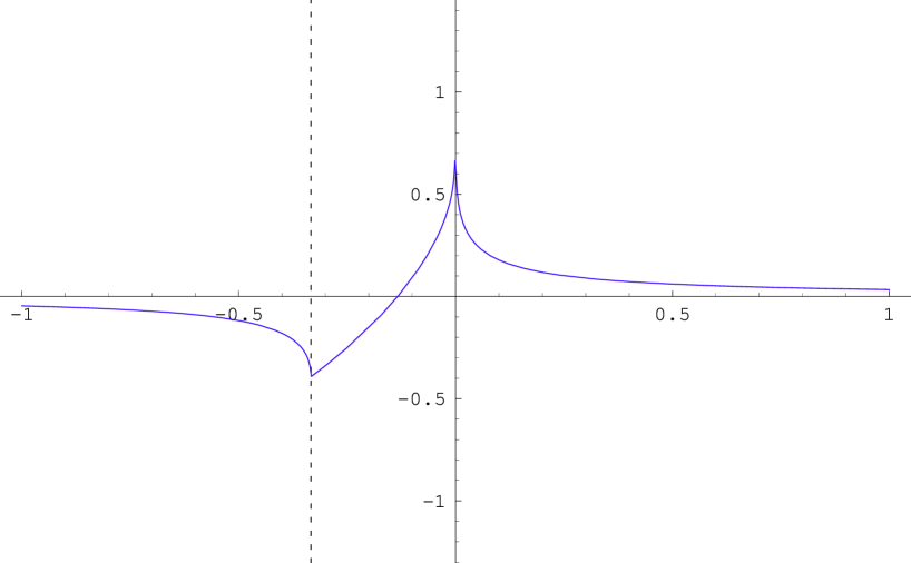
Figure 1: $A_{ee}$ as a function of $\lambda$. The dashed line is at $\lambda=-1/3$.

Let us note a few key features. It seems that when $\lambda=1$, $A_{ee}$ is not well defined. However, careful analysis will show that in fact $A_{ee}$ is continuous there and

$$A_{ee}(\lambda=1)=-\frac{3}{4}V_{00}^{rr}+\frac{7\zeta(3)}{2\pi^{2}}$$

where $\zeta(z)$ is the celebrated Riemann $\zeta$-function.

Also despite the discontinuity of $\alpha(\lambda)$, $A_{ee}$ is well-defined at $\lambda=-1/3=M(k=0)$. We can compute both limits from the left and the right to obtain

$$A_{ee}(-\frac{1}{3})=-\frac{3}{4}V_{00}^{rr}=-\frac{3}{4}\ln\frac{27}{16}.$$ (58)

This incidentally proves the identity (12), which has so far escaped the literature. The reason for this good behaviour is that near $k=0$, ${\cal N}(k)\sim 1$, $\left\langle k\right|v_{e}\rangle\sim k$ and $\lambda-M(k)=-1/3-M(k)\sim k^{2}$, so the integrand is well defined. This is not true for $\lambda=0$ where $A_{ee}$ diverges as $\ln\ln(\lambda)$. In fact

$$A_{ee}(\lambda\rightarrow 0)\sim\frac{2\,\gamma+16\,\ln(2)-9\,\ln(3)-2\,\ln(2\,\pi)+2\,\ln(-\ln\left|\lambda\right|)}{4}$$

One root of $Det$ can be found by solving

$$A_{ee}=-\frac{3}{4}V_{00}^{rr}+b\left(\frac{1}{2(1-\lambda)}-\frac{3}{8}\right)\equiv I_{b}(\lambda)$$ (59)

By studying the intersection of $I_{b}(\lambda)$ with $A_{ee}(\lambda)$ we see that there are two kinds of roots (cf. Figure 2). We note that $I_{b}(\lambda)$ is a hyperbola with asymptote at $\lambda=1$ so from $-\infty$ to $1$ it is an increasing function from $-\frac{3}{4}\beta$ to $\infty$. Therefore the first kind of root exists no matter what $b$ is (we recall that $b>0$), namely they are $\lambda=-1/3$ (because $I_{b}$ always passes through the point $(-1/3,-3/4\ln(27/16))\sim(-1/3,-0.392436)$, the left cusp point of $A_{ee}$; we will show this below) and some $\lambda_{1}\in(0,1)$. However when $I_{b}$ increases fast enough, it could intersect $A_{ee}$ one more time in the region $[-1/3,0)$; this is when $\frac{dI_{b}}{d\lambda}|_{-1/3}\geq\frac{dA_{ee}}{d\lambda}|_{-1/3}$. So the critical point occurs at $\frac{dI_{b}}{d\lambda}|_{-1/3}=\frac{dA_{ee}}{d\lambda}|_{-1/3}\Rightarrow b=8\ln 2$. Therefore a second kind of root exists in addition to the first only when $b\geq 8\ln 2$ and is located in the region $[-1/3,0)$.

As promised, we will now show that indeed $\lambda=-1/3=M(k=0)$ gives $1-\frac{4(\lambda-1)}{3\beta(1-\lambda)-2b}A_{ee}=0$. To see this, we recall from (58) that $A_{ee}(\lambda=-\frac{1}{3})=-\frac{3}{4}V_{00}^{rr}$. Using this we can calculate

$$1-\frac{4(\lambda-1)}{3\beta(1-\lambda)-2b}A_{ee}=1-\frac{4(-1/3-1)}{3(V_{00}^{rr}+b/2)(1+1/3)-2b}(-\frac{3}{4})V_{00}^{rr}=0.$$

We see therefore that $I_{b}(\lambda)$ passes through the left cusp of $A_{ee}(\lambda)$ and $\lambda=-\frac{1}{3}$ indeed is a root of $Det$.

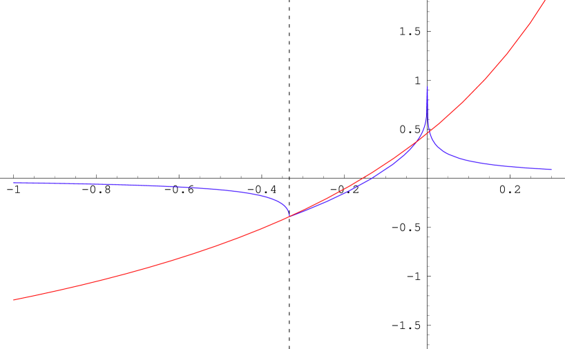
Figure 2: The intersection of $A_{ee}$ with $I_{b}$ as functions of $\lambda$. We have here chosen a $b$ above the critical value $b_{0}$ so that we can explicitly see 3 points of intersection. Note that both $A_{ee}$ and $I_{b}$ always meet at least at the dashed line at $\lambda=-1/3$.

5.2 The Function $A_{oo}$

By the same method we can evaluate

$$A_{oo}(\lambda):=\int_{-\infty}^{\infty}{dt\over t}{3\sinh(t)\over 2\left(1+2\cosh(t)\right)\left(1+\lambda+2\lambda\cosh(t)\right)}.$$

Now we obtain

$$A_{oo}(\lambda)={3\over 4}\left(\begin{array}[]{c}\\ \\ \end{array}2\gamma+3\ln 3+\psi\left[1+g(\lambda)\right]+\psi\left[1-\alpha(\lambda)-g(\lambda)\right]\right),$$

where $g(\lambda)$ and $\alpha(\lambda)$ were defined in (57).

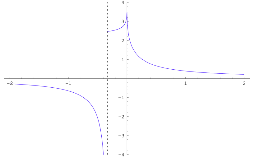
Figure 3: $A_{oo}$ as a function of $\lambda$. The dashed line is at $\lambda=-1/3$.

We plot $A_{oo}$ in Figure 3. There are several important points here as well. Firstly putting $\lambda=1$ we get $\langle v_{o}|\frac{1}{1-M}\left|v_{o}\right\rangle=\frac{3}{4}V_{oo}^{rr}$, giving us the nice identity. Secondly $A_{oo}$ diverges at $\lambda=0$ from both sides. The divergence is again very slow, as $\ln\ln\lambda$:

$$A_{oo}(\lambda\rightarrow 0)\sim\frac{3\,\left(2\,\gamma+3\,\ln(3)-2\,\ln(2\,\pi)\right)}{4}+\frac{3\,\ln(-\ln(\left|\lambda\right|))}{2}$$

More important is the behavior near $\lambda=-1/3$. If we approach from the left we find $A_{oo}|_{(-\frac{1}{3})^{-}}=-\infty$. If we approach from the right, we find $A_{oo}|_{(-\frac{1}{3})^{+}}=\frac{3}{4}\ln 27$ which is finite. This discontinuity may seem unnatural, but we will see later that it is consistent with our analysis.

Now we can solve the other $\lambda$ which makes $Det$ zero. The equation is

$$A_{oo}=\frac{3\beta}{4}=\frac{3}{4}\left(\ln\frac{27}{16}+\frac{b}{2}\right).$$ (60)

From this we find again that there are two kinds of solutions. The first one does not depend on the value of $b$ and is located in the region $(0,1)$ (since $b>0$). For large enough $b$, of course, we obtain a second type of zero in addition to the first, located in the region $[-1/3,0)$. This occurs when the right hand side is higher than when $A_{oo}$ takes its point of discontinuity at $\lambda=-1/3$; this is when $b\geq 8\ln 2$. Comparing with the critical value of $b$ found in the $A_{ee}$ case, we find they are same. This is not an accident.

In fact we claim that the solutions $\lambda$ found in both cases, either from $A_{ee}$ or from $A_{oo}$, whether in the region $(0,1)$ or $[-1/3,0)$ are the same, i.e., the two roots of $Det$ are degenerate. To show this, we use the analytic form of $A_{ee}$ and $A_{oo}$, giving the ratio

$$\frac{1-\frac{4}{3\beta}A_{oo}}{1-\frac{4(\lambda-1)}{3\beta(1-\lambda)-2b}A_{ee}}=\frac{b+3b\lambda+6(\lambda-1)\ln\left({27\over 16}\right)}{(1+3\lambda)\left(b+2\ln\left({27\over 16}\right)\right)}.$$ (61)

As analysed, the denominator gives one root of $Det$ and the numerator, the other. The idea is that if the roots are degenerate, they will cancel each other so that this ratio is neither zero nor infinite at the roots. From (61) we see that the ratio is zero only when $\lambda=(6\ln(27/16)-b)/(3b+6\ln(27/16))$; careful analysis reveals that this zero is coming from the simple pole in the denominator at $3\beta(1-\lambda)-2b=0$ and so is in fact not a zero of $Det$. On the other hand, the only pole is at $\lambda=-1/3$. We hence conclude that the two zeros of $Det$ are degenerate except for $\lambda=-\frac{1}{3}$ which is a zero of the denominator only (for all values of $b$).

6 The Discrete Spectrum

Having discussed the continuous spectrum, we now move on to the discrete spectrum. This comes from the zeros of the determinant $Det$. The solutions have been discussed in section 5. In this section, we will construct the corresponding eigenvectors.

6.1 The Case of $\lambda=-1/3$

As we have shown, no matter what $b$ is, $M_{ee}=1-\frac{4(\lambda-1)}{3\beta(1-\lambda)-2b}A_{ee}=0$ always has a solution $\lambda=-1/3$. We will denote the corresponding eigenvector as $v_{+,-\frac{1}{3}}$. Furthermore, when $b\geq 8\ln 2$, both $M_{ee}$ and $M_{oo}=1-\frac{4}{3\beta}A_{oo}$ have another solution $\lambda\in[-1/3,0)$. When $b=8\ln 2$, the solution will be $\lambda=-1/3$ again, which is also degenerate.

Now we can start to construct the eigenvectors. Since $M_{ee}=0$, for consistency of (38), we need $B_{e}=0$. This can be achieved by choosing any $k_{0}\neq 0$ or $k_{0}=0$ such that $r(k=0)/(-\frac{1}{3}-M(k=0))$ is not a pole.

If we choose $k_{0}\neq 0$, we have $B_{o}=0$ and the solution is

$${\cal C}_{e}=\frac{2V_{oo}^{rr}}{\sqrt{2b}},~{}~{}~{}~{}~{}~{}~{}{\cal C}_{o}=0$$ (62)

and the eigenvector becomes

$$g = 1,$$

$$\int_{-\infty}^{+\infty}dkh(k)\left|k\right\rangle = \int_{-\infty}^{+\infty}dk\left(-\frac{8}{3\sqrt{2b}}\frac{\left|k\right\rangle\left\langle k\right|v_{e}\rangle}{{\cal N}(k)(-1/3-M(k))}\right)$$

$$= -\frac{8}{3\sqrt{2b}}\frac{1}{(-1/3-M)}\left|v_{e}\right\rangle$$

$$= \frac{8}{\sqrt{2b}}\frac{1}{1+3M}\left|v_{e}\right\rangle.$$

In summary then,

$$v_{+,-\frac{1}{3}}=\left[\begin{array}[]{c}1\\ \frac{8}{\sqrt{2b}}\frac{1}{1+3M}\left|v_{e}\right\rangle\end{array}\right]$$ (63)

which is the solution given in [12] (equation (4.5)). Notice that this state is twist-even. This solution has been found by several groups already [17, 12, 20].

If instead of choosing $k_{0}\neq 0$, we choose $k_{0}=0$ such that $r(k)/(-1/3-M(k))$ does not have a pole at $k=0$, then there are two cases. The first one is that $r(k)/(-1/3-M(k))$ has a zero at $k=0$, so we have $B_{o}=0$ and the solution is the same as above. The second one is that $r(k)/(-1/3-M(k))\sim 1$ at $k=0$, then we will have a non-zero $B_{o}$. We point out that this is when $b\neq b_{0}:=8\ln 2$. Indeed if $b=b_{0}$, consistency of (38) requires $Det$ and hence $B_{o}$ to be zero. This non-zero $B_{o}$ opens the possibility for another eigenvector. If we choose the branch $A_{oo}|_{(-\frac{1}{3})^{-}}=-\infty$, we will have ${\cal C}_{o}=0$ although $B_{o}\neq 0$. However, if we choose the branch $A_{oo}|_{(-\frac{1}{3})^{+}}=\frac{3}{4}\ln 27$, we get a nonzero ${\cal C}_{o}$. In this case we can construct two eigenvectors: one is twist-even and one is twist odd.

Let us work out the details. Setting $k_{0}=0$ and expanding around $k=0$ we obtain $(-1/3-M(k))\sim k^{2}+O(k^{3})$ (the first order is zero). Therefore we can choose the parametre $r(k)=k^{2}$ and get $B_{o}=-6\sqrt{3}/\pi$. Then ${\cal C}_{o}=-\frac{6\sqrt{3}}{\pi(1-\frac{\ln 27}{\beta})}$. If we set ${\cal C}_{e}=0$, we get the eigenvector as

$$v_{-,-\frac{1}{3}}=\left[\begin{array}[]{c}0\\ \frac{4{\cal C}_{o}}{3\beta}\frac{1}{-1/3-M}\left|v_{o}\right\rangle-\frac{36}{\pi^{2}}\left|k=0\right\rangle\end{array}\right].$$ (64)

We can check this directly by acting $M^{\prime}$ on the left. Using

$$\left\langle v_{e}\right|k=0\rangle=0,\quad\left\langle v_{e}\right|\frac{1}{-1/3-M}\left|v_{o}\right\rangle=0,\quad\left\langle v_{o}\right|k=0\rangle=\frac{\sqrt{3}\pi}{6},\quad A_{oo}|_{(-\frac{1}{3})^{+}}=\frac{3}{4}\ln 27.$$

If we choose ${\cal C}_{e}=\frac{2V_{oo}^{rr}}{\sqrt{2b}}$, we will get

$$v^{\prime}=\left[\begin{array}[]{c}1\\ \frac{8}{\sqrt{2b}}\frac{1}{1+3M}\left|v_{e}\right\rangle+\frac{4{\cal C}_{o}}{3\beta}\frac{1}{-1/3-M}\left|v_{o}\right\rangle-\frac{36}{\pi^{2}}\left|k=0\right\rangle\end{array}\right].$$

From these two solutions we can construct the twist-odd solution $v_{-,-\frac{1}{3}}$ and the twist-even solution $v_{+,-\frac{1}{3}}=v^{\prime}-v_{-,-\frac{1}{3}}$, which is equal to (64). In fact, comparing with the results (48) and (49) from the last section, we find that these two solution $v_{\pm,-\frac{1}{3}}$ are nothing new, but a part of the continuous spectrum we presented before.

It is a little strange that we get twist-even and twist-odd states for $M^{\prime}$ at $\lambda=-1/3$ at the same time while for $M$, we have only a twist-odd state. To see that it is true, let us take $b\rightarrow+\infty$. In this limit we have from (9)

$$M^{\prime}=\left[\begin{array}[]{cc}-\frac{1}{3}&0\\ 0&M\end{array}\right].$$

From this limit, we see immediately that $M^{\prime}$ has two eigenvectors for the eigenvalue $-\frac{1}{3}$:

$$v_{+}=\left[\begin{array}[]{c}1\\ 0\end{array}\right],~{}~{}~{}~{}~{}~{}v_{-}=\left[\begin{array}[]{c}0\\ \left|k=0\right\rangle\end{array}\right];$$

these are of course nothing other than the limit of $v_{\pm,-\frac{1}{3}}$ when $b\rightarrow+\infty$. We consider this as a strong evidence supporting the double degeneracy at $\lambda=-1/3$. In the conclusions section, we will give some numerical evidence and further discussion about this point.

We have discussed the case of $b\neq b_{0}$ in the above and found that the discrete spectrum at $\lambda=-1/3$ is the same as the continuous at this point. Now we discuss the special case when $b=b_{0}=8\ln 2$. Recall from Subsection 5.2, we must choose the branch of $A_{oo}|_{(-\frac{1}{3})^{+}}=\frac{3}{4}\ln 27$ in order to get a zero for the determinant. Consistency of (38) requires $B_{e}=B_{o}=0$. This can be achieved by setting $k_{0}\neq 0$ or by setting $k_{0}=0$ but with $r(k)/(-1/3-M(k))$ having a zero at $k=0$. In either choice we will get two eigenvectors by letting ${\cal C}_{e}\neq 0,~{}~{}{\cal C}_{o}=0$ or ${\cal C}_{e}=0,~{}~{}{\cal C}_{o}\neq 0$. The results are

$$v^{b_{0}}_{+,-\frac{1}{3}}=\left[\begin{array}[]{c}1\\ \frac{8}{\sqrt{2b}}\frac{1}{1+3M}\left|v_{e}\right\rangle\end{array}\right]$$ (65)

and

$$v^{b_{0}}_{-,-\frac{1}{3}}=\left[\begin{array}[]{c}0\\ \frac{4{\cal C}_{o}}{3\beta}\frac{1}{-1/3-M}\left|v_{o}\right\rangle\end{array}\right].$$ (66)

Notice that although $v^{b_{0}}_{+,-\frac{1}{3}}$ is the same as (63), $v^{b_{0}}_{-,-\frac{1}{3}}$ is different from (64) by missing the $\left|k=0\right\rangle$ term. This is a very important point. It in fact distinguishes the continuous and the discrete spectra. This means that when $b_{0}\neq 8\ln 2$, the continuous spectrum at $\lambda=-1/3$ is simply the discrete spectrum at this point. However when $b_{0}=8\ln 2$, the expressions (48) and (49) for the continuous spectrum at $\lambda=-1/3$ no longer apply but should be replaced by (65) and (66).

6.2 Other Solutions at $\lambda\neq-1/3$

For other $\lambda\neq-1/3$ which make $Det$ zero no matter which region they are, the eigenvectors can be found similarly. First we choose ${\cal C}_{e}\neq 0,~{}~{}{\cal C}_{o}=0$ and the eigenvector is twist even

$$v_{+}=\frac{1}{2}(v(k_{0})+v(-k_{0}))=\left[\begin{array}[]{c}\frac{2\sqrt{2b}}{3\beta(1-\lambda)-2b}{\cal C}_{e}(k_{0})\\ \frac{4(\lambda-1)}{3\beta(1-\lambda)-2b}{\cal C}_{e}(k_{0})\frac{1}{\lambda-M}\left|v_{e}\right\rangle\end{array}\right].$$ (67)

Next we choose ${\cal C}_{e}=0,~{}~{}{\cal C}_{o}\neq 0$ and the eigenvector is twist odd

$$v_{-}=\frac{1}{2}(v(k_{0})-v(-k_{0}))=\left[\begin{array}[]{c}0\\ \frac{4}{3\beta}{\cal C}_{o}(k_{0})\frac{1}{\lambda-M}\left|v_{o}\right\rangle\end{array}\right].$$ (68)

Again, when $\lambda\in[-1/3,0)$ the expressions (48) and (49) for the continuous spectrum will be replaced by these above expressions for the discrete spectrum.

7 The Generating Function

In the above sections, we have given the eigenvectors of $M^{\prime}$ for the various ranges of $\lambda$. They are of the form of $\left|v_{e}\right\rangle$ and $\left|v_{o}\right\rangle$ acted on by ${1\over\lambda-M}$. It would be very nice if we could explicitly determine these components. The present section solves this problem.

In order to find components, we need to find the generating function. The idea is that, recalling $f_{k}$ in (4) we can define generating functions $G_{e}(z)$ and $G_{o}(z)$ as follows:

$$G_{e}(z)\equiv\left\langle z\right|E^{-1}\frac{1}{\lambda-M}\left|v_{e}\right\rangle = \int_{-\infty}^{+\infty}dk{f_{k}(z)\left\langle k\right|v_{e}\rangle\over{\cal N}(k)(\lambda-M(k))},$$ (69)

$$G_{o}(z)\equiv\left\langle z\right|E^{-1}\frac{1}{\lambda-M}\left|v_{o}\right\rangle = \int_{-\infty}^{+\infty}dk{f_{k}(z)\left\langle k\right|v_{o}\rangle\over{\cal N}(k)(\lambda-M(k))}.$$ (70)

The series expansion coefficients in $z$ of $G_{e}(z)$ (respectively $G_{o}(z)$) will give the components of ${1\over\lambda-M}\left|v_{e}\right\rangle$ (respectively ${1\over\lambda-M}\left|v_{o}\right\rangle$).

Recalling the definition of $f_{k}$ in (4), as well as (4) and (5), in addition to (3) and (7), the integrals have the explicit forms

$$G_{e}(z) = \int_{-\infty}^{+\infty}dk\frac{\left(1-e^{-k\arctan z}\right)\,\left(-1+\cosh(\frac{k\,\pi}{2})\right)\,}{2\,k\,\left(1+2\,\cosh(\frac{k\,\pi}{2})\right)\,\left(\lambda+\frac{1}{1+2\,\cosh(\frac{k\,\pi}{2})}\right)\sinh(\frac{k\,\pi}{2})}$$ (71)

$$G_{o}(z) = \int_{-\infty}^{+\infty}dk\frac{{\sqrt{3}}\,\left(1-e^{-k\arctan z}\right)}{2\,k\,\left(1+2\,\cosh(\frac{k\,\pi}{2})\right)\,\left(\lambda+\frac{1}{1+2\,\cosh(\frac{k\,\pi}{2})}\right)}$$ (72)

Our task is therefore to evaluate the above two integrals. Again summing up the residues on the upper half plane we obtain the following.

7.1 The Twist-even States

For the generating function $G_{e}(z)$, when $\lambda\in[-1/3,0)$, setting $\lambda=-(2\cosh(\frac{\pi k_{0}}{2})+1)^{-1}$ we have

$$G_{e}(z) = {1+2\cosh({\pi k_{0}\over 2})\over 4k_{0}(1+\cosh({\pi k_{0}\over 2}))}\left(k_{0}B[e^{-4i\arctan z};1-{ik_{0}\over 4},0]+k_{0}B[e^{-4i\arctan z};1+{ik_{0}\over 4},0]\right.$$ (73)

$$\left.+k_{0}(2\gamma-4{\rm arctanh}(e^{-2i\arctan z})+\ln(16)+\psi(-{ik_{0}\over 4})+\psi({ik_{0}\over 4}))-4i\sinh(k_{0}\arctan z)\right)$$

where

$$B[z;a,b]\equiv B_{z}[a,b]=\int\limits_{0}^{z}t^{a-1}(1-t)^{b-1}dt$$

for $(\mathop{\rm Re}(a)>0)$ is the incomplete beta function.

For $\lambda_{1}\in(0,1)$ we set

$$\lambda_{1}=(2\cosh(\frac{\pi k_{0}}{2})-1)^{-1}$$ (74)

and have

$$G_{e}(z) = {i(-1+2\cosh({\pi k_{0}\over 2})){\rm csch}^{2}({\pi k_{0}\over 4})\over 2}\left(i{\rm arctanh}(e^{-2i\arctan z})\begin{array}[]{c}\\ \\ \end{array}\right.$$ (78)

$$-{i\over 4}\left(2\gamma+\ln(16)+\psi({1\over 2}-{ik_{0}\over 4})+\psi({1\over 2}+{ik_{0}\over 4})\right)$$

$$+{e^{-(k_{0}+2i)\arctan z}\over 2i+k_{0}}~{}_{2}F_{1}[{1\over 2}-{ik_{0}\over 4},1,{3\over 2}-{ik_{0}\over 4},e^{-4i\arctan z}]$$

$$\left.+{e^{(k_{0}-2i)\arctan z}\over 2i-k_{0}}~{}_{2}F_{1}[{1\over 2}+{ik_{0}\over 4},1,{3\over 2}+{ik_{0}\over 4},e^{-4i\arctan z}]\right)$$

where

$${}_{2}F_{1}[a,b,c,z]={\Gamma(c)\over\Gamma(b)\Gamma(c-b)}\int\limits_{0}^{1}t^{b-1}(1-t)^{c-b-1}(1-tz)^{-a}dt$$

(for $\mathop{\rm Re}(c)>\mathop{\rm Re}(b)>0;|{\rm Arg}(1-z)|\leq\pi$) is the hypergeometric function of the first kind.

As an application of the above generating function, we derive the components of the state $v_{+,-{1\over 3}}$ in (64). Taking the limit $\lambda\rightarrow-1/3$ (or equivalently $k_{0}\rightarrow 0$) we can simplify the generating function $G_{e}(z)$ as

$$G_{e}(z)|_{k_{0}=0} = {3\over 4}\ln(1+z^{2})$$ (79)

$$= -{3\over 4}\sum_{n\geq 1}\frac{(-)^{n}}{n}z^{2n}=-{3\over 2}\sum_{k=even}\frac{1}{\sqrt{k}}\frac{(-)^{k/2}}{\sqrt{k}}z^{k}.$$ (80)

We conclude therefore that (up to an overall factor) the twist-even eigenvector at $\lambda=-1/3$ (from (63)) has components

$$v_{k}=\frac{4}{\sqrt{2b}}\frac{(-1)^{k/2}}{\sqrt{k}}\quad\mbox{$k$ even and }>0,$$

$v_{0}=1$ and $v_{k}=0$ for $k$ odd. This reproduces the result given in equation (4.15) of [17] for $b=4$.

7.2 The Twist-odd States

Now we discuss the generating function $G_{o}(z)$. Again, when $\lambda\in[-1/3,0)$ we can set $\lambda=-1/(2\cosh(\pi k_{0}/2)+1)$ and obtain

$$G_{o}(z) = {\sqrt{3}(2\coth({\pi k_{0}\over 2})+{\rm csch}({\pi k_{0}\over 2}))\over 4}\left(B[e^{-4i\arctan z};1-{ik_{0}\over 4},0]-B[e^{-4i\arctan z};1+{ik_{0}\over 4},0]\right.$$ (81)

$$\left.\qquad\qquad+{4i\cosh(k_{0}\arctan z)\over k_{0}}-i\pi\coth({\pi k_{0}\over 4})\right).$$

On the other hand, when $\lambda_{1}\in(0,1)$ we can set $\lambda_{1}=1/(2\cosh(\pi k_{0}/2)-1)$ and obtain

$$G_{o}(z) = \frac{i\sqrt{3}(-1+2\cosh({\pi k_{0}\over 2})){\rm csch}({k_{0}\pi\over 2})}{8k_{0}}\left(-i(k_{0}-2i)B[e^{-4ia},{1\over 2}-{ik_{0}\over 4},0]\right.$$ (82)

$$+e^{-2(4i+k_{0})a}\left({4e^{(6i+k_{0})a}(-2i+k_{0}+2e^{2k_{0}a}k_{0})\over k_{0}-2i}~{}_{2}F_{1}[1,{1\over 2}+{ik_{0}\over 4},{3\over 2}+{ik_{0}\over 4},e^{-4ia}]\right.$$

$$-2e^{(k_{0}+2i)a}\left({8i\over k_{0}+6i}~{}_{2}F_{1}[2,{3\over 2}-{ik_{0}\over 4},{5\over 2}-{ik_{0}\over 4},e^{-4ia}]\right.$$

$$\left.\left.\left.+{8i\over k_{0}-6i}~{}_{2}F_{1}[2,{3\over 2}+{ik_{0}\over 4},{5\over 2}+{ik_{0}\over 4},e^{-4ia}]+e^{(k_{0}+6i)a}k_{0}\pi\tanh({k_{0}\pi\over 4})\right)\right)\right)\,,$$

where $a\equiv\arctan z$.

As an application, we now try to find the components of $v_{-,-{1\over 3}}$. This is the twist-odd eigenvector at eigenvalue $\lambda=-1/3$ whose existence is so-far unpredicted. As we have mentioned, this state exists only when we reach $\lambda=-1/3$ from the right hand side. This corresponding to $k_{0}\rightarrow 0$ and we find the limit

$$G_{o}(z)|_{-({1\over 3})^{+}} = {i\sqrt{3}\over 8\pi}[24(\arctan z)^{2}-\pi^{2}+6\ln(e^{-4i\arctan z})\ln(1-e^{-4i\arctan z})+6{\rm Li}_{2}[e^{-4i\arctan z}]]$$ (83)

$$= {3\sqrt{3}z\over\pi}-{7z^{3}\over\sqrt{3}\pi}+{43\sqrt{3}z^{5}\over 25\pi}-{337\sqrt{3}z^{7}\over 245\pi}+{1091z^{9}\over 315\sqrt{3}\pi}+...$$

where ${\rm Li}_{2}[z]=\sum\limits_{k=1}^{\infty}z^{k}/k^{2}$ (for $|z|<1$) is the dilogarithm function.

8 The spectrum of $M^{\prime 12}$ and $M^{\prime 21}$

We digress here for a moment to present another application of our analysis. Knowing the spectrum of $M^{{}^{\prime}11}\equiv M^{\prime}$ it is easy to calculate that of the matrices ${M^{\prime}}^{12}$ and ${M^{\prime}}^{21}$.

The method is in direct parallel to the discussions in [9] because the matrices ${M^{\prime}}^{rs}$ obey the same useful properties as the matrices $M^{rs}$:

$$[{M^{\prime}}^{rs},{M^{\prime}}^{r^{\prime}s^{\prime}}]=0\quad\forall r,s,r^{\prime},s^{\prime}=1,2,3$$ (84)

$${M^{\prime}}+{M^{\prime}}^{12}+{M^{\prime}}^{21}=(M^{\prime})^{2}+({M^{\prime}}^{12})^{2}+({M^{\prime}}^{21})^{2}=1\quad,\quad{M^{\prime}}^{12}{M^{\prime}}^{21}=M^{\prime}(M^{\prime}-1)\,.$$ (85)

From (84), we see that all ${M^{\prime}}^{rs}$ share the same eigenvectors. The continuous eigenvalues $\lambda^{12}(k)$ and $\lambda^{21}(k)$ of ${M^{\prime}}^{12}$ and ${M^{\prime}}^{21}$ respectively, can then be calculated by treating (85) as a system of equations in $\lambda^{rs}(k)$. We thus obtain:

$$\lambda^{12}(k)-\lambda^{21}(k) = \pm\sqrt{(1-\lambda(k))(1+3\lambda(k))}$$ (86)

$$\lambda^{12}(k)+\lambda^{21}(k) = 1-\lambda(k)\,.$$ (87)

Because in the limit $b\rightarrow\infty$, ${M^{\prime}}^{12}$ and ${M^{\prime}}^{21}$ have similar diagonalized form as $M^{\prime}$, we should obtain the same eigenvalues as for the matrices $M^{rs}$. We can extend the choice of sign in front of the square root (from [9]) to finite values of $b$. We therefore have, for the continuous spectrum,

$$\lambda^{12}(k) = {1\over 2}{\rm sign}(k)\sqrt{(1-\lambda(k))(1+3\lambda(k))}+{1\over 2}(1-\lambda(k))$$ (88)

$$\lambda^{21}(k) = -{1\over 2}{\rm sign}(k)\sqrt{(1-\lambda(k))(1+3\lambda(k))}+{1\over 2}(1-\lambda(k))\;.$$ (89)

Furthermore the doubly degenerate eigenvalue $\lambda_{1}$ of $M^{\prime}$ gives rise to the following 2 eigenvalues:

$$\lambda_{1+}^{12}=\lambda_{1+}^{21}\equiv\lambda_{1+} = {1\over 2}\sqrt{(1-\lambda_{1})(1+3\lambda_{1})}+{1\over 2}(1-\lambda_{1})$$ (90)

$$\lambda_{1-}^{12}=\lambda_{1-}^{21}\equiv\lambda_{1-} = -{1\over 2}\sqrt{(1-\lambda_{1})(1+3\lambda_{1})}+{1\over 2}(1-\lambda_{1})\,.$$ (91)

Because $\lambda_{1}\in(0,1)$, we have that $\lambda_{1+}\in(0,1)$ and $\lambda_{1-}\in\left(-{1\over 3},0\right)$.

9 Discussions and Conclusions

In this paper, we solved the eigenvalue and eigenvector problem for the matrix $M^{\prime}$. We found that its spectrum is composed of a continuous spectrum, which is the same as the spectrum of $M$, and a new discrete spectrum, which always contains an eigenvalue $\lambda_{1}$ in the range $(0,1)$. We obtained the closed form for all the eigenvectors and found that, for every eigenvalue (including $-{1\over 3}$), we have always one twist-even state and one twist-odd state.

A particular thing that we found is that there is a critical value $b_{0}=8\ln 2$ above which one pair of eigenvectors in the continuous spectrum is replaced by one pair of eigenvectors in the discrete spectrum, although the eigenvalue does not change. As the parameter $b$ is claimed to be irrelevant to the physics[2, 23], it would be interesting to understand the meaning of this critical value $b_{0}$.

The main difference between the spectrum of $M^{\prime}$ and that of $M$ is that the eigenvalue $-{1\over 3}$ is now doubly degenerate, and that we have one new doubly degenerate eigenvalue in the interval $(0,1)$. As we mentioned in Section 6, the double degeneracy at $\lambda=-{1\over 3}$ is a little mysterious although we have several pieces of evidence to support it. This degeneracy is a surprising result of our analysis. Indeed, in the light of [26, 20] it seems to mean that we now would have two commuting coordinates in the Moyal product decomposition of the star product. It is thus worth looking closer at our twist-odd eigenvector $v_{-,-{1\over 3}}$.

Let us try to see if level truncation can help us decide if $v_{-,-{1\over 3}}$ really is an eigenvector. For this we define $w(b,L)=-3M^{\prime}v_{-,-{1\over 3}}(b)$, where $M^{\prime}$ and $v_{-,-{1\over 3}}$ are truncated to level $L$. If $v_{-,-{1\over 3}}$ is an eigenvector of $M^{\prime}$ with eigenvalue $-{1\over 3}$, we expect that $w(b,L\rightarrow\infty)=v_{-,-{1\over 3}}(b)$ for any value of $b$. We show in the following table, the five first nonzero components of $w(b=1)$ at various levels of truncation, as well as their values extrapolated from a fit of the form $a_{0}+a_{1}/\log(L)+a_{2}/\log(L)^{2}+a_{3}/\log(L)^{3}$. In the last lines, we show their exact values as calculated from (83).

$L$	$w(b=1)_{1}$	$w(b=1)_{3}$	$w(b=1)_{5}$	$w(b=1)_{7}$	$w(b=1)_{9}$
100	0.119343	0.41301	-0.446308	0.43575	-0.416943
150	0.120588	0.447491	-0.487193	0.479292	-0.461839
200	0.121053	0.468778	-0.512582	0.506505	-0.490075
300	0.121347	0.49465	-0.543575	0.539889	-0.524878
400	0.121394	0.510341	-0.562439	0.560288	-0.546226
$\infty$	0.0984355	0.799035	-0.921314	0.962239	-0.980627
exact value	0.119946	0.608215	-0.681026	0.689616	-0.682686

Comparing the two last lines, we see that the result of the fit is about 20 to 40% away from the exact value. Though discouraging, this discrepancy is not conclusive because the fitting function might not be a judicious choice. Indeed note that the convergence is monotonic and very slow, and the values of the fit are surprisingly far away from our finite level values.

For comparison, we show in the next table $w_{+}(b,L)=-3M^{\prime}v_{+,-{1\over 3}}(b)$ for $b=1$ in the level truncation.

$L$	$w_{+}(b=1)_{0}$	$w_{+}(b=1)_{2}$	$w_{+}(b=1)_{4}$	$w_{+}(b=1)_{6}$	$w_{+}(b=1)_{8}$
100	0.874064	-1.86078	1.27486	-1.01287	0.855905
150	0.903461	-1.89268	1.30621	-1.04427	0.887334
200	0.920118	-1.91092	1.32429	-1.06252	0.905733
300	0.938883	-1.9316	1.34494	-1.08348	0.926978
400	0.949481	-1.94335	1.35673	-1.0955	0.939219
$\infty$	1.02072	-2.03708	1.46506	-1.2184	1.07553
exact value	1	-2	1.41421	-1.1547	1

We see that it converges towards the expected value much better than the $C$-odd vector does. We can try to compare this difference in numerical behavior to the case of the matrix $M$. Remember that in [9], the authors found a candidate $C$-even eigenvector (denoted $v^{+}$) of eigenvalue $-{1\over 3}$, in addition to the $C$-odd eigenvector $v^{-}$. This candidate was however discarded by the authors for several reasons:

• $v^{+}$ is an eigenvector of $K_{1}^{2}$ but not of $K_{1}$.

• The set of eigenvectors without $v^{+}$ already forms a complete basis [10].

• The norm of $v^{+}$ has a worse divergence than the norm of $v^{-}$.

• $v^{+}$ never appears in the level truncation.

Our analysis does not allow us to generalize these two first arguments to our case. But we can do the same level truncation tests as above with the vectors $v^{+}$ and $v^{-}$. In the following table, we show $u^{+}\equiv-3Mv^{+}$ at various truncations levels as well as the expected values.

$L$	$(u^{+})_{2}$	$(u^{+})_{4}$	$(u^{+})_{6}$	$(u^{+})_{8}$	$(u^{+})_{10}$
100	1.12259	-1.00375	0.90241	-0.822676	0.758504
150	1.1771	-1.06413	0.965334	-0.886898	0.823385
200	1.21013	-1.10103	1.00408	-0.926709	0.863861
300	1.24965	-1.14547	1.051	-0.975174	0.913374
400	1.27328	-1.17218	1.07933	-1.00457	0.943521
$\infty$	1.65594	-1.63066	1.58908	-1.55458	1.46357
$v^{+}$	1.41421	-1.33333	1.25196	-1.18525	1.13039

Now we compare this to the same analysis done with $u^{-}\equiv-3Mv^{-}$.

$L$	$(u^{-})_{1}$	$(u^{-})_{3}$	$(u^{-})_{5}$	$(u^{-})_{7}$	$(u^{-})_{9}$
100	0.957182	-0.531943	0.399565	-0.328769	0.283024
150	0.967172	-0.542301	0.410247	-0.33963	0.293974
200	0.97283	-0.548233	0.416417	-0.345949	0.300388
300	0.979205	-0.554972	0.423469	-0.353213	0.307799
400	0.982806	-0.558804	0.4275	-0.357384	0.312072
$\infty$	1.00694	-0.590333	0.46527	-0.400556	0.360073
$v^{-}$	1	-0.57735	0.447214	-0.377964	0.333333

We see that the difference in numerical behavior between $v_{-,-{1\over 3}}$ and $v_{+,-{1\over 3}}$ is qualitatively similar to the difference in numerical behavior between $v^{+}$ and $v^{-}$. This suggests that we should be suspicious about $v_{-,-{1\over 3}}$. The eigenstate indeed deserves further investigation. However, as we have shown in the limit $b\rightarrow\infty$, we do believe the existence of the state $v_{-,-{1\over 3}}$. We think that the reason why the level truncation does not work is that the components of $v_{-,-{1\over 3}}$ do not decay fast enough and level truncation is not very trustable in this case.

Let us move onto the other eigenvalues. The existence of the discrete eigenvalue $\lambda_{1}$ in the range $(0,1)$ can be considered as the result of us adding zero modes into the matrix $M$ to get $M^{\prime}$. This relationship may help us to understand the physical meaning of these discrete states. As a check, we can calculate the eigenvalues numerically in the level truncation scheme. We found that the eigenvalue in region $(0,1)$ converges very fast as the level is increased; this situation is very different from that for $\lambda=-{1\over 3}$ for example, which converges only logarithmically in level truncation [2, 9]. To illustrate this, we write in the following table the value of $\lambda_{1}$ at $b=0.2$, $b=1$ and $b=5$, found at various levels of truncation, as well as its exact values calculated from (59).

level 1 5 10 50 100 exact value $\lambda_{1}(b=0.2)$ 0.78606702 0.80099138 0.80260995 0.80326016 0.80328899 0.80329559 $\lambda_{1}(b=1)$ 0.39394374 0.40376417 0.40407525 0.40411239 0.40412026 0.40412740 $\lambda_{1}(b=5)$ 0.01082671 0.02795012 0.02859612 0.02873404 0.02873526 0.02873810

We see that, at level $10$, the relative error is less than $1\%$. And for $b=0.2$ and $b=1$, level $1$ is already a good approximation.

We hope that the results of this paper can find useful applications. In particular they should lead to some information about the instantonic sliver [18, 19]. Some future work could consist of seeking a better understanding of the density of eigenvalues in the continuous spectrum. Indeed, we have found no convincing argument to claim that it should be the same as for the matrix $M$. In fact, if those densities were the same, we could simplify the continuous spectrum between the numerator and the denominator of the ratio

$$R={T_{p}\over 2\pi\sqrt{\alpha^{\prime}}T_{p+1}}={3\left(V_{00}^{rr}+{b\over 2}\right)^{2}\over\sqrt{2\pi b^{3}}}{\det(1-M^{\prime})^{3\over 4}(1+3M^{\prime})^{1\over 4}\over\det(1-M)^{3\over 4}(1+3M)^{1\over 4}}\,.$$

But this would lead to a puzzle because $M^{\prime}$ has two eigenvectors with eigenvalue $-{1\over 3}$ (at least we think so), whereas $M$ has only one; $R$ would then naively be zero (and we know that it is one [12]).

As another direction for future research we can find the spectrum of the $M^{\prime}$ matrix in the presence of a background $B$-field in the vein of [24]. This will be addressed in a forthcoming work [25]. We can also discuss the relationship of the Moyal product with Witten’s star product in the case of including the zero modes as in [26].

References

- [1] L. Rastelli, A. Sen and B. Zwiebach, “String field theory around the tachyon vacuum,” arXiv:hep-th/0012251.
- [2] L. Rastelli, A. Sen and B. Zwiebach, “Classical solutions in string field theory around the tachyon vacuum,” arXiv:hep-th/0102112.
- [3] L. Rastelli, A. Sen and B. Zwiebach, “Half strings, projectors, and multiple D-branes in vacuum string field theory,” JHEP 0111, 035 (2001) [arXiv:hep-th/0105058].
- [4] L. Rastelli, A. Sen and B. Zwiebach, “Boundary CFT construction of D-branes in vacuum string field theory,” JHEP 0111, 045 (2001) [arXiv:hep-th/0105168].
- [5] L. Rastelli, A. Sen and B. Zwiebach, “Vacuum string field theory,” arXiv:hep-th/0106010.
- [6] D. Gaiotto, L. Rastelli, A. Sen and B. Zwiebach, “Ghost structure and closed strings in vacuum string field theory,” arXiv:hep-th/0111129.
- [7] L. Rastelli, A. Sen and B. Zwiebach, “A note on a proposal for the tachyon state in vacuum string field theory,” arXiv:hep-th/0111153.
- [8] E. Witten, “Noncommutative Geometry And String Field Theory,” Nucl. Phys. B 268, 253 (1986).
- [9] L. Rastelli, A. Sen and B. Zwiebach, “Star algebra spectroscopy,” arXiv:hep-th/0111281.
- [10] K. Okuyama, “Ghost kinetic operator of vacuum string field theory,” JHEP 0201, 027 (2002) [arXiv:hep-th/0201015].
- [11] H. Hata and T. Kawano, “Open string states around a classical solution in vacuum string field theory,” JHEP 0111, 038 (2001) [arXiv:hep-th/0108150].
- [12] K. Okuyama, “Ratio of tensions from vacuum string field theory,” arXiv:hep-th/0201136.
- [13] T. Okuda, “The equality of solutions in vacuum string field theory,” arXiv:hep-th/0201149.
- [14] L. Rastelli and B. Zwiebach, “Tachyon potentials, star products and universality,” JHEP 0109, 038 (2001) [arXiv:hep-th/0006240].
- [15] V. A. Kostelecky and R. Potting, “Analytical construction of a nonperturbative vacuum for the open bosonic string,” Phys. Rev. D 63, 046007 (2001) [arXiv:hep-th/0008252].
- [16] K. Furuuchi and K. Okuyama, “Comma vertex and string field algebra,” JHEP 0109, 035 (2001) [arXiv:hep-th/0107101].
- [17] G. Moore and W. Taylor, “The singular geometry of the sliver,” JHEP 0201, 004 (2002) [arXiv:hep-th/0111069].
- [18] D. J. Gross and W. Taylor, “Split string field theory. I,” JHEP 0108, 009 (2001) [arXiv:hep-th/0105059].
- [19] D. J. Gross and W. Taylor, “Split string field theory. II,” JHEP 0108, 010 (2001) [arXiv:hep-th/0106036].
- [20] Private communications with B. Zwiebach; also L. Rastelli, A. Sen, and B. Zwiebach, unpublished.
- [21] D. J. Gross and A. Jevicki, “Operator Formulation Of Interacting String Field Theory,” Nucl. Phys. B 283, 1 (1987).
- [22] D. J. Gross and A. Jevicki, “Operator Formulation Of Interacting String Field Theory. 2,” Nucl. Phys. B 287, 225 (1987).
- [23] P. Mukhopadhyay, “Oscillator representation of the BCFT construction of D-branes in vacuum string field theory,” JHEP 0112, 025 (2001) [arXiv:hep-th/0110136].
- [24] L. Bonora, D. Mamone and M. Salizzoni, “B field and squeezed states in vacuum string field theory,” arXiv:hep-th/0201060.
- [25] B. Feng, Y.-H. He and N. Moeller, to appear soon.
- [26] M. R. Douglas, H. Liu, G. Moore and B. Zwiebach, “Open String Star as a Continuous Moyal Product,” arXiv:hep-th/0202087.