[

String inspired braneworld cosmology

Abstract

We consider braneworld scenarios including the leading correction to the Einstein-Hilbert action suggested by superstring theory, the Gauss-Bonnet term. We obtain and study the complete set of equations governing the cosmological dynamics. We find they have the same form as those in Randall-Sundrum scenarios but with time-varying four-dimensional gravitational and cosmological constants. Studying the bulk geometry we show that this variation is produced by bulk curvature terms parameterized by the mass of a black hole. Finally, we show there is a coupling between these curvature terms and matter that can be relevant for early universe cosmology.

]

In recent decades developments in cosmology have been strongly influenced by high-energy physics. A remarkable example of this is the inflationary scenario and all its variants. This influence has been growing and becoming more and more important. Today it comes from developments in string and M theories and the new scenarios they are providing for cosmology. In particular, the study of scenarios where the spacetime has non-compact extra-dimensions has produced intense activity.

The most popular model of that class is the one proposed by Randall and Sundrum [1, 2] (RS), motivated by orbifold compactification of higher dimensional string theories, in particular, by the dimensional reduction of eleven-dimensional supergravity in ${\mathbb{R}}^{10}\times S^{1}/{\mathbb{Z}}_{2}$ introduced by Hořava and Witten [3]. The picture coming from the RS model is one with all matter and gauge fields, except gravity, confined in a three-brane embedded in a five-dimensional (5D) spacetime with ${\mathbb{Z}}_{2}$ symmetry, and where the zero-mode of the Kaluza-Klein (KK) dimensional reduction is localized, reproducing Newtonian gravity in the weak field approximation.

On the other hand, it is a general belief that Einstein gravity is a low-energy limit of a quantum theory of gravity which is still unknown. Among promising candidates we have string theory which suggests, that in order to have a ghost-free action, quadratic curvature corrections to the Einstein-Hilbert action must be proportional to the Gauss-Bonnet term [4]. This term also plays a fundamental role in Chern-Simons gravitational theories [5]. However, although being a string-motivated scenario, the RS model and its generalizations [6] do not include these terms. From a geometric point of view, the combination of the Einstein-Hilbert and Gauss-Bonnet term constitutes, for 5D spacetimes, the most general Lagrangian producing second-order field equations [7] (see also [8]).

These facts provide a strong motivation for the study of braneworld theories including a Gauss-Bonnet term. Recent investigations on this issue have shown [9] that the metric for a vacuum 3-brane (domain wall) is, up to a redefinition of constants, the warp-factor metric of the RS scenarios. The existence of a KK zero-mode localized on the 3-brane has also been demonstrated  [10] (see also [11, 12]). Properties of black hole solutions in AdS spacetimes have been studied in [13, 14]. The cosmological consequences of these scenarios are less well understood. This issue has been studied in [15, 16] in the case of a 2-brane model [1] and in [17] for a single-brane model [2]. However, in both cases only simple ansätze for the 5D metric (written in Gaussian coordinates as in [18]) were considered, e.g. the separability of the metric components in the time and extra-dimension coordinates. One can see that this assumption is too strong even in RS cosmological scenarios [18], where they lead to a very restrictive class of cosmological models, not representative of the true dynamics. Other works with higher-curvature terms in braneworld scenarios are considered in [19].

In this paper we obtain the equations governing the dynamics of Friedmann-Robertson-Walker (FRW) cosmological models in braneworld theories with a Gauss-Bonnet term. This includes the derivation of the appropriate junction conditions for this kind of theory. Then, we investigate the new dynamical cosmological behaviour and how it is related to the geometry of the bulk.

Our starting point is the following action

$$S = \frac{1}{\kappa^{2}}\int\!d^{5}x\sqrt{-g}\left({\cal L}_{EH}+\frac{\alpha}{2}{\cal L}_{GB}\right)$$ (2)

$$\hskip 56.9055pt+\int\!d^{4}x\sqrt{-\tilde{g}}\,\left({\cal L}_{m}-2\lambda\right)\,,$$

where ${\cal L}_{EH}=R-2\Lambda$ is the Einstein-Hilbert Lagrangian with a negative cosmological constant, $\Lambda<0$, ${\cal L}_{GB}$ is the Gauss-Bonnet correction

$${\cal L}_{GB}=R^{2}-4R^{AB}R_{AB}+R^{ABCD}R_{ABCD}\,,$$ (3)

and matter fields (${\cal L}_{m}$) are confined to a 3-brane with ${\mathbb{Z}}_{2}$ symmetry. Moreover, $\lambda$ is a constant that coincides with the brane tension in the limit ${\cal L}_{m}=0=\alpha$. Objects corresponding to the brane are written with a tilde to be distinguished from 5D objects; $g$ is the metric determinant and $R$, $R_{AB}$, and $R_{ABCD}$ are the scalar curvature and Ricci and Riemann tensors respectively; $\kappa$ is the 5D gravitational constant and physical units in which $c=1$ are assumed. The sign of the fundamental constant $\alpha$ must be positive according to the expansions carried out in string theory [4]. If we write the unit normal to the 3-brane as $\mbox{\boldmath$n$}=\mbox{\boldmath$dw$}$ (Gaussian coordinates), the field equations are

$$G_{AB}+\Lambda g_{AB}+\alpha H_{AB}=\kappa^{2}\left[-\lambda\tilde{g}_{AB}+T_{AB}\right]\delta(w)\,,$$ (4)

where $H_{AB}$ is the second-order Lovelock tensor [7]

$$H_{AB} = RR_{AB}-2R_{A}{}^{C}R_{BC}-2R^{CD}R_{ACBD}$$ (6)

$$+R_{A}{}^{CDE}R_{BCDE}-\textstyle{1\over 4}g_{AB}{\cal L}_{GB}\,,$$

$T_{AB}$ is the energy-momentum tensor describing the matter confined on the 3-brane ($T_{AB}n^{B}=0=\tilde{g}_{AB}n^{B}$). Since we are interested in the cosmological consequences of the theory we take $T_{AB}$ to be of the perfect-fluid type

$$T_{AB}=(\rho+p)u_{A}u_{B}+p\tilde{g}_{AB}\,,$$ (7)

with $u^{A}$, $\rho$, and $p$, being the fluid velocity ($u^{A}u_{A}=-1$), energy density and pressure respectively.

Homogeneous and isotropic cosmological models can be described by the 5D line element [18] ($i,j,\ldots=1,2,3$)

$$ds^{2}=-n^{2}(t,y)dt^{2}+a^{2}(t,y)h_{ij}dx^{i}dx^{j}+b^{2}(t,y)dy^{2}\,,$$ (8)

where $y$ is the fifth dimension coordinate (the brane is located at $y=0$) and $h_{ij}$ is a 3-dimensional maximally symmetric metric for the surfaces $\{t={\rm const.},y={\rm const.}\}$, whose spatial curvature is parameterized by $k=-1,0,1\,.$ Every hypersurface $y={\rm const.}$ has the metric of a FRW cosmological model.

The first step to solve the field equations (4) is to study them in the bulk ($y\neq 0$). Following [18] we have found that a set of functions $\{a(t,y),b(t,y),n(t,y)\}$ constitute a solution of the field equations in the bulk provided the following equations are satisfied [20]

$$\frac{\dot{a}}{a}\frac{n^{\prime}}{n}+\frac{a^{\prime}}{a}\frac{\dot{b}}{b}-\frac{\dot{a}^{\prime}}{a}=0\,,$$ (9)

$$\Phi+\alpha\Phi^{2}=\frac{\Lambda}{6}+\frac{C}{a^{4}}\,,$$ (10)

where $C$ is an integration constant and

$$\Phi(t,y)=\frac{1}{n^{2}}\frac{\dot{a}^{2}}{a^{2}}-\frac{1}{b^{2}}\frac{a^{\prime 2}}{a^{2}}+\frac{k}{a^{2}}\,.$$ (11)

The simplicity of equation (10) is remarkable and so is the fact that the Einstein-Hilbert and Gauss-Bonnet terms depend on the same argument, namely $\Phi\,.$ It would be interesting to know whether or not this happens also for higher-order terms in $D>5$ spacetimes, i.e., whether the dependence of the nth-order Lovelock term is of the form $\Phi^{n}$.

To find the equations for the 3-brane we need to study the junction conditions of our theory, which will be different from those in Einstein gravity [21]. We know that the 5D metric must be continuous across the brane and that there will be jumps in its normal derivatives due to the energy-momentum distribution on the brane [see Eq. (4)]. The ${\mathbb{Z}}_{2}$ symmetry makes the metric invariant under the transformation $y\rightarrow-y$ and hence any metric component can be written as $A(t,y)=\bar{A}(t,|y|)$. Therefore, the normal derivatives are given by

$$A^{\prime}(t,y)=\partial_{|y|}\bar{A}(t,|y|)\mbox{sign}(y)\equiv\bar{A}_{1}(t,|y|)\mbox{sign}(y)\,,$$ (12)

$$A^{\prime\prime}(t,y)=\partial_{|y|}\bar{A}_{1}(t,|y|)+2\bar{A}_{1}(t,|y|)\delta(y)\,.$$ (13)

The first derivative has a finite discontinuity across the brane but its square is continuous by virtue of the ${\mathbb{Z}}_{2}$ symmetry. The second derivative has a non-distributional part, the first term, and a distributional part whose coefficient gives the jump across the brane, namely $[A^{\prime}]=A^{\prime}(t,0^{+})-A^{\prime}(t,0^{-})=2\bar{A}_{1}(t,0)\,.$ The value of this jump can be obtained by integrating the tt-component of the field equations (4) across the brane, that is ($\delta(w)=b^{-1}_{o}\delta(y)$)

$$\lim_{\epsilon\rightarrow 0}\int^{\epsilon}_{-\epsilon}dy\left(G_{tt}+\Lambda g_{tt}+\alpha H_{tt}\right)=\kappa^{2}(\rho+\lambda)\frac{n^{2}_{o}}{b_{o}}\,,$$ (14)

where from now on the subscript “$o$” will denote the value of the corresponding quantity on the brane. Then, the equation for the jump $\bar{a}_{1}(t,0)$ is

$$\left[1+2\alpha\left(\frac{1}{n^{2}_{o}}\frac{\dot{a}^{2}_{o}}{a^{2}_{o}}-\frac{1}{b^{2}_{o}}\frac{\bar{a}^{2}_{1}}{a^{2}_{o}}+\frac{k}{a^{2}_{o}}\right)\right]\frac{\bar{a}_{1}}{a_{o}b_{o}}=-\frac{1}{6}(\lambda+\rho)\kappa^{2}\,.$$ (15)

This is a cubic equation for the discontinuity $\bar{a}_{1}$ which, for sufficiently small $\alpha$, has only one real solution, the other two being complex. Therefore, if we require our cosmological equations to have the right $\alpha\rightarrow 0$ limit we are left with only one solution. Introducing it into equation (10) will lead to the Friedmann equation for the brane. Equation (10) is a quadratic equation in the square of the Hubble function $H=\dot{a}_{o}/(n_{o}a_{o})$, but only one solution has the correct limit $\alpha\rightarrow 0$. Remarkably, the Friedmann equation we get from that solution can be written in the same form as in the RS cosmological scenario (compare with the generalized Friedmann equations in [22, 23])

$$H^{2}=\frac{1}{3}\tilde{\kappa}^{2}_{\ast}\rho\left(1+\frac{\rho}{2\lambda}\right)-\frac{k}{a^{2}_{o}}+\frac{1}{3}\tilde{\Lambda}_{\ast}\,,$$ (16)

where the 4D gravitational coupling and cosmological constants, $\tilde{\kappa}_{\ast}$ and $\tilde{\Lambda}_{\ast}$, are now time dependent. The only difference with the corresponding RS equation is that here we do not have explicitly the dark radiation term [22] proportional to $a^{-4}_{o}$. It is actually included, in a non-linear way, in $\tilde{\Lambda}_{\ast}$ [see Eq. (18) below]. The time-dependent fundamental “constants” $\tilde{\kappa}^{2}_{\ast}$ and $\tilde{\Lambda}_{\ast}$ change in time as functions only of the scale factor $a_{o}$. Their explicit form is

$$\tilde{\kappa}^{2}_{\ast} = \tilde{\kappa}^{2}\frac{1+\textstyle{2\over 3}\alpha\Lambda}{1+4\alpha\sigma}\,,~{}~{}\tilde{\kappa}^{2}\equiv\frac{\lambda\kappa^{4}}{6}\frac{1}{1+\textstyle{2\over 3}\alpha\Lambda}\,,~{}~{}\sigma\equiv\frac{\Lambda}{6}+\frac{C}{a^{4}_{o}}\,,$$ (17)

$$\tilde{\Lambda}_{\ast} = \frac{\lambda\tilde{\kappa}^{2}}{2}\frac{1+\textstyle{2\over 3}\alpha\Lambda}{1+4\alpha\sigma}-\frac{3}{2\alpha}\left(1-\sqrt{1+4\alpha\sigma}\right)\,,$$ (18)

where we have introduced $\sigma$, the function containing the dependence on $a_{o}$. Moreover, $\tilde{\kappa}^{2}$ is the 4D gravitational coupling constant, the one that appears in the computation of Newton’s law [11]. For small $\alpha$ we recover the Friedmann equation in RS braneworlds (see, e.g., [22, 23]). Actually, at zero order in $\alpha$, $\tilde{\Lambda}_{\ast}=\tilde{\Lambda}_{RS}+3Ca^{-4}_{o}+O(\alpha)\,,$ recovering the dark radiation term $Ca^{-4}_{o}$ in the Friedmann equation of RS brane-worlds.

The dependence of $\tilde{\kappa}^{2}_{\ast}$ and $\tilde{\Lambda}_{\ast}$ on $a_{o}$ has been plotted in Fig. 1. There are two possible behaviours according to whether $\tilde{\Lambda}_{\ast}$ has a minimum [Fig. 1(a)] or not [Fig. 1(b)]. In both cases $\tilde{\Lambda}_{\ast}$ tends to infinity for small $a_{o}$ and to a constant

$$\tilde{\Lambda}_{\infty}=\textstyle{{\lambda\tilde{\kappa}^{2}}\over 2}-\textstyle{3\over{2\alpha}}(1-\sqrt{1+\textstyle{2\over 3}\alpha\Lambda})\,,$$ (19)

when $a_{o}\rightarrow\infty$. Then, $\tilde{\Lambda}_{\ast}$ tends to zero for the following critical value of $\lambda$

$$\lambda_{c}=\textstyle{3\over{\alpha\tilde{\kappa}^{2}}}(1-\sqrt{1+\frac{2}{3}\alpha\Lambda})\,.$$ (20)

The case $\lambda=\lambda_{c}$, $\rho=C=k=0$ corresponds to a Minkowskian brane [1, 2] (see [9]). From Eq. (17) we must have $1+4\alpha\sigma>0$, hence from the behaviour for big and small $a_{o}$ we deduce that $\alpha|\Lambda|\leq 3/2$ and $\alpha C\geq 0$. On the other hand, the behaviour of $\tilde{\kappa}^{2}_{\ast}$, when $C\neq 0$, is the same independently of the value of the parameters; it tends to zero for small $a_{o}$ and to $\tilde{\kappa}^{2}$ [see Eq. (18)] when $a_{o}\rightarrow\infty\,.$

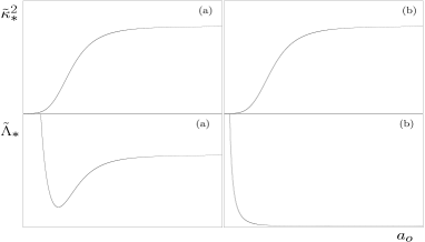
FIG. 1.: Variation of the effective 4D gravitational and cosmological constants, $\tilde{\kappa}^{2}_{\ast}$ and $\tilde{\Lambda}_{\ast}$, with respect to the scale factor $a_{o}$ [Eq. (18)]. (a) $\tilde{\Lambda}_{\ast}$ has a minimum. (b) $\tilde{\Lambda}_{\ast}$ is a monotonic function of $a_{o}$.

As in standard cosmology, the Friedmann equation (16) together with the energy-momentum tensor conservation equations [a consequence of the divergence-free character of the left-hand side of (4)],

$$\dot{\rho}=-3(\rho+p)H\,,$$ (21)

and a barotropic equation of state $p=p(\rho)$, describe completely the cosmological dynamics on the brane.

At this point we do not know much about the geometry of the bulk. For perfect-fluid FRW cosmological models in RS braneworlds, the bulk turns out to be the Schwarzschild-AdS 5D spacetime (see [24, 25]). Since in our case we have different gravitational equations [Eqs. (9, 10)] we do not expect the same bulk. The knowledge of the bulk geometry is important to understand the physical meaning of the integration constant $C$ appearing in the Friedmann equation (16,18). Assuming that the fifth dimension is static [18], $\dot{b}=0$, we have found that there is a coordinate change, analogous to the one used in RS scenarios [26], that brings the line element (8) to the following static form

$$ds^{2}=-f(R)dT^{2}+\frac{dR^{2}}{f(R)}+R^{2}(d\chi^{2}+\Sigma^{2}_{k}(\chi)d\Omega^{2}_{2})\,,$$ (22)

where $\Sigma_{-1}=\sinh\chi\,,$ $\Sigma_{0}=\chi\,,$ and $\Sigma_{1}=\sin\chi\,,$ and $d\Omega^{2}_{2}$ is the unit 2-sphere metric. In RS scenarios, Kraus [24] and Ida [25], found the Schwarzschild-${\rm AdS}_{5}$ bulk. When a Gauss-Bonnet is present, the solution of the field equations (4) for the line-element (22) is given by (see [4] for the $k=0$ case and [14] for any $k$)

$$f(R)=k+\frac{R^{2}}{2\alpha}\left(1-\sqrt{1+\frac{4\kappa^{2}\alpha M}{3V_{k}R^{4}}+\frac{2}{3}\alpha\Lambda}\right)\,,$$ (23)

where $V_{k}$ is the volume of the 3-surface $\{T={\rm const.},R=1\}$. In this picture, the 3-brane is a hypersurface that expands or contracts according to a law $R=R(T)$, where $R$ coincides with the scale factor, $R(T)=a(t,y)$, and $t$ is a proper time ($n_{o}=1$). More important, the constant $C$ is related to the black hole mass by the relation

$$C=\frac{\kappa^{2}M}{3V_{k}}\,.$$ (24)

Therefore, the string theory prediction that $\alpha$ must be positive implies, using $\alpha C\geq 0$, that the mass of the black hole must be positive. Conversely, if we require the avoidance of a naked singularity, $M>0$ [14], then the constant $\alpha$ must be positive.

As one would expect, if the mass of the black hole tends to zero the bulk Weyl tensor vanishes. This means that the effective time-variation of $\tilde{\kappa}^{2}_{\ast}$ is due to the coupling of bulk Weyl curvature terms with matter. From a geometrical point of view, it is a consequence of the structure of the curvature quadratic terms in the Gauss-Bonnet Lagrangian.

Let us now study what is the behaviour of FRW models in this theory. We start with the most simple case, when there is no black hole present in the bulk, which means $M=0$. In this case the dynamics is completely equivalent to that of RS braneworlds, widely discussed in the literature (see [23, 27] for an exhaustive study), where $\tilde{\kappa}$ and $\Lambda_{\infty}$ are the 4D gravitational and cosmological constants respectively. Moreover, one can check that in this case the conditions for inflation are the same as those described in [28].

To study the case $M\neq 0$ we assume a linear equation of state, $p=(\gamma-1)\rho$, which implies $\rho\propto a_{o}^{-3\gamma}\,.$ For late times, $a_{o}\gg 1$, and as in RS braneworlds, the behaviour is the same as in standard cosmology, $a_{o}\approx t^{2/(3\gamma)}$, but with the modified 4D constants $\tilde{\kappa}$ and $\Lambda_{\infty}$. This is expected since it corresponds to the low-energy regime. At high energies, or early times ($a_{o}\ll 1$), things are very different. In the case $\gamma\geq 1$ we find that $H^{2}\approx a^{4-6\gamma}_{o}$, hence, $a_{o}\approx t^{1/(3\gamma-2)}$. The generic behaviour for $\gamma<1$ is $H^{2}\approx a^{-2}_{o}$, therefore $a_{o}\approx t\,.$ Then, when $\gamma<1$ the dynamics is independent of the particular equation of state. This results show that the dynamical behaviour in our theory is completely different from the general relativistic case ($a_{o}\approx t^{2/(3\gamma)}$), except for the radiation case ($\gamma=4/3$), when they remarkably coincide. It is also different from the behavior in RS braneworlds ($a_{o}\approx t^{1/(3\gamma)}$).

In conclusion, we have studied the cosmological dynamics in a theory that generalizes the RS scenario [1, 2] by taking into account the Gauss-Bonnet higher-order curvature term [4, 5]. Using this fact, we have shown that the cosmological equations can be seen as those of RS scenarios but with time-dependent 4D gravitational and cosmological constants. Studying the 5D geometry of our model we have found that the time variation of the constants is parametrized only by the mass of a black hole in the bulk. In the case of the gravitational constant, the time dependence is introduced through the coupling between bulk curvature terms and matter. Finally, we have shown how the higher-order curvature terms present in our theory are dominant at high energies and change the cosmological dynamics at early times. Hence, they can provide alternative cosmological scenarios for the study of unsolved cosmological problems.

The authors wish to thank Carlos Barceló, Bruce Bassett, Toni Campos, Roy Maartens, Martin O’Loughlin and Carlo Ungarelli for very fruitful discussions. CG is supported by a PPARC studentship and thanks SISSA for hospitality during the realization of some parts of this work. CFS is supported by the European Commission (contract HPMF-CT-1999-00149).

REFERENCES

- [1] L. Randall and R. Sundrum, Phys. Rev. Lett 83, 3370 (1999).
- [2] L. Randall and R. Sundrum, Phys. Rev. Lett 83, 4690 (1999).
- [3] P. Hořava and E. Witten, Nucl. Phys. B460, 506 (1996); B475, 94 (1996).
- [4] B. Zwiebach, Phys. Lett. B156, 315 (1985); D. G. Boulware and S. Deser, Phys. Rev. Lett. 55, 2656 (1985).
- [5] A. H. Chamseddine, Phys. Lett. B233, 291 (1989); F. Müller-Hoissen, Nucl. Phys. B346, 235 (1990).
- [6] T. Shiromizu, K. Maeda and M. Sasaki, Phys. Rev. D 62, 024012, (2000).
- [7] D. Lovelock, J. Math. Phys. 12, 498 (1971); C. C. Briggs, gr-qc/9808050 (1998).
- [8] N. Deruelle and L. Farina-Busto, Phys. Rev. D 41, 3696 (1990); G. A. M. Marugan, Phys. Rev. D 46, 4320 (1992); 4340 (1992).
- [9] K. A. Meissner and M. Olechowski, Phys. Rev. Lett. 86, 3708 (2001).
- [10] K. A. Meissner and M. Olechowski, Phys. Rev. D 65, 064017 (2002); J. E. Kim and H. M. Lee, Nucl. Phys. B602, 346 (2001); B619 763 (2001).
- [11] I. P. Neupane, Phys. Lett. B512, 137 (2001).
- [12] Y. M. Cho and I. P. Neupane, hep-th/0112227 (2001); Y. M. Cho, I. P. Neupane, and P. S. Wesson, Nucl. Phys. B621, 388 (2002).
- [13] S. O. Alexeyev, Gravitation & Cosmology 3, 161 (1997); A. Chakrabarti and D. H. Tchrakian, Phys. Rev. D 65, 024029 (2002).
- [14] S. Nojiri and S. D. Odintsov, Phys. Lett. B521, 87 (2001); R.-G. Cai, Phys. Rev. D 65, 084014 (2002).
- [15] J. E. Kim, B. Kyae, and H. M. Lee, Phys. Rev. D 62, 045013 (2000).
- [16] J. E. Kim, B. Kyae, and H. M. Lee, Nucl. Phys. B582, 296 (2000); B591, 587 (2000).
- [17] B. Abdesselam and N. Mohammedi, Phys. Rev. D 65, 084018 (2002).
- [18] P. Binétruy, C. Deffayet, and D. Langlois, Nucl. Phys. B565, 269 (2000); P. Binétruy, C. Deffayet, U. Ellwanger, and D. Langlois, Phys. Lett. B477, 285 (2000).
- [19] N. E. Mavromatos and J. Rizos, Phys. Rev. D 62, 124004 (2000); I. Low and A. Zee, Nucl. Phys. B585, 395 (2000); S. Nojiri and S. D. Odintsov, Phys. Lett. B494, 135 (2000); S. Nojiri, S. D. Odintsov, and S. Ogushi, Phys. Rev. D 65, 023521 (2002); M. Giovannini, Phys. Rev. D 64, 124004 (2001); I. P. Neupane, Class. Quant. Grav. 19, 1167 (2002).
- [20] For any function we use the notation: and
- [21] N. Deruelle and T. Doležel, Phys. Rev. D 62, 103502 (2000).
- [22] R. Maartens, Phys. Rev. D 62, 084023 (2000).
- [23] A. Campos and C. F. Sopuerta, Phys. Rev. D 63, 104012 (2001); 64, 104011 (2001).
- [24] P. Kraus, JHEP 12, 011 (1999).
- [25] D. Ida, JHEP 09, 14 (2000).
- [26] S. Mukohyama, T. Shiromizu, and K. Maeda, Phys. Rev. D 62, 024028 (2000); 63, 029901 (2000).
- [27] M. Szydlowski, M. P. Dabrowski, and A. Krawiec, hep-th/0201066 (2002).
- [28] R. Maartens, D. Wands, B. A. Bassett, and I. P. C. Heard, Phys. Rev. D 62, 041301 (2000).