The Principle of the Fermionic Projector
Chapters 5-8

Preface to the Second Online Edition

In the almost twelve years since this book was completed, the fermionic projector approach evolved to what is known today as the theory of causal fermion systems. There has been progress in several directions: the mathematical setting was generalized, the mathematical methods were improved and enriched, and the physical applications have been concretized and worked out in more detail. The current status of the theory is presented in a coherent way in the recent monograph [5]. An untechnical physical introduction is given in [9].

Due to these developments, parts of the present book are superseded by the more recent research papers or the monograph [5]. However, other parts of this book have not been developed further and are still up to date. For some aspects not covered in [5], the present book is still the best reference. Furthermore, the present book is still of interest as being the first publication in which the causal action principle was presented. Indeed, comparing the presentation in the present book to the later developments should give the reader a deeper understanding of why certain constructions were modified and how they were improved. In order to facilitate such a study, we now outline the developments which led from the present book to the monograph [5]. In order not to change the original bibliography, a list of references to more recent research papers is given at the end of this preface, where numbers are used (whereas the original bibliography using letters is still at the end of the book). Similar as in the first online edition, I took the opportunity to correct a few typos. Also, I added a few footnotes beginning with “Online version:”. Apart from these changes, the online version coincides precisely with the printed book in the AMS/IP series. In particular, all equation numbers are the same.

Maybe the most important change in the mathematical setup was the move from indefinite inner product spaces to Hilbert spaces, as we now explain in detail. Clearly, the starting point of all my considerations was Dirac theory. On Dirac wave functions in Minkowski space, one can introduce the two inner products

$$(\Psi|\Phi) =\int_{\mbox{\rm\scriptsize I R}^{3}}(\overline{\Psi}\gamma^{0}\Phi)(t,\vec{x})\>d^{3}x$$ (1)

$$\mbox{$<\!\!$ \nolinebreak}\Psi|\Phi\mbox{\nolinebreak$>$} =\int_{\mbox{\rm\scriptsize I R}^{4}}\overline{\Psi(x)}\Phi(x)\>d^{4}x\>.$$ (2)

The first inner product (1) is positive definite and thus defines a scalar product. For solutions of the Dirac equation, it is time independent due to current conservation, making the solution space of the Dirac equation to a Hilbert space (more generally, the scalar product can be computed by integrating the normal component of the Dirac current over any Cauchy surface). The inner product (2), on the other hand, is indefinite. It is well-defined and covariant even on wave functions which do not satisfy the Dirac equation, giving rise to an indefinite inner product space (which can be given a Krein space structure). It should be pointed out that the time integral in (2) in general diverges for solutions of the Dirac equation, a problem which I always considered to be more of technical than of fundamental nature (this technical problem can be resolved for example by working as in (LABEL:56)–(LABEL:58) with a $\delta$-normalization in the mass parameter or by making use of the mass oscillation property as introduced in [12]).

The fermionic projector approach is based on the belief that on a microscopic scale (like the Planck scale), space-time should not be modeled by Minkowski space but should have a different, possibly discrete structure. Consequently, the Dirac equation in Minkowski space should not be considered as being fundamental, but it should be replaced by equations of different type. For such a more fundamental description, the scalar product (1) is problematic, because it is not clear how the analog of an integral over a hypersurface should be defined, and why this integral should be independent of the choice of the hypersurface. The indefinite inner product (2), however, can easily be generalized to for example a discrete space-time if one simply replaces the integral in (2) by a sum over all space-time points. Such considerations led me to regard the indefinite inner product (2) as being more fundamental than (1). This is the reason why throughout this book, we work preferably with indefinite inner product spaces. In particular, the structure of “discrete space-time” is introduced on an underlying indefinite inner product space (see §LABEL:psec13).

My views changed gradually over the past few years. The first input which triggered this process was obtained when developing the existence theory for the causal action principle. While working on this problem in the simplest setting of a finite number of space-time points [1], it became clear that in order to ensure the existence of minimizers, one needs to assume that the image of the fermionic projector $P$ is a negative definite subspace of the indefinite inner product space $(H,\mbox{$<\!\!$ \nolinebreak}.|.\mbox{\nolinebreak$>$})$. The fact that $P$ has a definite image makes it possible to introduce a Hilbert space $(\mathscr{H},\langle.|.\rangle_{\mathscr{H}})$ by setting $\langle.|.\rangle_{\mathscr{H}}=-\mbox{$<\!\!$ \nolinebreak}.|P\,.\mbox{\nolinebreak$>$}$ and dividing out the null space. This construction, which was first given in [7, Section 1.2.2], gave an underlying Hilbert space structure. However, at this time, the connection of the corresponding scalar product to integrals over hypersurfaces as in (1) remained obscure.

From the mathematical point of view, having an underlying Hilbert space structure has the major benefit that functional analytic methods in Hilbert spaces become applicable. When thinking about how to apply these methods, it became clear that also measure-theoretic methods are useful. This led me to generalize the mathematical setting such as to allow for the description of not only discrete, but also continuous space-times. This setting was first introduced in [3] when working out the existence theory. This analysis also clarified which constraints one must impose in order to obtain a mathematically well-posed variational problem.

The constructions in [3] also inspired the notion of the universal measure, as we now outline. When working out the existence theory, it became clear that instead of using the kernel of the fermionic projector, the causal action principle can be formulated equivalently in terms of the local correlation operators $F(x)$ which relate the Hilbert space scalar product to the spin scalar product by

$$\langle\psi|F(x)\phi\rangle_{\mathscr{H}}=-\mbox{$\prec\!\!$ \nolinebreak}\psi(x)|\phi(x)\mbox{\nolinebreak$\succ$}_{x}\>.$$

In this formulation, the only a-priori structure of space-time is that of being a measure space $(M,\mu)$. The local correlation operators give rise to a mapping

$$F\>:\>M\rightarrow{\mathscr{F}}\>,\quad x\mapsto F(x)\>,$$

where ${\mathscr{F}}$ is the subset of finite rank operators on $\mathscr{H}$ which are symmetric and (counting multiplicities) have at most $2N$ positive and at most $2N$ negative eigenvalues (where $N$ denotes the number of sectors). Then, instead of working with the measure $\mu$, the causal action can be expressed in terms of the push-forward measure $\rho=F_{*}\mu$, being a measure on ${\mathscr{F}}$ (defined by $\rho(\Omega)=\mu(F^{-1}(\Omega))$). As a consequence, it seems natural to leave out the measure space $(M,\mu)$ and to work instead directly with the measure $\rho$ on ${\mathscr{F}}$, referred to as the universal measure. We remark that working with $(M,\mu)$ has the potential benefit that it is possible to prescribe properties of the measure $\rho$. In particular, if $\mu$ is a discrete measure, then so is $\rho$ (for details see [3, Section 1.2]). However, the analysis of the causal action principle in [13] suggests that minimizing measures are always discrete, even if one varies over all regular Borel measures (which may have discrete and continuous components). With this in mind, it seems unnecessary to arrange the discreteness of the measure $\rho$ by starting with a discrete measure space $(M,\mu)$. Then the measure space $(M,\mu)$ becomes obsolete. These considerations led me to the conviction that one should work with the universal measure $\rho$, which should be varied within the class of all regular Borel measures. Working with general regular Borel measures also has the advantage that it becomes possible to take convex combinations of universal measures, which seems essential for getting the connection to second-quantized bosonic fields (see the notions of decoherent replicas of space-time and of microscopic mixing of wave functions in [4] and [15]).

Combining all the above results led to the framework of causal fermion systems, where a physical system is described by a Hilbert space $(\mathscr{H},\langle.|.\rangle_{\mathscr{H}})$ and the universal measure $\rho$ on ${\mathscr{F}}$. This framework was first introduced in [7]. Subsequently, the analytic, geometric and topological structures encoded in a causal fermion system were worked out systematically; for an overview see [5, Chapter 1].

From the conceptual point of view, the setting of causal fermion systems and the notion of the universal measure considerably changed both the role of the causal action principle and the concept of what space-time is. Namely, in the causal action principle in this book, one varies the fermionic projector $P$ in a given discrete space-time. In the setting of causal fermion systems, however, one varies instead the universal measure $\rho$, being a measure on linear operators on an abstract Hilbert space. In the latter formulation, there is no space-time to begin with. On the contrary, space-time is introduced later as the support of the universal measure. In this way, the causal action principle evolved from a variational principle for wave functions in space-time to a variational principle for space-time itself as well as for all structures therein.

In order to complete the summary of the conceptual modifications, we remark that the connection between the scalar product $\langle.|.\rangle_{\mathscr{H}}$ and surface integrals as in (1), which had been obscure for quite a while, was finally clarified when working out Noether-like theorems for causal variational principles [10]. Namely, surface integrals now have a proper generalization to causal fermion systems in terms of so-called surface layer integrals. It was shown that the symmetry of the causal action under unitary transformations acting on $\mathscr{F}$ gives rise to conserved charges which can be expressed by surface layer integrals. For Dirac sea configurations, these conserved charges coincide with the surface integrals (1).

Another major development concerns the description of neutrinos. In order to explain how these developments came about, we first note that in this book, neutrinos are modelled as left-handed massless Dirac particles (see §1.1). This has the benefit that the neutrinos drop out of the closed chain due to chiral cancellations (see §1.3 and §1.4). When writing this book, I liked chiral cancellations, and I even regarded them as a possible explanation for the fact that neutrinos appear only with one chirality. As a side remark, I would like to mention that I was never concerned about experimental observations which indicate that neutrinos do have a rest mass, because I felt that these experiments are too indirect for making a clear case. Namely, measurements only tell us that there are fewer neutrinos on earth than expected from the number of neutrinos generated in fusion processes in the sun. The conventional explanation for this seeming disappearance of solar neutrinos is via neutrino oscillations, making it necessary to consider massive neutrinos. However, it always seemed to me that there could be other explanations for the lack of neutrinos on earth (for example, a modification of the weak interaction or other, yet unknown fundamental forces), in which case the neutrinos could well be massless.

My motivation for departing from massless neutrinos was not related to experimental evidence, but had to do with problems of mathematical consistency. Namely, I noticed that left-handed neutrinos do not give rise to stable minimizers of the causal action (see [5, Section 4.2]). This general result led me to incorporate right-handed neutrino components, and to explain the fact that only the left-handed component is observed by the postulate that the regularization breaks the chiral symmetry. This procedure cured the mathematical consistency problems and had the desired side effect that neutrinos could have a rest mass, in agreement with neutrino oscillations.

We now comment on other developments which are of more technical nature. These developments were mainly triggered by minor errors or shortcomings in the present book. First, Andreas Grotz noticed when working on his master thesis in 2007 that the normalization conditions for the fermionic projector as given in (LABEL:eq:2a1) and (LABEL:eq:2a2) are in general violated to higher order in perturbation theory. This error was corrected in [6] by a rescaling procedure. This construction showed that there are two different perturbation expansions: with and without rescaling. The deeper meaning of these two expansions became clearer later when working out different normalizations of the fermionic projector. This study was initiated by the quest for a non-perturbative construction of the fermionic projector, as was carried out in globally hyperbolic space-times in [11, 12]. It turned out that in space-times of finite lifetime, one cannot work with the $\delta$-normalization in the mass parameter as used in (LABEL:56)–(LABEL:58) (the “mass normalization”). Instead, a proper normalization is obtained by using a scalar product $(.|.)$ which is represented similar to (1) by an integral over a spacelike hypersurface (the “spatial normalization”). As worked out in detail in [14] with a convenient contour integral method, the causal perturbation expansion without rescaling realizes the spatial normalization condition, whereas the rescaling procedure in [6] gives rise to the mass normalization. The constructions in curved space-time in [11, 12] as well as the general connection between the scalar product $(.|.)$ and the surface layer integrals in [10] showed that the physically correct and mathematically consistent normalization condition is the spatial normalization condition. With this in mind, the combinatorics of the causal perturbation expansion in this book is indeed correct, but the resulting fermionic projector does not satisfy the mass but the spatial normalization condition.

Clearly, the analysis of the continuum limit in Chapters 2–4 is superseded by the much more detailed analysis in [5, Chapters 3-5]. A major change concerns the treatment of the logarithmic singularities on the light cone, as we now point out. In the present book, some of the contributions involving logarithms are arranged to vanish by imposing that the regularization should satisfy the relation (2.2.9). I tried for quite a while to construct an example of a regularization which realizes this relation, until I finally realized that there is no such regularization, for the following reason:

Lemma I. There is no regularization which satisfies the condition (2.2.9).

Proof. The linear combination of monomials $M$ in (2.2.6) involves a factor $T^{(1)}_{[2]}$, which has a logarithmic pole on the light cone (see (LABEL:Tldef), (LABEL:Tadef) and (LABEL:l:3.1)). Restricting attention to the corresponding contribution $\sim\log|\vec{\xi}|$, we have

$$M\asymp-\frac{1}{16\pi^{3}}\>T^{(-1)}_{[0]}\>\overline{T^{(-1)}_{[0]}\>T^{(0)}_{[0]}}\>\log|\vec{\xi}|\>.$$

As a consequence,

$$(M -\overline{M})\>\overline{T^{(0)}_{[0]}}^{-1}=-\frac{\log|\vec{\xi}|}{16\pi^{3}}\>\frac{\big{|}T^{(-1)}_{[0]}\big{|}^{2}}{\overline{T^{(0)}_{[0]}}}\big{(}\overline{T^{(0)}_{[0]}}-T^{(0)}_{[0]}\big{)}$$

$$=-\frac{\log|\vec{\xi}|}{16\pi^{3}}\>\bigg{|}\frac{T^{(-1)}_{[0]}}{T^{(0)}_{[0]}}\bigg{|}^{2}\Big{(}\big{|}T^{(0)}_{[0]}\big{|}^{2}-\big{(}T^{(0)}_{[0]}\big{)}^{2}\Big{)}=-\frac{\log|\vec{\xi}|}{8\pi^{3}}\>\bigg{|}\frac{T^{(-1)}_{[0]}}{T^{(0)}_{[0]}}\bigg{|}^{2}\,\Big{(}\text{Im}\,T^{(0)}_{[0]}\Big{)}^{2}\leq 0\>.$$

Since this expression has a fixed sign, it vanishes in a weak evaluation on the light cone only if it vanishes identically to the required degree. According to (LABEL:l:3.1), the function $\text{Im}\,T^{(0)}_{[0]}$ is a regularization of the distribution $-i\pi\delta(\xi^{2})\>\varepsilon(\xi^{0})/(8\pi^{3})$ on the scale $\varepsilon$. Hence on the light cone it is of the order $\varepsilon^{-1}$. This gives the claim.    
This no-go result led me to reconsider the whole procedure of the continuum limit. At the same time, I tried to avoid imposing relations between the regularization parameters, which I never felt comfortable with because I wanted the continuum limit to work for at least a generic class of regularizations. Resolving this important issue took me a lot of time and effort. My considerations eventually led to the method of compensating the logarithmic poles by a microlocal chiral transformation. These construction as well as many preliminary considerations are given in [5, Section 3.7].

Finally, I would like to make a few comments on each chapter of the book. Chapters LABEL:secintro–LABEL:secpfp are still up to date, except for the generalizations and modifications mentioned above. Compared to the presentation in [5], I see the benefit that these chapters might be easier to read and might convey a more intuitive picture of the underlying physical ideas. Chapter LABEL:psec2 is still the best reference for the general derivation of the formalism of the continuum limit. In [5, Chapter 2] I merely explained the regularization effects in examples and gave an overview of the methods and results in Chapter LABEL:psec2, but without repeating the detailed constructions. Chapter 1 is still the only reference where the form of the causal action is motivated and derived step by step. Also, the notion of state stability is introduced in detail, thus providing the basis for the later analysis in [2, 8]. As already mentioned above, the analysis in Chapters 2–4 is outdated. I recommend the reader to study instead [5, Chapters 3–5]. The Appendices are still valuable. I added a few footnotes which point to later improvements and further developments.
          Felix Finster, Regensburg, August 2016

References

Chapter 1 The Euler-Lagrange Equations in the Vacuum

In this chapter we discuss a general class of equations of discrete space-time in the vacuum, for a fermionic projector which is modeled according to the configuration of the fermions in the standard model. Our goal is to motivate and explain the model variational principle introduced in §LABEL:psec15 in more detail and to give an overview of other actions which might be of physical interest. The basic structure of the action will be obtained by considering the continuum limit (§1.3–§1.5), whereas the detailed form of our model variational principle will be motivated by a consideration which also uses the behavior of the fermionic projector away from the light cone (§1.6).

1.1. The Fermion Configuration of the Standard Model

Guided by the configuration of the leptons and quarks in the standard model, we want to introduce a continuum fermionic projector which seems appropriate for the formulation of a realistic physical model. We proceed in several steps and begin for simplicity with the first generation of elementary particles, i.e. with the quarks $d$, $u$ and the leptons $e$, $\nu_{e}$. The simplest way to incorporate these particles into the fermionic projector as defined in §LABEL:jsec3 is to take the direct sum of the corresponding Dirac seas,

$$P^{\mbox{\scriptsize{sea}}}\;=\;\bigoplus_{a=1}^{4}X_{a}\>\frac{1}{2}\left(p_{m_{a}}-k_{m_{a}}\right)$$ (1.1.1)

with $m_{1}=m_{d}$, $m_{2}=m_{u}$, $m_{3}=m_{e}$, $m_{4}=0$ and $X_{1}=X_{2}=X_{3}=\mbox{\rm 1 1}$, $X_{4}=\chi_{L}$. The spin dimension in (1.1.1) is $(8,8)$. Interpreting isometries of the spin scalar product as local gauge transformations (see §LABEL:psec11), the gauge group is $U(8,8)$. Clearly, the ordering of the Dirac seas in the direct sum in (1.1.1) is a pure convention. Nevertheless, our choice entails no loss of generality because any other ordering can be obtained from (1.1.1) by a suitable global gauge transformation.

In the standard model, the quarks come in three “colors,” with an underlying $SU(3)$ symmetry. We can build in this symmetry here by taking three identical copies of each quark Dirac sea. This leads us to consider instead of (1.1.1) the fermionic projector

$$P^{\mbox{\scriptsize{sea}}}\;=\;\bigoplus_{a=1}^{N}X_{a}\>\frac{1}{2}\left(p_{m_{a}}-k_{m_{a}}\right)$$ (1.1.2)

with $N=8$ and $m_{1}=m_{2}=m_{3}=m_{d}$, $m_{4}=m_{5}=m_{6}=m_{u}$, $m_{7}=m_{e}$, $m_{8}=0$, and $X_{1}=\cdots=X_{7}=\mbox{\rm 1 1}$, $X_{8}=\chi_{L}$. Now the spin dimension is $(16,16)$, and the gauge group is $U(16,16)$.

Let us now consider the realistic situation of three generations. Grouping the elementary particles according to their lepton number and isospin, we get the four families $(d,s,b)$, $(u,c,t)$, $(\nu_{e},\nu_{\mu},\nu_{\tau})$ and $(e,\mu,\tau)$. In the standard model, the particles within each family couple to the gauge fields in the same way. In order to also arrange this here, we take the (ordinary) sum of these Dirac seas. Thus we define the fermionic projector of the vacuum by

$$P(x,y)\;=\;\bigoplus_{a=1}^{N}\>\sum_{\alpha=1}^{3}X_{a}\>\frac{1}{2}\left(p_{m_{a\alpha}}-k_{m_{a\alpha}}\right)$$ (1.1.3)

with $N=8$, $X_{1}=\cdots=X_{7}=\mbox{\rm 1 1}$ and $X_{8}=\chi_{L}$; furthermore $m_{11}=m_{21}=m_{31}=m_{d}$, $m_{12}=m_{22}=m_{32}=m_{s}$, $m_{13}=m_{23}=m_{33}=m_{b}$, $m_{41}=m_{51}=m_{61}=m_{u}$, …, $m_{71}=m_{e}$, $m_{72}=m_{\mu}$, $m_{73}=m_{\tau}$, and $m_{81}=m_{82}=m_{83}=0$. We refer to the direct summands in (1.1.3) as sectors. The spin dimension in (1.1.3) is again $(16,16)$.

The fermionic projector of the vacuum (1.1.3) fits into the general framework of §LABEL:jsec3 (it is a special case of (LABEL:vs1) obtained by setting $g(a)=3$). Thus the interaction can be introduced exactly as in §LABEL:jsec3 by defining the auxiliary fermionic projector (LABEL:vafp1), inserting bosonic potentials ${\mathcal{B}}$ into the auxiliary Dirac equation (LABEL:b) and finally taking the partial trace (LABEL:part). We point out that our only free parameters are the nine masses of the elementary leptons and quarks. The operator ${\mathcal{B}}$ which describes the interaction must satisfy the causality compatibility condition (LABEL:89). But apart from this mathematical consistency condition, the operator ${\mathcal{B}}$ is arbitrary. Thus in contrast to the standard model, we do not put in the structure of the fundamental interactions here, i.e. we do not specify the gauge groups, the coupling of the gauge fields to the fermions, the coupling constants, the CKM matrix, the Higgs mechanism, the masses of the $W$- and $Z$-bosons, etc. The reason is that in our description, the physical interaction is to be determined and described by our variational principle in discrete space-time.

1.2. The General Two-Point Action

The model variational principle in §LABEL:psec15 was formulated via a two-point action (LABEL:p:35, LABEL:p:44, LABEL:p:45). In the remainder of this chapter, we shall consider the general two-point action

$$S\;=\;\sum_{x,y\in M}{\mathcal{L}}[P(x,y)\>P(y,x)]$$ (1.2.1)

more systematically and study for which Lagrangians ${\mathcal{L}}$ the corresponding Euler-Lagrange (EL) equations are satisfied in the vacuum (a problem arising for actions other than two-point actions is discussed in Remark 2.2.5). Let us derive the EL equations corresponding to (1.2.1). We set

$$A_{xy}\;=\;P(x,y)\>P(y,x)$$ (1.2.2)

and for simplicity often omit the subscript “_xy” in what follows. In a gauge, $A$ is represented by a $4N\times 4N$ matrix, with $N=8$ for the fermion configuration of the standard model (1.1.3). We write the matrix components with Greek indices, $A=(A^{\alpha}_{\beta})_{\alpha,\beta=1,\ldots,4N}$. The Lagrangian in (1.2.1) is a functional on $4N\times 4N$ matrices. Denoting its gradient by ${\mathcal{M}}$,

$${\mathcal{M}}[A]\;=\;({\mathcal{M}}[A]^{\alpha}_{\beta})_{\alpha,\beta=1,\ldots,4N}\;\;\;\;\;\;\;\;\;\;{\mbox{with}}\;\;\;\;\;\;\;\;\;\;{\mathcal{M}}[A]^{\alpha}_{\beta}\;=\;\frac{\partial{\mathcal{L}}[A]}{\partial A^{\beta}_{\alpha}}\>,$$

the variation of ${\mathcal{L}}$ is given by

$$\delta{\mathcal{L}}[A]\;=\;\sum_{\alpha,\beta=1}^{4N}{\mathcal{M}}[A]^{\alpha}_{\beta}\>\delta A^{\beta}_{\alpha}\;=\;\mbox{\rm{Tr}\/}\left({\mathcal{M}}[A]\>\delta A\right)\>,$$ (1.2.3)

where “Tr” denotes the trace of $4N\times 4N$ matrices. Summing over $x$ and $y$ yields the variation of the action,

$$\delta S\;=\;\sum_{x,y\in M}\delta{\mathcal{L}}[A_{xy}]\;=\;\sum_{x,y\in M}\mbox{\rm{Tr}\/}\left({\mathcal{M}}[A_{xy}]\>\delta A_{xy}\right)\>.$$

We substitute the identity

$$\delta A_{xy}\;=\;\delta P(x,y)\>P(y,x)\>+\>P(x,y)\>\delta P(y,x)$$ (1.2.4)

and use the symmetry $x\leftrightarrow y$ as well as the fact that the trace is cyclic to obtain

$$\delta S\;=\;4\>\sum_{x,y\in M}\mbox{\rm{Tr}\/}\left(Q(x,y)\>\delta P(y,x)\right)$$ (1.2.5)

with

$$Q(x,y)\;=\;\frac{1}{4}\left({\mathcal{M}}[A_{xy}]\>P(x,y)\>+\>P(x,y)\>{\mathcal{M}}[A_{yx}]\right)\>.$$ (1.2.6)

This equation can be simplified, in the same spirit as the transformation from (LABEL:p:49prel) to (LABEL:p:49) for our model variational principle.

Lemma 1.2.1.

In the above setting,

$${\mathcal{M}}[A_{xy}]\>P(x,y)\;=\;P(x,y)\>{\mathcal{M}}[A_{yx}]\>.$$

Proof. We consider for fixed $x,y\in M$ variations of the general form

$$\delta P(x,y)\;=\;C\>,\;\;\;\;\;\;\;\;\;\;\delta P(y,x)\;=\;C^{*}$$

with $C$ any $4N\times 4N$-matrix. Then, using (1.2.3, 1.2.4) and cyclically commuting the factors inside the trace, we obtain

$$\delta{\mathcal{L}}[A_{xy}]\;=\;\mbox{\rm{Tr}\/}\Big{(}{\mathcal{M}}[A_{xy}]\>P(x,y)\>C^{*}\>+\>P(y,x)\>{\mathcal{M}}[A_{xy}]\>C\Big{)}.$$

Since the Lagrangian is symmetric (LABEL:symmetry), this is equal to

$$\delta{\mathcal{L}}[A_{yx}]\;=\;\mbox{\rm{Tr}\/}\Big{(}{\mathcal{M}}[A_{yx}]\>P(y,x)\>C\>+\>P(x,y)\>{\mathcal{M}}[A_{yx}]\>C^{*}\Big{)}.$$

Subtracting these two equations, we get

$$\mbox{\rm{Tr}\/}\Big{(}\left({\mathcal{M}}[A_{xy}]\>P(x,y)-P(x,y)\>{\mathcal{M}}[A_{yx}]\right)C^{*}\Big{)}$$

$$= \mbox{\rm{Tr}\/}\Big{(}\left({\mathcal{M}}[A_{yx}]\>P(y,x)-P(y,x)\>{\mathcal{M}}[A_{xy}]\right)C\Big{)}\>.$$

Changing the phase of $C$ according to $C\to e^{i\varphi}C$, $\varphi\in[0,2\pi)$, one sees that both sides of the equation vanish separately, and thus

$$\mbox{\rm{Tr}\/}\Big{(}\left({\mathcal{M}}[A_{xy}]\>P(x,y)-P(x,y)\>{\mathcal{M}}[A_{yx}]\right)C^{*}\Big{)}\;=\;0\>.$$

Since $C$ is arbitrary, the claim follows.    
Using this lemma, we can simplify (1.2.6) to

$$Q(x,y)\;=\;\frac{1}{2}\>{\mathcal{M}}[A_{xy}]\>P(x,y)\>.$$ (1.2.7)

We can also write (1.2.5) in the compact form

$$\delta S\;=\;4\>\mbox{tr\/}(Q\>\delta P)\>,$$ (1.2.8)

where $Q$ is the operator on $H$ with kernel (1.2.7). Exactly as in §LABEL:psec15 we consider unitary variations of $P$ (LABEL:p:50a) with finite support, i.e.

$$\delta P\;=\;i\>[B,P]\>,$$

where $B$ is a Hermitian operator of finite rank. Substituting into (1.2.8) and cyclically commuting the operators in the trace yields that

$$\delta S\;=\;4i\>\mbox{tr\/}(Q\>[B,P])\;=\;4i\>\mbox{tr\/}([P,Q]\>B)\>.$$

Since $B$ is arbitrary, we conclude that

$$[P,Q]\;=\;0$$ (1.2.9)

with $Q$ according to (1.2.7). These are the EL equations.

1.3. The Spectral Decomposition of $P(x,y)\>P(y,x)$

As outlined in §LABEL:psec15 in a model example, the EL equations (1.2.9) can be analyzed using the spectral decomposition of the matrix $A$, (LABEL:p:46). On the other hand, we saw in Chapter LABEL:psec2 that $A$ should be looked at in an expansion about the light cone. We shall now combine these methods and compute the eigenvalues and spectral projectors of $A$ using the general formalism of the continuum limit introduced in §LABEL:psec26.

Since the fermionic projector of the vacuum (1.1.3) is a direct sum, we can study the eight sectors separately. We first consider the neutrino sector $n=8$, i.e.

$$P(x,y)\;=\;\sum_{\alpha=1}^{3}\chi_{L}\>\frac{1}{2}\left(p_{m_{\alpha}}-k_{m_{\alpha}}\right)\;\;\;\;\;\;\;\;\;\;{\mbox{with}}\;\;\;\;\;\;\;\;\;\;m_{\alpha}=0.$$

Assuming that the regularized Dirac seas have a vector-scalar structure (LABEL:p:2f2) and regularizing as explained after (LABEL:p:D0), the regularized fermionic projector, which with a slight abuse of notation we denote again by $P(x,y)$, is of the form

$$P(x,y)\;=\;\chi_{L}\>g_{j}(x,y)\>\gamma^{j}$$ (1.3.1)

with suitable functions $g_{j}$. Since $P$ is Hermitian, $P(y,x)$ is given by

$$P(y,x)\;=\;P(x,y)^{*}\;=\;\chi_{L}\>\overline{g_{j}(x,y)}\>\gamma^{j}\>.$$

Omitting the arguments $(x,y)$ of the functions $g_{j}$, we obtain for the $4\times 4$ matrix $A$

$$A\;=\;\chi_{L}\>\mbox{ $\!\!g$ $/$}\;\chi_{L}\>\overline{\mbox{ $\!\!g$ $/$}}\;=\;\chi_{L}\>\chi_{R}\>\mbox{ $\!\!g$ $/$}\>\overline{\mbox{ $\!\!g$ $/$}}\;=\;0\>.$$ (1.3.2)

Hence in the neutrino sector, $A_{xy}$ is identically equal to zero. We refer to cancellations like in (1.3.2), which come about because the neutrino sector contains only left-handed particles, as chiral cancellations.

Next we consider the massive sectors $n=1,\ldots,7$ in (1.1.3), i.e.

$$P(x,y)\;=\;\sum_{\alpha=1}^{3}\frac{1}{2}\left(p_{m_{\alpha}}-k_{m_{\alpha}}\right)\>.$$ (1.3.3)

Again assuming that the regularized Dirac seas have a vector-scalar structure, the regularized fermionic projector is

$$P(x,y)\;=\;g_{j}(x,y)\>\gamma^{j}+h(x,y)$$ (1.3.4)

with suitable functions $g_{j}$ and $h$. Using that $P$ is Hermitian, we obtain

$$P(y,x)\;=\;\overline{g_{j}(x,y)}\>\gamma^{j}+\overline{h(x,y)}\>.$$ (1.3.5)

Again omitting the arguments $(x,y)$, we obtain for the $4\times 4$ matrix $A_{xy}$

$$A\;=\;\mbox{ $\!\!g$ $/$}\>\overline{\mbox{ $\!\!g$ $/$}}\>+\>h\>\overline{\mbox{ $\!\!g$ $/$}}\>+\>\mbox{ $\!\!g$ $/$}\>\overline{h}\>+\>h\overline{h}\>.$$ (1.3.6)

It is useful to decompose $A$ in the form

$$A\;=\;A_{1}\>+\>A_{2}\>+\>\mu$$

with

$$A_{1}\;=\;\frac{1}{2}\>[\mbox{ $\!\!g$ $/$},\overline{\mbox{ $\!\!g$ $/$}}]\>,\;\;\;\;\;\;\;\;\;\;A_{2}\;=\;h\>\overline{\mbox{ $\!\!g$ $/$}}\>+\>\mbox{ $\!\!g$ $/$}\>\overline{h}\>,\;\;\;\;\;\;\;\;\;\;\mu\;=\;g\overline{g}\>+\>h\overline{h}$$

and $g\overline{g}\equiv g_{j}\>\overline{g^{j}}$. Then the matrices $A_{1}$ and $A_{2}$ anti-commute, and thus

$$(A-\mu)^{2}\;=\;A_{1}^{2}+A_{2}^{2}\;=\;(g\overline{g})^{2}\>-\>g^{2}\>\overline{g}^{2}\>+\>(g\overline{h}+h\overline{g})^{2}\>.$$ (1.3.7)

The right side of (1.3.7) is a multiple of the identity matrix, and so (1.3.7) is a quadratic equation for $A$. The roots $\lambda_{\pm}$ of this equation,

$$\lambda_{\pm}\;=\;g\overline{g}\>+\>h\overline{h}\>\pm\>\sqrt{(g\overline{g})^{2}\>-\>g^{2}\>\overline{g}^{2}\>+\>(g\overline{h}+h\overline{g})^{2}}\>,$$ (1.3.8)

are the zeros of the characteristic polynomial of $A$. However, we must be careful about associating eigenspaces to $\lambda_{\pm}$ because $A$ need not be diagonalizable. Let us first consider the case that the two eigenvalues in (1.3.8) are distinct. If we assume that $A$ is diagonalizable, then $\lambda_{\pm}$ are the two eigenvalues of $A$, and the corresponding spectral projectors $F_{\pm}$ are computed to be

$$F_{\pm} = \frac{\mbox{\rm 1 1}}{2}\>\pm\>\frac{1}{\lambda_{+}-\lambda_{-}}\left(A\>-\>\frac{1}{2}\>(\lambda_{+}+\lambda_{-})\>\mbox{\rm 1 1}\right)$$ (1.3.9)

$$= \frac{\mbox{\rm 1 1}}{2}\>\pm\>\frac{\frac{1}{2}\>[\mbox{ $\!\!g$ $/$},\overline{\mbox{ $\!\!g$ $/$}}]\>+\>h\overline{\mbox{ $\!\!g$ $/$}}\>+\>\mbox{ $\!\!g$ $/$}\overline{h}}{2\>\sqrt{(g\overline{g})^{2}\>-\>g^{2}\>\overline{g}^{2}\>+\>(g\overline{h}+h\overline{g})^{2}}}\>.$$ (1.3.10)

The explicit formula (1.3.10) even implies that $A$ is diagonalizable. Namely, a short calculation yields that

$$A\>F_{\pm}\;=\;\lambda_{\pm}\>F_{\pm}\;\;\;\;\;\;\;\;\;\;{\mbox{and}}\;\;\;\;\;\;\;\;\;\;F_{+}+F_{-}\;=\;\mbox{\rm 1 1}\>,$$

proving that the images of $F_{+}$ and $F_{-}$ are indeed eigenspaces of $A$ which span ${\mbox{\Bb C}}^{4}$. Moreover, a short computation using (1.3.4) and (1.3.10) yields that

$$F_{\pm}\>P(x,y)\;=\;\frac{\mbox{ $\!\!g$ $/$}+h}{2}\>\pm\>\frac{\mbox{ $\!\!g$ $/$}\>(g\overline{g}+h\overline{h})\>-\>\overline{\mbox{ $\!\!g$ $/$}}\>(g^{2}-h^{2})\>+\>(g\overline{g})\>h\>+\>g^{2}\>\overline{h}}{2\>\sqrt{(g\overline{g})^{2}\>-\>g^{2}\>\overline{g}^{2}\>+\>(g\overline{h}+h\overline{g})^{2}}}\>.$$ (1.3.11)

Writing out for clarity the dependence on $x$ and $y$, the spectral decomposition of $A$ is

$$A_{xy}\;=\;\sum_{s=\pm}\lambda_{s}^{xy}\>F_{s}^{xy}\>.$$ (1.3.12)

The following lemma relates the spectral representation of $A_{xy}$ to that of $A_{yx}$; it can be regarded as a special case of Lemma LABEL:lemmaFBBF.

Lemma 1.3.1.

$$\lambda_{\pm}^{xy} = \lambda_{\mp}^{yx}$$ (1.3.13)

$$F_{\pm}^{xy}\>P(x,y) = P(x,y)\>F_{\mp}^{yx}\>,\;\;\;\;\;\;\;\;\;\;$$ (1.3.14)

Proof. According to (1.3.4, 1.3.5), $A_{yx}$ is obtained from $A_{xy}$ by the transformations $g_{j}\leftrightarrow\overline{g_{j}}$, $h\leftrightarrow\overline{h}$. The eigenvalues (1.3.8) are invariant under these transformations. Our convention for labeling the eigenvalues is (1.3.13). Using this convention, we obtain from (1.3.9) that

$$F_{\pm}^{xy}\>P(x,y) = \frac{1}{2}\>P(x,y)\pm\frac{1}{\lambda^{xy}_{+}-\lambda^{xy}_{-}}\left(A_{xy}\>P(x,y)\>-\>\frac{1}{2}\>(\lambda^{xy}_{+}+\lambda^{xy}_{-})\>P(x,y)\right)$$

$$P(x,y)\>F_{\mp}^{yx} = \frac{1}{2}\>P(x,y)\pm\frac{1}{\lambda^{xy}_{+}-\lambda^{xy}_{-}}\left(P(x,y)\>A_{yx}\>-\>\frac{1}{2}\>(\lambda^{xy}_{+}+\lambda^{xy}_{-})\>P(x,y)\right).$$

The identity $P(x,y)\>A_{yx}=P(x,y)\>P(y,x)\>P(x,y)=A_{xy}\>P(x,y)$ yields (1.3.14).    
If the eigenvalues in (1.3.8) are equal, the matrix $A$ need not be diagonalizable (namely, the right side of (1.3.7) may be zero without (1.3.6) being a multiple of the identity matrix). Since such degenerate cases can be treated by taking the limits $\lambda_{+}-\lambda_{-}\to 0$ in the spectral representation (1.3.12), we do not worry about them here.

Before going on, we point out that according to (1.3.8), the $4\times 4$ matrix $A$ has at most two distinct eigenvalues. In order to understand better how this degeneracy comes about, it is useful to consider the space $V$ of real vectors which are orthogonal to $g_{j}$ and $\overline{g_{j}}$ (with respect to the Minkowski metric),

$$V\;=\;\{v\>|\>v_{j}\>g^{j}=0=v_{j}\>\overline{g^{j}}\}\>.$$

Since we must satisfy two conditions in four dimensions, ${\mbox{dim }}V\geq 2$. Furthermore, a short calculation using (1.3.6) shows that for every $v\in V$,

$$[A,\>v_{j}\gamma^{j}\gamma^{5}]\;=\;0\>.$$ (1.3.15)

Thus the eigenspaces of $A$ are invariant subspaces of the operators $v_{j}\gamma^{j}\gamma^{5}$. In the case when the two eigenvalues (1.3.8) are distinct, the family of operators $(v_{j}\gamma^{j}\gamma^{5})_{v\in V}$ acts transitively on the two-dimensional eigenspaces of $A$. Notice that the operators $v_{j}\gamma^{j}\gamma^{5}$ map left-handed spinors into right-handed spinors and vice versa. Thus one may regard (1.3.15) as describing a symmetry between the left- and right-handed component of $A$. We refer to the fact that $A$ has at most two distinct eigenvalues as the chiral degeneracy of the massive sectors in the vacuum.

Our next step is to rewrite the spectral representation using the formalism of §LABEL:psec26. Expanding in powers of $m$ and regularizing gives for a Dirac sea the series

$$\sum_{n=0}^{\infty}\frac{1}{n!}\left(\frac{i\xi\mbox{ $/$}}{2}\>T^{(n-1)}_{[2n]}(x,y)\>+\>T^{(n)}_{[2n+1]}(x,y)\right)\>.$$ (1.3.16)

In composite expressions, one must carefully keep track that every factor $\xi$ is associated to a corresponding factor $T^{(n)}_{[p]}$. In §LABEL:psec26 this was accomplished by putting a bracket around both factors. In order to have a more flexible notation, we here allow the two factors to be written separately, but in this case the pairing is made manifest by adding an index ⁽ⁿ⁾, and if necessary also a subscript _[r], to the factors $\xi$. With this notation, the contraction rules (LABEL:p:D6–LABEL:p:D8) can be written as

$$(\xi^{(n_{1})}_{[r_{1}]})_{j}\>(\xi^{(n_{2})}_{[r_{2}]})^{j}\;=\;\frac{1}{2}\>(z^{(n_{1})}_{[r_{1}]}+z^{(n_{2})}_{[r_{2}]})\>,\quad(\xi^{(n_{1})}_{[r_{1}]})_{j}\>(\overline{\xi^{(n_{2})}_{[r_{2}]}})^{j}\;=\;\frac{1}{2}\>(z^{(n_{1})}_{[r_{1}]}+\overline{z^{(n_{2})}_{[r_{2}]}})$$ (1.3.17)

(and similar for the complex conjugates), where we introduced factors $z^{(n)}_{[r]}$ which by definition combine with the corresponding factor $T^{(n)}_{[r]}$ according to

$$z^{(n)}_{[r]}\>T^{(n)}_{[r]}\;=\;-4\>(n\>T^{(n+1)}_{[r]}+T^{(n+2)}_{\{r\}})\>+\>{\mbox{(smooth functions)}}\>.$$ (1.3.18)

In our calculations, most separate factors $\xi$ and $z$ will be associated to $T^{(-1)}_{[0]}$. Therefore, we shall in this case often omit the indices, i.e.

$$\xi\;\equiv\;\xi^{(-1)}_{[0]}\>,\;\;\;\;\;\;\;\;\;\;z\;\equiv\;z^{(-1)}_{[0]}\>.$$

We point out that the calculation rule (1.3.18) is valid only modulo smooth functions. This is because in Chapter LABEL:psec2 we analyzed the effects of the ultraviolet regularization, but disregarded the “regularization” for small momenta related to the logarithmic mass problem. However, this is not a problem because the smooth contribution in (1.3.18) is easily determined from the behavior away from the light cone, where the factors $T^{(n)}_{\circ}$ are known smooth functions and $z^{(n)}_{[r]}=\xi^{2}$.

We remark that one must be a little bit careful when regularizing the sum in (1.3.3) because the regularization functions will in general be different for each Dirac sea. This problem is handled most conveniently by introducing new “effective” regularization functions for the sums of the Dirac seas. More precisely, in the integrands (LABEL:p:D1–LABEL:p:D3) we make the following replacements,

$$\left.\begin{array}[]{rclcrcl}h\>a^{\frac{p-1}{2}}&\to&\displaystyle\sum_{\alpha=1}^{3}h_{\alpha}\>a_{\alpha}^{\frac{p-1}{2}}&,&h\>a^{\frac{p-1}{2}}\>b&\to&\displaystyle\sum_{\alpha=1}^{3}h_{\alpha}\>a_{\alpha}^{\frac{p-1}{2}}\>b_{\alpha}\\ g\>a^{\frac{p}{2}}&\to&\displaystyle\sum_{\alpha=1}^{3}g_{\alpha}\>a_{\alpha}^{\frac{p}{2}}&,&g\>a^{\frac{p}{2}}\>b&\to&\displaystyle\sum_{\alpha=1}^{3}g_{\alpha}\>a_{\alpha}^{\frac{p}{2}}\>b_{\alpha}\>.\end{array}\right\}$$ (1.3.19)

As is easily verified, all calculation rules for simple fractions remain valid also when different regularization functions are involved. This implies that the contraction rules (1.3.17, 1.3.18) are valid for the sums of Dirac seas as well.

Using (1.3.16) and the contraction rules, we can expand the spectral decomposition around the singularities on the light cone. Our expansion parameter is the degree on the light cone, also denoted by “$\deg$”. It is defined in accordance with (LABEL:p:DL) by

$$\deg(T^{(n)}_{\circ})\;=\;1-n\>,\;\;\;\;\;\;\;\;\;\;\deg(z^{(n)})=-1\>,$$

and the degree of a function which is smooth and non-zero on the light cone is set to zero. The degree of a product is obtained by adding the degrees of all factors, and of a quotient by taking the difference of the degrees of the numerator and denominator. The leading contribution to the eigenvalues is computed as follows,

$$g\overline{g}+h\overline{h}\;=\;(\deg<3)$$

$$+\frac{1}{4}\left((\xi_{j}\>T^{(-1)}_{[0]})(\overline{\xi^{j}\>T^{(-1)}_{[0]}})\>+\>(\xi_{j}\>T^{(-1)}_{[0]})(\overline{\xi^{j}\>T^{(0)}_{[2]}})\>+\>(\xi_{j}\>T^{(0)}_{[2]})(\overline{\xi^{j}\>T^{(-1)}_{[0]}})\right)$$

$$= \frac{1}{8}\>(z+\overline{z})\>T^{(-1)}_{[0]}\>\overline{T^{(-1)}_{[0]}}\>+\>(\deg<3)$$

$$= \frac{1}{2}\left(T^{(0)}_{[0]}\>\overline{T^{(-1)}_{[0]}}+T^{(-1)}_{[0]}\>\overline{T^{(0)}_{[0]}}\right)\>+\>(\deg<3)$$

$$(g\overline{g})^{2}-g^{2}\>\overline{g}^{2} = \frac{1}{16}\left((\xi_{j}\>T^{(-1)}_{[0]})(\overline{\xi^{j}\>T^{(-1)}_{[0]}})\right)^{2}$$

$$-\frac{1}{16}\>(\xi\>T^{(-1)}_{[0]})^{2}\>(\overline{\xi\>T^{(-1)}_{[0]}})^{2}\>+\>(\deg<6)$$

$$= \frac{1}{4}\left(T^{(0)}_{[0]}\>\overline{T^{(-1)}_{[0]}}+T^{(-1)}_{[0]}\>\overline{T^{(0)}_{[0]}}\right)^{2}$$

$$-T^{(-1)}_{[0]}\>T^{(0)}_{[0]}\>\overline{T^{(-1)}_{[0]}\>T^{(0)}_{[0]}}\>+\>(\deg<6)$$

$$= \frac{1}{4}\left(T^{(0)}_{[0]}\>\overline{T^{(-1)}_{[0]}}-T^{(-1)}_{[0]}\>\overline{T^{(0)}_{[0]}}\right)^{2}\>+\>(\deg<6)$$

$$(g\overline{h}+h\overline{g})^{2} = \frac{1}{4}\left((i\xi\>T^{(-1)}_{[0]})\>\overline{T^{(0)}_{[1]}}+T^{(0)}_{[1]}\>(\overline{i\xi\>T^{(-1)}_{[0]}})\right)^{2}\>+\>(\deg<6)$$

$$= (\deg<6)\>,$$

and thus

$$\lambda_{\pm} = \frac{1}{2}\left(T^{(0)}_{[0]}\>\overline{T^{(-1)}_{[0]}}+T^{(-1)}_{[0]}\>\overline{T^{(0)}_{[0]}}\right)\>+\>(\deg<3)$$ (1.3.22)

$$\pm\frac{1}{2}\>\sqrt{\left(T^{(0)}_{[0]}\>\overline{T^{(-1)}_{[0]}}-T^{(-1)}_{[0]}\>\overline{T^{(0)}_{[0]}}\right)^{2}\>+\>(\deg<6)}$$

$$= \frac{1}{2}\left(T^{(0)}_{[0]}\>\overline{T^{(-1)}_{[0]}}+T^{(-1)}_{[0]}\>\overline{T^{(0)}_{[0]}}\right)\>+\>(\deg<3)$$

$$\pm\frac{1}{2}\left(T^{(0)}_{[0]}\>\overline{T^{(-1)}_{[0]}}-T^{(-1)}_{[0]}\>\overline{T^{(0)}_{[0]}}\right)\pm\frac{(\deg<6)}{4\left(T^{(0)}_{[0]}\>\overline{T^{(-1)}_{[0]}}-T^{(-1)}_{[0]}\>\overline{T^{(0)}_{[0]}}\right)}\>+\>\cdots$$

$$= \left\{\begin{array}[]{cc}T^{(0)}_{[0]}\>\overline{T^{(-1)}_{[0]}}&{\mbox{for ``$+$''}}\\[3.99994pt] T^{(-1)}_{[0]}\>\overline{T^{(0)}_{[0]}}&{\mbox{for ``$-$''}}\end{array}\right.\>+\>(\deg<3).$$

The spectral projectors are calculated similarly,

$$F_{\pm} = \frac{\mbox{\rm 1 1}}{2}\pm\frac{\frac{1}{8}\>[\xi\mbox{ $/$}\>T^{(-1)}_{[0]},\>\overline{\xi\mbox{ $/$}\>T^{(-1)}_{[0]}}]\>-\>\frac{i}{2}\left(T^{(0)}_{[1]}\>(\overline{\xi\mbox{ $/$}T^{(-1)}_{[0]}})\>-\>(\xi\mbox{ $/$}T^{(-1)}_{[0]})\>\overline{T^{(0)}_{[1]}}\right)}{T^{(0)}_{[0]}\>\overline{T^{(-1)}_{[0]}}-T^{(-1)}_{[0]}\>\overline{T^{(0)}_{[0]}}}$$ (1.3.23)

$$+(\deg<0)$$

$$F_{\pm}\>P(x,y)\;=\;\frac{i}{4}\>(\xi\mbox{ $/$}\>T^{(-1)}_{[0]})\>+\>(\deg<2)$$ (1.3.24)

$$\pm\frac{i}{4}\>\frac{(\xi\mbox{ $/$}\>T^{(-1)}_{[0]})(T^{(0)}_{[0]}\>\overline{T^{(-1)}_{[0]}}+T^{(-1)}_{[0]}\>\overline{T^{(0)}_{[0]}})\>-\>2\>(\overline{\xi\mbox{ $/$}\>T^{(-1)}_{[0]}})\>T^{(-1)}_{[0]}\>T^{(0)}_{[0]}}{T^{(0)}_{[0]}\>\overline{T^{(-1)}_{[0]}}-T^{(-1)}_{[0]}\>\overline{T^{(0)}_{[0]}}}.\;\;\;\;\;\;\;\;\;\;$$

The last expression contains inner factors $\xi$. In situations when these factors are not contracted to other inner factors in a composite expression, we can treat them as outer factors. Then (1.3.24) simplifies to

$$F_{\pm}\>P(x,y)\;=\;\left\{\begin{array}[]{cc}0&{\mbox{for ``$+$''}}\\ \frac{i}{2}\>\xi\mbox{ $/$}\>T^{(-1)}_{[0]}&{\mbox{for ``$-$''}}\end{array}\right.\>+\>(\deg<2)\>.$$ (1.3.25)

By expanding, one can compute the eigenvalues and spectral projectors also to lower degree on the light cone. We do not want to enter the details of this calculation here because in this chapter we only need that the lower degrees involve the masses of the Dirac seas. This is illustrated by the following expansion of the eigenvalues,

$$\lambda_{\pm} = \frac{1}{4}\>\times\>\left\{\begin{array}[]{cc}(z\>T^{(-1)}_{[0]})\>\overline{T^{(-1)}_{[0]}}\>+\>(z\>T^{(0)}_{[2]})\>\overline{T^{(-1)}_{[0]}}\>+\>(z\>T^{(-1)}_{[0]})\>\overline{T^{(0)}_{[2]}}&{\mbox{for ``$+$''}}\\[5.0pt] T^{(-1)}_{[0]}\>(\overline{z\>T^{(-1)}_{[0]}})\>+\>T^{(-1)}_{[0]}\>(\overline{z\>T^{(0)}_{[2]}})\>+\>T^{(0)}_{[2]}\>(\overline{z\>T^{(-1)}_{[0]}})&{\mbox{for ``$-$''}}\end{array}\right.$$ (1.3.29)

$$+\>T^{(0)}_{[1]}\>\overline{T^{(0)}_{[1]}}\>\mp\>\frac{T^{(0)}_{[1]}\>\overline{T^{(-1)}_{[0]}}-T^{(-1)}_{[0]}\>\overline{T^{(0)}_{[1]}}}{T^{(0)}_{[0]}\>\overline{T^{(-1)}_{[0]}}-T^{(-1)}_{[0]}\>\overline{T^{(0)}_{[0]}}}\>(T^{(0)}_{[1]}\>\overline{T^{(0)}_{[0]}}-T^{(0)}_{[0]}\>\overline{T^{(0)}_{[1]}})$$

$$+\>(\deg<2)\>.$$

Similarly, the contributions to degree $<2$ involve even higher powers of the masses.

Let us specify how we can give the above spectral decomposition of $A_{xy}$ a mathematical meaning. A priori, our formulas for $\lambda_{\pm}$ and $F_{\pm}$ are only formal expressions because the formalism of the continuum limit applies to simple fractions, but dividing by $(T^{(0)}_{[0]}\>\overline{T^{(-1)}_{[0]}}-T^{(-1)}_{[0]}\>\overline{T^{(0)}_{[0]}})$ is not a well-defined operation. In order to make mathematical sense of the spectral decomposition and in order to ensure at the same time that the EL equations have a well-defined continuum limit, we shall only consider Lagrangians for which all expressions obtained by substituting the spectral representation of $A$ into the EL equations are linear combinations of simple fractions. Under this assumption, working with the spectral representation of $A_{xy}$ can be regarded merely as a convenient formalism for handling the EL equations, the latter being well-defined according to §LABEL:psec26. Having Lagrangians of this type in mind, we can treat $A$ in the massive sectors as a diagonalizable matrix with two distinct eigenvalues $\lambda_{\pm}$ and corresponding spectral projectors $F_{\pm}$.

The explicit formulas (1.3.22, 1.3.23) show that the eigenvalues of $A$ are to leading degree not real, but appear in complex conjugate pairs, i.e.

$$\overline{\lambda_{+}}\;=\;\lambda_{-}\;\;\;\;\;\;\;\;\;\;{\mbox{and}}\;\;\;\;\;\;\;\;\;\;F_{+}^{*}\;=\;F_{-}\>.$$ (1.3.30)

If one considers perturbations of these eigenvalues by taking into account the contributions of lower degree, $\lambda_{+}$ and $\lambda_{-}$ will clearly still be complex. This implies that the relations (1.3.30) remain valid (see the argument after (LABEL:p:55) and the example (1.3.29)). We conclude that in our expansion about the singularities on the light cone, the eigenvalues appear to every degree in complex conjugate pairs (1.3.30).

We finally summarize the results obtained in the neutrino and massive sectors and introduce a convenient notation for the eigenvalues and spectral projectors of $A_{xy}$. We found that in the continuum limit, $A$ can be treated as a diagonalizable matrix. We denote the distinct eigenvalues of $A$ by $(\lambda_{k})_{k=1,\ldots,K}$ and the corresponding spectral projectors by $F_{k}$. Since $A$ vanishes in the neutrino sector, zero is an eigenvalue of $A$ of multiplicity four; we choose the numbering such that $\lambda_{1}=0$. Due to the chiral degeneracy, all eigenspaces are at least two-dimensional. Furthermore, all non-zero eigenvalues of $A$ are complex and appear in complex conjugate pairs (1.3.30). It is useful to also consider the eigenvalues counting their multiplicities. We denote them by $(\lambda_{\alpha})_{\alpha=1,\ldots,4N}$ or also by $(\lambda_{ncs})_{n=1,\ldots,8,\>c=L\!/\!R,\>s=\pm}$, where $n$ refers to the sectors and $c,s$ count the eigenvalues within each sector. More precisely,

$$\lambda_{8a}\;=\;0\;\;\;\;\;\;\;\;\;\;{\mbox{and}}\;\;\;\;\;\;\;\;\;\;\lambda_{nc\pm}=\lambda_{\pm}^{(n)}\>,\;\;\;n=1,\ldots,7$$ (1.3.31)

with $\lambda_{\pm}^{(n)}$ as given by (1.3.8) or (1.3.29), where the index “⁽ⁿ⁾” emphasizes that the eigenvalues $\lambda_{\pm}$ depend on the regularization functions in the corresponding sector.

1.4. Strong Spectral Analysis of the Euler-Lagrange Equations

In this section we shall derive conditions which ensure that the EL equations (1.2.9, 1.2.7) are satisfied in the vacuum and argue why we want to choose our Lagrangian in such a way that these sufficient conditions are fulfilled. Since the Lagrangian ${\mathcal{L}}[A]$ must be independent of the matrix representation of $A$, it depends only on the eigenvalues $\lambda_{\alpha}$,

$${\mathcal{L}}[A_{xy}]\;=\;{\mathcal{L}}(\lambda^{xy}_{1},\ldots,\lambda^{xy}_{4N})\>,$$

and furthermore ${\mathcal{L}}(\lambda^{xy}_{1},\ldots,\lambda^{xy}_{4N})$ is symmetric in its arguments. In preparation, we consider the case when the eigenvalues of $A$ are non-degenerate. Then the variation of the eigenvalues is given in first order perturbation theory by $\delta\lambda_{\alpha}=\mbox{\rm{Tr}\/}(F_{\alpha}\>\delta A)$. Let us assume that ${\mathcal{L}}$ depends smoothly on the $\lambda_{\alpha}$, but is not necessarily holomorphic (in particular, ${\mathcal{L}}$ is allowed to be a polynomial in $|\lambda_{\alpha}|$). Then

$$\delta{\mathcal{L}} = \sum_{\alpha=1}^{4N}\left(\frac{\partial{\mathcal{L}}(\lambda)}{\partial\>{\mbox{Re}}\lambda_{\alpha}}\;{\mbox{Re}}\>\mbox{\rm{Tr}\/}(F_{\alpha}\>\delta A)\>+\>\frac{\partial{\mathcal{L}}(\lambda)}{\partial\>{\mbox{Im}}\lambda_{\alpha}}\;{\mbox{Im}}\>\mbox{\rm{Tr}\/}(F_{\alpha}\>\delta A)\right)$$ (1.4.1)

$$= {\mbox{Re}}\sum_{\alpha=1}^{4N}\frac{\partial{\mathcal{L}}(\lambda)}{\partial\lambda_{\alpha}}\;\mbox{\rm{Tr}\/}(F_{\alpha}\>\delta A)\>,$$ (1.4.2)

where we set

$$\frac{\partial{\mathcal{L}}(\lambda)}{\partial\>{\mbox{Re}}\lambda_{\alpha}} = \lim_{\mbox{\rm\scriptsize I R}\ni\varepsilon\to 0}\frac{1}{\varepsilon}\left({\mathcal{L}}(\lambda_{1},\ldots,\lambda_{\alpha-1},\lambda_{\alpha}+\varepsilon,\lambda_{\alpha+1},\ldots,\lambda_{4N})-{\mathcal{L}}(\lambda_{1},\ldots,\lambda_{4N})\right)$$

$$\frac{\partial{\mathcal{L}}(\lambda)}{\partial\>{\mbox{Im}}\lambda_{\alpha}} = \lim_{\mbox{\rm\scriptsize I R}\ni\varepsilon\to 0}\frac{1}{\varepsilon}\left({\mathcal{L}}(\lambda_{1},\ldots,\lambda_{\alpha-1},\lambda_{\alpha}+i\varepsilon,\lambda_{\alpha+1},\ldots,\lambda_{4N})-{\mathcal{L}}(\lambda_{1},\ldots,\lambda_{4N})\right)$$

and

$$\frac{\partial{\mathcal{L}}(\lambda)}{\partial\lambda_{\alpha}}\;\equiv\;\frac{\partial{\mathcal{L}}(\lambda)}{\partial\>{\mbox{Re}}\lambda_{\alpha}}\>-\>i\>\frac{\partial{\mathcal{L}}(\lambda)}{\partial\>{\mbox{Im}}\lambda_{\alpha}}\>.$$ (1.4.3)

If some of the $\lambda_{\alpha}$s coincide, we must apply perturbation theory with degeneracies. One obtains in generalization of (1.4.2) that

$$\delta{\mathcal{L}}\;=\;{\mbox{Re}}\sum_{k=1}^{K}\left.\frac{\partial{\mathcal{L}}(\lambda)}{\partial\lambda_{\alpha}}\>\mbox{\rm{Tr}\/}(F_{k}\>\delta A)\right|_{\lambda_{\alpha}=\lambda_{k}}\>.$$ (1.4.4)

Here our notation means that we choose the index $\alpha$ such that $\lambda_{\alpha}=\lambda_{k}$. Clearly, $\alpha$ is not unique if $\lambda_{k}$ is a degenerate eigenvalue; in this case $\alpha$ can be chosen arbitrarily due to the symmetry of ${\mathcal{L}}$. We also write (1.4.4) in the shorter form

$$\delta{\mathcal{L}}\;=\;{\mbox{Re}}\sum_{k=1}^{K}\frac{\partial{\mathcal{L}}(\lambda)}{\partial\lambda_{k}}\>\mbox{\rm{Tr}\/}(F_{k}\>\delta A)\>.$$ (1.4.5)

In this formula it is not necessary to take the real part. Namely, as the Lagrangian is real and symmetric in its arguments, we know that $\overline{{\mathcal{L}}(\lambda_{1},\ldots,\lambda_{4N})}={\mathcal{L}}(\overline{\lambda_{1}},\ldots,\overline{\lambda_{4N}})$, and thus, according to (1.4.3),

$$\overline{\frac{\partial{\mathcal{L}}(\lambda_{1},\ldots,\lambda_{4N})}{\partial\lambda_{k}}}\;=\;\frac{\partial{\mathcal{L}}(\overline{\lambda_{1}},\ldots,\overline{\lambda_{4N}})}{\partial\overline{\lambda_{k}}}\>.$$

Using furthermore that the eigenvalues of $A$ appear in complex conjugate pairs, (1.3.30), one sees that the operator

$$\sum_{k=1}^{K}\frac{\partial{\mathcal{L}}}{\partial\lambda_{k}}\>F_{k}$$

is Hermitian. Hence we can write the sum in (1.4.5) as the trace of products of two Hermitian operators on $H$, being automatically real. We conclude that

$$\delta{\mathcal{L}}\;=\;\sum_{k=1}^{K}\frac{\partial{\mathcal{L}}(\lambda)}{\partial\lambda_{k}}\>\mbox{\rm{Tr}\/}(F_{k}\>\delta A)\>.$$ (1.4.6)

Comparing (1.4.6) with (1.2.3) gives

$${\mathcal{M}}[A_{xy}]\;=\;\sum_{k=1}^{K_{xy}}\frac{\partial{\mathcal{L}}(\lambda)}{\partial\lambda^{xy}_{k}}\>F^{xy}_{k}\>.$$ (1.4.7)

We substitute this identity into (1.2.7) and apply Lemma 1.3.1 in each sector to obtain

$$Q(x,y)\;=\;\frac{1}{2}\>\sum_{k=1}^{K_{xy}}\frac{\partial{\mathcal{L}}(\lambda^{xy})}{\partial\lambda^{xy}_{k}}\>F^{xy}_{k}\>P(x,y)\;=\;\frac{1}{2}\>\sum_{k=1}^{K_{xy}}\frac{\partial{\mathcal{L}}(\lambda^{xy})}{\partial\lambda^{xy}_{k}}\>P(x,y)\>F^{yx}_{k}\>.$$ (1.4.8)

Using these relations, we can write the EL equations (1.2.9) as

$$\int d^{4}z\left(P(x,z)\>P(z,y)\>\sum_{k=1}^{K_{zy}}\frac{\partial{\mathcal{L}}(\lambda^{zy})}{\partial\lambda^{zy}_{k}}\>F^{yz}_{k}\right.$$ (1.4.10)

$$\hskip 42.67912pt\left.\>-\>\sum_{k=1}^{K_{xz}}\frac{\partial{\mathcal{L}}(\lambda^{xz})}{\partial\lambda^{xz}_{k}}\>F^{xz}_{k}\>P(x,z)\>P(z,y)\right)\;=\;0\>.$$

This equation splits into separate equations on the eight sectors. In the neutrino sector, we have according to (1.3.1),

$$P(x,z)\>P(z,y)\;=\;\chi_{L}\>\mbox{ $\!\!g$ $/$}(x,z)\;\chi_{L}\>\mbox{ $\!\!g$ $/$}(z,y)\;=\;\chi_{L}\>\chi_{R}\>\mbox{ $\!\!g$ $/$}(x,z)\>\mbox{ $\!\!g$ $/$}(z,y)\;=\;0\>.$$ (1.4.11)

Since both summands in (1.4.10) contain a factor $P(x,z)\>P(z,y)$, the EL equations are trivially satisfied in the neutrino sector due to chiral cancellations. In the massive sectors, there are no chiral cancellations. As shown in Appendix LABEL:appD, there are no further cancellations in the commutator if generic perturbations of the physical system are taken into account. This means that (1.4.10) will be satisfied if and only if $Q$ vanishes in the massive sectors, i.e.

$$\sum_{k=1}^{K_{xy}}\frac{\partial{\mathcal{L}}(\lambda^{xy})}{\partial\lambda^{xy}_{k}}\>F^{xy}_{k}\>P(x,y)\;XX^{*}\;=\;0\>.$$ (1.4.12)

As explained on page 1.3.1, we shall only consider Lagrangians for which (1.4.12) is a linear combination of simple fractions. Thus we can evaluate (1.4.12) weakly on the light cone and apply the integration-by-parts rules. We will now explain why it is reasonable to demand that (1.4.12) should be valid even in the strong sense, i.e. without weak evaluation and the integration-by-parts rule. First, one should keep in mind that the integration-by-parts rules are valid only to leading order in $(lE_{P})^{-1}$. As is worked out in Appendix LABEL:pappB, the restriction to the leading order in $(lE_{P})^{-1}$ is crucial when perturbations by the bosonic fields are considered (basically because the microscopic form of the bosonic potentials is unknown). But in the vacuum, one can consider the higher orders in $(lE_{P})^{-1}$ as well (see the so-called regularization expansion in §LABEL:psec24 and §LABEL:psec25). Therefore, it is natural to impose that in the vacuum the EL equations should be satisfied to all orders in $(lE_{P})^{-1}$. Then the integration-by-parts rules do not apply, and weak evaluation becomes equivalent to strong evaluation. A second argument in favor of a strong analysis is that even if we restricted attention to the leading order in $(lE_{P})^{-1}$ and allowed for integrating by parts, this would hardly simplify the equations (1.4.12), because the integration-by-parts rules depend on the indices $n$ of the involved factors $T^{(n)}_{\circ}$ and $\overline{T^{(n)}_{\circ}}$. But the relations between the simple fractions given by the integration-by-parts rules are different to every degree, and thus the conditions (1.4.12) could be satisfied only by imposing to every degree conditions on the regularization parameters. It seems difficult to satisfy all these extra conditions with our small number of regularization functions. Clearly, this last argument does not rule out the possibility that there might be a Lagrangian together with a special regularization such that (1.4.12) is satisfied to leading order in $(lE_{P})^{-1}$ only after applying the integration-by-parts rules. But such Lagrangians are certainly difficult to handle, and we shall not consider them here.

For these reasons, we here restrict attention to Lagrangians for which (1.4.12) is satisfied strongly. Then (1.4.12) simplifies to the conditions

$$\frac{\partial{\mathcal{L}}(\lambda^{xy})}{\partial\lambda^{xy}_{ncs}}\;=\;0\;\;\;\;\;\;\;\;\;\;{\mbox{for $n=1,\ldots,7$.}}$$ (1.4.13)

1.5. Motivation of the Lagrangian, the Mass Degeneracy Assumption

Let us discuss the conditions (1.4.13) in concrete examples. We begin with the class of Lagrangians which are polynomial in the eigenvalues $\lambda_{\alpha}$ of $A$. Since different powers of $\lambda_{\alpha}$ have a different degree on the light cone, there cannot be cancellations between them. Thus it suffices to consider polynomials which are homogeneous of degree $h$, $h\geq 1$. Furthermore, as the Lagrangian should be independent of the matrix representation of $A$, it can be expressed in terms of traces of powers of $A$. Thus we consider Lagrangians of the form

$${\mathcal{L}}[A]\;=\;{\mathcal{P}}_{h}[A]\>,$$ (1.5.1)

where ${\mathcal{P}}_{l}$ denotes a polynomial in $\mbox{\rm{Tr}\/}(A^{p})$ homogeneous in $A$ of degree $l$, i.e.

$${\mathcal{P}}_{l} = \sum_{n}c_{n}\>R_{p_{1}}\>\cdots\>R_{p_{\max(n)}}\;\;\;\;\;\;\;\;\;\;{\mbox{with}}\;\;\;\;\;\;\;\;\;\;\sum_{j=1}^{\max(n)}p_{j}\;=\;l,$$ (1.5.2)

$$R_{p} = \mbox{\rm{Tr}\/}(A^{p})\;=\;\sum_{\alpha=1}^{4N}\lambda_{\alpha}^{p}$$ (1.5.3)

and coefficients $c_{n}$, which for simplicity we assume to be rational. For example, the general Lagrangian of degree $h=3$ reads

$${\mathcal{L}}[A]\;=\;c_{1}\>R_{3}\>+\>c_{2}\>R_{1}\>R_{2}\>+\>c_{3}\>R_{1}\>R_{1}\>R_{1}$$ (1.5.4)

with three coefficients $c_{n}\in{\mbox{\Bb Q}}$ (only two of which are of relevance because the normalization of ${\mathcal{L}}$ clearly has no effect on the EL equations). We assume that ${\mathcal{L}}$ is non-trivial in the sense that at least one of the coefficients $c_{n}$ in the definition (1.5.1, 1.5.2) of ${\mathcal{L}}$ should be non-zero. The EL equations corresponding to (1.5.4) can easily be computed using that $\delta R_{p}=p\>\mbox{\rm{Tr}\/}(A^{p-1}\>\delta A)$ together with (1.2.4) and the fact that the trace is cyclic. The resulting operator $Q$ in (1.2.9) is of the form

$$Q(x,y)\;=\;\left[{\mathcal{P}}_{0}\>A^{h-1}\>+\>{\mathcal{P}}_{1}\>A^{h-2}\>+\>\cdots\>+\>{\mathcal{P}}_{h-1}\right]P(x,y)$$ (1.5.5)

where ${\mathcal{P}}_{l}$ are homogeneous polynomials of the form (1.5.2) (${\mathcal{P}}_{0}$ is a rational number). In the example (1.5.4),

$$Q(x,y)\;=\;\left[\frac{3}{2}\>c_{1}\>A^{2}\>+\>c_{2}\>R_{1}\>A\>+\>\frac{1}{2}\>(c_{2}\>R_{2}+3c_{3}\>R_{1}^{2})\right]P(x,y)\>.$$

By substituting the regularized formulas of the light-cone expansion into (1.5.5), one sees that $Q(x,y)$ is to every degree on the light cone a polynomial in $T^{(n)}_{\circ}$ and $\overline{T^{(n)}_{\circ}}$, well-defined according to §LABEL:psec26. Thus for polynomial actions, our spectral decomposition is not needed. But it is nevertheless a convenient method for handling the otherwise rather complicated combinatorics of the Dirac matrices.

For the polynomial Lagrangian (1.5.1), the conditions (1.4.13) become

$${\mathcal{P}}_{0}\>\lambda^{h-1}\>+\>{\mathcal{P}}_{1}\>\lambda^{h-2}\>+\>\cdots\>+\>{\mathcal{P}}_{h-1}\;=\;0\;\;\;\;\;\;\;\;\;\;{\mbox{for $\lambda=\lambda_{ncs}$, $n=1,\ldots,7$}}$$ (1.5.6)

and the ${\mathcal{P}}_{l}$ as in (1.5.2). It is useful to analyze these conditions algebraically as polynomial equations with rational coefficients for the eigenvalues of $A$. To this end, we need to introduce an abstract mathematical notion which makes precise that, according to (1.3.31), the eigenvalues $\lambda_{ncs}$ have certain degeneracies, but that there are no further relations between them. We say that the matrix $A$ has $n$ independent eigenvalues if $A$ has $n$ distinct eigenvalues, one of them being zero and the others being algebraically independent. The following lemma shows that the conditions (1.5.6) can be fulfilled only if the degree of the Lagrangian is sufficiently large.

Lemma 1.5.1.

For a non-trivial Lagrangian of the form (1.5.1) which satisfies the conditions (1.5.6),

$$h\;\geq\;n\>,$$ (1.5.7)

where $n$ denotes the number of independent eigenvalues of $A$.

Proof. First suppose that the ${\mathcal{P}}_{l}$ in (1.5.6) are not all zero. Then we can regard the left side of (1.5.6) as a polynomial in $\lambda$ of degree at most $h-1$. According to (1.3.31), the eigenvalues $\lambda_{8a}$ in the lepton sector all vanish. Thus the polynomial in (1.5.6) has at least $n-1$ distinct zeros, and thus its degree must be at least $n-1$. This proves (1.5.7).

It remains to consider the case when the coefficients ${\mathcal{P}}_{l}$ in (1.5.6) all vanish. Since the Lagrangian is non-trivial, at least one of the ${\mathcal{P}}_{l}$ is non-trivial, we write ${\mathcal{P}}_{l}\not\equiv 0$. On the other hand, ${\mathcal{P}}_{l}[A]=0$ and furthermore $l\leq h-1$ from (1.5.6). Hence to conclude the proof it suffices to show that

$${\mathcal{P}}_{l}\not\equiv 0\;{\mbox{ and }}\;{\mathcal{P}}_{l}[A]=0\;\;\;\Longrightarrow\ \;\;\;l\geq n-1.$$ (1.5.8)

To prove (1.5.8), we proceed inductively in $n$. For $n=1$ there is nothing to show. Assume that (1.5.8) holds for given $n$ and any matrix $A$ with $n$ independent eigenvalues. Consider a matrix $A$ with $n+1$ independent eigenvalues. A given non-trivial polynomial ${\mathcal{P}}_{l+1}$ can be uniquely decomposed in the form

$${\mathcal{P}}_{l+1}\;=\;R_{1}\>{\mathcal{P}}_{l}\>+\>R_{2}\>{\mathcal{P}}_{l-1}\>+\>\cdots\>+\>R_{l+1}\>{\mathcal{P}}_{0}\>,$$ (1.5.9)

where the polynomials ${\mathcal{P}}_{l-k}$ contain only factors $R_{j}$ with $j>k$. Since ${\mathcal{P}}_{l+1}\not\equiv 0$, at least one of the factors ${\mathcal{P}}_{l-k}$ is non-trivial. Let $k\geq 0$ be the smallest natural number such that ${\mathcal{P}}_{l-k}\not\equiv 0$. The functional ${\mathcal{P}}_{l+1}[A]$ is a homogeneous polynomial of degree $l+1$ in the eigenvalues $\lambda_{1},\ldots,\lambda_{n+1}$ of $A$. We pick those contributions to this polynomial which are homogeneous in $0\neq\lambda_{n+1}$ of degree $n+1$. These contributions all come from the summand $R_{k+1}{\mathcal{P}}_{l-k}$ in (1.5.9) because the summands to its left are trivial and the summands to its right are composed only of factors $R_{l}$ with $l>k+1$. Hence, apart from the prefactor $\lambda^{k+1}_{n+1}$ and up to irrelevant combinatorial factors for each of the monomials, these contributions coincide with the polynomial ${\mathcal{P}}_{l-k}(\lambda_{1},\ldots,\lambda_{n})$ evaluated for a matrix with $n$ independent eigenvalues. We conclude that if ${\mathcal{P}}_{l+1}(\lambda_{1},\ldots,\lambda_{n+1})$ vanishes, then ${\mathcal{P}}_{l-k}(\lambda_{1},\ldots,\lambda_{n})$ must also be zero. The induction hypothesis yields that $l-k\geq n-1$ and thus $l+1\geq n$.    

We seek a Lagrangian which is as simple as possible. One strategy is to consider the general polynomial Lagrangian (1.5.1) and to choose the degree $h$ as small as possible. According to Lemma 1.5.1, the degree cannot be smaller than the number of independent eigenvalues of $A$. Thus if we treat the eigenvalues as being algebraically independent in the sectors containing the Dirac seas $(d,s,b)$, $(u,c,t)$, and $(e,\mu,\tau)$, then $h$ is bounded from below by $h\geq 3\times 2+1=7$. Unfortunately, polynomials of degree $\geq 7$ involve many coefficients $c_{n}$ and are complicated. Therefore, it is desirable to reduce the number of independent eigenvalues. Since the eigenvalues depend on the masses and regularization functions of the particles involved (see (1.3.29)), we can reduce the number of distinct eigenvalues only by assuming that the massive sectors are identical. The best we can do is to assume that

$$m_{u}=m_{d}=m_{e}\>,\;\;\;\;\;\;\;\;\;\;m_{c}=m_{s}=m_{\mu}\>,\;\;\;\;\;\;\;\;\;\;m_{t}=m_{b}=m_{\tau}\>,$$ (1.5.10)

and that the regularization functions in the massive sectors coincide. Then the additional degeneracies in the massive sectors reduce the number of distinct eigenvalues to three. If (1.5.10) holds, the bound of Lemma 1.5.1 is even optimal. Namely, a simple calculation shows that the polynomial Lagrangian of degree three (1.5.4) with

$$c_{1}\;=\;14\>,\;\;\;\;\;\;\;\;\;\;c_{2}\;=\;-\frac{3}{2}\>,\;\;\;\;\;\;\;\;\;\;c_{3}\;=\;\frac{1}{28}$$ (1.5.11)

satisfies the conditions (1.4.13). According to Lemma 1.5.1, a degree $h<2$ would make it necessary to impose relations between $\lambda_{+}$ and $\lambda_{-}$, which is impossible in our formalism (1.3.22). We conclude that (1.5.4, 1.5.11) is the polynomial Lagrangian of minimal degree which satisfies the conditions (1.4.13). We refer to (1.5.10) as the mass degeneracy assumption. In order to understand what this condition means physically, one should keep in mind that (1.5.10) gives conditions for the bare masses, which due to the self-interaction are different from the effective masses (this is a bit similar to the situation in the grand unified theories, where simple algebraic relations between the bare quark and lepton masses are used with some success [Ro]).

Another strategy for finding promising Lagrangians is to consider homogeneous polynomials of higher degree, but which are of a particularly simple form. A good example for such a Lagrangian is the determinant,

$${\mathcal{L}}[A]\;=\;\det A\>.$$ (1.5.12)

By writing $\det A=\det(\mbox{\rm 1 1}-(\mbox{\rm 1 1}-A))$, expanding in powers of $(\mbox{\rm 1 1}-A)$ and multiplying out, this Lagrangian can be brought into the form (1.5.1, 1.5.2) with $h=4N$. The Lagrangian (1.5.12) is appealing because of its simple form. Furthermore, it has the nice property that whenever the eigenvalues of $A$ appear in complex conjugate pairs (1.3.30), the product of these eigenvalues is positive, and thus ${\mathcal{L}}\geq 0$. Unfortunately, this Lagrangian has the following drawback. The matrix $A$ vanishes identically in the neutrino sector (1.3.2), and so $A$ has a zero eigenvalue of multiplicity four. As a consequence, ${\mathcal{L}}$ and its variations vanish until perturbations of at least fourth order are taken into account, making the analysis rather complicated. For this reason, (1.5.12) does not seem the best Lagrangian for developing our methods, and we shall not consider it here.

In the polynomial Lagrangian (1.5.4, 1.5.11) we did not use that the eigenvalues of $A$ appear in complex conjugate pairs. This fact can be exploited to construct an even simpler Lagrangian. Assume again that the masses are degenerate (1.5.10). Then the absolute values $|\lambda_{\alpha}|$ of the eigenvalues of $A$ take only the two values $0$ and $|\lambda_{+}|=|\lambda_{-}|$, with multiplicities $4$ and $28$, respectively. Thus if we consider homogeneous polynomials in $|\lambda_{\alpha}|$, there is already a Lagrangian of degree two which satisfies the conditions (1.4.13), namely

$${\mathcal{L}}\;=\;\sum_{\alpha=1}^{4N}|\lambda_{\alpha}|^{2}\>-\>\frac{1}{28}\left(\sum_{\alpha=1}^{4N}|\lambda_{\alpha}|\right)^{2}\>.$$ (1.5.13)

Using the notion of the spectral weight (LABEL:p:38), this Lagrangian can be written as

$${\mathcal{L}}[A]\;=\;|A^{2}|\>-\>\frac{1}{28}\>|A|^{2}\>.$$ (1.5.14)

The factor $1/28$ may be replaced by a Lagrange multiplier $\mu$,

$${\mathcal{L}}[A]\;=\;|A^{2}|\>-\>\mu\>|A|^{2}\>,$$ (1.5.15)

because the value of $\mu=1/28$ is uniquely determined from the condition that the EL equations should be satisfied in the vacuum. The functional (1.5.15) can be regarded as the effective Lagrangian corresponding to the variational principle with constraint (LABEL:p:44, LABEL:p:45). We conclude that (1.5.14) is precisely our model variational principle introduced in §LABEL:psec15.

The above considerations give a motivation for our model Lagrangian (1.5.14) as well as for the mass degeneracy assumption (1.5.10). Also, it is nice that many special properties of the fermionic projector of the vacuum were used. Namely, the EL equations corresponding to (1.5.14) are fulfilled only because of chiral cancellations in the neutrino sector and the fact that the eigenvalues of $A$ appear in complex conjugate pairs. But unfortunately, our arguments so far do not determine the action uniquely. In particular, variational principles formulated with the spectral weight of higher powers of $A$, like for example

$${\mathcal{L}}[A]\;=\;|A^{4}|\>-\>\frac{1}{28}\>|A^{2}|^{2}$$

or, more generally,

$${\mathcal{L}}[A]\;=\;|A^{2n}|\>-\>\frac{1}{28}\>|A^{n}|^{2}\qquad(n\geq 1),$$ (1.5.16)

are all satisfied in the vacuum for exactly the same reasons as (1.5.14). The next section gives an argument which distinguishes (1.5.14) from the other Lagrangians.

1.6. Stability of the Vacuum

In §LABEL:psec23 we argued that the pointwise product $P(x,y)\>P(y,x)$ depends essentially on the unknown high-energy behavior of the fermionic projector and is therefore undetermined. This argument, which led us to a weak analysis near the light cone and was the starting point for the formalism of the continuum limit in §LABEL:psec26, must clearly be taken seriously if one wants to get information for general regularizations. On the other hand, the equations of discrete space-time (if analyzed without taking the continuum limit) should yield constraints for the regularization, and one might expect that for the special regularizations which satisfy these constraints, one can make statements on the fermionic projector even pointwise. In particular, it is tempting to conjecture that away from the light cone, where the fermionic projector of the continuum is smooth (see §LABEL:jsec5), the fermionic projector of discrete space-time should be well-approximated pointwise by the fermionic projector of the continuum. Since going rigorously beyond the continuum limit is difficult and requires considerable work, we cannot prove this conjecture here. But we can take it as an ad-hoc assumption that away from the light cone (i.e. for $|s|,|l|\gg E_{P}^{-1}$), the physical fermionic projector should coincide to leading orders in $sE_{P}^{-1}$ and $lE_{P}^{-1}$ with the continuum fermionic projector. We refer to this assumption that the fermionic projector is macroscopic away from the light cone.

In this section we will analyze the EL equations in the vacuum under the assumption that the fermionic projector is macroscopic away from the light cone. This will give us some insight into how causality enters the EL equations. More importantly, a stability analysis of the vacuum will make it possible to uniquely fix our variational principle. Our analysis here can be considered as being complementary to the continuum limit: whereas in the continuum limit we restrict attention to the singularities on the light cone, we here consider only the behavior away from the light cone, where the fermionic projector is smooth. This gives us smooth functions defined for $y\in M\setminus L_{x}$, which however have poles when $y$ approaches the light cone around $x$. In this way, we will again encounter singularities on the light cone, but of different nature than those considered in the continuum limit. Unfortunately, our method gives no information on the behavior of these singularities, and therefore we must treat them with an ad-hoc “regularity assumption” (see Def. 1.6.3). For this reason, the arguments given here should be considered only as a first step towards an analysis beyond the continuum limit. The methods and results of this section will not be needed later in this book.

We begin by deriving the spectral decomposition of the closed chain away from the light cone. Due to the direct sum structure of the fermionic projector, we can again consider the sectors separately. In the neutrino sector, the product $P(x,y)\>P(y,x)$ vanishes identically due to chiral cancellations (1.3.2). Again assuming that the masses are degenerate (see §1.5), it remains to consider one massive sector (1.3.3) with three mass parameters $m_{\alpha}$, $\alpha=1,2,3$. Since we assume that the fermionic projector is macroscopic away from the light cone, we do not need a regularization.

Lemma 1.6.1.

In a massive sector, the closed chain $A=P(x,y)\>P(y,x)$ has away from the light cone the following spectral decompositions. If $y-x$ is spacelike,

$$A\;=\;\lambda\>\mbox{\rm 1 1}\;\;\;\;\;\;\;\;\;\;{\mbox{with $\lambda\in{\mbox{\Bb R}}$}}\>.$$ (1.6.1)

If on the other hand $y-x$ is timelike, $A$ has either the spectral decomposition (1.6.1) with $\lambda\geq 0$ or

$$A\;=\;\sum_{s=\pm}\lambda_{s}\>F_{s}$$ (1.6.2)

with spectral projectors $F_{\pm}$ on two-dimensional eigenspaces and corresponding eigenvalues $\lambda_{\pm}$ which are real and positive,

$$\lambda_{\pm}\;\geq\;0\>.$$ (1.6.3)

Proof. We write the fermionic projector (1.3.3) in the form (1.3.4) with

$$g_{j}(x,y) = i\partial_{j}\>\frac{1}{2}\sum_{\alpha=1}^{3}(P_{m_{\alpha}^{2}}-K_{m_{\alpha}^{2}})(x,y)$$

$$h(x,y) = \frac{1}{2}\sum_{\alpha=1}^{3}m_{\alpha}(P_{m_{\alpha}^{2}}-K_{m_{\alpha}^{2}})(x,y)\>,$$

where $P_{a}$ and $K_{a}$ denote the fundamental solutions of the Klein-Gordon equation,

$$P_{a}(x,y) = \int\frac{d^{4}p}{(2\pi)^{4}}\>\delta(p^{2}-a)\>e^{-ip(x-y)}$$ (1.6.4)

$$K_{a}(x,y) = \int\frac{d^{4}p}{(2\pi)^{4}}\>\epsilon(p^{0})\>\delta(p^{2}-a)\>e^{-ip(x-y)}\>.$$ (1.6.5)

Due to Lorentz symmetry, the vector field $g$ is parallel to $y-x$. Thus we can write it as

$$g_{j}(x,y)\;=\;i(y-x)_{j}\>f(x,y)$$ (1.6.6)

with a complex scalar distribution $f$. Furthermore, the distribution $K_{a}$ is causal in the sense that ${\mbox{supp}}\>K_{a}(x,.)\subset J_{x}$. This can be seen by decomposing it similar to (LABEL:32) as

$$K_{a}\;=\;\frac{1}{2\pi i}\left(S^{\lor}_{a}-S^{\land}_{a}\right),$$

where $S^{\lor}$ and $S^{\land}$ are the causal Green’s functions of the Klein-Gordon equation (see (LABEL:l:11)). Alternatively, one can for any spacelike vector $y-x$ choose a reference frame where $y-x$ points in spatial direction, $y-x=(0,\vec{v})$. Then the Fourier integral (1.6.5) can be written as

$$K_{a}\;=\;\frac{1}{(2\pi)^{4}}\int_{-\infty}^{\infty}d\omega\>\epsilon(\omega)\int_{\mbox{\rm\scriptsize I R}^{3}}d\vec{p}\;\delta(\omega^{2}-|\vec{p}|^{2}-a)\>e^{-i\vec{p}\vec{v}}\>,$$

and a symmetry argument shows that the integrals over the upper and lower mass shells cancel each other.

If $y-x$ is spacelike, $K_{a}$ drops out of our formulas due to causality,

$$g_{j}(x,y)\;=\;i\partial_{j}\>\frac{1}{2}\sum_{\alpha=1}^{3}P_{m_{\alpha}^{2}}(x,y)\>,\;\;\;\;\;\;\;\;\;\;h(x,y)\;=\;\frac{1}{2}\sum_{\alpha=1}^{3}m_{\alpha}P_{m_{\alpha}^{2}}(x,y)\>.$$

Performing in (1.6.4) the transformation $p\to-p$, we find that $P_{a}$ has even parity, $P_{a}(y,x)=P_{a}(x,y)$. As a consequence,

$$\overline{g(x,y)}\;=\;g(y,x)\;=\;-g(x,y)\>,\;\;\;\;\;\;\;\;\;\;\overline{h(x,y)}\;=\;h(y,x)\;=\;h(x,y)\>.$$

Plugging these relations into (1.3.6), we obtain

$$A\;=\;\mbox{ $\!\!g$ $/$}\>\overline{\mbox{ $\!\!g$ $/$}}+h\>\overline{h}\;=\;\left(\langle g,\overline{g}\rangle+|h|^{2}\right)\mbox{\rm 1 1}\>,$$

where in the last step we used (1.6.6). This proves (1.6.1).

If $y-x$ is timelike, the situation is more complicated because both $P_{a}$ and $K_{a}$ contribute. Using the representation (1.3.4, 1.6.6), we obtain

$$A\;=\;i\xi\mbox{ $/$}\left(\overline{f}h+f\overline{h}\right)+\xi^{2}\>|f|^{2}\>\mbox{\rm 1 1}+|h|^{2}\>\mbox{\rm 1 1}\>.$$

Away from the light cone, the matrix $\xi\mbox{ $/$}$ has the two real eigenvalues $\pm\sqrt{\xi^{2}}$, each with multiplicity two. Hence the eigenvalues of $A$ are given by

$$\lambda_{\pm}\;=\;\pm\sqrt{\xi^{2}}\left(\overline{f}h+f\overline{h}\right)+\xi^{2}\>|f|^{2}+|h|^{2}\;=\;\left|\sqrt{\xi^{2}}f\pm h\right|^{2}\;\geq\;0\>.$$

 

This lemma has important consequences. We first recall that the conditions (1.4.13) obtained from a strong analysis near the light cone led us to only consider Lagrangians for which ${\mathcal{M}}$ vanishes if $A$ has in the massive sector two eigenvalues appearing as complex conjugate pairs. According to (1.6.1), this last condition is satisfied if $y-x$ is space-like. This means that for all variational principles discussed in §1.5, the matrix ${\mathcal{M}}_{xy}$ vanishes for space-like $y-x$. According to (1.2.7), the same is true for $Q(x,y)$. In other words, $Q$ is supported inside the (closed) light cone. This remarkable property can be understood as a manifestation of some kind of “causality” in the EL equations. However, we point out that this property is no longer true in an interacting system (see Chapter 2).

Using that $Q$ is supported inside the light cone, we can in what follows restrict attention to timelike $y-x$. For convenience, we will also use (1.6.2) in the case that $A$ is a multiple of the identity matrix (1.6.1); we then simply set $\lambda_{+}=\lambda_{-}=\lambda$. The main statement of Lemma 1.6.1 for timelike $y-x$ is that, according to (1.6.3),  $A$ is a positive matrix. This means that the concept of the spectral weight, which was important in §1.5 (and which will also be crucial in Chapter 2), becomes trivial in the vacuum. The spectral weight (LABEL:p:38) reduces to the ordinary trace, and so our Lagrangians (1.5.16) simplify away from the light cone to polynomial Lagrangians.

Suppose that $P$ is a stable minimum of the action, in the sense that it is impossible to decrease the action by a variation of $P$,

$$S[P+\delta P]\;\geq\;S[P]\quad\mbox{for all variations~{}$\delta P$}.$$ (1.6.7)

In order to derive necessary conditions for stability, we shall consider this inequality for special variations. Our idea is to vary $P$ by changing the momentum and spin orientation of individual fermionic states. In order to have discrete states, we consider the system as in §LABEL:jsec6 in finite $3$-volume. According to the replacement rule (LABEL:eq:A), the fermionic projector of the vacuum then becomes

$$P(x,y) = \int^{\infty}_{-\infty}\frac{dk^{0}}{2\pi}\frac{1}{V}\sum_{k\in L^{3}}\hat{P}(k)e^{-ik(x-y)}$$ (1.6.8)

$$\hat{P}(k) = \sum^{3}_{\alpha=1}(k\mbox{ $/$}+m_{\alpha})\>\delta(k^{2}-m^{2}_{\alpha})\>\theta(-k^{0})\>.$$ (1.6.9)

Since we want to preserve the vector-scalar structure, we take both fermionic states for any $k$ on one of the mass shells and bring them into states of momentum $q$ which are not on the mass shells,

$$\delta P\;=\;-c\>(k\mbox{ $/$}+m)\>e^{-ik(x-y)}+\tilde{c}\>(l\mbox{ $/$}+\tilde{m})\>e^{-iq(x-y)}$$ (1.6.10)

with $m\in\{m_{1},m_{2},m_{3}\}\not\ni\sqrt{q^{2}}$ and $k^{2}=m^{2}$, $k^{0}<0$, $l^{2}=\tilde{m}^{2}$. Here $c$ and $\tilde{c}$ are normalization constants; carrying out the $k^{0}$-integral in (1.6.8) one sees that

$$c\;=\;\frac{1}{4\pi k^{0}}\frac{1}{V}\>.$$ (1.6.11)

We must make sure that we do not change the normalization of the fermionic states. First of all, this means that we must preserve the sign of the inner product of the states, and this implies that $l$ must be on the lower mass shell, $l^{0}<0$. Furthermore, the phase factors $e^{-ik(x-y)}$ and $e^{-iq(x-y)}$ in (1.6.10) drop out of normalization integrals and thus have no influence on the normalization, but the normalization constants must be kept fixed. This means that $cm=\tilde{c}\tilde{m}$, and by rescaling $\tilde{c}$ and $\tilde{m}$ we can arrange that $\tilde{c}=c$ and $\tilde{m}=m$. We conclude that the variation of $P$ must be of the form

$$\delta P=-c\>(k\mbox{ $/$}+m)\>e^{-ik(x-y)}+c\>(l\mbox{ $/$}+m)\>e^{-iq(x-y)}$$ (1.6.12)

with

$$m\in\{m_{1},\ldots,m_{g}\}\not\ni\sqrt{q^{2}}\,,\quad k^{2}=l^{2}=m^{2}\,,\quad k^{0},l^{0}<0\>.$$ (1.6.13)

This variation preserves the normalization of the fermionic states, as one sees easily from the fact that it can be realized by a unitary transformation $U$ (LABEL:p:50a) ($U$ picks the states of momentum $k$, multiplies them by the phase factor $e^{-i(q-k)x}$ and finally “Lorentz boosts” the spinors with a constant unitary transformation as considered in Lemma LABEL:Dirtrans). We point out that the variation (1.6.12, 1.6.13) is discrete (and not a continuous family of variations $\delta P(\tau)$). But due to the factor $V^{-1}$ in (1.6.11), we can make $\delta P$ arbitrarily small by making the $3$-volume sufficiently large. Therefore, it is admissible to treat $\delta P$ perturbatively. The variation of the action (1.2.8) is (up to an irrelevant normalization constant) computed to be

$$\delta S\;=\;-\mbox{\rm{Tr}\/}(\hat{Q}(k)(k\mbox{ $/$}+m))+\mbox{\rm{Tr}\/}(\hat{Q}(q)(l\mbox{ $/$}+m))\>,$$ (1.6.14)

where $\hat{Q}$ is the Fourier transform of $Q$,

$$\hat{Q}(p)\;=\;\int Q(\xi)\>e^{-ip\xi}\;d^{4}\xi\>.$$

Evaluating the stability inequality (1.6.7) gives rise to the notion of state stability. We first give the definition and explain it afterwards. We denote the mass cone by

$$\mathcal{C}\;=\;\{p\mid p^{2}>0\}$$

and label the upper and lower mass cone by superscripts $\lor$ and $\land$, respectively,

$$\mathcal{C}^{\lor}\;=\;\{p\mid p^{2}>0\,\,\mbox{and}\,\,p^{0}>0\}\,,\;\;\;\;\;\;\;\;\;\;\mathcal{C}^{\land}\;=\;\{p\mid p^{2}>0\,\,\mbox{and}\,\,p^{0}<0\}\,.$$ (1.6.15)

Def. 1.6.2.

The fermionic projector of the vacuum is called state stable if the corresponding operator $\hat{Q}(p)$ is well-defined in the lower mass cone $\mathcal{C}^{\land}$ and can be written as

$$\hat{Q}(p)\;=\;a\>\frac{p\mbox{ $/$}}{|p|}+b$$ (1.6.16)

with continuous real functions $a$ and $b$ on $\mathcal{C}^{\land}$ having the following properties:

• $a$ and $b$ are Lorentz invariant,

  $$a\;=\;a(p^{2})\>,\;\;\;\;\;\;\;\;\;\;b\;=\;b(p^{2})\>.$$

• $a$ is non-negative.

• The function $a+b$ is minimal on the mass shells,

  $$(a+b)(m^{2}_{\alpha})\;=\;\inf_{q\in{\mathcal{C}}^{\land}}(a+b)(q^{2})\quad\mbox{for~{}$\alpha=1,2,3$}.$$

It is natural to assume that $Q$ is Lorentz invariant because $P$ has this property too. Thus the main point of (1.6.16) is that $\hat{Q}$ is finite and continuous inside the lower mass cone. This is needed because otherwise the term $\mbox{\rm{Tr}\/}(\hat{Q}(k)(k\mbox{ $/$}+m))$ in (1.6.14) would be ill-defined (strictly speaking, we only need that $\hat{Q}$ is finite on the lower mass shells, but this seems impossible to arrange without $\hat{Q}$ being well-defined and continuous inside the whole lower mass cone). Using (1.6.16), we obtain for any $q\in\mathcal{C}^{\land}$,

$$\frac{1}{4}\>\mbox{\rm{Tr}\/}(\hat{Q}(q)(l\mbox{ $/$}+m))\;=\;a\>\frac{\langle q,l\rangle}{|q|}+b\>m\,.$$ (1.6.17)

Since the vectors $q$ and $l$ are both in the lower mass cone, their inner product $\langle q,l\rangle$ is positive, and it can be made arbitrarily large by choosing $|l^{0}|\gg 1$. Hence if $a$ were negative, (1.6.17) would not be bounded from below, leading to an instability. This explains (ii). If $a$ is non-negative,

$$\frac{1}{4}\>\inf_{l}\>\mbox{\rm{Tr}\/}(\hat{Q}(q)(l\mbox{ $/$}+m))\;=\;a(q)\>m+b(q)\>m\,.$$

Comparing this with the first term in (1.6.14) gives (iii).

The question arises whether the conditions of Def. 1.6.2, which are clearly necessary for stability, are also sufficient. The fact that we vary pairs of fermions keeping the vector-scalar structure is indeed no restriction because if one varies one fermionic state, the additional pseudoscalar, axial and bilinear contributions (see (LABEL:eq:C10) for details) drop out when taking similar to (1.6.17) the trace with $\hat{Q}$. Also, at least if $a$ is strictly positive and if the function $a+b$ has no minima away from the mass shells, we find that the variation (1.6.14) really increases the action, and we obtain stability. Hence the main restriction of state stability is that we consider stability only within the class of homogenous fermionic projectors. The second restriction is that Def. 1.6.2 involves no condition for $\hat{Q}(p)$ if $p$ is outside the lower mass cone. This is because we want to allow for the possibility that $\hat{Q}(q)$ is infinite for $q\notin\mathcal{C}^{\land}$, in such a way that the expression (1.6.17) equals $+\infty$. Treating such infinities would make it necessary to introduce an ultraviolet regularization and to analyze the divergences as the regularization is removed. Since this would go far beyond the treatment in this section, we here simply disregard those $q$ for which ultraviolet divergences might appear.

We come to the analysis of state stability. First, we rewrite $Q$ using the spectral representation of $A$. Our starting point is (1.5.4),

$$Q(x,y)\;=\;\frac{1}{2}\>{\mathcal{M}}(x,y)P(x,y)\>.$$ (1.6.18)

Away from the light cone, we can apply Lemma 1.6.1 and write $\mathcal{M}(x,y)$ as

$$\mathcal{M}(x,y)\;=\;\begin{cases}\displaystyle\sum\limits_{s=\pm}\frac{\partial\mathcal{L}}{\partial\lambda_{s}}F_{s}&\quad\mbox{if $y-x$ is timelike}\\ \qquad 0&\quad\mbox{if $y-x$ is spacelike}\,.\end{cases}$$ (1.6.19)

The important point for us is that the integral kernel of $Q$ has a product structure (1.6.18). This product in position space can also be expressed as a convolution in momentum space,

$$\hat{Q}(q)\;=\;\frac{1}{2}\>\int\frac{d^{4}p}{(2\pi)^{4}}\>\hat{\mathcal{M}}(p)\>\hat{P}(q-p)\>.$$ (1.6.20)

As is illustrated in Figure 1.1, the integration range is unbounded.

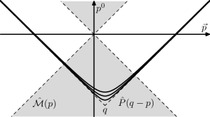
Figure 1.1. The convolution ${\hat{\mathcal{M}}}*\hat{P}$.

Therefore, the existence of the integral as well as its value might depend sensitively on an ultraviolet regularization. Since in this section we work with the unregularized fermionic projector, we simply impose that (1.6.20) should hold even after the ultraviolet regularization has been removed.

Def. 1.6.3.

The fermionic projector satisfies the assumption of a distributional $\mathcal{M}P$-product if for every $q$ for which $\hat{Q}(q)$ exists, the convolution integral (1.6.20) is well-defined without regularization and coincides with $\hat{Q}(q)$.

We point out that the above assumption is not merely a technical simplification, but it makes a highly non-trivial statement on the high-energy behavior of the physical fermionic projector. Ultimately, it needs to be justified by an analysis of the variational principle with ultraviolet regularization. At this stage, it can at least be understood from the fact that the assumption of a distributional $\mathcal{M}P$-product makes our stability analysis robust to regularization details. This means physically that the system should also be stable under “microscopic” perturbations of the fermionic projector on the Planck scale.

In what follows we will assume that the conditions in Def. 1.6.2 and Def. 1.6.3 are satisfied. Then the convolution integral (1.6.20) is well-defined for all $q\in\mathcal{C}^{\land}$. This implies that $\hat{\mathcal{M}}(p)$ must be a well-defined distribution on the set $\overline{\mathcal{C}^{\land}}\cup\{p\mid p^{2}<0\}$. Furthermore, since both $\hat{P}$ and $\hat{Q}$ are Lorentz invariant, we may assume that $\hat{\mathcal{M}}$ is also Lorentz invariant (otherwise we could replace $\hat{\mathcal{M}}$ by its Lorentz invariant part, and (1.6.20) would remain true). But if $\mathcal{M}(x,y)$ is Lorentz invariant, it involves no bilinear contribution, and its vector component is a multiple of $y-x$. According to (1.6.19), the matrix $\mathcal{M}(x,y)$ commutes with $A$. This implies that, for all $x,y$ for which $\mathcal{M}(x,y)\neq 0$, the matrix $A$ involves no bilinear contribution. Since the bilinear part of $A$ is given by the commutator of $P(x,y)$ and $P(y,x)$, we find that $P(x,y)$ and $P(y,x)$ commute. It follows that $A_{xy}=A_{yx}$ for all $x,y$ for which $\mathcal{M}(x,y)\neq 0$. As a consequence, $\mathcal{M}(x,y)=\mathcal{M}(y,x)$, and thus

$$\hat{\mathcal{M}}(-p)\;=\;\hat{\mathcal{M}}(p)\>.$$ (1.6.21)

This identity yields that $\hat{\mathcal{M}}$ is a well-defined distribution even on $\mathcal{C}^{\lor}$. We thus come to the following conclusion.

Proposition 1.6.4.

If the fermionic projector is state stable and the $\mathcal{M}P$-product is distributional, then $\hat{\mathcal{M}}(p)$ is a Lorentz invariant distribution of even parity (1.6.21).

This proposition poses a strong constraint for the ultraviolet regularization of the fermionic projector. It is a difficult question whether there are regularizations which satisfy this constraint. But at least we can say that the result of Proposition 1.6.4 does not immediately lead to inconsistencies, as the following lemma shows.

Lemma 1.6.5.

For all actions considered in §1.5, there is a distribution $\tilde{\mathcal{M}}$ on $M$ which coincides with $\mathcal{M}$ away from the light cone,

$$\tilde{\mathcal{M}}(y-x)\;=\;\mathcal{M}(x,y)\qquad\mbox{for all}\,\,x,y\in M\,\,\mbox{with}\,\,(y-x)^{2}\neq 0\,.$$

Proof. An explicit calculation using (1.6.19) and the representation of $P(x,y)$ with Bessel functions shows that for all actions considered in §1.5, $\mathcal{M}(x,y)$ is for $\xi\equiv y-x$ inside the upper light cone a smooth function with the following properties. It can be written as

$$\mathcal{M}(\xi)\;=\;i\mbox{$\partial$ $/$}_{\xi}f(\xi^{2})+g(\xi^{2})\;\;\;\;\;\;\;\;\;\;(\xi\in I^{\land})$$

with complex-valued functions $f,g\in C^{\infty}(\mathbb{R}^{+})$, which have at most polynomial growth as $\xi^{2}\to\infty$ and at most a polynomial singularity on the light cone, i.e.

$$|f(\xi^{2})|+|g(\xi^{2}|\;\leq\;c\left(\xi^{2n}+\frac{1}{\xi^{2n}}\right)$$

for suitable constants $c>0$, $n\in\mathbb{N}$.

Setting $z=\xi^{2}$, the Laplacian of a Lorentz invariant function $h(\xi^{2})$ is computed to be

$$\Box h(z)\;=\;4zh^{\prime\prime}(z)+8h^{\prime}(z)=\frac{4}{z}(z^{2}h^{\prime}(z))^{\prime}\,.$$ (1.6.22)

This allows us to invert the Laplacian explicitly,

$$\Box^{-1}h(z)\;=\;\frac{1}{4}\int^{z}_{z_{0}}\frac{d\tau}{\tau^{2}}\int^{\tau}_{\tau_{0}}\sigma\>h(\sigma)\>d\sigma$$ (1.6.23)

with two free constants $\tau_{0}$ and $z_{0}$. We choose $z_{0}=1$ and set $\tau_{0}=0$ if $\int^{1}_{0}\sigma|h(\sigma)|d\sigma<\infty$ and $\tau_{0}=1$ otherwise. Then applying $\Box^{-1}$ decreases the order of the pole on the light cone by one. Hence the functions

$$F^{\lor}(\xi)\;=\;\Box^{-n-1}f(\xi^{2})\>,\;\;\;\;\;\;\;\;\;\;G^{\lor}(\xi)\;=\;\Box^{-n-1}g(\xi^{2})$$

are smooth functions on $I^{\lor}$ which are locally bounded near the light cone and have at most polynomial growth as $\xi^{2}\to\infty$. Repeating the above construction inside the lower light cone gives rise to functions $F^{\land}$ and $G^{\land}$ on $I^{\land}$. Extending these functions by zero outside their respective domains of definition, the functions

$$F\;=\;F^{\lor}+F^{\land}\>,\;\;\;\;\;\;\;\;\;\;G\;=\;G^{\lor}+G^{\land}$$

are regular distributions on $M$. By construction, the distribution

$$\tilde{\mathcal{M}}\;=\;i\mbox{$\partial$ $/$}\Box^{n+1}F+\Box^{n+1}G$$

coincides inside the light cone with $\mathcal{M}$ and vanishes outside the light cone.    

The next lemma states a few important properties of the distribution $\hat{\mathcal{M}}$.

Lemma 1.6.6.

Under the assumptions of Proposition 1.6.4, the vector component of $\hat{\mathcal{M}}$ is supported inside the mass cone $\{p\mid p^{2}\geq 0\}$. If the scalar component of $\mathcal{M}$ has a nonvanishing contribution with the following asymptotics as $I\ni\xi\to 0$,

$$\mathcal{M}(\xi)\;\sim\;\xi^{2r}\log^{s}\xi^{2}\quad\mbox{with}\quad r,s\in\mathbb{Z},\,\,s\geq 1\,,$$ (1.6.24)

then its Fourier transform satisfies outside the mass cone for some $c>0$ the bound

$$|\hat{\mathcal{M}}(p)|\;\geq\;\frac{1}{c}(-p^{2})^{-2-r}\quad{\mbox{if~{}$p^{2}<-c$}}\,.$$ (1.6.25)

Proof. The statement for the vector component immediately follows from a symmetry argument: Due to Lorentz invariance, the vector component of $\hat{\mathcal{M}}(p)$ can be written as $p\mbox{ $/$}f(p)$ with a scalar distribution $f$. Since $\hat{\mathcal{M}}$ has even parity (1.6.21), it follows that $f(-p)=-f(p)$. Again using Lorentz invariance, we conclude that $f(p)$ vanishes if $p$ is outside the mass cone.

For the scalar component of $\hat{\mathcal{M}}$, the above symmetry argument does not apply, and (as can easily be verified by an explicit calculation) there is indeed a contribution outside the mass cone. More specifically, in the case $r\geq 0$ we can rescale the Fourier transform by $\xi\to\tau^{-1}\xi$,

$$\int\xi^{2r}\log^{s}(\xi^{2})\>e^{i\tau p\xi}\>d^{4}\xi\;=\;\tau^{-4-2r}\int\xi^{2r}(\log\xi^{2}-\log\tau^{2})^{s}\>e^{ip\xi}\>d^{4}\xi\,,$$

and obtain that (1.6.24) gives rise to a contribution to $\hat{\mathcal{M}}$ with the following asymptotics as $p^{2}\to-\infty$,

$$\hat{\mathcal{M}}(p)\;\sim\;(-p^{2})^{-2-r}\>(\log^{s}(-p^{2})+\mbox{l.o.t.})\;\;\;\;\;\;\;\;\;\;(r\geq 0)\,,$$ (1.6.26)

where ‘l.o.t.’ denotes lower order in $\log(-p^{2})$. If $r<0$, the singularity on the light cone cannot be treated with this scaling argument. But we can nevertheless compute the Fourier transform by iteratively applying the operator $\Box^{-1}_{p}$,

$$(-\Box_{p})^{2r}\int\log^{s}(\xi^{2})\>e^{ip\xi}d^{4}\xi\;=\;\int\xi^{2r}\log^{s}(\xi^{2})\>e^{ip\xi}d^{4}\xi\,.$$

Using (1.6.23) and (1.6.26), we obtain a contribution to $\hat{\mathcal{M}}(p)$ with the following asymptotics as $p^{2}\to-\infty$,

$$\hat{\mathcal{M}}(p)\;\sim\;(-p^{2})^{-2-r}\>(\log^{s+1}(\xi^{2})+\mbox{l.o.t.})\;\;\;\;\;\;\;\;\;\;(r<0)$$ (1.6.27)

(here we do not need to worry about the integration constants in (1.6.23) because these correspond to contributions localized on the light cone, which will be considered separately below, see (1.6.28)). The asymptotic formulas (1.6.26, 1.6.27) explain the estimate (1.6.25). However, the proof is not yet finished because the singular part of $\mathcal{M}$ which is localized on light cone might give rise to a contribution to $\hat{\mathcal{M}}$ which cancels (1.6.26) or (1.6.27). Thus it remains to show that all contributions to $\mathcal{M}$ which are localized on the light cone have an asymptotics different from (1.6.26, 1.6.27) and thus cannot compensate these contributions.

A scalar Lorentz invariant distribution $h$ which is localized on the light cone satisfies for some $n>0$ the relation $\xi^{2n}h(\xi)=0$. Hence its Fourier transform is a distributional solution of the equation

$$\Box^{n}\hat{h}(p)\;=\;0\,.$$

In the case $n=1$, we see from (1.6.22) that away from the mass cone, $\hat{h}(p)$ must be a linear combination of the functions $1$ and $p^{-2}$. By iteratively applying (1.6.23) one finds that for general $n$, $\hat{h}$ is of the form

$$\frac{1}{p^{2}}\,\,\mbox{(polynomial in $p^{2}$)}\,\,+\log(-p^{2})\,\,\mbox{(polynomial in $p^{2}$)}$$ (1.6.28)

The asymptotics of these terms as $p^{2}\to-\infty$ is clearly different from that in (1.6.26, 1.6.27).    

We are now ready to prove the main result of this section.

Theorem 1.6.7.

Consider the action corresponding to a Lagrangian of type (1.5.16). Assume that the fermionic projector of the vacuum is state stable and that the $\mathcal{M}P$-product is distributional (see Def. 1.6.2 and Def. 1.6.3). Then $n=1$.

Proof. Since here we consider only one sector, we need to change the normalization of the spectral weight in (1.5.16),

$$\mathcal{L}[A]=|A^{2n}|-\frac{1}{4}|A^{n}|^{2}\,.$$

According to Lemma 1.6.1, $\mathcal{L}$ vanishes identically for spacelike $y-x$, whereas for timelike $y-x$ we may replace the spectral weight by an ordinary trace. Hence away from the light cone and up to an irrelevant constant factor $2n$,

$$\mathcal{M}\;=\;\left[A^{n}-\frac{1}{4}\mbox{\rm{Tr}\/}(A^{n})\right]A^{n-1}\,.$$ (1.6.29)

According to Proposition 1.6.4, $\hat{\mathcal{M}}$ is a Lorentz invariant distribution of even parity. Following Def. 1.6.2 and Def. 1.6.3, the convolution integral (1.6.20) should be well-defined for any $q$ inside the lower mass cone. According to Lemma 1.6.6, the vector component of $\hat{\mathcal{M}}$ is supported inside the closed mass cone. Thus for the corresponding contribution to (1.6.20), the integration range is indeed compact (see Figure 1.1), and so (1.6.20) is well-defined in the distributional sense.

It remains to consider the scalar component of $\hat{\mathcal{M}}$. This requires a more detailed analysis. We again write the fermionic projector in the form (1.3.4, 1.6.6),

$$P(x,y)\;=\;i\xi\mbox{ $/$}f+h\,.$$

Using the representation (LABEL:l:3.1) of the distribution $T_{m^{2}}=\frac{1}{2}(P_{m^{2}}-K_{m^{2}})$ in position space, we can write $f$ and $g$ in the upper light cone as

$$f = \frac{c_{1}}{\xi^{4}}+\frac{c_{2}}{\xi^{2}}+\alpha\>(\log\xi^{2}+i\pi)+\beta$$

$$g = \frac{c_{3}}{\xi^{2}}+\gamma\>(\log\xi^{2}+i\pi)+\delta$$

with constants $c_{j}\neq 0$ and smooth real function $\alpha,\beta,\gamma,\delta$ with $\gamma_{0}:=\gamma(0)\neq 0$. A short calculation yields

$$A = \xi^{2}|f|^{2}+|h|^{2}-\xi\mbox{ $/$}\mbox{Im}(f\overline{h})$$

$$= \gamma^{2}_{0}\log^{2}\xi^{2}+\mbox{(lower orders in $\log\xi^{2}$)}\>+\>\xi\mbox{ $/$}\left(\frac{1}{\xi^{4}}+\mbox{(higher orders in $\xi^{2}$)}\right)\,.$$

The important point is that the vector component of $A$ involves no logarithms, whereas the scalar component involves terms $\sim\log^{2}\xi^{2}$. Substituting this expansion of $A$ into (1.6.29), we obtain for the scalar component of $\mathcal{M}$ sums of expressions of the general form $\xi^{2r}\log^{s}\xi^{2}$. We select those terms for which $s$ is maximal, and out of these terms for which $r$ is minimal. We get a contribution only when both the square bracket and the factor $A^{n-1}$ in (1.6.29) contain an odd number of Dirac matrices, and a short computation yields the asymptotics

$${\mathcal{M}}\;\sim\;(n-1)\>\xi^{-6}\log^{4n-6}\xi^{2}\,.$$ (1.6.30)

If $n=1$, the scalar component of $\hat{\mathcal{M}}$ vanishes, and we get no further conditions. However if $n>1$, Lemma 1.6.6 yields that $\hat{\mathcal{M}}(p)$ is outside the mass cone for large $p$ bounded away from zero by

$$|\hat{\mathcal{M}}(p)|\;\geq\;-\frac{p^{2}}{c}\,.$$

As a consequence, the convolution integral (1.6.20) diverges.    

We close this section with a few remarks. First, we can now discuss the stability of the vacuum for the polynomial actions (1.5.1). The strong analysis on the light cone in §1.5 forced us to only consider polynomial Lagrangians which vanish identically if $A$ has two independent eigenvalues. According to Lemma 1.6.1, this implies that $Q$ vanishes identically away from the light cone, and so the above stability analysis becomes trivial. Indeed, the following general consideration shows that for polynomial actions, the vacuum is not stable in the strict sense: Under the only assumption that $A$ has vector-scalar structure, the matrix $A$ has at most two independent eigenvalues (see (1.3.12) and Lemma 1.3.1), and so the Lagrangian vanishes identically. Thus the variational principle is trivial; it gives no conditions on the structure of the fermionic projector of the vacuum.

It might seem confusing that in the above analysis, the operator $Q(\xi)$ had poles on the light cone (see (1.6.30, 1.6.18)), although it vanishes identically in the formalism of the continuum limit. This can be understood from the fact that on the light cone, the matrix $A$ has a pair of complex conjugated eigenvalues (see (1.3.30)), whereas away from the light cone its eigenvalues are in general distinct real eigenvalues (see Lemma 1.6.1). If a matrix has non-real eigenvalues, this property remains valid if the matrix is slightly perturbed. Therefore, treating the eigenvalues of $A$ perturbatively, it is impossible to get from the region on the light cone to the region away from the light cone. This is the reason why the result of Lemma 1.6.1 cannot be obtained in the formalism of the continuum limit. The transition between the asymptotic regions near and away from the light cone can be studied only by analyzing the EL equations with regularization in detail, and this goes beyond the scope of this book. However, we point out that the order of the pole in (1.6.30) is lower than the order of all singularities which we will study in the continuum limit. This justifies that we can neglect (1.6.30) in what follows; taking into account (1.6.30) would have no effect on any of the results in this book.

The above argument shows that from all Lagrangians mentioned in §1.5, only for (1.5.14) the vacuum can be stable (in the sense made precise in Theorem 1.6.7). The important question arises whether the above necessary conditions are also sufficient, i.e. if for the Lagrangian (1.5.14) the vacuum is indeed state stable. This question cannot be answered here; in any case a more detailed analysis would yield additional constraints for the mass parameters $m_{\alpha}$ and the regularization. But at least we can say that for the Lagrangian (1.5.14), the vacuum has very nice properties which point towards stability: First of all, $Q$ vanishes in the continuum limit. But it does not vanish identically away from the light cone, and thus the EL equations are non-trivial in the vacuum. Furthermore, $Q(\xi)$ is supported in the light cone, giving an interesting (although not yet fully understood) link to causality. The crucial point for Theorem 1.6.7 is that the scalar component of $\mathcal{M}$ vanishes (as is obvious from (1.6.29)), and therefore $\hat{\mathcal{M}}$ is supported inside the mass cone (see Lemma 1.6.6). The last property implies via a simple support argument that, for $q$ inside the lower mass cone, the convolution integral (1.6.20) is finite (see Figure 1.1). This means that the stability conditions (ii) and (iii) of Def. 1.6.2 (which we did not consider here) could be analyzed without any assumption on the regularization. However, for $q$ outside the lower mass cone, the convolution integral (1.6.20) will in general diverge (see again Figure 1.1), indicating that the vacuum could be stable even under perturbations where fermionic states with momenta outside the lower mass cone are occupied.

Chapter 2 The Dynamical Gauge Group

We now begin the analysis of the continuum limit of the EL equations with interaction. In order to work in a concrete example, we shall analyze our model variational principle of §LABEL:psec15. But the methods as well as many of the results carry over to other variational principles, as will be discussed in the Remarks at the end of Chapter 2 and at the end of Chapter 3. We again consider the fermionic projector of the standard model §1.1. For the bosonic potentials in the corresponding auxiliary Dirac equation (LABEL:b) we make the ansatz

$${\mathcal{B}}\;=\;C\!\mbox{ $/$}+\gamma^{5}\>E\!\mbox{ $/$}+\Phi+i\gamma^{5}\>\Xi$$ (2.0.1)

with a vector potential $C$, an axial potential $E$ and scalar/pseudoscalar potentials $\phi$ and $\Xi$, which again in component notation ${\mathcal{B}}={\mathcal{B}}^{(a\alpha)}_{(b\beta)}$ we assume to be of the form

$$C\;=\;C^{a}_{b}\>\delta^{\alpha}_{\beta}\>,\;\;\;\;\;\;E\;=\;E^{a}_{b}\>\delta^{\alpha}_{\beta}\>,\;\;\;\;\;\;\phi\;=\;\phi^{(a\alpha)}_{(b\beta)}\>,\;\;\;\;\;\;\Xi\;=\;\Xi^{(a\alpha)}_{(b\beta)}\>.$$ (2.0.2)

Exactly as in §LABEL:jsec5 it is convenient to introduce the chiral potentials

$$A_{L\!/\!R}\;=\;C\pm E\>,$$ (2.0.3)

and to define the dynamical mass matrices by

$$mY_{L\!/\!R}\;=\;mY-\phi\mp i\Xi\>.$$ (2.0.4)

Then the auxiliary Dirac equation takes the form

$$\left(i\mbox{$\partial$ $/$}+\chi_{L}(\mbox{ $\!\!A$ $/$}_{R}-mY_{R})+\chi_{R}(\mbox{ $\!\!A$ $/$}_{L}-mY_{L})\right)P(x,y)\;=\;0\>.$$ (2.0.5)

Clearly, the potentials in (2.0.1) must be causality compatible (LABEL:89). We assume in what follows that this condition is satisfied, and we will specify what it means in the course of our analysis.

Let us briefly discuss the ansatz (2.0.1). The vector and axial potentials in (2.0.1) have a similar form as the gauge potentials in the standard model. Indeed, when combined with the chiral potentials (2.0.3), they can be regarded as the gauge potentials corresponding to the gauge group $U(8)_{L}\times U(8)_{R}$. This so-called chiral gauge group includes the gauge group of the standard model. At every space-time point, it has a natural representation as a pair of $8\times 8$ matrices acting on the sectors; we will work in this representation throughout. Compared to the most general ansatz for the chiral potentials, the only restriction in (2.0.3, 2.0.2) is that the chiral potentials are the same for the three generations. This can be justified from the behavior of the fermionic projector under generalized gauge transformations, as will be explained in Remark 2.2.3 below. The scalar potentials in (2.0.1) do not appear in the standard model, but as we shall see, they will play an important role in our description of the interaction (here and in what follows, we omit the word “pseudo” and by a “scalar potential” mean a scalar or a pseudoscalar potential). We point out that we do not consider a gravitational field. The reason is that here we want to restrict attention to the interactions of the standard model. But since the principle of the fermionic projector respects the equivalence principle, one could clearly include a gravitational field; we plan to do so in the future. Compared to a general multiplication operator, (2.0.1) does not contain bilinear potentials (i.e. potentials of the form $H_{jk}\sigma^{jk}$ with $\sigma^{jk}=\frac{i}{2}[\gamma^{j},\gamma^{k}]$). Clearly, bilinear potentials do not appear in the standard model, but it is not obvious why they should be irrelevant in our description. Nevertheless, we omit bilinear potentials in order to keep the analysis as simple as possible. To summarize, (2.0.1) is certainly not the most general ansatz which is worth studying. But since the potentials in (2.0.1) are considerably more general than the gauge potentials in the standard model, it seems reasonable to take (2.0.1) as the starting point for our analysis.

2.1. The Euler-Lagrange Equations to Highest Degree on the Light Cone

We come to the detailed calculations. We again work with the spectral decomposition of $A_{xy}$ and proceed degree by degree on the light cone. In this section we consider the highest degree. Then the fermionic projector is influenced only by the chiral potentials (and not by the scalar potentials or the particle states), and the chiral potentials merely describe local phase transformations of the fermionic projector. More precisely, truncating all contributions of degree $<2$ and denoting this “truncated fermionic projector” by $P_{0}(x,y)$, we have (see §LABEL:jsec5 and Appendix LABEL:pappLC)

$$P_{0}(x,y)\;=\;\left(\chi_{L}\>X_{L}\>{\mbox{ \footnotesize{L}}}\displaystyle\int_{x}^{y}+\chi_{R}\>X_{R}{\mbox{ \footnotesize{R}}}\displaystyle\int_{x}^{y}\right)\frac{i}{2}\>\xi\mbox{ $/$}\>T^{(-1)}_{[0]}(x,y)\>,$$ (2.1.1)

where we used for the ordered exponentials the short notation

$${\mbox{ \footnotesize{c}}}\displaystyle\int_{x}^{y}\;=\;{\mbox{Pexp}}\left(-i\int_{0}^{1}A_{c}^{j}(\tau y+(1-\tau)x)\>(y-x)_{j}\>d\tau\right)$$ (2.1.2)

with $c=L$ or $R$. We also truncate the matrix $A_{xy}$ by setting

$$A_{0}(x,y)\;=\;P_{0}(x,y)\>P_{0}(y,x)\>.$$

It follows from (2.1.1) that

$$A_{0}\;=\;\left\{\chi_{L}\>X_{L}\>{\mbox{ \footnotesize{L}}}\displaystyle\int_{x}^{y}{\mbox{ \footnotesize{R}}}\displaystyle\int_{y}^{x}X_{R}\>+\>\chi_{R}\>X_{R}\>{\mbox{ \footnotesize{R}}}\displaystyle\int_{x}^{y}{\mbox{ \footnotesize{L}}}\displaystyle\int_{y}^{x}X_{L}\right\}\>\frac{1}{4}\>(\xi\mbox{ $/$}\>T^{(-1)}_{[0]})(\overline{\xi\mbox{ $/$}\>T^{(-1)}_{[0]}})\>.$$ (2.1.3)

We can assume that the matrix inside the curly brackets is diagonalizable; indeed, this is the generic situation, and the general case immediately follows from it by approximation. The matrix $A_{0}$ is invariant on the left- and right-handed spinors. If considered on one of these invariant subspaces, the curly brackets depend only on the sector indices $a,b=1,\ldots,8$, whereas the factors to their right involve only Dirac matrices. This allows us to factor the spectral decomposition of $A_{0}$ as follows. We first diagonalize the phase factor, i.e.

$$W_{c}\;\equiv\;X_{c}\;{\mbox{ \footnotesize{c}}}\displaystyle\int_{x}^{y}{\mbox{ \footnotesize{$\overline{c}$}}}\displaystyle\int_{y}^{x}\!X_{\overline{c}}\;=\;\sum_{n=1}^{8}\nu_{nc}\>I_{nc}$$ (2.1.4)

with eigenvalues $\nu_{nc}$ (counting multiplicities) and corresponding spectral projectors $I_{nc}$, where $\overline{c}$ is defined by $\overline{L}=R$ and $\overline{R}=L$. The matrices $W_{L}$ and $W_{R}$ are obtained from each other by taking their adjoint. Thus we can arrange that the same holds for their spectral decompositions,

$$\overline{\nu_{nc}}\;=\;\nu_{n\overline{c}}\>,\;\;\;\;\;\;\;\;\;\;I_{nc}^{*}\;=\;I_{n\overline{c}}\>.$$ (2.1.5)

The spectral representation of the second term in (2.1.3) is computed exactly as described in §1.3. More precisely, it is obtained from (1.3.8, 1.3.10) by setting $h$ to zero, i.e. similar to (1.3.22, 1.3.23),

$$\frac{1}{4}\>(\xi\mbox{ $/$}\>T^{(-1)}_{[0]})(\overline{\xi\mbox{ $/$}\>T^{(-1)}_{[0]}})\;=\;\sum_{s=\pm}\lambda_{s}\>F_{s}$$ (2.1.6)

with

$$\lambda_{s} = \frac{1}{4}\>T^{(-1)}_{[0]}\>\overline{T^{(-1)}_{[0]}}\>\times\>\left\{\begin{array}[]{cl}z&{\mbox{if $s=+$}}\\ \overline{z}&{\mbox{if $s=-$}}\end{array}\right.$$ (2.1.9)

$$F_{s} = \frac{1}{z-\overline{z}}\>\times\>\left\{\begin{array}[]{cl}\xi\mbox{ $/$}\overline{\xi\mbox{ $/$}}-\overline{z}&{\mbox{if $s=+$}}\\ -\xi\mbox{ $/$}\overline{\xi\mbox{ $/$}}+z&{\mbox{if $s=-$ .}}\end{array}\right.$$ (2.1.12)

Combining (2.1.4) and (2.1.6) gives

$$A_{0}\;=\;\sum_{n=1}^{8}\>\sum_{c=L,R}\>\sum_{s=\pm}\lambda_{ncs}\>F_{ncs}$$ (2.1.13)

with

$$\lambda_{ncs}\;=\;\nu_{nc}\>\lambda_{s}\>,\;\;\;\;\;\;\;\;\;\;F_{ncs}\;=\;\chi_{c}\>I_{nc}\>F_{s}\>.$$ (2.1.14)

It might be surprising at first sight that, although $A_{0}$ clearly is a gauge-invariant expression, the phase shifts described by the ordered exponentials in (2.1.1) do not drop out in (2.1.3). Let us explain in detail how this comes about. We first recall that under gauge transformations, the truncated fermionic projector transforms like

$$P_{0}(x,y)\;\longrightarrow\;U(x)\>P_{0}(x,y)\>U(y)^{-1}\>,$$ (2.1.15)

where $U$ is unitary with respect to the spin scalar product, $U(x)^{*}=U(x)^{-1}$. These $U(2N,2N)$ gauge transformations correspond to a local symmetry of the system, which is related to the freedom in choosing a local basis for the spinors (see §LABEL:psec11). When forming the closed chain, the gauge transformations at $y$ drop out,

$$P_{0}(x,y)\>P_{0}(y,x)\;\longrightarrow\;U(x)\>P_{0}(x,y)\>P_{0}(y,x)\>U(x)^{-1}\>.$$

In order to see the relation between the phase transformations in (2.1.1) and the above gauge transformations, it is useful to consider the situation when the chiral potentials have the form of pure gauge potentials, i.e.

$$A_{c}^{j}\;=\;iV_{c}\>(\partial^{j}V_{c}^{-1})$$ (2.1.16)

with unitary operators $V_{L},V_{R}\in U(8)$. Then the ordered exponential (2.1.2) reduces to a product of unitary transformations at the two end points,

$${\mbox{ \footnotesize{c}}}\displaystyle\int_{x}^{y}\;=\;V_{c}(x)\>V_{c}(y)^{-1}\>.$$

Using that the potentials are causality compatible, (2.1.1) becomes

$$P_{0}(x,y)\;=\;\sum_{c=L,R}\chi_{c}\>V_{c}(x)\>X_{c}\left(\frac{i}{2}\>\xi\mbox{ $/$}\>T^{(-1)}_{[0]}(x,y)\right)V_{c}(y)^{-1}\>.$$ (2.1.17)

Hence the left- and right-handed components of $P_{0}$ are transformed independently by $V_{L}$ and $V_{R}$, respectively. In order to write these transformations in a form similar to (2.1.15), we combine $V_{L}$ and $V_{R}$ into one operator $V$,

$$V\;=\;\chi_{L}\>V_{L}+\chi_{R}\>V_{R}\>.$$

The effect of the chiral potentials in (2.1.17) is then described by the transformation

$$P_{0}(x,y)\;\longrightarrow\;V(x)\>P_{0}(x,y)\>V(y)^{*}\>,$$

and thus the closed chain transforms according to

$$P_{0}(x,y)\>P_{0}(y,x)\;\longrightarrow\;V(x)\>P_{0}(x,y)\>V(y)^{*}\>V(y)\>P_{0}(y,x)\>V(x)^{*}\>.$$ (2.1.18)

The point is that the transformation $V$ is in general not unitary, because

$$V^{*}\;=\;\chi_{R}\>V_{L}^{-1}+\chi_{L}V_{R}^{-1}\;\stackrel{{\scriptstyle\mbox{\tiny{in general}}}}{{\neq}}\;\chi_{L}\>V_{L}^{-1}+\chi_{R}V_{R}^{-1}\;=\;V^{-1}\>.$$

More precisely, $V$ is unitary if and only if $V_{L}=V_{R}$ at every space-time point. According to (2.1.16), this implies the condition $A_{L}\equiv A_{R}$. From (2.0.3) we conclude that $V$ is unitary if and only if the axial potentials $E$ in (2.0.1) are identically equal to zero. This means that only the subgroup $U(8)\subset U(8)_{L}\times U(R)_{R}$ of the chiral gauge group, which gives rise to the vector potential $C$ in (2.0.1), describes local unitary transformations of the fermionic projector and thus corresponds to a local gauge symmetry in the sense of §LABEL:psec11. We refer to this subgroup of the chiral gauge group as the free gauge group ${\mathcal{F}}$; it can be identified with a subgroup of the gauge group, ${\mathcal{F}}\subset U(2N,2N)$ (we remark for clarity that the other degrees of freedom of the gauge group $U(2N,2N)$ are related to the gravitational field §LABEL:isec5 and are thus not considered here). The axial potentials, however, describe local transformations which are not unitary and thus cannot be identified with gauge transformations in the sense of §LABEL:psec11. These non-unitary transformations do not correspond to an underlying local symmetry of the system. The interpretation of these results is that the chiral gauge group is spontaneously broken, and only its subgroup ${\mathcal{F}}$ corresponds to an unbroken local symmetry of the system.

A simple way to understand why the chiral gauge group is spontaneously broken is that axial potentials describe relative phase shifts between the left- and right-handed components of the fermionic projector. Such relative phases do not drop out when we form composite expressions, as one sees in (2.1.18) or, more generally, in (2.1.3). By imposing that the relative phases be zero in all composite expressions, we can distinguish those systems in which the axial potentials vanish identically. In this way, one can fix the gauge up to global chiral gauge transformations (i.e. transformations of the form (2.1.17) with constant matrices $V_{c}$) and up to local free gauge transformations. Since this gauge fixing argument makes use of the phases which appear in $P_{0}(x,y)$, one may regard the chiral gauge symmetry as being spontaneously broken by the fermionic projector.

The spontaneous breaking of the chiral gauge symmetry by the fermionic projector has, at least on the qualitative level, some similarity to the Higgs mechanism in the standard model. We recall that in the Higgs mechanism one arranges by a suitable quartic potential in the classical Lagrangian that the Higgs field $\Phi$ has a non-trivial ground state, i.e. $\Phi\neq 0$ in the vacuum. The Higgs field is acted upon by a local gauge group. Since $\Phi\neq 0$, one can, by prescribing the phase of $\Phi$, fix the gauge globally. This shows that the local gauge symmetry is spontaneously broken by the Higgs field, a fact which can then be used to give the gauge bosons mass. In our setting, we also have in the vacuum a non-trivial object, namely the fermionic projector, which is composed of the Dirac seas corresponding to the leptons and quarks. Thus our situation is indeed quite similar to the Higgs mechanism, if one only keeps in mind that the role of the Higgs field in our description is played by the fermionic projector of the vacuum. Clearly, this analogy does not carry over to the mathematical details. But also in our description, the spontaneous symmetry breaking makes it possible that undifferentiated gauge potentials enter the EL-equations, giving the hope that the corresponding gauge bosons might be massive.

Since the chiral gauge symmetry is spontaneously broken, we cannot expect that the EL equations admit chiral potentials corresponding to the whole group $U(8)_{L}\times U(8)_{R}$. In order to quantify which restrictions for the chiral potentials we get, we must work in a more general setting and introduce a suitable mathematical notation. Contributions to the fermionic projector which involve the phases of the chiral potentials, but not the gauge fields, currents, or scalar potentials, are called gauge terms. Likewise, we refer to the contributions of the gauge terms to a composite expression in the fermionic projector as the gauge terms in the respective expression. The simplest examples for gauge terms are (2.1.1) or (2.1.3), but we shall encounter gauge terms to lower degree on the light cone as well.

Def. 2.1.1.

A subgroup ${\mathcal{G}}$ of the chiral gauge group is called a dynamical gauge group if the gauge terms of the potentials corresponding to ${\mathcal{G}}$ vanish in the EL equations. The subgroup ${\mathcal{G}}\cap{\mathcal{F}}$ is the free dynamical gauge group.

Clearly, this definition does not give a unique dynamical gauge group. In particular, every subgroup of a dynamical gauge group is again a dynamical gauge group. Since we want to choose the dynamical gauge group as large as possible, we will always restrict attention to dynamical gauge groups which are maximal in the sense that they are not contained in a larger dynamical gauge group.

We first analyze the gauge term (2.1.1) in the EL equations corresponding to our variational principle (1.5.14). We only consider the highest degree on the light cone, which is degree 5. This gives the following result.

Theorem 2.1.2.

The eigenvalues $\nu_{nc}$ of $W_{c}$ must satisfy the conditions

$$\nu_{8c}=0\quad{\mbox{and}}\quad|\nu_{nc}|=|\nu_{n^{\prime}c^{\prime}}|{\mbox{ for $n,n^{\prime}=1,\ldots,7$ and $c,c^{\prime}=L,R$}}.$$ (2.1.19)

The dynamical gauge group ${\mathcal{G}}$ is restricted by

$${\mathcal{G}}\subset(U(7)\times U(1))_{L}\times(U(7)\times U(1))_{R}\>,$$ (2.1.20)

where the $U(7)$ are unitary matrices acting on the seven massive sectors, and the $U(1)$ act on the neutrino sector.

If conversely the conditions (2.1.19) or (2.1.20) are satisfied, then the EL equations are satisfied to degree $5$ on the light cone.

It is easy to see that the conditions in the above theorem are sufficient for the EL equations to be satisfied, and this consideration also gives an idea of how these conditions come about. Namely, suppose that (2.1.20) holds. Then the dynamical gauge potentials are invariant on the massive sectors as well as on the neutrino sector. Using a block matrix notation where the first component refers to the massive sectors and the second component to the neutrino sector, we see from (2.1.4) that the matrices $W_{L}$ and $W_{R}$ have the form

$$W_{L}\;=\;\left(\begin{array}[]{cc}U&0\\ 0&0\end{array}\right),\;\;\;\;\;\;\;\;\;\;W_{R}\;=\;\left(\begin{array}[]{cc}U^{*}&0\\ 0&0\end{array}\right)$$ (2.1.21)

with $U$ a unitary $7\times 7$ matrix. Hence their eigenvalues $\nu_{nc}$ satisfy the conditions (2.1.19). Using (1.4.7), the gradient of the Lagrangian is computed to be

$${\mathcal{M}}[A]\;=\;2\sum_{k=1}^{K}\left\{\left(|\lambda_{k}|-\frac{1}{28}\>|A|\right)\frac{\overline{\lambda_{k}}}{|\lambda_{k}|}\right\}F_{k}\>.$$ (2.1.22)

We saw in §1.5 that the curly brackets vanish in the vacuum. If (2.1.19) is satisfied, the gauge terms change the eigenvalues $\lambda_{ncs}$ only by a phase (2.1.14). Since these phases drop out when absolute values are taken, the curly brackets in (2.1.22) are zero even with interaction (to the highest degree on the light cone). According to (1.2.7), this implies that $Q$ vanishes, and so the EL equations are satisfied.

It is more difficult to show that the conditions (2.1.19) and (2.1.20) are also necessary. We give the proof in detail.
Proof of Theorem 2.1.2. Using the argument given after the statement of the theorem, it remains to show that the conditions (2.1.19) and (2.1.20) are necessary. Substituting the spectral decomposition of $A_{0}$ into (1.5.4), we obtain, in analogy to (1.4.8), the following representation for $Q$,

$$Q(x,y)\;=\;\frac{1}{2}\>\sum_{n,c,s}\frac{\partial{\mathcal{L}}(\lambda^{xy})}{\partial\lambda^{xy}_{ncs}}\>F^{xy}_{ncs}\>P_{0}(x,y)\>+\>(\deg<5).$$

Computing the Euler-Lagrange equations similar to (1.4.10) and keeping track of the chiral cancellations, we obtain in analogy to (1.4.12) the equation

$$\sum_{n,c,s}\frac{\partial{\mathcal{L}}(\lambda^{xy})}{\partial\lambda^{xy}_{ncs}}\>F^{xy}_{ncs}\>P_{0}(x,y)\>{\mbox{ \footnotesize{$\overline{c}$}}}\displaystyle\int_{y}^{z}X_{\overline{c}}\>+\>(\deg<5)\;=\;0\>,$$

and by multiplying from the right by the macroscopic unitary matrix ${\mbox{ \footnotesize{$\overline{c}$}}}\displaystyle\int_{z}^{y}\!$, we can arrange that $z=y$. We substitute (2.1.1) as well as the right of (2.1.14) and apply (1.3.25) to obtain

$$\sum_{nc}\frac{\partial{\mathcal{L}}(\lambda)}{\partial\lambda_{nc-}}\>\chi_{c}\>I_{nc}\left\{X_{c}\>{\mbox{ \footnotesize{c}}}\displaystyle\int_{x}^{y}{\mbox{ \footnotesize{$\overline{c}$}}}\displaystyle\int_{y}^{x}X_{\overline{c}}\right\}\left(\frac{i}{2}\>\xi\mbox{ $/$}\>T^{(-1)}_{[0]}\right)\>+\>(\deg<5)\;=\;0\>.$$

The curly brackets coincide with the matrix $W_{c}$, and since $I_{nc}$ is a spectral projector of this matrix, we simply get a scalar factor $\nu_{nc}$. Furthermore, we use the particular form of our Lagrangian (1.5.14) as well as the first equation in (2.1.14). This gives

$$i\sum_{n,c}\left(|\nu_{nc}|-\frac{1}{14}\>\sum_{n^{\prime},c^{\prime}}|\nu_{n^{\prime}c^{\prime}}|\right)\>\chi_{c}\>\xi\mbox{ $/$}\>I_{nc}\>\overline{\lambda_{-}}\>T^{(-1)}_{[0]}\;=\;0\>.$$ (2.1.23)

Using (1.3.22), the non-smooth factors are a monomial of degree five,

$$\overline{\lambda_{-}}\>T^{(-1)}_{[0]}\;=\;T^{(0)}_{[0]}\>T^{(-1)}_{[0]}\>\overline{T^{(-1)}_{[0]}}\>.$$ (2.1.24)

We cannot assume that this monomial is equal to zero. Namely, the fermionic projector differs to highest degree on the light cone from the fermionic projector of the vacuum only by macroscopic phase factors (this is guaranteed by the gauge invariance of the regularized causal perturbation expansion, see Appendix LABEL:pappB). Therefore, exactly as explained for the vacuum in §1.4, we can evaluate (2.1.23) even strongly. In particular, we can consider the regularization expansion of (2.1.23) (see §LABEL:psec24, §LABEL:psec25). This means that, in order to set the monomial (2.1.24) in (2.1.23) equal to zero, we would have to impose an infinite number of regularization conditions. We conclude that in order to satisfy (2.1.23), we must assume that the macroscopic prefactor vanishes. Using that the spectral projectors $I_{nc}$ are linearly independent, we get the conditions

$$\left(|\nu_{nc}|-\frac{1}{14}\>\sum_{n^{\prime},c^{\prime}}|\nu_{n^{\prime}c^{\prime}}|\right)|\nu_{nc}|^{2}\;=\;0\;\;\;\;\;\;\;\;\;\;{\mbox{for all $n,c$}}.$$

This implies that the absolute values of $14$ of the eigenvalues $\nu_{nc}$ must coincide, and that the remaining two eigenvalues must be zero. The matrix $W_{L}$ contains a factor $X_{R}$ and is thus singular of rank one. Choosing the numbering such that $\nu_{L8}=0$, it follows from (2.1.5) that also $\nu_{R8}=0$. Hence the two zero eigenvalues are those for $n=8$. This shows that (2.1.19) is a necessary condition.

Next we will show that (2.1.19) implies the constraint for the dynamical gauge group (2.1.20). We introduce for fixed $x$ and $y$ the abbreviations

$$U\;=\;{\mbox{ \footnotesize{L}}}\displaystyle\int_{x}^{y}{\mbox{ \footnotesize{R}}}\displaystyle\int_{y}^{x}\;\;\;\;\;\;\;\;\;\;{\mbox{and}}\;\;\;\;\;\;\;\;\;\;T\;=\;X_{R}\>.$$ (2.1.25)

We consider $U=(U^{a}_{b})$ and $T=(T^{a}_{b})$ as matrices on ${\mbox{\Bb C}}^{8}$ endowed with the standard Euclidean scalar product $\langle.,.\rangle$. Then $U$ is unitary, and $T$ is a projector of rank $7$. According to (2.1.5), the conditions (2.1.19) tell us that the matrix $UT$ must have $7$ eigenvalues on the unit circle and one zero eigenvalue. For a vector $u$ in the kernel of $UT$,

$$0\;=\;\langle UTu,\>UTu\rangle\;=\;\langle Tu,\>Tu\rangle\>,$$

where we used in the last step that $U$ is unitary. Thus $u$ is also in the kernel of $T$. On the other hand, if $u$ is an eigenvector of $UT$ corresponding to an eigenvalue on the unit circle,

$$|u|^{2}\;=\;\langle UTu,\>UTu\rangle\;=\;\langle Tu,\>Tu\rangle\>.$$

Since for a projector, $|Tu|<|u|$ unless $u$ is in the image of $T$, it follows that $u$ is also an eigenvector of $T$, of eigenvalue one. We conclude that every eigenvalue of $UT$ is also an eigenvalue of $T$, or equivalently that

$$[UT,\>T]\;=\;0\>.$$ (2.1.26)

Let us analyze what this commutator condition means for the chiral potentials. We already know from the causality compatibility condition that

$$[A_{R},T]\;=\;0\>.$$ (2.1.27)

Hence substituting the definition of $U$, (2.1.25), into (2.1.26) and using that the resulting condition must hold for all $x$ and $y$, we obtain that $[A_{L}T,T]=0$. Subtracting the adjoint and using that $T$ is idempotent gives the stronger statement

$$[A_{L},T]\;=\;0\>.$$ (2.1.28)

From (2.1.27) and (2.1.28) we conclude that the chiral potentials must be block diagonal in the sense that $(A_{c})^{a}_{b}=0$ if $a=8$ and $b\neq 8$ or vice versa. Such chiral potentials correspond precisely to the gauge group in (2.1.20).    

Remark 2.1.3.

We point out that the subgroup $U(1)_{L}\times U(1)_{R}$ of the gauge group in (2.1.20), which acts on the neutrino sector, is not uniquely determined and could be replaced by any other subgroup which contains $U(1)_{L}$. This can immediately be understood from the fact that the neutrino sector contains only left-handed particles, and thus the form of the potential $A_{R}$, which acts on the right-handed component, has no significance. To make this argument rigorous, we consider the Dirac equation (2.0.5). Since $P=XP$, we may replace the chiral potentials $A_{c}$ in (2.0.5) by $A_{c}X_{c}$, and this indeed makes the component of $A_{R}$ in the neutrino sector equal to zero, showing that this component is of no relevance. We conclude that we may arbitrarily change the subgroup $U(1)_{R}$ in (2.1.20); e.g. we could replace (2.1.20) by

$$(U(7)\times U(1))_{L}\times U(7)_{R}\;\;\;\;\;\;\;\;\;\;{\mbox{or}}\;\;\;\;\;\;\;\;\;\;(U(7)_{L}\times U(7)_{R})\times U(1)\>.$$ (2.1.29)

We do not write out this obvious arbitrariness in what follows; instead we will simply give the gauge groups in the most convenient form.

2.2. The Gauge Terms in the Euler-Lagrange Equations

We come to the analysis of the EL equations to the next lower degree $4$ on the light cone. According to the formulas of the light-cone expansion in Appendix LABEL:pappLC, the structure of the fermionic projector to the next lower degree is considerably more complicated than (2.1.1), because in addition to gauge terms, there are also contributions involving the chiral fields and currents as well as the scalar potentials. Fortunately, the following general argument allows us to distinguish these different types of contributions in the EL equations. In the formulas for $P(x,y)$, the gauge terms always involve ordered exponentials of the chiral potentials, integrated along the line segment $\overline{xy}=\{\alpha x+(1-\alpha)y,\>0\leq\alpha\leq 1\}$. We refer to such contributions as line contributions. The fields, currents and scalar potentials, however, are in the light-cone expansion evaluated at individual points, namely either at the end points $x,y$ or at an intermediate point $z\in\overline{xy}$; we call the corresponding contributions to the light-cone expansion point contributions. In the case of an evaluation at an intermediate point $z$, the point contribution clearly involves an integral over $z$ along $\overline{xy}$. But in contrast to the line contribution, where the chiral potentials at different points enter the ordered exponential in a nonlinear way, the line integrals in a point contribution simply takes averages of the potentials, fields, or currents along the line segment. For example by expanding the ordered exponential in a Dyson series (see Def. LABEL:2.5.4) and considering the higher order terms, one sees immediately that the line and point contributions are independent in the EL equations in the sense that the EL equations must be satisfied separately by the line and point contributions. Moreover, we can distinguish point contributions in the EL equations, provided that their configuration of the tensor indices is different. Therefore, the point contributions involving the scalar potentials, the chiral fields and the currents are independent in the EL equations as well.

Using the above arguments, we can study the gauge terms and the contributions involving the scalar potentials, the gauge fields and the currents separately. In the remainder of this section, we consider only the gauge terms. Thus we restrict attention to chiral potentials, i.e. instead of (2.0.5) we consider the Dirac equation

$$(i\mbox{$\partial$ $/$}-mY+\chi_{L}\>\mbox{ $\!\!A$ $/$}_{R}+\chi_{R}\>\mbox{ $\!\!A$ $/$}_{L})\>P(x,y)\;=\;0$$

with $Y$ a fixed matrix. We will return to the general Dirac equation (2.0.5) in Chapter 3.

Def. 2.2.1.

We introduce for $p\in\{4,\ldots,7\}$ the groups $B_{p},F_{p}\subset U(8)$ by

$$B_{p} = \{\>\underbrace{g\oplus\cdots\oplus g}_{p{\mbox{\scriptsize{ summands}}}}\oplus\underbrace{g^{-1}\oplus\cdots\oplus g^{-1}}_{7-p{\mbox{\scriptsize{ summands}}}}{\mbox{ with $g\in U(1)$}}\}$$ (2.2.1)

$$F_{p} = U(p)\times U(7-p)\times U(1)$$ (2.2.2)

and define corresponding subgroups ${\mathcal{B}}_{p}$ and ${\mathcal{F}}_{p}$ of the dynamical gauge group by

$${\mathcal{B}}_{p}\;=\;B_{p}\times\mbox{\rm 1 1}\;\subset\;U(8)_{L}\times U(8)_{R}\>,\;\;\;\;\;\;\;\;\;\;{\mathcal{F}}_{p}\;=\;\{{\mbox{$(g,g)$ with $g\in F_{p}$}}\}\;\subset\;{\mathcal{F}}\>.$$ (2.2.3)

Their product

$${\mathcal{G}}_{p}\;=\;{\mathcal{B}}_{p}\cdot{\mathcal{F}}_{p}\;\equiv\;\{{\mbox{$bf$ with $b\in{\mathcal{B}}_{p}$, $f\in{\mathcal{F}}_{p}$}}\}\;\subset\;U(8)_{L}\times U(8)_{R}$$ (2.2.4)

is called the ${\mbox{\em{p}}}^{\mbox{\scriptsize{th}}}$ dynamical gauge group.

In block matrix notation, the elements of $B_{p}$ and $F_{p}$ can be written as

$$\left(\begin{array}[]{ccc}z\>\mbox{\rm 1 1}_{p}&0&0\\ 0&z^{-1}\>\mbox{\rm 1 1}_{q}&0\\ 0&0&0\end{array}\right)\;\;\;\;\;\;\;\;\;\;{\mbox{and}}\;\;\;\;\;\;\;\;\;\;\left(\begin{array}[]{ccc}g&0&0\\ 0&h&0\\ 0&0&l\end{array}\right)\>,$$ (2.2.5)

respectively, where the first component refers to the first $p$ sectors, the second component to the next $q\equiv 7-p$ sectors and the last component to the neutrino sector. Here $z,l\in U(1)$, $g\in U(p)$ and $h\in U(q)$. Clearly, $B_{p}$ and ${\mathcal{B}}_{p}$ are group isomorphic to $U(1)$. Notice that ${\mathcal{B}}_{p}$ acts only the left-handed component. The group ${\mathcal{F}}_{p}$ transforms the left- and right-handed components in the same way, and so its corresponding gauge potentials are vector potentials. The groups ${\mathcal{B}}_{p}$ and ${\mathcal{F}}_{p}$ commute, and this ensures that their product (2.2.4) is again a group. It is easy to verify that ${\mathcal{F}}_{p}$ is indeed the largest subgroup of ${\mathcal{F}}$ which commutes with ${\mathcal{B}}_{p}$,

$${\mathcal{F}}_{p}\;=\;\left\{f\in{\mathcal{F}}\;|\;bfb^{-1}=f{\mbox{ for all }}b\in{\mathcal{B}}_{p}\right\}\>.$$

We introduce an abbreviation for the linear combination of monomials,

$$M\;\equiv\;T^{(0)}_{[1]}\>T^{(0)}_{[1]}\>\overline{T^{(-1)}_{[0]}\>T^{(0)}_{[0]}}\>-\>T^{(-1)}_{[0]}\>T^{(1)}_{[2]}\>\overline{T^{(-1)}_{[0]}\>T^{(0)}_{[0]}}\>.$$ (2.2.6)

Theorem 2.2.2.

There are precisely the following possibilities for the choice of the dynamical gauge group.

• Without assuming any relations between the basic fractions, the dynamical gauge group must be contained in the free gauge group,

  $${\mathcal{G}}\;\subset\;{\mathcal{F}}_{0}\;=\;U(7)\times U(1)\>.$$ (2.2.7)

• If we allow for one relation between the basic fractions, the dynamical gauge group is (possibly after a global gauge transformation) restricted by

  $${\mathcal{G}}\;\subset\;{\mathcal{G}}_{p}\;\;\;\;\;\;\;\;\;\;{\mbox{for some $p\in\{4,\ldots,7\}$}}.$$ (2.2.8)

  In this case, the relation between the basic fractions is

  $$(M-\overline{M})\>\overline{T^{(0)}_{[0]}}^{-1}\;=\;0$$ (2.2.9)

  with $M$ according to (2.2.6).

• If we allow for two relations between the basic fractions, we get no constraints for the dynamical gauge group besides those of Theorem 2.1.2. The two relations between the basic fractions are (2.2.9) and

  $$M\>\overline{T^{(0)}_{[0]}}^{-1}\;=\;0\>.$$ (2.2.10)

In each of these cases, the gauge terms vanish in the EL equations to degree $4$ on the light cone.

Proof. We first bring the EL equations to degree $4$ into a more explicit form. Theorem 2.1.2 implies that the variation of our Lagrangian vanishes to highest degree on the light cone,

$$\frac{\partial{\mathcal{L}}(\lambda)}{\partial\lambda_{ncs}}\>+\>(\deg<3)\;=\;0\>.$$ (2.2.11)

According to (1.4.7, 1.2.7), all contributions to the EL equations vanish for which the variation of the Lagrangian is considered to highest degree (even if the spectral projectors or the factors $P(x,y)$ are expanded to lower degree). This means that we only need to compute the Lagrangian to the next lower degree, whereas it suffices to take into account both the spectral projectors and the factors $P(x,y)$ to highest degree.

Since the Lagrangian is a function of the eigenvalues only, our task is to calculate the contribution to the eigenvalues to the next lower degree two, denote by $\Delta\lambda_{ncs}$. This calculation is carried out in a more general context in Appendix LABEL:appC (see Theorems LABEL:thmB1 and LABEL:thmB2). Specializing the obtained results gives

$$\Delta\lambda_{8cs}\;=\;0\>,$$

whereas for $n=1,\ldots,7$,

$$\Delta\lambda^{xy}_{nc-} = T^{(0)}_{[1]}\>\overline{T^{(0)}_{[1]}}-T^{(-1)}_{[0]}\>\overline{T^{(1)}_{[2]}}\>+\>\nu_{nc}\left(T^{(0)}_{[2]}\>\overline{T^{(0)}_{[0]}}+T^{(-1)}_{[0]}\>\overline{T^{(1)}_{[2]}}\right)\;\;\;\;\;\;\;\;\;\;$$ (2.2.13)

$$+\frac{T^{(0)}_{[1]}\>\overline{T^{(-1)}_{[0]}}-T^{(-1)}_{[0]}\>\overline{T^{(0)}_{[1]}}}{\overline{\lambda^{xy}_{nc-}}-\lambda^{xy}_{nc-}}\left(\nu_{nc}\;T^{(0)}_{[1]}\>\overline{T^{(0)}_{[0]}}\>-\>\overline{\nu_{nc}}\;T^{(0)}_{[0]}\>\overline{T^{(0)}_{[1]}}\right)\;\;\;\;\;\;\;\;\;\;$$

$$\Delta\lambda^{yx}_{nc+} = \overline{\Delta\lambda^{xy}_{n\overline{c}-}}$$ (2.2.14)

(here $\lambda^{xy}_{nc-}$ denotes the eigenvalues of $A_{0}$, (2.1.14)). The EL equations take again the form (1.4.12). Substituting the asymptotic formula to highest degree (1.3.25) and expanding our Lagrangian (1.5.14) shows that the EL equations become to degree $4$,

$$\sum_{nc}\Delta\left(|\lambda_{nc-}|-\frac{1}{28}\>\sum_{n^{\prime},c^{\prime},s^{\prime}}|\lambda_{n^{\prime}c^{\prime}s^{\prime}}|\right)\frac{\overline{\lambda_{-}}}{|\lambda_{-}|}\>|\nu_{nc}|^{2}\chi_{c}\>I_{nc}\>(i\xi\mbox{ $/$}\>T^{(-1)}_{[0]})\;=\;0\>.$$

Since the eigenvalues appear in complex conjugate pairs, we may replace the sum over $s^{\prime}$ by a factor two and set $s^{\prime}=-$. Also, the non-vanishing macroscopic factor $\xi\mbox{ $/$}$ can be omitted. Furthermore, we use that the spectral projectors $I_{nc}$ are macroscopic and linearly independent, and that $|\nu_{nc}|^{2}$ vanishes for $n=8$ and is equal to one otherwise, (2.1.19). We thus obtain that the EL equations to degree $4$ are equivalent to the conditions that for all $n=1,\ldots,7$,

$$\left[{\mbox{Re}}\left(\overline{\lambda_{nc-}}\>\Delta\lambda_{nc-}\right)-\frac{1}{14}\sum_{n^{\prime},c^{\prime}}{\mbox{Re}}\left(\overline{\lambda_{n^{\prime}c^{\prime}-}}\>\Delta\lambda_{n^{\prime}c^{\prime}-}\right)\right]\frac{1}{\overline{T^{(0)}_{[0]}}}\;=\;0\>.$$

It is more convenient to write this condition in the form that the expression

$$H_{nc}\;\equiv\;2\>{\mbox{Re}}\left(\overline{\lambda_{nc-}}\>\Delta\lambda_{nc-}\right)\overline{T^{(0)}_{[0]}}^{-1}$$

should be independent of $n$ and $c$,

$$H_{nc}\;=\;H_{n^{\prime}c^{\prime}}\;\;\;\;\;\;\;\;\;\;{\mbox{for all $n,n^{\prime}=1,\ldots,7$ and $c,c^{\prime}=L,R$}}.$$ (2.2.15)

Next we compute $H_{nc}$ by substituting the formulas for $\lambda_{nc-}$ and $\Delta\lambda_{nc-}$, (1.3.22) and (2.2.13, 2.2.13). Since the last summand of $\Delta\lambda_{nc-}$, (2.2.13) is imaginary, we can use that for $\alpha\in i{\mbox{\Bb R}}$,

$$2\>{\mbox{Re}}\left(\overline{\lambda_{nc-}}\>\alpha\right)\;=\;\alpha\>(\overline{\lambda_{nc-}}-\lambda_{nc-})\>,$$

and the denominator in (2.2.13) drops out. We thus obtain

$$H_{nc}\;=\;\left(\nu_{nc}\>M+\overline{\nu_{nc}}\>\overline{M}+L+\overline{L}\right)\>\overline{T^{(0)}_{[0]}}^{-1}\>,$$ (2.2.16)

where $M$ is the linear combination of monomials (2.2.6), and $L$ is given by

$$L\;\equiv\;T^{(0)}_{[0]}\>\overline{T^{(-1)}_{[0]}}\left(T^{(0)}_{[2]}\>\overline{T^{(0)}_{[0]}}+T^{(-1)}_{[0]}\>\overline{T^{(1)}_{[2]}}\right)\>.$$ (2.2.17)

We conclude that the EL equations to degree $4$ are equivalent to the conditions (2.2.15) with $H_{nc}$ given by (2.2.16, 2.2.6, 2.2.17).

Let us analyze what the conditions (2.2.15) mean. First of all, the contributions to (2.2.16) which involve $L$ or $\overline{L}$ are clearly independent of $n,c$ and thus drop out in (2.2.15). In the case $n^{\prime}=n$ and $c^{\prime}=\overline{c}$, we can in (2.2.15) apply the first part of (2.1.5) to obtain the necessary conditions

$$(\nu_{nc}-\overline{\nu_{nc}})\>(M-\overline{M})\>\overline{T^{(0)}_{[0]}}^{-1}\;=\;0\>.$$ (2.2.18)

If we assume no relations between the basic fractions, this implies that $\nu_{nc}=\overline{\nu_{nc}}$, and thus

$$\nu_{nc}\;=\;\pm 1\;\;\;\;\;\;\;\;\;\;{\mbox{for all $n=1,\ldots,7$ and $c=L,R$}}.$$ (2.2.19)

For $x=y$, the matrix $W_{c}$ becomes $W_{c}=X_{c}X_{\overline{c}}$, and thus the eigenvalues in (2.2.19) are equal to one. Since these eigenvalues depend smoothly on $x$ and $y$, we conclude that $\nu_{nc}=1$ for all $x$ and $y$. This means in the block matrix representation for $W_{c}$, (2.1.21), that the unitary matrix $U$ is equal to the identity. Thus, according to (2.1.4),

$$X_{c}\>{\mbox{ \footnotesize{c}}}\displaystyle\int_{x}^{y}{\mbox{ \footnotesize{$\overline{c}$}}}\displaystyle\int_{y}^{x}X_{\overline{c}}\;=\;W_{c}\;=\;X_{c}X_{\overline{c}}\>.$$ (2.2.20)

Differentiating with respect to $y$ and setting $y=x$ gives

$$X_{c}\;(A_{c}-A_{\overline{c}})\>X_{\overline{c}}\;=\;0\>.$$

Hence the left- and right-handed potentials must coincide on the massive sectors. Using the argument in Remark 2.1.3, we can arrange the same in the neutrino sector. This gives the dynamical gauge group in (2.2.7). Conversely, if (2.2.7) is satisfied, then the matrices $W_{c}$ are of the form (2.2.20). It follows that $\nu_{nc}=1$ for all $n=1,\ldots,7$ and $c=L,R$, and thus (2.2.15) holds.

We next consider the case when we allow for relations between the basic fractions. The only way to avoid the conditions (2.2.19) (which lead to the dynamical gauge group (2.2.7)) is to assume that the factor $M-\overline{M}$ in (2.2.18) vanishes. This gives precisely the relation (2.2.9). If (2.2.9) holds, $H_{nc}$ simplifies to

$$H_{nc}\;=\;2\>{\mbox{Re}}\left(\nu_{nc}\right)\>M\>+\>L+\overline{L}\>.$$ (2.2.21)

If we assume no further relations between the basic fractions, the conditions (2.2.15) are equivalent to

$${\mbox{Re}}\left(\nu_{nc}\right)\;=\;{\mbox{Re}}\left(\nu_{n^{\prime}c^{\prime}}\right)\;\;\;\;\;\;\;\;\;\;{\mbox{for all $n=1,\ldots,7$ and $c=L,R$}}.$$ (2.2.22)

The only way to avoid these conditions is to impose in addition that (2.2.10) holds. If this is done, all terms involving $\nu_{nc}$ or $\overline{\nu_{nc}}$ drop out in (2.2.16), and (2.2.15) is satisfied.

It remains to show that the conditions (2.2.22) are equivalent to (2.2.8). Again using the argument in Remark 2.1.3, it is obvious that the dynamical gauge group has the required form on the neutrino sector, and thus we can in what follows restrict attention to the seven massive sectors. Then ${\mathcal{G}}$ is a subgroup of $U(7)_{L}\times U(7)_{R}$, and the matrices $W_{c}$ are unitary and have the spectral representation

$$W_{c}(x,y)\;=\;{\mbox{ \footnotesize{c}}}\displaystyle\int_{x}^{y}{\mbox{ \footnotesize{$\overline{c}$}}}\displaystyle\int_{y}^{x}\;=\;\sum_{n=1}^{7}\nu_{nc}\>I_{nc}\>.$$ (2.2.23)

Suppose that (2.2.8) is satisfied. Then

$${\mathcal{G}}\;\ni\;\left(\>{\mbox{ \footnotesize{L}}}\displaystyle\int_{x}^{y},\>{\mbox{ \footnotesize{R}}}\displaystyle\int_{y}^{x}\right)\;=\;(bf,f)$$

with $b\in{\mathcal{B}}_{p}$ and $f\in{\mathcal{F}}_{p}$, and thus

$$W_{c}\;=\;bf\>f^{-1}\;=\;b\>.$$

As one sees immediately from (2.2.5), the eigenvalues $\nu_{nc}$ of $b$ are equal to $z$ and $\overline{z}$ with $z\in U(1)\subset{\mbox{\Bb C}}$. Thus the conditions (2.2.22) are satisfied.

Suppose conversely that the conditions (2.2.22) hold. We denote the Lie algebra of the dynamical gauge group by ${\mathfrak{g}}$; it is a subalgebra of $su(7)\oplus su(7)$. Let $\pi$ be the projection onto the axial part,

$$\pi\;:\;g\rightarrow su(7)\;:\;(A_{L},A_{R})\mapsto A_{L}-A_{R}\>.$$ (2.2.24)

Its image $\pi({\mathfrak{g}})$ is a subspace of $su(7)$ (but it is in general no subalgebra). For the first part of our argument, we consider the situation “locally” for $x$ near $y$. Expanding the ordered exponentials in (2.2.23) in a power series around $x$ yields according to (2.1.2) that

$$W_{L\!/\!R}(x+\varepsilon u,x)\;=\;\mbox{\rm 1 1}\>\pm\>i\varepsilon(A^{L}_{j}(x)-A^{R}_{j}(x))\>u^{j}\>+\>O(\varepsilon^{2})\>.$$ (2.2.25)

Since the gauge potentials at $x$ can be chosen freely with values in the dynamical gauge algebra, the term $A\equiv(A^{L}_{j}(x)-A^{R}_{j}(x))\>u^{j}$ can take any value in $\pi({\mathfrak{g}})$. The eigenvalues of (2.1.4) have the expansion $\nu_{nc}=1\pm i\varepsilon\lambda_{n}+o(\varepsilon)$, where $\lambda_{n}$ are the eigenvalues of $A$. We conclude from (2.2.22) that

$$\sigma(A)\;=\;\{\pm\lambda{\mbox{ with }}\lambda=\lambda(A)\in{\mbox{\Bb R}}\}\;\;\;\;\;\;\;\;\;\;{\mbox{for all $A\in\pi({\mathfrak{g}})$}}.$$ (2.2.26)

We can assume in what follows that $\pi({\mathfrak{g}})$ is non-trivial, $\pi({\mathfrak{g}})\neq 0$, because otherwise according to (2.2.24) the dynamical gauge potentials are pure vector potentials, giving rise to (2.2.7).

Next we consider the eigenvalues of $W^{xy}_{c}$ “globally” for $y$ far from $x$. Expanding the ordered exponentials in (2.2.23) along the line $x+\varepsilon\xi$, $\xi\equiv y-x$ gives

$$W_{L}(x+\varepsilon\xi,y)\;=\;W_{L}(x,y)$$ (2.2.27)

$$\>+\>i\varepsilon\left(A^{L}_{j}(x)\>W_{L}(x,y)-W_{L}(x,y)\>A^{R}_{j}(y)\right)\xi^{j}\>+\>O(\varepsilon^{2})\>.$$

It would be nicer to have the potentials $A^{L}$ and $A^{R}$ on the same side of the factor $W_{L}$. Therefore, we perform a unitary transformation with $U_{\varepsilon}=\mbox{\rm 1 1}-i\varepsilon A^{L}_{j}+O(\varepsilon^{2})$ to obtain

$$U_{\varepsilon}\>W_{L}(x+\varepsilon\xi,y)\>U_{\varepsilon}^{-1}\;=\;W_{L}(x,y)\>+\>i\varepsilon\>W_{L}(x,y)\>A\>+\>O(\varepsilon^{2})\>,$$ (2.2.28)

where we set $A\equiv(A^{L}_{j}-A^{R}_{j})\>\xi^{j}$. Let us analyze what (2.2.22) and our information on $A$, (2.2.26), tell us about the form of $W_{L}$; for simplicity, we work rather elementary with matrices. As explained before (2.2.26), we are free to choose $A\in\pi({\mathfrak{g}})$; we fix any $A\neq 0$. We diagonalize the matrix $W_{L}$ for given $x$ and $y$. This gives according to (2.2.22),

$$W_{L}(x,y)\;=\;\left(\begin{array}[]{cc}z\>\mbox{\rm 1 1}_{p}&0\\ 0&\overline{z}\>\mbox{\rm 1 1}_{q}\end{array}\right)$$ (2.2.29)

with $z\in U(1)$, where we used a block matrix notation similar to that in (2.2.5) and again set $q=7-p$. We can without loss of generality assume that $p\in\{4,5,6\}$. We fist consider the case $z\neq\overline{z}$. Computing the eigenvalues of (2.2.28) in first order perturbation theory, the conditions (2.2.22) yield that $A$ must be of the form

$$A\;=\;\left(\begin{array}[]{cc}\lambda\>\mbox{\rm 1 1}_{p}&C^{*}\\ C&-\lambda\>\mbox{\rm 1 1}_{q}\end{array}\right)$$

with a $q\times p$ matrix $C$ and $\lambda\in{\mbox{\Bb R}}$. By changing the basis on the eigenspaces of $W_{L}(x,y)$, we can even arrange that

$$A\;=\;\left(\begin{array}[]{ccc}\lambda\>\mbox{\rm 1 1}_{p}&C^{*}&0\\ C&-\lambda\>\mbox{\rm 1 1}_{p}&0\\ 0&0&-\lambda\>\mbox{\rm 1 1}_{7-2p}\end{array}\right)$$ (2.2.30)

with a $p\times p$ matrix $C$. Thus $-\lambda$ is an eigenvalue of $A$. According to (2.2.26), the eigenvalues of $A$ are precisely $\pm\lambda$. Since $A\neq 0$, we know too that $\lambda\neq 0$. It is a general result on self-adjoint matrices that if the expectation value of a unit vector coincides with the largest eigenvalue of the matrix, then this vector must be an eigenvector. Applied to (2.2.30), this result shows that the submatrix $C$ is zero. Thus

$$A\;=\;\left(\begin{array}[]{cc}\lambda\>\mbox{\rm 1 1}_{p}&0\\ 0&-\lambda\>\mbox{\rm 1 1}_{q}\end{array}\right)\;\;\;\;\;\;\;\;\;\;{\mbox{with $p\in\{4,5,6\}$, $\lambda\neq 0$}}.$$

This means that $W_{L}$ and $A$ have the same eigenspaces. Repeating the above construction for general $x$ and $y$ while keeping $A$ fixed, one sees that the matrices $W_{L}(x,y)$ all have the same eigenspaces as $A$ (and this is trivially true even when $W_{L}$ degenerates to a multiple of the identity matrix). This shows that in our basis, (2.2.29) holds even for all $x$ and $y$. In the case $z=\overline{z}$ for our original matrix $W_{L}$ (chosen before (2.2.29)), $W_{L}$ is a multiple of the identity matrix. If this is true for all $x$ and $y$, then (2.2.29) holds for $p=0$. Otherwise, we choose $x$ and $y$ such that $W_{L}(x,y)$ is not a multiple of the identity matrix and repeat the above argument. We conclude that for some $p\in\{4,\ldots,7\}$ and possibly after a global gauge transformation, the matrix $W_{L}$ has the form (2.2.29) for all $x$ and $y$.

Let us show that the representation (2.2.29) is surjective in the sense that for every $z\in U(1)$ we can choose the dynamical gauge potentials on the line segment $\overline{xy}$ such that $W_{L}$ is of the form (2.2.29) for this given $z$. To this end, we take the determinant of (2.2.29, 2.2.23),

$$\overline{z}^{7-2p}\;=\;\det W_{L}\;=\;\det\left(\>{\mbox{ \footnotesize{L}}}\displaystyle\int_{x}^{y}{\mbox{ \footnotesize{R}}}\displaystyle\int_{y}^{x}\right)\>.$$

Using that the determinant is multiplicative, we obtain from (2.1.2) that

$$\overline{z}^{7-p}\;=\;\exp\left(-i\int_{0}^{1}\mbox{\rm{Tr}\/}\left(A(\tau y+(1-\tau)x)\>d\tau\right)\right)\>,$$

where we again set $A=(A^{L}_{j}-A^{R}_{j})\>\xi^{j}$. This shows that the phase of $z$ is simply additive along the line segment $\overline{xy}$. It follows immediately that this phase can take arbitrary values, provided that there is an $A\in\pi({\mathfrak{g}})$ with non-zero trace. Indeed, it follows from (2.2.26) and the fact that $A$ is an odd-dimensional matrix that $\mbox{\rm{Tr}\/}(A)\neq 0$ for all $A\neq 0$.

We finally return to the expansion (2.2.27). Writing the chiral potentials as block matrices,

$$A^{c}_{j}\>\xi^{j}\;=\;\left(\begin{array}[]{cc}a^{c}_{11}&a^{c}_{12}\\ a^{c}_{21}&a^{c}_{22},\end{array}\right),$$

and using that both $W_{L}(x+\varepsilon\xi,y)$ and $W_{L}(x,y)$ are of the form (2.2.29) with phases denoted by $z=z_{\varepsilon}$ and $z=z_{0}$, respectively, we obtain

$$\left(\begin{array}[]{cc}z_{\varepsilon}\>\mbox{\rm 1 1}_{p}&0\\ 0&\overline{z_{\varepsilon}}\>\mbox{\rm 1 1}_{q}\end{array}\right) = \left(\begin{array}[]{cc}z_{0}\>\mbox{\rm 1 1}_{p}&0\\ 0&\overline{z_{0}}\>\mbox{\rm 1 1}_{q}\end{array}\right)$$

$$+\>i\varepsilon\left(\begin{array}[]{cc}z_{0}\>(a^{L}_{11}-a^{R}_{11})&\overline{z_{0}}\>a^{L}_{12}-z_{0}\>a^{R}_{12}\\ z_{0}\>a^{L}_{21}-\overline{z_{0}}\>a^{R}_{21}&\overline{z_{0}}\>(a^{L}_{22}-a^{R}_{22})\end{array}\right)\>+\>O(\varepsilon^{2})\>.$$

Since $z_{0}\in U(1)$ can take arbitrary values, it follows that

$$a^{L}_{11}-a^{R}_{11}\;=\;\lambda\>\mbox{\rm 1 1}_{p}\>,\;\;\;\;\;a^{L}_{22}-a^{R}_{22}\;=\;-\lambda\>\mbox{\rm 1 1}_{q}\>,\;\;\;\;\;a^{c}_{12}\;=\;0\;=\;a^{c}_{21}\>.$$

Chiral potentials of this form correspond precisely to the dynamical gauge group ${\mathcal{G}}_{p}$ in (2.1.17).    

We finally make three remarks which give a better justification of the ansatz for the vector/axial potentials in (2.0.1), of the formalism used and of the variational principles to which this formalism applies.

Remark 2.2.3.

(The chiral potentials on the generations) Compared to the most general ansatz for the vector and axial potentials,

$$C\;=\;C^{(a\alpha)}_{(b\beta)}\>,\;\;\;\;\;\;\;\;\;\;E\;=\;E^{(a\alpha)}_{(b\beta)}\>,$$ (2.2.33)

the potentials in (2.0.2) are restricted in that they must be the same for the three generations. We shall now justify the ansatz in (2.0.2) from the form of the gauge terms.

Recall that in §1.3 we combined the regularization functions of the three generations to new “effective” regularization functions in each sector (1.3.19). Here we write this procedure symbolically as

$$T^{(n)}_{\circ}\;=\;\sum_{\alpha=1}^{3}T^{(n)}_{\alpha\>\circ}\>,$$

where $T^{(n)}_{\alpha\>\circ}$ involves the regularization functions for a single Dirac sea in generation $\alpha$. Let us consider how the analog of the gauge term (2.1.1) looks like. In the case when the potentials are diagonal on the generations, i.e.

$$C\;=\;(C^{\alpha})^{a}_{b}\>\delta^{\alpha}_{\beta}\>,\;\;\;\;\;\;\;\;\;\;E\;=\;(E^{\alpha})^{a}_{b}\>\delta^{\alpha}_{\beta}\>,$$ (2.2.34)

the generalization of (2.1.1) is straightforward, namely

$$P_{0}(x,y)\;=\;\sum_{\alpha=1}^{3}\left(\chi_{L}\>X_{L}\>{\mbox{ \footnotesize{L}}}\displaystyle\int_{x}^{y}+\chi_{R}\>X_{R}{\mbox{ \footnotesize{R}}}\displaystyle\int_{x}^{y}\right)_{\alpha}\>\frac{i}{2}\>\xi\mbox{ $/$}\>T^{(-1)}_{\alpha\>[0]}(x,y)\>,$$ (2.2.35)

where the index $\alpha$ of the brackets means that we take the ordered exponentials of the chiral potentials in the corresponding generation. This gauge term involves relative phase shifts of the individual Dirac seas. If we substitute it into the EL equations, we get many contributions involving these relative phases, and if we want these contributions to drop out, we must introduce additional regularization conditions for certain polynomials in $T^{(n)}_{\alpha\>\circ}$, $\alpha=1,2,3$. Thus unless we impose very strong additional conditions on the regularization, the only way to fulfill the EL equations is to set all the relative phases to zero. This gives precisely our ansatz (2.0.2).

If the potentials $C$ and $E$ are not diagonal on the generations, the form of the gauge terms is not obvious because there is no longer a canonical way to put in the factors $T^{(-1)}_{\alpha\>\circ}$. This point could be clarified by generalizing the regularized causal perturbation expansion of Appendix LABEL:pappB to the case of systems of Dirac seas involving different regularizations, but we do not want to get into these technical details here. Qualitatively speaking, it is clear that if already the potentials (2.2.34) lead to strong additional conditions in the EL equations, this will be even more the case for the general ansatz (2.2.33).

Remark 2.2.4.

(The vector component is null on the light cone) In §LABEL:psec25 we introduced the regularization condition that the vector component should be null on the light cone. We remarked that this condition need not be imposed ad hoc, but that it actually follows from the equations of discrete space-time. We are now in a position to justify this regularization condition from the EL equations.

In our formula for the perturbation of the eigenvalues (2.2.13, 2.2.13) we omitted all contributions involving factors $T^{(n)}_{\{.\}}$, assuming that they are of lower degree on the light cone. This is the only point where we used that the vector component is null on the light cone. Without imposing these regularization conditions, we get for $\Delta\lambda^{xy}_{nc-}$ the additional contributions

$$-\nu_{nc}\left(T^{(0)}_{[2]}\>\overline{T^{(1)}_{\{0\}}}+T^{(-1)}_{[0]}\>\overline{T^{(2)}_{\{2\}}}\right)$$

$$+\frac{T^{(0)}_{[1]}\>\overline{T^{(-1)}_{[0]}}-T^{(-1)}_{[0]}\>\overline{T^{(0)}_{[1]}}}{\overline{\lambda^{xy}_{nc-}}-\lambda^{xy}_{nc-}}\left(\nu_{nc}\;T^{(0)}_{[1]}\>\overline{T^{(1)}_{\{0\}}}\>-\>\overline{\nu_{nc}}\;T^{(1)}_{\{0\}}\>\overline{T^{(0)}_{[1]}}\right).$$

This leads to an additional contribution to $H_{nc}$, (2.2.16), of the form

$$\left(\nu_{nc}\>K+\overline{\nu_{nc}}\>\overline{K}+L+\overline{L}\right)\>\overline{T^{(0)}_{[0]}}^{-1}$$

with polynomials $K$ and $L$, where $K$ is given explicitly by

$$K\;=\;T^{(0)}_{[1]}\>T^{(0)}_{[1]}\>\overline{T^{(-1)}_{[0]}\>T^{(1)}_{\{0\}}}-T^{(-1)}_{[0]}\>T^{(1)}_{\{0\}}\>\overline{T^{(0)}_{[0]}\>T^{(0)}_{[1]}}\>.$$

The monomials appearing here have a different homogeneity in the “large” light-cone coordinate $l$ than those in (2.2.6) (more precisely, they involve an additional factor of $l$; note that the scaling in $l$ is given by the upper index of $T^{(n)}_{\circ}$, see (LABEL:p:D1–LABEL:p:D3)). Using the different scaling behavior in $l$, we can distinguish between the contributions involving $K$ and $L$ in the EL equations in the sense that both of these contributions must vanish separately. But this means that we can just as well omit $K$ in the EL equations, exactly as it was done in (2.2.13, 2.2.13) under the assumption that the vector component is null on the light cone. This argument applies similarly to other contributions to the EL equations, to every degree on the light cone.

Remark 2.2.5.

(n-point actions) We now discuss some difficulties which arise in the study of actions other than two-point actions. These difficulties are the reason why we do not consider such actions here. Let $S$ be a general $n$-point action

$$S\;=\;\sum_{x_{1},\ldots,x_{n}\in M}{\mathcal{L}}[P(x_{1},x_{2})\cdots P(x_{n-1},x_{n})\>P(x_{n},x_{1})]]\>,\;\;\;\;\;\;\;\;\;\;n\geq 1.$$

If $n=1$, the corresponding EL equations are of the form (1.2.9) with

$$Q(x,y)\;=\;\delta_{xy}\>f[P(x,x)]\>,$$ (2.2.36)

where $f$ is a functional depending only on $P(x,x)$. Expressions like (2.2.36) do not have a well-defined continuum limit because the methods of Chapter LABEL:psec2 apply to composite expressions only away from the origin (i.e. for $x\neq y$). Even if one succeeded in giving (2.2.36) a mathematical meaning, this expression is local and does not involve any ordered exponentials of the chiral potentials. As a consequence, we would have no gauge terms, and the only constraint for the chiral potentials would be the causality compatibility condition. The resulting dynamical gauge group ${\mathcal{G}}=U(8)_{L}\times U(7)_{R}$ would be too large for physical applications. For these reasons, one-point actions do not seem worth considering.

If on the other hand $n>2$, the operator $Q$ in the EL equations takes the form

$$Q(x_{1},x_{2}) = \sum_{x_{2},\ldots,x_{n-1}\in M}f[P(x_{1},x_{2})\cdots P(x_{n-1},x_{n})\>P(x_{n},x_{1})]$$

$$\hskip 142.26378pt\times\;P(x_{2},x_{2})\cdots P(x_{n-1},x_{n})\>.$$

where $f$ is a functional on the closed chain. Again, it is not clear how to make mathematical sense of this expression in the continuum limit, but in contrast to (2.2.36) it now seems possible in principle to adapt the methods of Chapter LABEL:psec2. We disregard these technical difficulties here and merely discuss the form of the gauge terms in the simplest example of a single Dirac sea and a $U(1)$ vector potential $A$. It might be that the only relevant contributions to the EL equations comes about when the points $x_{1},\ldots,x_{n}$ all lie on a straight line. Generally speaking, the situation in this case would be quite similar to that for a two-point action, and does not seem to give anything essentially new (although the quantitative details would clearly be different). In particular, the gauge terms of type (2.1.1) drop out in the closed chain, in agreement with the fact that the $U(1)$ corresponds to an unbroken local gauge symmetry. However, the situation is much different if we assume that the points $x_{1},\ldots,x_{n}$ do not necessarily lie on a straight line. Namely, in this case the phase shifts in the closed chain add up to an integral along the polygon $C$ with vertices $x_{1},\ldots,x_{n}$,

$$e^{-i\int_{x_{1}}^{x_{2}}A_{j}\>(x_{2}-x_{1})^{j}}\cdots e^{-i\int_{x_{n}}^{x_{1}}A_{k}\>(x_{1}-x_{n})^{k}}\;=\;\exp\left(-i\oint_{C}A_{i}\>ds^{i}\right)\>.$$

Stokes’ theorem allows us to write this line integral as a surface integral. More precisely, choosing a two-dimensional surface $S$ with $\partial S=C$,

$$\exp\left(-i\oint_{C}A_{i}\>ds^{i}\right)\;=\;\exp\left(-i\int_{S}F_{ij}\>d\sigma^{ij}\right)\>,$$

where $F=dA$ is the field tensor and $d\sigma$ is the area form on $S$. This simple consideration shows that the phase shift in the closed chain is in general not zero; indeed, it is zero for any position of the points $x_{k}$ if and only if the field tensor vanishes identically. Thus in the EL equations we now expect additional contributions which involve surface integrals of the gauge field tensor; we refer to such contributions as surface terms. The appearance of surface terms seems a problem because they give constraints even for those gauge potentials which correspond to a local symmetry of the system.

Chapter 3 Spontaneous Block Formation

The dynamical gauge group introduced in the previous chapter cannot be identified with the physical gauge group, because the results of Theorem 2.2.2 are not compatible with the gauge groups in the standard model. Namely, if we allow for two relations between the basic fractions (case (3)), the resulting dynamical gauge group $(U(7)\times U(1))_{L}\times(U(7)\times U(1))_{R}$ is too large. The cases (1) and (2), on the other hand, seem too restrictive because either no chiral gauge fields are allowed (2.2.7), or else the chiral gauge fields must be Abelian and are diagonal on the sectors (2.2.8), in contrast to the weak $SU(2)$ gauge fields in the standard model. Fortunately, these seeming inconsistencies disappear when scalar potentials are taken into account, and it is indeed possible in case (2) to model an interaction involving non-Abelian chiral gauge fields. The point is that if scalar potentials are included, the dynamical mass matrices $Y_{L\!/\!R}$, (2.0.4), are in general not diagonal on the sectors. Using a local transformation of the fermionic projector, one can reformulate the interaction such that the dynamical mass matrices become diagonal, but then the resulting chiral fields have off-diagonal contributions and can be identified with so-called “effective” non-Abelian gauge fields. In this chapter we study the EL equations for an interaction involving both chiral and scalar potentials. After the preparations of §3.1, we show in §3.2 that the EL equations imply that the fermionic projector splits globally into four so-called blocks, which interact with each other only via free gauge fields. We can distinguish between three quark blocks and one lepton block; these will be analyzed in more detail in §3.3. In Chapter 4 we finally give the transformation to the corresponding effective interaction.

Since including the scalar potentials may give further constraints for the dynamical gauge potentials, we cannot expect that the dynamical gauge potentials of the previous chapter will all be admissible here. Therefore, we merely assume that the dynamical gauge potentials present in the system correspond to a subgroup of the dynamical gauge group of Theorem 2.2.2. In order not to get lost in analytical details which are of no physical relevance, we make the following additional assumptions.

• The system should contain chiral dynamical gauge fields.

• The chiral Dirac particles should enter the EL equations.

From the physical point of view, the last assumption is trivial because otherwise the chiral Dirac particles (=neutrinos) would be unobservable. Furthermore, we need to assume that our system involves several gauge fields which are sufficiently “independent” from each other. This assumption could be made precise in many different ways; our formulation seems particularly convenient.

• The free gauge fields should distinguish the chiral and massive Dirac particles in the sense that for every pair of a chiral and a massive Dirac particle there is a free dynamical gauge field which couples to the two particles differently.

For the interactions in the standard model, the last assumption is clearly satisfied because the electromagnetic field couples to all massive Dirac particles, but not to the neutrinos. Assumption (III) could be weakened, but this would make it necessary to rule out a number of exceptional cases in the analysis, and we do not want to consider this here. We finally give our guideline for dealing with the regularization.

• Impose as few relations between the basic fractions as possible such that (I)–(III) can be fulfilled.

This method will uniquely determine all relations between the basic fractions.

3.1. The Partial Trace and the Dynamical Mass Matrices

We want to analyze the EL equations in the presence of chiral and scalar potentials (2.0.5) to the degree 4 on the light cone. Thus the only difference to the setting of Theorem 2.2.2 is that, instead of a constant matrix $Y$, we now allow more generally for dynamical mass matrices $Y_{L}(x)$ and $Y_{R}(x)$. One difficulty is that the scalar potentials may depend in a complicated way on the generation index (in contrast to the chiral potentials which we assumed to be constant on the generations; see (2.0.2)). In particular, the partial trace (LABEL:part) becomes a non-trivial operation when dynamical mass matrices are present. In this section, we give a few general considerations on the partial trace of the dynamical mass matrices.

We first introduce a convenient notation. In our calculations so far, we omitted the mass matrix $Y$ in all contributions to the fermionic projector. Now that we are working with the dynamical mass matrices $Y_{L\!/\!R}$, these clearly have to be written out. In composite expressions, we need to make clear how the partial traces are to be taken. To this end, we denote the sums over the upper and lower generation index by the tildes $\acute{\;\>}$ and $\grave{\;\>}$, respectively. Thus we introduce the matrices

$$\acute{Y}_{L\!/\!R}\;:\;{\mbox{\Bb C}}^{8\times 3}\to{\mbox{\Bb C}}^{8}\>,\;\;\;\;\;\;\;\;\;\;(\acute{Y}_{L\!/\!R})^{a}_{(b\beta)} = \sum_{\alpha=1}^{3}(Y_{L\!/\!R})^{(a\alpha)}_{(b\beta)}$$

$$\grave{Y}_{L\!/\!R}\;:\;{\mbox{\Bb C}}^{8}\to{\mbox{\Bb C}}^{8\times 3}\>,\;\;\;\;\;\;\;\;\;\;(\grave{Y}_{L\!/\!R})^{(a\alpha)}_{b} = \sum_{\beta=1}^{3}(Y_{L\!/\!R})^{(a\alpha)}_{(b\beta)}\>.$$

Similarly, we denote the sum over both generation indices by the accent $\hat{\;\>}$,

$$\hat{Y}_{L\!/\!R}\;:\;{\mbox{\Bb C}}^{8}\to{\mbox{\Bb C}}^{8}\>,\;\;\;\;\;\;\;\;\;\;(\hat{Y}_{L\!/\!R})^{a}_{b}\;=\;\sum_{\alpha,\beta=1}^{3}(Y_{L\!/\!R})^{(a\alpha)}_{(b\beta)}\>.$$

Clearly, $(\acute{Y}_{L\!/\!R})^{*}=\grave{Y}_{R\!/\!L}$ and $(\hat{Y}_{L\!/\!R})^{*}=\hat{Y}_{R\!/\!L}$. In a contribution to the fermionic projector which involves a product of dynamical mass matrices, the partial trace leads us to label the first and last factor $Y_{L\!/\!R}$ by $\acute{\;\>}$ and $\grave{\;}$, respectively. For example, in the presence of a homogeneous scalar potential, we write the light-cone expansion of the left-handed component of the fermionic projector in analogy to (1.3.16) as

$$\chi_{L}\>P(x,y)\;=\;\chi_{L}\left(X\>\frac{i\xi\mbox{ $/$}}{2}\>T^{(-1)}_{[0]}\>+\>\hat{Y}_{L}\>T^{(0)}_{[1]}\>+\>\frac{i\xi\mbox{ $/$}}{2}\>\acute{Y}_{L}\>\grave{Y}_{R}\>T^{(0)}_{[2]}\>+\>\cdots\right).$$ (3.1.1)

Furthermore, we denote the contraction in the sector index by $\mbox{\rm{Tr}\/}_{S}$,

$$\mbox{\rm{Tr}\/}_{S}B\;\equiv\;\sum_{n=1}^{8}B^{n}_{n}\>.$$

One should keep in mind that the partial trace is not cyclic, because we sum over the upper and lower index independently. For example,

$$\mbox{\rm{Tr}\/}_{S}\acute{Y}_{L}\grave{Y}_{R}\;\stackrel{{\scriptstyle\mbox{\tiny{in general}}}}{{\neq}}\;\mbox{\rm{Tr}\/}_{S}\acute{Y}_{R}\grave{Y}_{L}\>.$$ (3.1.2)

But both terms are clearly real and non-negative.

The EL equations are formulated in terms of the fermionic projector, which is obtained from the auxiliary fermionic projector by taking the partial trace (LABEL:part). Therefore we regard the fermionic projector as a physical object only after the partial trace has been taken. Thus it is a reasonable point of view that we do not need to worry about noncausal line integrals in the light-cone expansion as long as the corresponding contributions to the auxiliary fermionic projector drop out when the partial trace is taken. This leads us to weaken the causality compatibility condition (LABEL:89) by imposing a condition only on the partial trace of the spectral projectors.

Def. 3.1.1.

The Dirac operator is weakly causality compatible if

$$\sum_{\alpha,\beta=1}^{3}(X\>(\tilde{p}-\tilde{k}))^{(a\alpha)}_{(b\beta)}\;=\;\sum_{\alpha,\beta=1}^{3}((\tilde{p}-\tilde{k})\>X^{*})^{(a\alpha)}_{(b\beta)}\>.$$

Under this assumption, the fermionic projector is defined canonically by

$$P^{a}_{b}(x,y)\;=\;\sum_{\alpha,\beta=1}^{3}X\>\frac{1}{2}\>(\tilde{p}-\tilde{k}))^{(a\alpha)}_{(b\beta)}(x,y)\>.$$ (3.1.3)

In what follows, we shall assume that the weak causality compatibility condition is satisfied for all contributions to the fermionic projector which are of relevance to the degree on the light cone under consideration.

Our point of view that the fermionic projector has a physical meaning only after taking the partial trace also implies that we should consider different choices of dynamical mass matrices as being equivalent if taking the partial trace (LABEL:part) gives the same fermionic projector. Furthermore, for this equivalence it is not necessary that the fermionic projectors be identical, but it suffices that all contributions to the fermionic projector which enter the EL equations are the same. More specifically, to the degree 4 on the light cone the EL equations will involve at most quadratic terms in $m$, and so every factor $Y_{L\!/\!R}$ carries an accent. Thus two dynamical mass matrices can be considered as being equivalent if their partial traces coincide. In other words, the dynamical mass matrices are determined only modulo the equivalence relation

$$B_{1}\simeq B_{2}\;\;\;\;\;\;\;\;\;\;{\mbox{if}}\;\;\;\;\;\;\;\;\;\;{\mbox{$\acute{B}_{1}=\acute{B}_{2}$ and $\grave{B}_{1}=\grave{B}_{2}$}}.$$

This arbitrariness in choosing the dynamical mass matrices can be used to simplify these matrices. For example, we will set the matrix entries to zero whenever possible by applying for every $a,b\in\{1,\ldots,8\}$ and $c\in\{L,R\}$ the rule

$$(\acute{Y}_{c})^{a}_{(b.)}=0=(\grave{Y}_{c})^{(a.)}_{b}\;\;\;\;\Longrightarrow\;\;\;\;(Y_{c})^{(a.)}_{(b.)}=0\>.$$

Here the dot means that we are using a matrix notation in the generation index, i.e. $(\acute{Y}_{c})^{a}_{(b.)}$ is (for fixed $a$, $b$) a $3$-vector and $(Y_{c})^{(a.)}_{(b.)}$ a $3\times 3$ matrix. We refer to this method of simplifying the dynamical mass matrices that we choose a convenient representation of $Y_{c}$.

In order to rule out pathological cases, we need to impose a condition on the dynamical mass matrices. Note that in the vacuum the mass matrices are block diagonal in the sense that $(Y_{L\!/\!R})^{(a.)}_{(b.)}=\delta^{a}_{b}Y^{a}_{L\!/\!R}$ for suitable $3\times 3$ matrices $Y^{a}_{L\!/\!R}$. Thus the off-diagonal elements $(Y_{L\!/\!R})^{(a.)}_{(b.)}$, $a\neq b$, contain scalar potentials. It would be too restrictive to assume that there are no cancellations when the partial trace is taken; i.e. we do want to allow for the possibility that $(\acute{Y}_{c})^{a}_{(b.)}=0$ or $(\grave{Y}_{c})^{(a.)}_{b}=0$ although $(Y_{c})^{(a.)}_{(b.)}\neq 0$ (for some $a\neq b$). But such cancellations should occur only with a special purpose, for example in order to ensure that the Dirac operator be weakly causality compatible or in order to arrange that certain terms drop out of the EL equations. For such a purpose, it is not sufficient that one off-diagonal element of $\acute{Y}_{c}$ vanishes, but all the off-diagonal elements in the same row should be zero. This is the motivation for the following definition.

Def. 3.1.2.

The dynamical mass matrices are non-degenerate if for all $a,b\in\{1,\ldots,8\}$, $a\neq b$ and $c\in\{L,R\}$,

$$(\grave{Y}_{c})^{(a.)}_{b}\neq 0{\mbox{ and }}(\acute{Y}_{c})^{a}_{(b.)}=0\;\;\;\;\Longrightarrow\;\;\;\;(\acute{Y}_{c})^{a}_{(d.)}=0{\mbox{ for all $d\neq a$}}.$$

The freedom to choose a convenient representation of the dynamical mass matrices reduces our problem to revealing the structure of the matrices $\acute{Y}_{c}$ and $\grave{Y}_{c}$. One difficulty is that the EL equations involve these matrices only in products of the form $\acute{Y}_{L\!/\!R}(y)\grave{Y}_{L\!/\!R}(x)$. The following elementary lemma will allow us to use information on the matrix product to derive properties of the individual factors.

Lemma 3.1.3.

(Uniform Splitting Lemma) Let ${\mathcal{B}}\subset{\mbox{\rm{Mat}}}({\mbox{\Bb C}}^{p_{1}},{\mbox{\Bb C}}^{p_{2}})$ be a set of $(p_{2}\times p_{1})$ matrices with the property that for all $B_{1},B_{2}\in{\mathcal{B}}$ there is $\lambda\in{\mbox{\Bb C}}$ such that

$$B_{1}^{*}\>B_{2}\;=\;\lambda\>\mbox{\rm 1 1}_{{\mbox{\bf{\scriptsize{C}}}}^{p_{1}}}\>.$$ (3.1.4)

Then there is a unitary $(p_{2}\times p_{2})$ matrix $U$ and an integer $r\geq 0$ with $rp_{1}\leq p_{2}$ such that every $B\in{\mathcal{B}}$ can be written in the form

$$B\;=\;U\left(\begin{array}[]{cc}\overbrace{b\oplus\cdots\oplus b}^{\mbox{\tiny{$p_{1}$ summands}}}\\ 0\end{array}\right)\begin{array}[]{l}\}{\mbox{\footnotesize{$rp_{1}$ rows}}}\\[5.0pt] \}{\mbox{\footnotesize{$p_{2}-rp_{1}$ rows}}}\end{array}$$ (3.1.5)

for a suitable $(r\times 1)$ matrix $b$.

We mention for clarity that $b\oplus\cdots\oplus b$ is a $(rp_{1}\times p_{1})$ matrix; it could also be written as a block matrix with diagonal entries $b$. The word “uniform” in the name of the lemma refers to the fact that the unitary transformation $U$ is independent of $B\in{\mathcal{B}}$. In our applications, this will mean that $U$ is constant in space-time. Such constant unitary transformations are irrelevant (e.g. they could be absorbed into a more general definition of the partial trace), and we can often simply ignore them.
Proof of Lemma 3.1.3. Let $(e_{1},\ldots,e_{p_{1}})$ be an orthonormal basis of ${\mbox{\Bb C}}^{p_{1}}$. We introduce the subspaces

$$E_{i}\;=\;\mbox{$<\!\!$ \nolinebreak}\{Be_{i}{\mbox{ with }}B\in{\mathcal{B}}\}\mbox{\nolinebreak$>$}\;\subset\;{\mbox{\Bb C}}^{p_{2}}$$

and the mappings

$$\pi_{i}\;:\;{\mathcal{B}}\rightarrow E_{i}\;:\;B\mapsto Be_{i}\>.$$

The property (3.1.4) implies that for all $B_{1},B_{2}\in{\mathcal{B}}$,

$$\langle B_{2}\>e_{i},\>B_{1}\>e_{j}\rangle\;=\;\langle B_{1}^{*}\>B_{2}\>e_{i},\>e_{j}\rangle\;=\;\lambda(B_{1},B_{2})\>\delta_{ij}\>.$$ (3.1.6)

If $i\neq j$, this relation shows that the subspaces $(E_{i})_{i=1,\ldots,p_{1}}$ are orthogonal. In the case $i=j$, (3.1.6) yields that the inner product $\langle\pi_{i}(B_{1}),\>\pi_{i}(B_{2})\rangle$ is independent of $i$. Thus the mappings $\pi_{i}$ are unitarily equivalent, and so we can arrange by a unitary transformation that the $\pi_{i}$ all have the same matrix representation $\pi(B)=b$.    

3.2. Analysis of Degeneracies

The operator $Q$ corresponding to the Dirac operator (2.0.5) is again given by (1.2.7, 1.4.7),

$$Q(x,y)\;=\;\frac{1}{2}\;\sum_{k=1}^{K_{xy}}\frac{\partial{\mathcal{L}}(\lambda^{xy})}{\partial\lambda^{xy}_{k}}\>F^{xy}_{k}\;P(x,y)\>.$$ (3.2.1)

Following (I) and (IV), we can restrict attention to case (2) of Theorem 2.2.2. In this case, the eigenvalues of $A$ are highly degenerate. We must take into account that these degeneracies will in general be removed by the scalar perturbation. This subtle problem is treated in a more general context in Appendix LABEL:appC. We now specialize the obtained results using a notation which is adapted to the dynamical gauge group ${\mathcal{G}}_{p}$, (2.2.8). We let $\uparrow$ and $\downarrow$ be the sets

$$\uparrow\>\;=\;\{1,\ldots,p\}\>,\;\;\;\;\;\;\;\;\;\;\downarrow\>\;=\;\{p+1,\ldots,7\}$$

and introduce the corresponding projectors $I_{\uparrow\!/\!\downarrow}$ by

$$I_{\uparrow}\;=\;\sum_{n\in\uparrow}I_{n}\>,\;\;\;\;\;\;\;\;\;\;I_{\downarrow}\;=\;\sum_{n\in\downarrow}I_{n}\>,$$

where $(I_{n})^{a}_{b}=\delta^{a}_{b}\>\delta^{a}_{n}$ are the projectors on the sectors (in the case $p=7$, we set $\downarrow=\emptyset$ and $P_{\downarrow}=0$). To the highest degree on the light cone (i.e. if the eigenvalues are treated as in Theorem 2.1.2), the chiral gauge fields corresponding to ${\mathcal{G}}_{p}$ lead to five distinct eigenvalues of $A_{xy}$, one of which is zero. The spectral projectors corresponding to the kernel and the non-zero eigenvalues are given by $I_{8}$ and

$$(\chi_{c}\>I_{\uparrow}+\chi_{\bar{c}}\>I_{\downarrow})\>F_{s}\;\;\;\;\;\;\;\;\;\;{\mbox{with $c=L\!/\!R$, $s=\pm$,}}$$ (3.2.2)

respectively. To the next lower degree on the light cone, we need to take into account the perturbation of $A$ by gauge terms and the scalar potentials. Theorem LABEL:thmB2 shows that the dimension of the kernel of $A$ is not affected by the perturbation, and thus it suffices to consider the non-zero eigenvalues. According to Theorem LABEL:thmB1, the degeneracy of the non-zero eigenvalues is in general removed. In order to describe the splitting of the eigenvalues in the massive sectors, we first associate to each spectral projector (3.2.2) a projector on an invariant subspace of $A$ (which is no longer necessarily an eigenspace), and the perturbed eigenvalues are then obtained by diagonalizing $A$ on these invariant subspaces (see §LABEL:appC1 and §LABEL:appC4 for details). It is the main result of Theorem LABEL:thmB1 that the perturbation is block diagonal on the left- and right-handed components of the invariant subspaces. This means more precisely that the left- and right-handed components of $(F_{k})_{k=2,\ldots,K}$, i.e. the image of the eight projectors

$$\chi_{c}\>I_{\uparrow}\>F_{s}{\mbox{ and }}\chi_{c}\>I_{\downarrow}\>F_{s}\;\;\;\;\;\;\;\;\;\;{\mbox{with $c=L\!/\!R$, $s=\pm$}},$$ (3.2.3)

can be perturbed to obtain invariant subspaces of $A$, and thus it suffices to analyze $A$ on these smaller subspaces. Since each of these subspaces carries fixed indices $(c,s)$, a basis on each subspace may be labeled by the sector index $n$. We choose a basis such that $A$ is diagonal on the invariant spaces. We denote the corresponding eigenvalues (counting multiplicities) by $(\lambda_{ncs}+\Delta\lambda_{ncs})$ and the spectral projectors by $(F_{ncs}+\Delta F_{ncs})$. For clarity, we point out that the unperturbed spectral projectors $F_{ncs}$ appearing here may differ from those in (2.1.14) in that we are using a different basis on the sectors, which need not be orthogonal and may depend on $c,s$ and $x,y$. This slight abuse of notation cannot lead to confusion because in (2.1.14) we are free to choose any basis on the degenerate subspaces.

For our choice of the Lagrangian (1.5.13) and the dynamical gauge group according to (2.2.8), the factors $\partial{\mathcal{L}}/\partial\lambda_{k}$ in (3.2.1) vanish identically to the highest degree, see (2.2.11). Thus it suffices to take into account the perturbation of these factors. Using the above notation, we obtain

$$Q(x,y)\;=\;\frac{1}{2}\sum_{n,c,s}\left(\Delta\frac{\partial{\mathcal{L}}(\lambda^{xy})}{\partial\lambda^{xy}_{ncs}}\right)F^{xy}_{ncs}\>P(x,y)\>+\>(\deg<4)\>.$$ (3.2.4)

Note that the perturbation of the spectral projectors $\Delta F_{ncs}$ does not appear here; this is a major simplification. Computing the perturbation of the Lagrangian, one sees that our task is to compute terms of the form

$$\sum_{n,c,s}{\mathcal{P}}(\lambda^{xy}_{ncs},\overline{\lambda^{xy}_{ncs}})\;\Delta\lambda^{xy}_{ncs}\>F^{xy}_{ncs}\>P(x,y)$$ (3.2.5)

$$\sum_{n,c,s}{\mathcal{P}}(\lambda^{xy}_{ncs},\overline{\lambda^{xy}_{ncs}})\;\overline{\Delta\lambda^{xy}_{ncs}}\>F^{xy}_{ncs}\>P(x,y)\>,$$ (3.2.6)

where ${\mathcal{P}}$ stands for a function in both arguments. The subtle point in computing expressions of the form (3.2.5, 3.2.6) is to carry out the sums over $n\in\>\uparrow$ and $n\in\>\downarrow$ (for fixed $c,s$), because the corresponding indices $\{(ncs),n\in\>\uparrow\!/\!\downarrow\}$ label our basis vectors on the invariant subspaces associated to the projectors $\chi_{c}I_{\uparrow\!/\!\downarrow}F_{s}$. We shall now give a procedure for explicitly computing these sums. First of all, it is helpful that the unperturbed eigenvalues do not depend on $n\in\>\uparrow$ or $\downarrow$. Thus the polynomials ${\mathcal{P}}$ in (3.2.5, 3.2.6) may be taken out of the sums. It is a complication that $\Delta\lambda_{ncs}$ and $P(x,y)$ involve the gauge potentials corresponding to the free gauge group ${\mathcal{F}}_{p}$. To bypass this difficulty, we choose $x$ and $y$ on a fixed null line ${\mathcal{L}}$ in Minkowski space,

$$x,y\in{\mathcal{L}}=u+{\mbox{\Bb R}}\>v\;\;\;\;\;\;\;\;\;\;{\mbox{with $v^{2}=0$}}$$ (3.2.7)

and arrange by a gauge transformation that the free gauge potentials vanish identically on ${\mathcal{L}}$ (this is possible because free gauge transformations are local unitary transformations; see page 2.1.15). After this transformation, the chiral potentials are Abelian on $\overline{xy}$ and diagonal in the sector index.

We first state the formulas for the perturbation of the eigenvalues in full generality; we shall discuss and analyze these formulas afterwards beginning with simple special cases. In order to keep the notation as simple as possible, we restrict attention to the case $c=L$ and $n\in\>\uparrow$, and we shall give symbolic replacement rules with which the analogous formulas are obtained in all other cases.

Def. 3.2.1.

Let $\nu$, $\mu$ and $\nu_{8}$, $\mu_{8}$ be the phase factors

$$\nu = \mbox{\rm{Tr}\/}_{S}\left(I_{7}\>{\mbox{ \footnotesize{R}}}\displaystyle\int_{x}^{y}{\mbox{ \footnotesize{L}}}\displaystyle\int_{y}^{x}\right)\>,\;\;\;\;\;\;\;\;\;\;\>\>\mu\;=\;\mbox{\rm{Tr}\/}_{S}\left(I_{1}\>{\mbox{ \footnotesize{L}}}\displaystyle\int_{x}^{y}\right)\>\mbox{\rm{Tr}\/}_{S}\left(I_{7}\>{\mbox{ \footnotesize{R}}}\displaystyle\int_{y}^{x}\right)$$ (3.2.8)

$$\nu_{8} = \mbox{\rm{Tr}\/}_{S}\left(I_{8}\>{\mbox{ \footnotesize{R}}}\displaystyle\int_{x}^{y}{\mbox{ \footnotesize{L}}}\displaystyle\int_{y}^{x}\right)\>,\;\;\;\;\;\;\;\;\;\;\mu_{8}\;=\;\mbox{\rm{Tr}\/}_{S}\left(I_{1}\>{\mbox{ \footnotesize{L}}}\displaystyle\int_{x}^{y}\right)\>\mbox{\rm{Tr}\/}_{S}\left(I_{8}\>{\mbox{ \footnotesize{R}}}\displaystyle\int_{y}^{x}\right).$$ (3.2.9)

We introduce the $p\times p$ matrix $\Lambda$ by

$$\Lambda = \nu\>\int_{x}^{y}dz\;I_{\uparrow}\>\acute{Y}_{L}\>\grave{Y}_{R}\;I_{\uparrow}\;T^{(0)}_{[2]}\>\overline{T^{(0)}_{[0]}}$$ (3.2.22)

$$+\nu\>\int_{y}^{x}dz\;I_{\uparrow}\>\acute{Y}_{R}\>\grave{Y}_{L}\>I_{\uparrow}\;T^{(-1)}_{[0]}\>\overline{T^{(1)}_{[2]}}$$

$$\!\!\!\left.\begin{array}[]{l}+I_{\uparrow}\>\hat{Y}_{L}(y)\>I_{\uparrow}\>\hat{Y}_{L}(x)\>I_{\uparrow}\;T^{(0)}_{[1]}\>\overline{T^{(0)}_{[1]}}\\[6.00006pt] -I_{\uparrow}\>\acute{Y}_{R}(y)\>I_{\uparrow}\>\grave{Y}_{L}(x)\>I_{\uparrow}\;T^{(-1)}_{[0]}\>\overline{T^{(1)}_{[2]}}\\[6.00006pt] \displaystyle-\frac{1}{\nu\lambda_{-}-\overline{\nu}\lambda_{+}}\;I_{\uparrow}\left(\hat{Y}_{L}(y)\>T^{(0)}_{[1]}\>\overline{T^{(-1)}_{[0]}}\>-\>\hat{Y}_{R}(y)\>T^{(-1)}_{[0]}\>\overline{T^{(0)}_{[1]}}\right)\\[8.99994pt] \hskip 55.76758pt\times\>I_{\uparrow}\left(\nu\>\hat{Y}_{R}(x)\;T^{(0)}_{[1]}\>\overline{T^{(0)}_{[0]}}\>-\>\overline{\nu}\>\hat{Y}_{L}(x)\;T^{(0)}_{[0]}\>\overline{T^{(0)}_{[1]}}\right)I_{\uparrow}\end{array}\right\}\;\;\;\;\;\;\;\;\;\;$$

$$\!\!\!\left.\begin{array}[]{l}+\mu\nu\>I_{\uparrow}\>\hat{Y}_{L}(y)\>I_{\downarrow}\>\hat{Y}_{L}(x)\>I_{\uparrow}\;T^{(0)}_{[1]}\>\overline{T^{(0)}_{[1]}}\\[6.00006pt] -\mu\nu\>I_{\uparrow}\>\acute{Y}_{R}(y)\>I_{\downarrow}\>\grave{Y}_{L}(x)\>I_{\uparrow}\;T^{(-1)}_{[0]}\>\overline{T^{(1)}_{[2]}}\\[6.00006pt] \displaystyle-\frac{\mu\nu}{\lambda_{-}-\lambda_{+}}\;I_{\uparrow}\left(\hat{Y}_{L}(y)\>T^{(0)}_{[1]}\>\overline{T^{(-1)}_{[0]}}\>-\>\hat{Y}_{R}(y)\>T^{(-1)}_{[0]}\>\overline{T^{(0)}_{[1]}}\right)\\[8.99994pt] \hskip 43.53267pt\times\>I_{\downarrow}\left(\hat{Y}_{R}(x)\>T^{(0)}_{[1]}\>\overline{T^{(0)}_{[0]}}\>-\>\hat{Y}_{L}(x)\;T^{(0)}_{[0]}\>\overline{T^{(0)}_{[1]}}\right)I_{\uparrow}\end{array}\right\}$$

$$-\mu_{8}\nu_{8}\>I_{\uparrow}\>\acute{Y}_{R}(y)\>I_{8}\>\grave{Y}_{L}(x)\>I_{\uparrow}\;T^{(-1)}_{[0]}\>\overline{T^{(1)}_{[2]}}\>.$$

We denote the spectral adjoint of $\Lambda$ (as defined in (LABEL:e:2Abar)) by $\overline{\Lambda}$.

Lemma 3.2.2.

Up to contributions of degree $<4$,

$$\sum_{n\in\uparrow}\Delta\lambda^{xy}_{nL+}\>F^{xy}_{nL+}\>P(x,y) = 0\;=\;\sum_{n\in\uparrow}\overline{\Delta\lambda^{xy}_{nL+}}\>F^{xy}_{nL+}\>P(x,y)$$ (3.2.23)

$$\sum_{n\in\uparrow}\Delta\lambda^{xy}_{nL-}\>F^{xy}_{nL-}\>P(x,y) = \Lambda\>P(x,y)$$ (3.2.24)

$$\sum_{n\in\uparrow}\overline{\Delta\lambda^{xy}_{nL-}}\>F^{xy}_{nL-}\>P(x,y) = \overline{\Lambda}\>P(x,y)\>.$$ (3.2.25)

The corresponding formulas for the opposite chirality are obtained by the symbolic replacements

$$L\>\longleftrightarrow\>R\>,\;\;\;\;\;\nu\>\longleftrightarrow\>\overline{\nu}\>,\;\;\;\;\;\nu_{8}\>\longleftrightarrow\>\overline{\nu_{8}}\>,\;\;\;\;\;\mu_{8}\>\longleftrightarrow\>\overline{\nu}\nu_{8}\>\mu_{8}\>.$$ (3.2.26)

In the case $p<7$, we may furthermore perform the replacements

$$\uparrow\;\longleftrightarrow\;\downarrow\>,\;\;\;\;\;\nu\>\longleftrightarrow\>\overline{\nu}\>,\;\;\;\;\;\mu\>\longleftrightarrow\>\overline{\mu}\;\;\;\;\;\;\;\;\;\;{\mbox{and}}\;\;\;\;\;\;\;\;\;\;\mu_{8}\>\longleftrightarrow\>\overline{\mu\nu}\>\mu_{8}\>.$$ (3.2.27)

Proof. According to (1.3.25), to the highest degree on the light cone we have the identity $F_{nc+}P(x,y)=0$. This gives (3.2.23), and (3.2.24) follows directly from Theorem LABEL:thmB1 and the results of §LABEL:appC3. In a basis where $\Lambda$ is diagonal, (3.2.25) is an immediate consequence of (3.2.24).

To derive the replacement rule (3.2.26), we first note that in the case $p=7$, the projector $I_{\downarrow}$ vanishes, and thus all contributions to $\Lambda$ involving $\mu$ are equal to zero. In the case $p<7$,

$$\mu \!\!\!\longrightarrow\!\!\! \mbox{\rm{Tr}\/}_{S}\left(I_{1}\>{\mbox{ \footnotesize{R}}}\displaystyle\int_{x}^{y}\right)\>\mbox{\rm{Tr}\/}_{S}\left(I_{7}\>{\mbox{ \footnotesize{L}}}\displaystyle\int_{y}^{x}\right)\;=\;\overline{\nu}\>\mbox{\rm{Tr}\/}_{S}\left(I_{1}\>{\mbox{ \footnotesize{L}}}\displaystyle\int_{x}^{y}\right)\;\nu\>\mbox{\rm{Tr}\/}_{S}\left(I_{7}\>{\mbox{ \footnotesize{R}}}\displaystyle\int_{y}^{x}\right)\;=\;\mu$$

$$\mu_{8} \!\!\!\longrightarrow\!\!\! \mbox{\rm{Tr}\/}_{S}\left(I_{1}\>{\mbox{ \footnotesize{R}}}\displaystyle\int_{x}^{y}\right)\>\mbox{\rm{Tr}\/}_{S}\left(I_{8}\>{\mbox{ \footnotesize{L}}}\displaystyle\int_{y}^{x}\right)\;=\;\overline{\nu}\>\mbox{\rm{Tr}\/}_{S}\left(I_{1}\>{\mbox{ \footnotesize{L}}}\displaystyle\int_{x}^{y}\right)\;\nu_{8}\>\mbox{\rm{Tr}\/}_{S}\left(I_{8}\>{\mbox{ \footnotesize{R}}}\displaystyle\int_{y}^{x}\right)\;=\;\overline{\nu}\nu_{8}\>\mu\>.$$

Using the relations

$$\mbox{\rm{Tr}\/}_{S}\left(I_{7}\>{\mbox{ \footnotesize{L}}}\displaystyle\int_{x}^{y}\right)\>\mbox{\rm{Tr}\/}_{S}\left(I_{1}\>{\mbox{ \footnotesize{R}}}\displaystyle\int_{y}^{x}\right)\;=\;\overline{\mu}\quad{\mbox{and}}\quad\mbox{\rm{Tr}\/}_{S}\left(I_{7}\>{\mbox{ \footnotesize{L}}}\displaystyle\int_{x}^{y}\right)\>\mbox{\rm{Tr}\/}_{S}\left(I_{8}\>{\mbox{ \footnotesize{R}}}\displaystyle\int_{y}^{x}\right)\;=\;\overline{\mu\nu}\>\mu_{8}\>,$$

the replacement rule (3.2.27) is straightforward.    

A straightforward calculation using (3.2.4) and Lemma 3.2.2 shows that for our Lagrangian (1.5.13), the EL equations yield the conditions

$$\left[\overline{\lambda^{xy}_{\uparrow L-}}\>\Lambda\>+\>\lambda^{xy}_{\uparrow L-}\>\overline{\Lambda}\right]\>\frac{P(x,y)}{\lambda^{xy}_{\uparrow L-}}\;=\;f(x,y)\>I_{\uparrow}\>P(x,y)\>+\>(\deg<4)\>,$$ (3.2.28)

where we set $\lambda_{\uparrow cs}=\lambda_{ncs}$, $n\in\>\uparrow$. Here $f(x,y)$ can be any scalar function; it takes into account that the average of all eigenvalues drops out in the EL equations when we take the difference of the contributions resulting from the two terms in (1.5.13). Similar conditions for the opposite chirality and for $\uparrow$ replaced by $\downarrow$ are obtained from (3.2.28) by applying the rules (3.2.27, 3.2.26). We point out that the resulting four equations must clearly be satisfied for the same function $f(x,y)$. These four equations together are even equivalent to the EL equations to degree $4$.

The remaining problem is to analyze the obtained equations of types (3.2.28). At first sight, this seems a difficult problem because the matrix $\Lambda$ has a complicated explicit form (see Def. 3.2.1) and because taking the spectral adjoints makes it necessary to diagonalize these matrices. Fortunately, the requirement that the EL equations be mathematically consistent will give us strong restrictions on the form of $\Lambda$, and this will indeed make it possible to reveal a relatively simple global structure of the admissible interactions. In order to explain how the mathematical consistency conditions come about, we first recall that for polynomial Lagrangians (1.5.1) we saw after (1.5.4) that the resulting operator $Q$ is a polynomial in the fermionic projector and is thus well-defined within the formalism of the continuum limit. However, the situation is different for our Lagrangian (1.5.14) because the spectral weight is an operation which does not necessarily make sense in the continuum limit. More specifically, the mathematical problem in (3.2.28) is to make sense of the spectral adjoint. For clarity, we explain the difficulty and our basic argument in the simple example

$$\overline{B_{1}\>M_{1}\>+\>B_{2}\>M_{2}}\>,$$ (3.2.29)

where $B_{1}$ and $B_{2}$ are matrices depending on the macroscopic potentials, and $M_{1\!/\!2}$ are two monomials. The monomials can be considered as scalar functions which are highly singular on the light cone, and which we can control in the continuum limit only in the weak sense. To form the spectral adjoint in (3.2.29), we need to know the eigenvalues and spectral projectors of the matrix $B_{1}M_{1}+B_{2}M_{2}$. In general, the spectral decomposition of this matrix will depend nonlinearly on $M_{1}$ and $M_{2}$, because the zeros of the characteristic polynomials involve roots of the monomials. In this generic situation, the spectral adjoint is ill-defined in the formalism of the continuum limit. The only case in which the eigenvalues are linear in $M_{1}$ and $M_{2}$ is when the eigenvectors can be chosen independent of the monomials. This is possible iff the matrices $B_{1}$ and $B_{2}$ have a common eigenvector basis, or equivalently, if they commute,

$$[B_{1},B_{2}]\;=\;0\>.$$

This simple argument shows that the requirement that the spectral adjoint be well-defined leads to commutator relations for the macroscopic potentials. In the next lemma we apply this argument to the matrix $\Lambda$. By the contributions to $\Lambda$ we mean the individual summands obtained by multiplying out all the terms in (3.2.22–3.2.22).

Lemma 3.2.3.

For any $x,y\in{\mathcal{L}}$ there is a basis on the sectors such that the contributions to $\Lambda$ are all diagonal matrices.

Proof. Clearly, our argument after (3.2.29) applies in the same way to the spectral adjoint of a finite sum. Thus in order to make mathematical sense of the spectral adjoint $\overline{\Lambda}$, we need to assume that the contributions to $\Lambda$ all commute with each other. Hence we can choose a basis such that these contributions are all diagonal. In particular, one sees that in this basis the matrix products $\hat{Y}_{c_{1}}(x)$ and $\hat{Y}_{c_{2}}(y)$ are diagonal for all $c_{1},c_{2}\in\{L,R\}$.    

We proceed by analyzing the EL equations (3.2.28) for special choices of $x$ and $y$, for which the matrix $\Lambda$ becomes particularly simple. We begin with the situation where we choose $x$ such that the scalar potentials vanish at $x$, i.e.

$$Y_{L}(x)\;=\;Y\;=\;Y_{R}(x)$$ (3.2.30)

with $Y$ the mass matrix of the vacuum (for example, we can choose $x$ close to infinity). Then the matrices $Y_{L\!/\!R}(x)$ are diagonal in the sector index and on the massive sectors are a multiple of the identity. Thus the “off-diagonal” contributions (3.2.22, 3.2.22) to $\Lambda$ vanish. In the “diagonal” contributions (3.2.22–3.2.22), on the other hand, we can simplify our notation by omitting the factors $\hat{Y}_{L\!/\!R}(x)$. Then the matrix $\Lambda$ takes the form

$$\Lambda = \nu\>\int_{x}^{y}dz\;I_{\uparrow}\>\acute{Y}_{L}\>\grave{Y}_{R}\;I_{\uparrow}\;T^{(0)}_{[2]}\>\overline{T^{(0)}_{[0]}}$$

$$+\nu\>\int_{y}^{x}dz\;I_{\uparrow}\>\acute{Y}_{R}\>\grave{Y}_{L}\>I_{\uparrow}\;T^{(-1)}_{[0]}\>\overline{T^{(1)}_{[2]}}$$

$$+I_{\uparrow}\>\hat{Y}_{L}(y)\>I_{\uparrow}\;T^{(0)}_{[1]}\>\overline{T^{(0)}_{[1]}}$$

$$-I_{\uparrow}\>\acute{Y}_{R}(y)\>\grave{Y}\>I_{\uparrow}\;T^{(-1)}_{[0]}\>\overline{T^{(1)}_{[2]}}$$

$$-\frac{\nu\>T^{(0)}_{[1]}\>\overline{T^{(0)}_{[0]}}\>-\>\overline{\nu}\>T^{(0)}_{[0]}\>\overline{T^{(0)}_{[1]}}}{\nu\lambda_{-}-\overline{\nu}\lambda_{+}}\;I_{\uparrow}\left(\hat{Y}_{L}(y)\>T^{(0)}_{[1]}\>\overline{T^{(-1)}_{[0]}}\>-\>\hat{Y}_{R}(y)\>T^{(-1)}_{[0]}\>\overline{T^{(0)}_{[1]}}\right)I_{\uparrow}\>.$$

Evaluating the EL equations (3.2.28) for this choice of $\Lambda$ yields the following result.

Lemma 3.2.4.

Suppose that (I) holds. Without introducing any relations between the basic fractions (besides those of Theorem 2.2.2), we can choose for any $y\in{\mathcal{L}}$ suitable parameters $a,b\in{\mbox{\Bb R}}$ and $c\in{\mbox{\Bb C}}$ such that at $y$,

$$I_{\uparrow}\>\acute{Y}_{L}\grave{Y}_{R}\>I_{\uparrow} = a\>I_{\uparrow}\>,\;\;\;\;\;\;\;\;\;\;\quad I_{\uparrow}\>\acute{Y}_{R}\grave{Y}_{L}\>I_{\uparrow}\;=\;b\>I_{\uparrow}$$ (3.2.31)

$$I_{\uparrow}\>\hat{Y}_{L}(y)\>I_{\uparrow} = c\>I_{\uparrow}\;\>,\;\;\;\;\;\;\;\;\;\;\;\;\,I_{\uparrow}\>\hat{Y}_{R}(y)\>I_{\uparrow}\;=\;\overline{c}\>I_{\uparrow}\>.$$ (3.2.32)

The analogous formulas for $I_{\uparrow}$ interchanged by $I_{\downarrow}$ are obtained by the replacements

$$\uparrow\;\longleftrightarrow\;\downarrow\;\;\;\;\;\;\;\;\;\;{\mbox{and}}\;\;\;\;\;\;\;\;\;\;L\>\longleftrightarrow\>R$$ (3.2.33)

with the parameters $a$, $b$ and $c$ unchanged.

Proof. The above $\Lambda$ contains contributions which are scalar multiples of the matrices $I_{\uparrow}\hat{Y}_{L}(y)I_{\uparrow}$ and $I_{\uparrow}\hat{Y}_{R}(y)I_{\uparrow}$. Thus in the basis of Lemma 3.2.3, these matrices are both diagonal. Since one is the adjoint of the other, we conclude that these matrices are normal, and thus their spectral adjoints coincide with the usual adjoints,

$$\overline{I_{\uparrow}\>\hat{Y}_{L}\>I_{\uparrow}}\;=\;I_{\uparrow}\>\hat{Y}_{R}\>I_{\uparrow}\>,\;\;\;\;\;\;\;\;\;\;\overline{I_{\uparrow}\>\hat{Y}_{R}\>I_{\uparrow}}\;=\;I_{\uparrow}\>\hat{Y}_{L}\>I_{\uparrow}\>.$$ (3.2.34)

The matrices $\acute{Y}_{L}\grave{Y}_{R}$ and $\acute{Y}_{R}\grave{Y}_{L}$, on the other hand, are Hermitian and thus spectrally selfadjoint,

$$\overline{\acute{Y}_{L}\>\grave{Y}_{R}}\;=\;\acute{Y}_{L}\>\grave{Y}_{R}\>,\;\;\;\;\;\;\;\;\;\;\overline{\acute{Y}_{R}\>\grave{Y}_{L}}\;=\;\acute{Y}_{R}\>\grave{Y}_{L}\>.$$ (3.2.35)

Applying the relations (3.2.34) and (3.2.35), a straightforward calculation gives

$$\overline{\lambda_{\uparrow L-}}\>\Lambda+\lambda_{\uparrow L-}\>\overline{\Lambda}$$

$$= \int_{x}^{y}dz\;I_{\uparrow}\>\acute{Y}_{L}\>\grave{Y}_{R}\;I_{\uparrow}\>\left(T^{(0)}_{[0]}\>T^{(0)}_{[2]}\>\overline{T^{(-1)}_{[0]}\>T^{(0)}_{[0]}}\>+\>T^{(-1)}_{[0]}\>T^{(0)}_{[0]}\>\overline{T^{(0)}_{[0]}\>T^{(0)}_{[2]}}\right)$$

$$+\int_{y}^{x}dz\;I_{\uparrow}\>\acute{Y}_{R}\>\grave{Y}_{L}\>I_{\uparrow}\>\left(T^{(-1)}_{[0]}\>T^{(0)}_{[0]}\>\overline{T^{(-1)}_{[0]}\>T^{(1)}_{[2]}}\>+\>T^{(-1)}_{[0]}\>T^{(1)}_{[2]}\>\overline{T^{(-1)}_{[0]}\>T^{(0)}_{[0]}}\right)$$

$$+\overline{\nu}\;I_{\uparrow}\>\hat{Y}_{L}\>I_{\uparrow}\;T^{(0)}_{[0]}\>T^{(0)}_{[1]}\>\overline{T^{(-1)}_{[0]}\>T^{(0)}_{[1]}}\>+\>\nu\;I_{\uparrow}\>\hat{Y}_{R}\>I_{\uparrow}\;T^{(-1)}_{[0]}\>T^{(0)}_{[1]}\>\overline{T^{(0)}_{[0]}\>T^{(0)}_{[1]}}$$

$$-\overline{\nu}\>I_{\uparrow}\>\acute{Y}_{R}\>\grave{Y}\>I_{\uparrow}\;T^{(-1)}_{[0]}\>T^{(0)}_{[0]}\>\overline{T^{(-1)}_{[0]}\>T^{(1)}_{[2]}}\>-\>\nu\>\overline{I_{\uparrow}\>\acute{Y}_{R}\>\grave{Y}\>I_{\uparrow}}\;T^{(-1)}_{[0]}\>T^{(1)}_{[2]}\>\overline{T^{(-1)}_{[0]}\>T^{(0)}_{[0]}}$$

$$+\left(\nu\>T^{(0)}_{[1]}\>\overline{T^{(0)}_{[0]}}\>-\>\overline{\nu}\>T^{(0)}_{[0]}\>\overline{T^{(0)}_{[1]}}\right)\;I_{\uparrow}\left(\hat{Y}_{L}\>T^{(0)}_{[1]}\>\overline{T^{(-1)}_{[0]}}\>-\>\hat{Y}_{R}\>T^{(-1)}_{[0]}\>\overline{T^{(0)}_{[1]}}\right)I_{\uparrow}$$

$$= \int_{x}^{y}dz\;I_{\uparrow}\>\acute{Y}_{L}\>\grave{Y}_{R}\;I_{\uparrow}\>\left(T^{(0)}_{[0]}\>T^{(0)}_{[2]}\>\overline{T^{(-1)}_{[0]}\>T^{(0)}_{[0]}}\>+\>T^{(-1)}_{[0]}\>T^{(0)}_{[0]}\>\overline{T^{(0)}_{[0]}\>T^{(0)}_{[2]}}\right)$$

$$+\int_{y}^{x}dz\;I_{\uparrow}\>\acute{Y}_{R}\>\grave{Y}_{L}\>I_{\uparrow}\>\left(T^{(-1)}_{[0]}\>T^{(0)}_{[0]}\>\overline{T^{(-1)}_{[0]}\>T^{(1)}_{[2]}}\>+\>T^{(-1)}_{[0]}\>T^{(1)}_{[2]}\>\overline{T^{(-1)}_{[0]}\>T^{(0)}_{[0]}}\right)$$

$$+\nu\>\left(I_{\uparrow}\>\hat{Y}_{L}\>I_{\uparrow}\>T^{(0)}_{[1]}\>T^{(0)}_{[1]}\>\overline{T^{(-1)}_{[0]}\>T^{(0)}_{[0]}}\>-\>\overline{I_{\uparrow}\>\acute{Y}_{R}\>\grave{Y}\>I_{\uparrow}}\;T^{(-1)}_{[0]}\>T^{(1)}_{[2]}\>\overline{T^{(-1)}_{[0]}\>T^{(0)}_{[0]}}\right)$$

$$+\overline{\nu}\left(I_{\uparrow}\>\hat{Y}_{R}\>I_{\uparrow}\>T^{(-1)}_{[0]}\>T^{(0)}_{[0]}\>\overline{T^{(0)}_{[1]}\>T^{(0)}_{[1]}}\>-\>I_{\uparrow}\>\acute{Y}_{R}\>\grave{Y}\>I_{\uparrow}\;T^{(-1)}_{[0]}\>T^{(0)}_{[0]}\>\overline{T^{(-1)}_{[0]}\>T^{(1)}_{[2]}}\right)\>,$$

where for simplicity the arguments $y$ were omitted. We substitute this formula into (3.2.28). Since we do not allow for additional relations between the basic fractions, we can simplify the resulting simple fractions only by applying (2.2.9). This implies that (3.2.28) is satisfied for suitable $f(x,y)$ if and only if the following five matrices are multiples of $I_{\uparrow}$,

$$\hskip 52.63777pt\int_{x}^{y}I_{\uparrow}\>\acute{Y}_{L}\>\grave{Y}_{R}\>I_{\uparrow}\>,\;\;\;\;\;\;\;\;\;\;\int_{y}^{x}I_{\uparrow}\>\acute{Y}_{R}\>\grave{Y}_{L}\>I_{\uparrow}$$ (3.2.36)

$$\left.\begin{array}[]{clc}\overline{\nu}\left(I_{\uparrow}\>\hat{Y}_{R}\>I_{\uparrow}-I_{\uparrow}\>\acute{Y}_{R}\>\grave{Y}\>I_{\uparrow}\right)&\!\!\!\!\!,&\nu\>I_{\uparrow}\>\hat{Y}_{L}\>I_{\uparrow}-\overline{\nu}\>I_{\uparrow}\>\acute{Y}_{R}\>\grave{Y}\>I_{\uparrow}\>,\\[5.0pt] \hskip 71.13188pt\nu\>\overline{I_{\uparrow}\>\acute{Y}_{L}\>I_{\uparrow}}-\overline{\nu}\>I_{\uparrow}\>\acute{Y}_{R}\>I_{\uparrow}\>.\end{array}\right\}\qquad$$ (3.2.39)

We can assume that $y\neq x$, because otherwise (3.2.31) and (3.2.32) follow immediately from (3.2.30). Differentiating (3.2.36) with respect to $y$ along the line ${\mathcal{L}}$ gives (3.2.31) ($a$ and $b$ are real because the matrices on the left of (3.2.31) are Hermitian). According to (I), the phase factor $\nu$ can take any value on the unit circle. Thus in (3.2.39) the contributions involving $\nu$ and $\overline{\nu}$ must separately be multiples of $I_{\uparrow}$. This gives the left relation in (3.2.32), and the relation on the right is obtained by taking the adjoint.

The analogous relations for $I_{\uparrow}$ replaced by $I_{\downarrow}$ are derived in the same way. The replacements (3.2.33) leave the phase factor $\nu$ unchanged (see (3.2.8) and (3.2.9)). Thus the EL equation (3.2.28) remains valid under (3.2.33) for the same function $f$ only if the parameters $a$, $b$, and $c$ are unchanged.    

Next we consider the the degeneracies in the limit $y\to x$. In this case, the formulas of Definition 3.2.1 simplify in that all phase factors drop out. We obtain the following result.

Lemma 3.2.5.

Without introducing any relations between the basic fractions (besides those of Theorem 2.2.2), the dynamical mass matrices must satisfy the relations

$$I_{\uparrow}\>\hat{Y}_{L}\>I_{\downarrow}\;=\;0\;=\;I_{\uparrow}\>\hat{Y}_{R}\>I_{\downarrow}\>.$$ (3.2.40)

Proof. According to the replacement rule (3.2.26), it suffices to derive the second part of (3.2.40). We compute the matrix $\Lambda$ modulo scalar multiples of $I_{\uparrow}$. Using (3.2.31) and (1.3.22), we obtain

$$\Lambda\;=\;I_{\uparrow}\>\hat{Y}_{L}\>I_{\downarrow}\>\hat{Y}_{L}\>I_{\uparrow}\;T^{(0)}_{[1]}\>\overline{T^{(0)}_{[1]}}$$

$$-\frac{1}{\lambda_{-}-\lambda_{+}}\>I_{\uparrow}\left(\hat{Y}_{L}\>T^{(0)}_{[1]}\>\overline{T^{(-1)}_{[0]}}-\hat{Y}_{R}\>T^{(-1)}_{[0]}\>\overline{T^{(0)}_{[1]}}\right)$$

$$\qquad\times\;I_{\downarrow}\left(\hat{Y}_{R}\>T^{(0)}_{[1]}\>\overline{T^{(0)}_{[0]}}-\hat{Y}_{L}\;T^{(0)}_{[0]}\>\overline{T^{(0)}_{[1]}}\right)I_{\uparrow}$$

$$= \left(I_{\uparrow}\>\hat{Y}_{L}\>I_{\downarrow}\>\hat{Y}_{L}\>I_{\uparrow}+I_{\uparrow}\>\hat{Y}_{R}\>I_{\downarrow}\>\hat{Y}_{R}\>I_{\uparrow}\right)\;\frac{\lambda_{-}}{\lambda_{-}-\lambda_{+}}\>T^{(0)}_{[1]}\>\overline{T^{(0)}_{[1]}}$$

$$-I_{\uparrow}\>\hat{Y}_{L}\>I_{\downarrow}\>\hat{Y}_{R}\>I_{\uparrow}\>\>\frac{1}{\lambda_{-}-\lambda_{+}}\>T^{(0)}_{[1]}\>T^{(0)}_{[1]}\>\overline{T^{(-1)}_{[0]}\>T^{(0)}_{[0]}}$$

$$-I_{\uparrow}\>\hat{Y}_{R}\>I_{\downarrow}\>\hat{Y}_{L}\>I_{\uparrow}\>\frac{1}{\lambda_{-}-\lambda_{+}}\>T^{(-1)}_{[0]}\>T^{(0)}_{[0]}\>\overline{T^{(0)}_{[1]}\>T^{(0)}_{[1]}}\>.$$

Next we compute the square bracket in (3.2.28),

$$\overline{\lambda_{\uparrow L-}}\>\Lambda+\lambda_{\uparrow L-}\>\overline{\Lambda}$$

$$= -\frac{I_{\uparrow}\>\hat{Y}_{L}\>I_{\downarrow}\>\hat{Y}_{R}\>I_{\uparrow}}{\lambda_{-}-\lambda_{+}}\>\left(\lambda_{+}\>T^{(0)}_{[1]}\>T^{(0)}_{[1]}\>\overline{T^{(-1)}_{[0]}\>T^{(0)}_{[0]}}\>-\>\lambda_{-}\>T^{(-1)}_{[0]}\>T^{(0)}_{[0]}\>\overline{T^{(0)}_{[1]}\>T^{(0)}_{[1]}}\right)$$

$$+\frac{I_{\uparrow}\>\hat{Y}_{R}\>I_{\downarrow}\>\hat{Y}_{L}\>I_{\uparrow}}{\lambda_{-}-\lambda_{+}}\>\left(\lambda_{-}\>T^{(0)}_{[1]}\>T^{(0)}_{[1]}\>\overline{T^{(-1)}_{[0]}\>T^{(0)}_{[0]}}\>-\>\lambda_{+}\>T^{(-1)}_{[0]}\>T^{(0)}_{[0]}\>\overline{T^{(0)}_{[1]}\>T^{(0)}_{[1]}}\right).$$

Since $I_{\downarrow}$ projects onto a subspace of dimension $7-p<p$, the rank of the matrices $I_{\uparrow}\hat{Y}_{R}I_{\downarrow}\hat{Y}_{L}I_{\uparrow}$ and $I_{\uparrow}\hat{Y}_{L}I_{\downarrow}\hat{Y}_{R}I_{\uparrow}$ is smaller than $p$, and therefore these matrices cannot be scalar multiples of $I_{\uparrow}$. Thus the EL equations have a well-defined continuum limit only if the factors $(\lambda_{-}-\lambda_{+})^{-1}$ in the above expression drop out. This is the case only if

$$I_{\uparrow}\>\hat{Y}_{R}\>I_{\downarrow}\>\hat{Y}_{L}\>I_{\uparrow}\;=\;I_{\uparrow}\>\hat{Y}_{L}\>I_{\downarrow}\>\hat{Y}_{R}\>I_{\uparrow}\>.$$

If these necessary conditions are satisfied, the above formula simplifies to

$$\overline{\lambda_{\uparrow L-}}\>\Lambda+\lambda_{\uparrow L-}\>\overline{\Lambda}\;=\;I_{\uparrow}\>\hat{Y}_{L}\>I_{\downarrow}\>\hat{Y}_{R}\>I_{\uparrow}\>\left(T^{(0)}_{[1]}\>T^{(0)}_{[1]}\>\overline{T^{(-1)}_{[0]}\>T^{(0)}_{[0]}}\>+\>T^{(-1)}_{[0]}\>T^{(0)}_{[0]}\>\overline{T^{(0)}_{[1]}\>T^{(0)}_{[1]}}\right)\>.$$

Now the EL equations have a well-defined continuum limit, and assuming for the regularization parameters only the relation (2.2.9), we conclude that

$$I_{\uparrow}\>\hat{Y}_{R}\>I_{\downarrow}\>\hat{Y}_{L}\>I_{\uparrow}\;=\;0\>.$$ (3.2.41)

The matrix product in this equation can be written in the form $BB^{*}$ with $B\equiv I_{\uparrow}\hat{Y}_{R}I_{\downarrow}$. Hence (3.2.41) implies that $B=0$.    

The previous two lemmas simplify considerably the structure of the perturbation on the degenerate subspaces. Namely, we can write $\Lambda$ in the form

$$\Lambda\;=\;\rho(\nu,\overline{\nu})\>I_{\uparrow}\>-\>I_{\uparrow}\>\acute{Y}_{R}(y)\left(I_{\uparrow}+\mu\nu\>I_{\downarrow}+\mu_{8}\nu_{8}\>I_{8}\right)\>\grave{Y}_{L}(x)\>I_{\uparrow}\;T^{(-1)}_{[0]}\>\overline{T^{(1)}_{[2]}}\>,$$

where $\rho$ is a complex function which is invariant under the replacements (3.2.33). A short calculation yields

$$\overline{\lambda_{\uparrow L-}}\>\Lambda+\lambda_{\uparrow L-}\>\overline{\Lambda}\;=\;(a+\nu\>b+\overline{\nu}\>\overline{b})\>I_{\uparrow}$$ (3.2.45)

$$-\overline{\nu}\;I_{\uparrow}\>\acute{Y}_{R}(y)\>I_{\uparrow}\>\grave{Y}_{L}(x)\>I_{\uparrow}\;\overline{N}\>-\>\nu\;\overline{I_{\uparrow}\>\acute{Y}_{R}(y)\>I_{\uparrow}\>\grave{Y}_{L}(x)\>I_{\uparrow}}\>N$$

$$-\mu\;I_{\uparrow}\>\acute{Y}_{R}(y)\>I_{\downarrow}\>\grave{Y}_{L}(x)\>I_{\uparrow}\;\overline{N}\>-\>\overline{\mu}\;\overline{I_{\uparrow}\>\acute{Y}_{R}(y)\>I_{\downarrow}\>\grave{Y}_{L}(x)\>I_{\uparrow}}\;N$$

$$-\mu_{8}\>\overline{\nu}\nu_{8}\;I_{\uparrow}\>\acute{Y}_{R}(y)\>I_{8}\>\grave{Y}_{L}(x)\>I_{\uparrow}\;\overline{N}\>-\>\overline{\mu_{8}}\>\nu\overline{\nu_{8}}\;\overline{I_{\uparrow}\>\acute{Y}_{R}(y)\>I_{8}\>\grave{Y}_{L}(x)\>I_{\uparrow}}\;N\>,\;\;\;\;\;\;\;\;\;\;$$

where the complex functions $a$ and $b$ are invariant under (3.2.33), and $N$ is the monomial

$$N\;=\;T^{(-1)}_{[0]}\>T^{(1)}_{[2]}\>\overline{T^{(-1)}_{[0]}\>T^{(0)}_{[0]}}\>.$$ (3.2.46)

We split up the analysis of the EL equations corresponding to (3.2.45–3.2.45) into several lemmas. We say that the summands (3.2.45) or (3.2.45) are non-trivial if there are admissible dynamical mass matrices such that this summand or one of the expressions obtained by applying the replacements (3.2.26) and/or (3.2.27) are non-zero. Furthermore, we refer to two phase functions $\alpha,\beta\in S^{1}$ as being independent if for $\alpha$ fixed, $\beta$ can take any value in $S^{1}$ and vice versa

Lemma 3.2.6.

Under the assumptions (I)–(III), $\nu$ is independent of the phase functions $\mu$, $\mu_{8}$, $\nu_{8}$, and $\overline{\mu}\mu_{8}$. The term (3.2.45) is non-trivial.

Proof. Suppose that the dynamical mass matrices were zero in the neutrino sector, i.e.

$$Y_{L}\>I_{8}\;\equiv\;0\;\equiv\;Y_{R}\>I_{8}$$ (3.2.47)

Then the Dirac operator, and thus also the fermionic projector, would be invariant on the neutrino sector. As a consequence, the chiral Dirac particles would drop out of all composite expressions due to chiral cancellations, in contradiction to (II). We conclude that (3.2.47) is false. Since we are free to choose a convenient representation of the dynamical mass matrices, we can assume that the matrices

$$\acute{Y}_{L}\>I_{8}\>,\;\;\;\;\;\acute{Y}_{R}\>I_{8}\>,\;\;\;\;\;\grave{Y}_{L}\>I_{8}\>,\;\;\;\;\;\grave{Y}_{R}\>I_{8}$$ (3.2.48)

do not all vanish identically. The contributions to the fermionic projector which involve the matrix products $I_{8}\acute{Y}_{L\!/\!R}$ or $\grave{Y}_{L\!/\!R}I_{8}$ enter only the perturbation calculation for the kernel of $P(x,y)\>P(y,x)$, and according to Theorem LABEL:thmB2 they drop out of the EL equations. Thus (II) is satisfied only if

$$(I_{\uparrow}+I_{\downarrow})\>\acute{Y}_{L}\>I_{8}\;\not\equiv\;0\;\;\;\;\;\;\;\;\;\;{\mbox{or}}\;\;\;\;\;\;\;\;\;\;(I_{\uparrow}+I_{\downarrow})\>\acute{Y}_{R}\>I_{8}\;\not\equiv\;0\>.$$

This shows that (3.2.45) is non-trivial.

According to (III), there is a free dynamical gauge field which couples differently to the Dirac particles in the sectors $n=1$ and $n=8$. The corresponding free gauge potentials describe relative phase shifts of the fermionic projector on ${\mbox{Im}}\>I_{1}$ and ${\mbox{Im}}\>I_{8}$. These relative phases are captured by $\mu_{8}$ and $\mu_{8}\nu_{8}$ (see (3.2.9)). Since the free gauge potentials on the line segment $\overline{xy}$ can be chosen arbitrarily, it follows that $\nu$ is independent of $\mu_{8}$ and $\mu_{8}\nu_{8}$. A similar argument for $I_{7}$ instead of $I_{1}$ shows that $\nu$ and $\overline{\mu}\mu_{8}$ are independent.      

Lemma 3.2.7.

Imposing at most one additional relation between the basic fractions (besides those of Theorem 2.2.2), $\nu$ and $\mu$ are independent. The term (3.2.45) is non-trivial.

Proof. Assume to the contrary that $\nu$ and $\mu$ are dependent or that (3.2.45) is trivial. Then the phases in (3.2.45–3.2.45) are all dependent on $\nu$. The independence of the phases established in Lemma 3.2.6 yields that the EL equations must be satisfied separately for (3.2.45). Imposing at most one additional relation between the basic fractions, we cannot arrange that (3.2.45) drops out of the EL equations. We thus obtain that for a suitable complex $\kappa$,

$$I_{\uparrow}\>\acute{Y}_{R}(y)\>I_{8}\>\grave{Y}_{L}(x)\>I_{\uparrow}\;=\;\kappa(x,y)\>I_{\uparrow}\>,$$ (3.2.49)

and this condition must also be satisfied after the replacements (3.2.26) and/or (3.2.27) for the same $\kappa$. Since the rank of $I_{8}$ is smaller than that of $I_{\uparrow}$, the lhs of (3.2.49) is a singular matrix, and thus $\kappa$ vanishes identically. This implies that the lhs of (3.2.49) is trivial (i.e. vanishes also after the replacements (3.2.26, 3.2.27)), in contradiction to Lemma 3.2.6.    

Having established that the phases in (3.2.45) and (3.2.45) are independent of those in (3.2.45) and (3.2.45), we can now apply the uniform splitting lemma to (3.2.45).

Lemma 3.2.8.

Imposing at most one additional relation between the basic fractions, we can arrange by a constant unitary transformation that for all $a,b=1,\ldots,p$ and $c,d=p+1,\ldots,7$,

$$(I_{\uparrow}\>\grave{Y}_{L\!/\!R}\>I_{\uparrow})^{(a\alpha)}_{b}\;=\;\delta^{a}_{b}\>u^{\alpha}_{L\!/\!R}\>,\;\;\;\;\;\;\;\;\;\;(I_{\downarrow}\>\grave{Y}_{R\!/\!L}\>I_{\downarrow})^{(c\alpha)}_{d}\;=\;\delta^{c}_{d}\>u^{\alpha}_{L\!/\!R}$$ (3.2.50)

with $u_{L\!/\!R}(x)\in{\mbox{\Bb C}}^{3}$.

Proof. It clearly suffices to consider one chirality. Since $\nu$ is independent of $\mu$ and $\mu_{8}\nu_{8}$, the EL equations imply that

$$I_{\uparrow}\>\acute{Y}_{R}(y)\>I_{\uparrow}\>\grave{Y}_{L}(x)\>I_{\uparrow}\;=\;\lambda(x,y)\>I_{\uparrow}\>.$$ (3.2.51)

The dynamical mass matrices can be chosen independently at $x$ and $y$. Denoting the class of admissible matrices $I_{\uparrow}\grave{Y}_{L}I_{\uparrow}$ by ${\mathcal{B}}$, we are in the setting of Lemma 3.1.3 with $p_{1}=p$ and $p_{2}=3p$. Since $p_{2}$ is divisible by $p_{1}$, we can, possibly after increasing $r$, assume that $p_{2}-rp_{1}=0$, and thus

$$I_{\uparrow}\>\grave{Y}_{L}\>I_{\uparrow}\;=\;U\>(\underbrace{u_{L}\oplus\cdots\oplus u_{L}}_{\mbox{\scriptsize{$p$ summands}}})$$

with $u_{L}(x)\in{\mbox{\Bb C}}^{3}$. Omitting the constant unitary transformation and writing out the components, this is just the lhs of (3.2.50). Under the replacement (3.2.33), $\nu$ as well as $\alpha$ and $\beta$ are unchanged. As a consequence, also the function $\lambda$ in (3.2.51) is invariant under (3.2.33), and this implies that the mappings $\pi_{i}$ of Lemma 3.1.3 obtained for $B=I_{\uparrow}\grave{Y}_{L}I_{\uparrow}$ and $B=I_{\downarrow}\grave{Y}_{R}I_{\downarrow}$ are all unitarily equivalent. This proves the rightmost equation of (3.2.50).    

It remains to analyze (3.2.45) and (3.2.45).

Lemma 3.2.9.

The EL equations to degree 4 can be satisfied only if we impose at least one additional relation between the basic fractions.

Proof. In the limit $y\to x$, the matrices $I_{\uparrow}\acute{Y}_{R}(y)\>I_{.}\>\grave{Y}_{L}(x)\>I_{\uparrow}$ can be written in the form $B^{*}B$ with $B=I_{.}\>\grave{Y}_{L}\>I_{\uparrow}$ and are therefore Hermitian and positive semidefinite. This shows that (3.2.45) and (3.2.45) cannot cancel each other identically. According to Lemma 3.2.7, (3.2.45) is non-trivial. It suffices to consider the case that (3.2.45) does not vanish identically (in the other cases when (3.2.45) is non-zero after applying (3.2.26, 3.2.27) the argument is analogous). Then we can arrange a contribution to (3.2.45–3.2.45) of the form $(\mu AN+\overline{\mu AN})$ with a matrix $A\neq 0$. The same contribution must be present after performing the replacements (3.2.33). Since these replacements transform $\mu$ into $\overline{\mu}$ (see (3.2.26) and (3.2.27)), we obtain a condition of the form

$$\mu AN+\overline{\mu AN}\;=\;\overline{\mu}BN+\mu\overline{BN}\;\;\;\;\;\;\;\;\;\;{\mbox{for all $\mu\in S^{1}$}}$$ (3.2.52)

with $B$ a matrix. Without introducing an additional relation between the basic fractions, we must treat $N$ and $\overline{N}$ as being independent, and thus (3.2.52) has no solution.        
Using that $A$ and $B$ go over to positive matrices as $y\to x$, one sees that in order to arrange that (3.2.52) has a solution, we need to impose that $N$ and $\overline{N}$ coincide in the EL equations, i.e.

$$(N-\overline{N})\>\left(\overline{T^{(0)}_{[0]}}\right)^{-1}\;=\;0\>.$$ (3.2.53)

The next lemma is again an application of the uniform splitting lemma and uses the non-degeneracy assumption of Def. 3.1.2.

Lemma 3.2.10.

Suppose that the basic fractions satisfy (in addition to the conditions of Theorem 2.2.2) the relation (3.2.53) with $N$ according to (3.2.46). Then the parameter $p$ in (2.2.8) is equal to $4$. The phase factors in the neutrino sector are determined by

$$\nu_{8}\;=\;\nu\;\;\;\;\;\;\;\;\;\;{\mbox{and}}\;\;\;\;\;\;\;\;\;\;\mu_{8}\;=\;\mu{\mbox{ or }}\overline{\mu}\>.$$ (3.2.54)

We can arrange by constant unitary transformations that for $a,b=1,2,3$,

$$(I_{\downarrow}\>\grave{Y}_{L\!/\!R}\>I_{\uparrow})^{(a+4\>\alpha)}_{b}\;=\;\delta^{a}_{b}\>v^{\alpha}_{L\!/\!R}\>,\;\;\;\;\;\;\;\;\;\;(I_{\uparrow}\>\grave{Y}_{R\!/\!L}\>I_{\downarrow})^{(a\alpha)}_{b+4}\;=\;\delta^{a}_{b}\>\overline{v^{\alpha}_{L\!/\!R}}$$ (3.2.55)

with $v_{L\!/\!R}(x)\in{\mbox{\Bb C}}^{3}$. In the two cases for $\mu_{8}$ in (3.2.54),

$$(I_{8}\>\grave{Y}_{L\!/\!R}\>I_{\uparrow})^{(8\alpha)}_{4}\;=\;v^{\alpha}_{L\!/\!R}{\mbox{ or }}\overline{v^{\alpha}_{L\!/\!R}}\>,$$ (3.2.56)

respectively. Furthermore,

$$I_{8}\>\grave{Y}_{R\!/\!L}\>I_{\downarrow}\;=\;0\>.$$ (3.2.57)

Proof. Imposing (3.2.53) and using (3.2.50), the EL equations (3.2.28) reduce to the conditions

$$\lambda(x,y)\>I_{\uparrow}\;=\;\mu\>I_{\uparrow}\>\acute{Y}_{R}(y)\>I_{\downarrow}\>\grave{Y}_{L}(x)\>I_{\uparrow}\>+\>\overline{\mu\>I_{\uparrow}\>\acute{Y}_{R}(y)\>I_{\downarrow}\>\grave{Y}_{L}(x)\>I_{\uparrow}}$$ (3.2.58)

$$+\mu_{8}\>\overline{\nu}\nu_{8}\>I_{\uparrow}\>\acute{Y}_{R}(y)\>I_{8}\>\grave{Y}_{L}(x)\>I_{\uparrow}\>+\>\overline{\mu_{8}}\>\nu\overline{\nu_{8}}\>\overline{I_{\uparrow}\>\acute{Y}_{R}(y)\>I_{8}\>\grave{Y}_{L}(x)\>I_{\uparrow}}\>.\quad$$

We first prove that the phase factors must be dependent in the sense that

$$\mu_{8}\>\overline{\nu}\nu_{8}\;=\;\mu{\mbox{ or }}\overline{\mu}\>.$$ (3.2.59)

Assuming the contrary, we must treat the four summands in (3.2.58) as being independent, and thus

$$I_{\uparrow}\>\acute{Y}_{R}(y)\>I_{\downarrow}\>\grave{Y}_{L}(x)\>I_{\uparrow}\;=\;\kappa(x,y)\>I_{\uparrow}\>.$$ (3.2.60)

Performing the replacement (3.2.33) and using that $\mu$ transforms to $\overline{\mu}$, we obtain furthermore that

$$I_{\downarrow}\>\acute{Y}_{L}(y)\>I_{\uparrow}\>\grave{Y}_{R}(x)\>I_{\downarrow}\;=\;\kappa(x,y)\>I_{\downarrow}$$ (3.2.61)

with the same $\kappa$ as in (3.2.60). We apply Lemma 3.1.3 to (3.2.60) (with $p_{1}=p$ and $p_{2}=3(7-p)$) and to (3.2.61) (with $p_{1}=7-p$ and $p_{2}=p$). Leaving out the constant unitary transformations, we obtain the representations

$$I_{\downarrow}\>\grave{Y}_{L}\>I_{\uparrow}\;=\;\left(\begin{array}[]{cc}\overbrace{b\oplus\cdots\oplus b}^{\mbox{\tiny{$p$ summands}}}\\ 0\end{array}\right)\>,\;\;\;\;\;\;\;\;\;\;I_{\uparrow}\>\grave{Y}_{R}\>I_{\downarrow}\;=\;\left(\begin{array}[]{cc}\overbrace{\overline{b}\oplus\cdots\oplus\overline{b}}^{\mbox{\tiny{$7-p$ summands}}}\\ 0\end{array}\right)\>,$$ (3.2.62)

where $\overline{b}$ is the complex conjugate of the vector $b\in{\mbox{\Bb C}}^{3}$. According to Lemma 3.2.7, (3.2.45) is non-trivial. Since the contributions to the EL equations involving $\mu$ are unchanged when applying the replacements (3.2.26) and (3.2.27), we can arrange that (3.2.60) does not vanish, and thus $b\neq 0$. On the lhs of (3.2.62), the inequality $rp_{1}\leq p_{2}$ implies that $r<3$. Thus on the rhs of (3.2.62), the number of zero rows is $3p-r(7-p)>3$. Therefore, $I_{p}\grave{Y}_{R}I_{\downarrow}=0$, or, equivalently, by taking the adjoint and in components,

$$(\acute{Y}_{L})^{a}_{(d.)}\;=\;0\;\;\;\;\;\;\;\;\;\;{\mbox{for $d=p$ and $a=p+1,\ldots,7$}}.$$

On the other hand, the lhs of (3.2.62) implies that

$$(\grave{Y}_{L})^{a}_{(d.)}\;\neq\;0\;\;\;\;\;\;\;\;\;\;{\mbox{for $d=p$ and $a=p+1,\ldots,7$}}.$$

The non-degeneracy assumption of Def. 3.1.2 allows us to conclude that

$$(\acute{Y}_{L})^{a}_{(d.)}\;=\;0\;\;\;\;\;\;\;\;\;\;{\mbox{for all $a=p+1,\ldots,7$ and $d\neq a$.}}$$

This implies that $I_{\downarrow}\acute{Y}_{L}I_{\uparrow}=0$, in contradiction to the rhs of (3.2.62) and the fact that $b\neq 0$.

Repeating the above argument for the opposite chirality gives in analogy to (3.2.59) that

$$\mu_{8}\;=\;\mu{\mbox{ or }}\overline{\mu}\>.$$ (3.2.63)

Using that $\mu$ and $\nu$ are independent according to Lemma 3.2.7, (3.2.59) and (3.2.63) are equivalent to (3.2.54).

In the case $\mu_{8}=\mu$, the EL equations (3.2.28) reduce to the conditions

$$I_{\uparrow}\>\acute{Y}_{R}(y)\>(I_{\downarrow}+I_{8})\>\grave{Y}_{L}(x)\>I_{\uparrow}\;=\;\kappa(x,y)\>I_{\uparrow}\>.$$ (3.2.64)

After the replacement (3.2.33), the phase factors in (3.2.58) are no longer dependent (cf. (3.2.26) and (3.2.27)), and thus we get the conditions

$$I_{\downarrow}\>\acute{Y}_{L}(y)\>I_{\uparrow}\>\grave{Y}_{R}(x)\>I_{\downarrow} = \overline{\kappa(x,y)}\>I_{\downarrow}$$ (3.2.65)

$$I_{\downarrow}\>\acute{Y}_{L}(y)\>I_{8}\>\grave{Y}_{R}(x)\>I_{\downarrow} = 0\>.$$ (3.2.66)

The last relation implies (3.2.57). Applying the above argument for (3.2.60) and (3.2.61) to (3.2.64) and (3.2.65), we again get a contradiction unless ${\mbox{Rg}}\>I_{\uparrow}={\mbox{Rg}}\>(I_{\downarrow}+I_{8})$. This shows that $p=4$. Possibly after increasing $r$, we obtain in analogy to (3.2.62) the representations

$$(I_{\downarrow}+I_{8})\>\grave{Y}_{L}\>I_{\uparrow}\;=\;b\oplus b\oplus b\oplus b\>,\;\;\;\;\;\;\;\;\;\;I_{\uparrow}\>\grave{Y}_{R}\>I_{\downarrow}\;=\;\overline{b}\oplus\overline{b}\oplus\overline{b}\>.$$ (3.2.67)

Writing these relations in components gives (3.2.55, 3.2.56).

In the case $\mu_{8}=\overline{\mu}$, we obtain in analogy to (3.2.64) the condition

$$I_{\uparrow}\>\acute{Y}_{R}(y)\>I_{\downarrow}\>\grave{Y}_{L}(x)\>I_{\uparrow}\>+\>\overline{I_{\uparrow}\>\acute{Y}_{R}(y)\>I_{8}\>\grave{Y}_{L}(x)\>I_{\uparrow}}\;=\;\kappa(x,y)\>I_{\uparrow}\>,$$ (3.2.68)

and after the replacement (3.2.33) again the conditions (3.2.65, 3.2.66). The lhs of (3.2.65) can be split into a product of matrices of the form $A(y)\>B(x)$. Since the equations (3.2.65) and (3.2.68) involve the same function $\kappa(x,y)$, the matrices on the lhs of (3.2.68) must split in the same way. To this end, the matrix $I_{\uparrow}\>\acute{Y}_{R}(y)\>I_{8}\>\grave{Y}_{L}(x)\>I_{\uparrow}$ must (possibly after a constant unitary transformation) be diagonal for all $x$ and $y$, so that the spectral adjoint reduces to the complex conjugate (i.e. to taking the complex conjugate of all matrix entries). After taking this complex conjugate, we can proceed exactly as in the case $\mu_{8}=\mu$ above. The only difference is that we obtain a representation not for the matrix $I_{8}\grave{Y}_{L}I_{\uparrow}$ but for its complex conjugate, and this leads to the complex conjugate in (3.2.56).    
We remark that the fact that the partial trace is non-cyclic, (3.1.2), is essential for the above construction to work. Namely, according to the lhs of (3.2.55),

$$I_{\uparrow}\>\acute{Y}_{L}\>I_{8}\>\grave{Y}_{R}\>I_{\uparrow}\;\stackrel{{\scriptstyle\mbox{\tiny{in general}}}}{{\neq}}\;0\>.$$ (3.2.69)

On the other hand, the weak causality compatibility condition, Def. 3.1.1, implies that

$$I_{8}\>\acute{Y}_{R}\>I_{\uparrow}\>\grave{Y}_{L}\>I_{8}\;=\;X_{R}\>I_{8}\>\acute{Y}_{R}\>I_{\uparrow}\>\grave{Y}_{L}\>I_{8}\;=\;0\>.$$ (3.2.70)

If the partial trace were cyclic, (3.2.69) and (3.2.70) would be inconsistent.

Combining the previous lemmas and choosing a convenient representation for the dynamical mass matrices gives the main result of this section.

Theorem 3.2.11.

(spontaneous block formation) We consider the EL equations corresponding to the Lagrangian (1.5.15) in the presence of chiral and scalar potentials (2.0.1–2.0.5) to the degree 4 on the light cone. We assume that the Dirac operator is weakly causality compatible and that the dynamical mass matrices are non-degenerate (see Defs. 3.1.1 and 3.1.2). Then, following (IV), we need to introduce two relations between the basic fractions. Imposing that

$$(M-\overline{M})\>\overline{T^{(0)}_{[0]}}^{-1}\;=\;0\;=\;(N-\overline{N})\>\overline{T^{(0)}_{[0]}}^{-1}$$ (3.2.71)

with $M$ and $N$ according to (2.2.6, 3.2.46), we can arrange by constant unitary transformations that the Dirac operator is of the following form,

$$i\mbox{$\partial$ $/$}\!\!\!\!\!\!\!\!\! -\>m\>\chi_{L}\left(Y^{q}_{R}\oplus Y^{q}_{R}\oplus Y^{q}_{R}\oplus Y^{l}_{R}\right)\>-\>m\>\chi_{R}\left(Y^{q}_{L}\oplus Y^{q}_{L}\oplus Y^{q}_{L}\oplus Y^{l}_{L}\right)$$ (3.2.74)

$$+\>(\chi_{R}\>\mbox{ $\!\!A$ $/$}_{L}+\mbox{ $\!\!A$ $/$}_{V})\left(\sigma^{3}\oplus\sigma^{3}\oplus\sigma^{3}\oplus\sigma^{3}\right)$$

$$+\>(\mbox{ $\!\!A$ $/$}^{q}\>\mbox{\rm 1 1})\oplus 0_{{\mbox{\bf{\scriptsize{C}}}}^{2}}\>+\>0_{{\mbox{\bf{\scriptsize{C}}}}^{6}}\oplus(\mbox{ $\!\!A$ $/$}^{l}\>\mbox{\rm 1 1}+\mbox{ $\!\!A$ $/$}^{s}\>\sigma^{3})\>.$$

Here $Y^{q\!/\!l}_{L\!/\!R}$ are $2\times 2$ matrices on the sectors which depend also on the generations, i.e. in components

$$Y^{q/l}_{c}\;=\;(Y^{q\!/\!l}_{c})^{(a\alpha)}_{(b\beta)}\;\;\;\;\;\;\;\;\;\;{\mbox{with $a,b=1,2$, $\alpha,\beta=1,2,3,c=L\!/\!R$.}}$$

The chiral and vector potentials are trivial on the generations and depend only on the sector index. $A_{L}$, $A_{V}$ and $A^{l}$ are vector fields, and $A^{q}$ is a $3\times 3$ matrix potential (1 1 and $\sigma^{3}$ are Pauli matrices). The vector field $A^{s}$ is a function of $A_{L}$ and $A_{R}$; the two possible choices are

$$A^{s}\;\equiv\;0\;\;\;\;\;\;\;\;\;\;{\mbox{or}}\;\;\;\;\;\;\;\;\;\;A^{s}\;\equiv\;-A_{L}-2A_{V}\>.$$ (3.2.75)

The dynamical gauge groups (see Def. 2.1.1) are given by

$${\mathcal{G}}\;=\;U(1)_{L}\times{\mathcal{F}}\>,\;\;\;\;\;\;\;\;\;\;{\mathcal{F}}\;=\;U(1)_{V}\times U(3)^{q}\times U(1)^{l}\>,$$ (3.2.76)

where the indices clarify to which potentials in the Dirac operator the groups correspond.

Proof. Lemmas 3.2.4 and 3.2.5 do not immediately apply here because they are based on the assumption that we have only one relation between the basic fractions. But it is straightforward to check that if in these lemmas we allowed for an additional relation between the basic fractions, the argument of Lemma 3.2.9 would still go through, thus making it necessary to introduce a third relation between the basic fractions.

Collecting the results of Lemmas 3.2.4–3.2.10 and choosing a convenient representation for the dynamical mass matrices, we obtain that the dynamical mass matrices are block diagonal as in (3.2.74). Thus it remains to derive the dynamical gauge group and the form of the corresponding gauge potentials. Possibly after reordering the sectors, the $U(1)_{L}$ is precisely the group ${\mathcal{B}}_{4}$ in Def. 2.2.1. The free gauge group is obtained by taking the maximal subgroup of ${\mathcal{F}}_{4}$ for which the gauge potentials respect the phase conditions (3.2.54). In the two cases in (3.2.75), the $U(1)_{V}$ shifts the phases of $\mu$ and $\mu_{8}$ by the same or the opposite amount, respectively. This corresponds to the two cases in (3.2.54). The other potentials must leave the phase functions unchanged, and thus they must coincide on the sectors which are mapped into each other by the dynamical mass matrices (3.2.55). This gives the group $U(3)^{q}\times U(1)^{l}$.    
We point out that, except for the potentials $A^{q}$, the Dirac operator splits into four direct summands. The first three summands are identical and involve massive Dirac particles, whereas the chiral Dirac particles are contained in the last summand. The gauge potentials $A^{q}$ describe an interaction between the Dirac particles in the three identical summands. In analogy to the standard model, it is natural to identify the fermions in the first three and the last summands with the quarks and leptons, respectively. In order to make these notions precise, we first observe that for the fermionic projector, the above splitting means that for all contributions considered so far,

$$P(x,y)\;=\;U(x,y)\left(P^{q}\oplus P^{q}\oplus P^{q}\oplus P^{l}\right),$$ (3.2.77)

where $U$ is the generalized phase transformation by the potentials $A^{q}$,

$$U(x,y)\;=\;\mbox{\rm{Pexp}}\left(-i\int_{0}^{1}d\tau\;A^{q}_{j}(\tau y+(1-\tau)x)\>(y-x)^{j}\right).$$ (3.2.78)

The unitary transformation (3.2.78) clearly commutes with the direct sum and thus drops out of the closed chain,

$$A_{xy}\;=\;A^{q}_{xy}\oplus A^{q}_{xy}\oplus A^{q}_{xy}\oplus A^{l}_{xy}\;\;\;\;\;\;\;\;\;\;{\mbox{with}}\;\;\;\;\;\;\;\;\;\;A^{q/l}_{xy}\;\equiv\;P^{q/l}(x,y)\>P^{q/l}(y,x)\>.$$ (3.2.79)

Def. 3.2.12.

The first three direct summands in (3.2.77) and (3.2.79) are referred to as the quark blocks. The last direct summand is the lepton block.

3.3. The Dynamical Mass Matrices in the Quark and Neutrino Blocks

We now specify the dynamical mass matrices in the quark and neutrino blocks.

Theorem 3.3.1.

Under the assumptions of Theorem 3.2.11, the EL equations are satisfied to degree 4 on the light cone if and only if the matrices $Y^{q}_{L\!/\!R}$ and $Y^{l}_{L\!/\!R}$ in (3.2.74) have (after suitable constant unitary transformations) the following properties at all space-time points,

$$\hat{Y}^{q}_{L} = (\hat{Y}^{q}_{R})^{*}\;=\;\left(\begin{array}[]{cc}c&0\\ 0&\overline{c}\end{array}\right)$$ (3.3.3)

$$\hat{Y}^{l}_{L} = (\hat{Y}^{l}_{R})^{*}\;=\;\left(\begin{array}[]{cc}c&0\\ 0&0\end{array}\right)$$ (3.3.6)

$$\grave{Y}^{q}_{L} = \left(\begin{array}[]{cc}a&{\mathcal{V}}_{L}\>\overline{b}\\ {\mathcal{U}}_{L}\>b&\overline{a}\end{array}\right)\>,\;\;\;\;\;\;\;\;\;\;\grave{Y}^{q}_{R}\;=\;\left(\begin{array}[]{cc}\overline{a}&{\mathcal{V}}_{R}\>\overline{b}\\ {\mathcal{U}}_{R}\>b&a\end{array}\right)$$ (3.3.11)

and in the two cases in (3.2.75),

$$\grave{Y}^{l}_{L}\;=\;\left(\begin{array}[]{cc}a&0\\ {\mathcal{W}}_{L}\>b&0\end{array}\right)\>,\;\;\;\;\;\;\;\;\;\;\grave{Y}^{l}_{R}\;=\;\left(\begin{array}[]{cc}\overline{a}&*\\ {\mathcal{W}}_{R}\>b&*\end{array}\right)$$ (3.3.12)

and

$$\grave{Y}^{l}_{L}\;=\;\left(\begin{array}[]{cc}a&0\\ {\mathcal{W}}_{L}\>\overline{b}&0\end{array}\right)\>,\;\;\;\;\;\;\;\;\;\;\grave{Y}^{l}_{R}\;=\;\left(\begin{array}[]{cc}\overline{a}&*\\ {\mathcal{W}}_{R}\>\overline{b}&*\end{array}\right)\>,$$ (3.3.13)

respectively. Here we use a matrix notation in the sector index. In (3.3.11–3.3.13), the matrix entries are vectors in ${\mbox{\Bb C}}^{3}$ (and this takes into account the dependence on the generations). The parameter $c$ is complex, $a,b\in{\mbox{\Bb C}}^{3}$, and the stars stand for any vectors in ${\mbox{\Bb C}}^{3}$. The off-diagonal elements are non-trivial in the sense that there is a space-time point where $b\neq 0$. The matrices ${\mathcal{U}}_{L\!/\!R}$, ${\mathcal{V}}_{L\!/\!R}$, ${\mathcal{W}}_{L\!/\!R}\in U(3)$ are constant unitary transformations.

Proof. We only consider the first case in (3.2.75); the second is obtained in the same way keeping track of the complex conjugates. The weak causality condition of Def. 3.1.1 implies that $\grave{Y}_{L}I_{8}=0$. On the other hand, we already observed after (3.2.48) that the matrix product $\grave{Y}_{R}I_{8}$ enters only the perturbation calculation for the kernel, which is trivial according to Theorem LABEL:thmB2. This explains the zeros and stars in (3.3.6, 3.3.12). Then (3.3.3, 3.3.6) follow immediately from Lemma 3.2.4 and Lemma 3.2.5. A short calculation using (3.3.3, 3.2.71, 3.2.54) yields that the EL equations to degree 4 reduce to the conditions

$$\int_{x}^{z}dz\;I_{\uparrow}\>\acute{Y}_{L}\grave{Y}_{R}\>I_{\uparrow} = \alpha(x,y)\>I_{\uparrow}$$ (3.3.14)

$$\overline{\nu}\>I_{\uparrow}\>\acute{Y}_{R}(y)\>I_{\uparrow}\>\grave{Y}_{L}(x)\>I_{\uparrow}\>+\>\nu\>\overline{I_{\uparrow}\>\acute{Y}_{R}(y)\>I_{\uparrow}\>\grave{Y}_{L}(x)\>I_{\uparrow}} = \beta(x,y)\>I_{\uparrow}$$ (3.3.15)

$$\mu\>I_{\uparrow}\>\acute{Y}_{R}(y)\>(I_{\downarrow}+I_{8})\>\grave{Y}_{L}(x)\>I_{\uparrow}$$

$$\>+\>\overline{\mu}\>\overline{I_{\uparrow}\>\acute{Y}_{R}(y)\>(I_{\downarrow}+I_{8})\>\grave{Y}_{L}(x)\>I_{\uparrow}} = \gamma(x,y)\>I_{\uparrow}$$ (3.3.16)

as well as to the conditions obtained by the replacements

$$L\>\longleftrightarrow\>R\>,\;\;\;\;\;\;\;\;\;\;\nu\>\longleftrightarrow\>\overline{\nu}$$ (3.3.17)

and/or

$$I_{\uparrow}+I_{8}\>\longrightarrow\>I_{\downarrow}\>,\;\;\;\;\;\;\;\;\;\;I_{\downarrow}\>\longrightarrow\>I_{\uparrow}\>,\;\;\;\;\;\;\;\;\;\;\mu\>\longleftrightarrow\>\overline{\mu}\>,\;\;\;\;\;\;\;\;\;\;\nu\>\longleftrightarrow\>\overline{\nu}$$ (3.3.18)

with the complex functions $\alpha,\beta$, and $\gamma$ unchanged. We first substitute (3.2.50) into (3.3.15). Comparing with the relation obtained by applying (3.3.17), one sees that $\langle u_{L},u_{L}\rangle=\overline{\langle u_{R},u_{R}\rangle}$, and thus we can arrange with a constant unitary transformation that $u_{L}=\overline{u_{R}}$. This explains the diagonal entries in (3.3.11, 3.3.12). Substituting (3.2.55) and (3.2.56) into (3.3.16) and comparing with the relation obtained by applying (3.3.18), we obtain similarly that $\langle u_{R},u_{R}\rangle=\overline{\langle u_{L},u_{L}\rangle}$ and thus, up to a constant unitary transformation, $v_{L}=\overline{v_{L}}$. Since we have already used the freedom in choosing orthogonal bases in order to arrange that $u_{L}=\overline{u_{R}}$, we now need to take into account these unitary transformations. This gives the off-diagonal elements in (3.3.11, 3.3.12). We conclude that (3.3.3–3.3.12) are necessary conditions. Substituting (3.3.3–3.3.12) into (3.3.14–3.3.16) and applying (3.3.17, 3.3.18), one verifies immediately that these conditions are also sufficient. The last statement in Lemma 3.2.7 implies that $b$ is non-trivial.    

In Chapters 2 and 3 we always restricted attention to our model variational principle (1.5.14). We now make a few general comments on how our methods could be extended to other two-point actions, and which features of the Lagrangian are important for getting a physically interesting continuum limit.

The methods of Chapter 2 immediately apply to other two-point actions; the only obstruction is that the gauge terms in the operator $Q(x,y)$ must be simple fractions in $T^{(n)}_{\circ}$ and $\overline{T^{(n)}_{\circ}}$. The general mechanism is that the eigenvalues of $A_{xy}$ are influenced by the gauge terms (cf. (2.1.14, 2.2.13, 2.2.13)). When analyzed in the EL equations, this leads to conditions for the eigenvalues of the “phase matrices” $W_{c}$ (see (2.1.19) or (2.2.22)), and these conditions can finally be translated into constraints for the dynamical gauge fields. In this last step one uses crucially that the EL equations are nonlocal in the sense that they yield relations between the chiral potentials even at distant points (see e.g. (2.2.27)). This gives rise to global constraints, i.e. conditions which must hold in all of space-time. For example, Theorem 2.2.2 states that the dynamical gauge group in case (2) must be contained in one of the groups $({\mathcal{G}}_{p})_{p=0,\ldots,3}$ in the whole space-time, but it cannot be the group ${\mathcal{G}}_{p_{1}}$ in one region of space-time and a different group ${\mathcal{G}}_{p_{2}}$ in another region (as one sees by considering line integrals which join the two regions).

For the spontaneous block formation, it is essential that the EL equations are satisfied only if the eigenvalues of $A_{xy}$ are highly degenerate. The requirement that these degeneracies should be respected by the scalar potentials can then be used to show that the potentials must split globally into a direct sum.

While this general mechanism should occur similarly for most other Lagrangians, the details depend sensitively on the particular form of the action. Our model Lagrangian has the special feature that it involves only the absolute squares of the eigenvalues of $A_{xy}$. This is the reason why Theorem 2.1.2 involves only the absolute squares of $\nu_{nc}$, (2.1.19), leading to the relatively weak constraint for the dynamical gauge group (2.1.20) (if we had, for example, considered instead the polynomial Lagrangian (1.5.4), the gauge terms to highest degree would have led to conditions also for the phases of $\nu_{nc}$, giving rise to much stronger conditions). To the next lower degree on the light cone, the phases of $\nu_{nc}$ do enter the analysis. But since perturbing the absolute square gives rise to a real part, $\Delta|\lambda_{ncs}|^{2}=2{\mbox{Re}}(\overline{\lambda_{ncs}}\>\Delta\lambda_{ncs})$, we can easily arrange that only the real part of $\nu_{ncs}$ comes into play, and so the phases are fixed only up to signs. This is a major advantage of our action over e.g. polynomial actions, where the same flexibility for the phases can be arranged only for a large degree of the polynomial. Another action which has the nice property that it depends only on the absolute squares of the eigenvalues is the determinant action (1.5.12). Working with the spectral trace leads to the specific problem that one must handle spectral adjoints. This is clearly a technical complication, but we do not consider it to be essential for the spontaneous block formation.

Remark 3.3.2.

(Massive neutrinos) In the analysis of Chapters 2 and 3, the structure of the neutrino sector was used several times: In the vacuum, the chiral cancellations were useful because, as a consequence, the EL equations were trivially satisfied in the neutrino sector (see (1.3.2) and (1.4.11)). In Theorem 2.1.2, the chiral cancellations in the neutrino sector are the reason why the dynamical gauge fields are not allowed to describe a mixing between the neutrinos and the massive fermions (see the argument leading to (2.1.26)). In the proof of Theorem 2.2.2, it was essential that the number of massive sectors is odd (see (2.2.30)). Finally, in the analysis of the degeneracies we always treated the neutrino sector separately.

Generally speaking, the chiral fermions lead to complications in the case with interaction, because the dynamical gauge fields were not allowed to describe a mixing between the massive and the chiral fermions, and this made it necessary to take scalar potentials into account. Also in view of recent experimental observations, it thus seems tempting to consider a neutrino sector which is built up of massive chiral Dirac seas. This is indeed possible, although we see the following difficulties. First, it is not clear how chiral fermions should be described in Minkowski space (for details see §LABEL:sec21). Furthermore, building in massive chiral fermions is certainly not easy. Namely, if the resulting neutrino sector does not give rise to chiral cancellations, we must extend the Lagrangian in order to arrange that the EL equations are satisfied in the vacuum. The analysis of the interaction would also be considerably different. Finally, one should keep in mind that the recent experiments do not measure the mass of the neutrinos directly, but merely observe neutrino oscillations, i.e. a mixing of the neutrinos in different generations. This mixing could also be explained for massless neutrinos if the interaction of the neutrinos were suitably modified. For these reasons, we feel that before moving on to massive neutrinos, one should first get a better understanding of variational principles for a massless neutrino sector.

Chapter 4 The Effective Gauge Group

In this chapter we will reformulate the interaction of the Dirac particles with chiral and scalar fields as specified in Theorems 3.2.11 and 3.3.1 as an interaction via “effective” non-Abelian gauge fields. Before working out the details in §4.1 and §4.2, we begin by explaining the general construction. Consider the Dirac equation in the presence of chiral and scalar potentials (2.0.5). Since the dynamical mass matrix $Y_{L}=(Y_{L})^{(a\alpha)}_{(b\beta)}$ (with $a,b=1,\ldots,8$ and $\alpha,\beta=1,2,3$) need not be Hermitian, we cannot diagonalize it by a unitary transformation. But using the polar decomposition, we can at least represent $Y_{L}$ in the form

$$Y_{L}\;=\;U_{L}\>Y^{\mbox{\scriptsize{eff}}}\>U_{R}^{-1}$$ (4.0.1)

with two unitary matrices $U_{L\!/\!R}\in U(3\times 8)$ and $Y^{\mbox{\scriptsize{eff}}}$ a diagonal matrix with real non-negative entries. We introduce the so-called chiral transformation $V$ by

$$V\;=\;\chi_{L}\>U_{R}\>+\>\chi_{R}\>U_{R}\>.$$ (4.0.2)

Note that the adjoint of $V$,

$$V^{*}\;=\;\chi_{R}\>U_{L}^{-1}\>+\>\chi_{L}\>U_{R}^{-1}\>,$$

is in general different from its inverse, which we denote by a bar,

$$\overline{V}\;\equiv\;V^{-1}\;=\;\chi_{L}\>U_{L}^{-1}\>+\>\chi_{R}\>U_{R}^{-1}\>.$$

Thus the chiral transformation need not be unitary. The chiral transformation of the Dirac operator is defined by and computed to be

$$\overline{V}^{*}\>\left(i\mbox{$\partial$ $/$}+\chi_{L}(\mbox{ $\!\!A$ $/$}_{R}-mY_{R})+\chi_{R}(\mbox{ $\!\!A$ $/$}_{L}-mY_{L})\right)\overline{V}\;=\;i\mbox{$\partial$ $/$}+\chi_{L}\>\mbox{ $\!\!A$ $/$}_{R}^{\mbox{\scriptsize{eff}}}+\chi_{R}\>\mbox{ $\!\!A$ $/$}_{L}^{\mbox{\scriptsize{eff}}}-mY^{\mbox{\scriptsize{eff}}}$$

with $Y^{\mbox{\scriptsize{eff}}}$ as in (4.0.1) and

$$A_{c}^{\mbox{\scriptsize{eff}}}\;=\;U_{c}^{-1}A_{c}U_{c}\>+\>iU_{c}^{-1}\>(\partial U_{c})\>,\;\;\;\;\;\;\;\;\;\;c\in\{L,R\}.$$ (4.0.3)

Finally, the effective fermionic projector is obtained from the auxiliary fermionic projector by the chiral transformation

$$P^{\mbox{\scriptsize{eff}}}\;=\;V\>P\>V^{*}\>.$$ (4.0.4)

It satisfies the effective Dirac equation

$$\left(i\mbox{$\partial$ $/$}+\chi_{L}\>\mbox{ $\!\!A$ $/$}_{R}^{\mbox{\scriptsize{eff}}}+\chi_{R}\>\mbox{ $\!\!A$ $/$}_{L}^{\mbox{\scriptsize{eff}}}-mY^{\mbox{\scriptsize{eff}}}\right)P\;=\;0\>.$$ (4.0.5)

Since the chiral transformation is one-to-one, the effective fermionic projector gives an equivalent formulation of the physical system. The advantage of the effective description is that the effective mass matrix $Y^{\mbox{\scriptsize{eff}}}$ is diagonal. This means that if we interpret the sector index after the chiral transformation as labeling the different types of Dirac particles (like $u$, $d$, $e$, $\nu_{e}$, etc.), the effective scalar potentials describe a dynamical shift of the mass of each type of fermion, whereas the interaction between different types of fermions is described only by the effective chiral potentials. Thus, apart from the fact that we allow for dynamical mass shifts, the Dirac particles interact as in the standard model via chiral fields.

In general, the effective potentials have locally the form of non-Abelian gauge potentials. But they cannot be chosen at every point independently, because it must be possible to represent them in the form (4.0.3) with $A_{c}$ the Abelian gauge potentials of Theorem 3.2.11. We refer to (4.0.3) as the gauge condition.

For clarity, we point out that the unitary transformations in the polar decomposition (4.0.1) are not uniquely determined. Thus, similar to the freedom of choosing different gauges, there is a certain arbitrariness in the choice of $U_{L}$ and $U_{R}$. Since at infinity the dynamical mass matrices go over to the mass matrix $Y$ of the vacuum, we can and will always choose $U_{L\!/\!R}$ such that

$$\lim_{x\to\infty}U_{L\!/\!R}(x)\;=\;\mbox{\rm 1 1}\>.$$ (4.0.6)

4.1. The Chiral Transformation in the Quark Blocks

Using the splitting (3.2.79), we may disregard the $U(3)^{q}$ potentials and can analyze the chiral transformation in the quark and lepton blocks separately. In this section, we consider a quark block and for ease in notation omit the superscript $q$. According to Theorem 3.3.1, the EL equations to degree $4$ give information only on the partial traces of the dynamical mass matrices. Therefore, the dynamical mass matrices, and as a consequence also the chiral transformation and the effective potentials, are not completely determined. This means that we have a certain freedom to arbitrarily change these objects, and we shall use this freedom to make the following assumption on the form of the effective chiral gauge potentials.

Def. 4.1.1.

The effective chiral potential $A_{c}$, $c\in\{L,R\}$, has unitary mixing if for every space-time point $x$ there is a unitary matrix $W_{c}\in U(3)$ and a $U(2)$ potential $a_{c}$ such that at $x$,

$$A_{c}^{\mbox{\scriptsize{eff}}}\;=\;\left(\begin{array}[]{cc}\mbox{\rm 1 1}&0\\ 0&W_{c}\end{array}\right)a_{c}\left(\begin{array}[]{cc}\mbox{\rm 1 1}&0\\ 0&W_{c}^{-1}\end{array}\right)\;=\;\left(\begin{array}[]{cc}a_{c}^{11}&a_{c}^{12}\>W_{c}^{-1}\\ a_{c}^{21}\>W_{c}&a_{c}^{22}\end{array}\right)$$ (4.1.1)

(here as in Theorem 3.3.1 we use a matrix notation in the sectors). The matrix $W_{c}$ is referred to as the mixing matrix.

Thus we impose that the effective chiral potentials be trivial on the generations except for a unitary mixing of the generations in the off-diagonal matrix elements. This assumption is clearly satisfied for the gauge potentials in the standard model if we choose $W_{R}\equiv\mbox{\rm 1 1}$ and $W_{L}$ equal to the CKM mixing matrix. Our ansatz is more general in that we allow for both left- and right-handed mixing matrices and that $W_{c}=W_{c}(x)$ need not be a constant matrix. Ultimately, the assumption of unitary mixing should be justified from the EL equations. But this makes it necessary to consider the EL equations to the degree $3$ on the light cone, and we do not want to enter this analysis here. Therefore, we simply take Def. 4.1.1 as a physically reasonable technical simplification.

Our first lemma characterizes those chiral transformations which respect the condition of Def. 4.1.1.

Lemma 4.1.2.

The effective chiral potential has unitary mixing if and only if the unitary transformation $U_{c}$ in (4.0.2) is for all $x$ of the form

$$U_{c}\;=\;\left(\begin{array}[]{cc}u_{c}^{11}&u_{c}^{12}\>W_{c}^{-1}\\ u_{c}^{21}\>W_{c}&u_{c}^{22}\end{array}\right)\;\;\;\;\;\;\;\;\;\;{\mbox{with $u_{c}\in U(2)$.}}$$ (4.1.2)

Furthermore, the mixing matrix is constant.

If $U_{c}$ is of the form (4.1.2) with $W_{c}$ a constant matrix, it is obvious that the corresponding effective chiral potential (4.0.3) has unitary mixing. In order to show that the converse is also true, we must analyze the differential equation for $U_{c}$ and use the boundary conditions at infinity (4.0.6).
Proof of Lemma 4.1.2. It suffices to prove the “only if” part. Thus we assume that $A_{c}^{\mbox{\scriptsize{eff}}}$ has unitary mixing and shall derive that $U_{c}$ is of the form (4.1.2). For ease in notation we omit the subscript $c$. According to Theorem 3.2.11, $A$ is diagonal and can thus be written as $A=\alpha\mbox{\rm 1 1}+\beta\sigma^{3}$ with real functions $\alpha$ and $\beta$. When substituting into (4.0.3), $\alpha$ yields a contribution to $A^{\mbox{\scriptsize{eff}}}$ with unitary mixing, independent of the form of $U$. Thus $\alpha$ is irrelevant for the following argument, and we can assume that $A$ is a multiple of $\sigma^{3}$.

Let $\Omega$ be the set where the field tensor $F=dA-iA\land A$ is non-zero,

$$\Omega\;=\;\left\{x\>|\>F(x)\neq 0\right\}.$$

We shall first prove that on each connected component $\Omega_{C}$ of $\Omega$, $U$ is for all $x\in\overline{\Omega_{C}}$ of the form

$$U(x)\;=\;\left(\begin{array}[]{cc}V_{1}&0\\ 0&V_{2}\end{array}\right)u(x)\left(\begin{array}[]{cc}\mbox{\rm 1 1}&0\\ 0&W^{-1}\end{array}\right)$$ (4.1.3)

with $u\in U(2)$ and constant unitary matrices $V_{1},V_{2},W\in U(3)$. To this end, we differentiate (4.0.3) and (4.1.1) to obtain

$$U^{-1}\>F\>U\;=\;F^{\mbox{\scriptsize{eff}}}\;=\;\left(\begin{array}[]{cc}f^{11}&f^{12}\>W^{-1}\\ f^{21}\>W&f^{22}\end{array}\right)$$ (4.1.4)

with $f=da+a\land a$ (these relations can be understood immediately from the behavior of the field tensor under gauge transformations). At $x\in\Omega_{c}$, $0\neq F\sim\sigma^{3}$. Using this fact in (4.1.4) shows that $U(x)$ must be of the form

$$U\;=\;\left(\begin{array}[]{cc}B_{1}&0\\ 0&B_{2}\end{array}\right)\left(\begin{array}[]{cc}\cos\varphi&\sin\varphi\\ -\sin\varphi&\cos\varphi\end{array}\right)\left(\begin{array}[]{cc}\mbox{\rm 1 1}&0\\ 0&W^{-1}\end{array}\right)$$ (4.1.5)

with $B_{1},B_{2}\in U(3)$ and $\varphi\in{\mbox{\Bb R}}$. Hence at $x$, the first summand in (4.0.3) is of the required form (4.1.1), and thus the second summand must also be of this form. Computing $iU^{-1}(\partial U)$ for $U$ according to (4.1.5), one sees that this term is of the form (4.1.1) only if at $x$,

$$\partial W\;=\;0\;\;\;\;\;\;\;\;\;\;{\mbox{and}}\;\;\;\;\;\;\;\;\;\;\partial B_{1\!/\!2}\;\sim\;B_{1\!/\!2}$$ (4.1.6)

(in the special case $\sin\varphi=0$, we merely obtain that $\partial(B_{2}W^{-1})\sim B_{2}W^{-1}$, but since in this case $U$ only involves the product $B_{2}W^{-1}$, we can arrange that $\partial W=0$). Integrating (4.1.6) gives (4.1.3).

Let $\Lambda={\mbox{\Bb R}}^{4}\setminus\Omega$ be the set where $F$ vanishes. We next prove that on each connected component $\Lambda_{C}$ of $\Lambda$, $U$ is of the form

$$U(x)\;=\;\left(\begin{array}[]{cc}e^{i\phi(x)}&0\\ 0&e^{-i\phi(x)}\end{array}\right)V\>u_{\mbox{\scriptsize{eff}}}(x)\left(\begin{array}[]{cc}\mbox{\rm 1 1}&0\\ 0&W^{-1}\end{array}\right)$$ (4.1.7)

with real $\phi$, $u_{\mbox{\scriptsize{eff}}}\in U(2)$ and constant matrices $V\in U(6)$ and $W\in U(3)$. In order to derive this formula, we first use that $F=0$ on $\Lambda_{C}$ to represent $A$ as a pure gauge potential, i.e.

$$A\;=\;iB^{-1}\>(\partial B)\;\;\;\;\;\;\;\;\;\;{\mbox{with}}\;\;\;\;\;\;\;\;\;\;B\;=\;\left(\begin{array}[]{cc}e^{-i\phi}&0\\ 0&e^{i\phi}\end{array}\right)$$ (4.1.8)

and a real function $\phi$. According to the first part of (4.1.4), $F^{\mbox{\scriptsize{eff}}}$ also vanishes. Let us consider what this tells us about the terms in (4.1.1). Using that the phase factors can be absorbed into $a^{21}$, we can arrange that $W^{-1}(\partial W)$ is trace-free. Then the contributions to $F^{\mbox{\scriptsize{eff}}}$ involving $\partial W$ and $\partial a$ are linearly independent. From this we conclude that $W$ is constant on $\Lambda_{C}$ and that $A^{\mbox{\scriptsize{eff}}}$ can be represented as

$$A^{\mbox{\scriptsize{eff}}}\;=\;i\left(\begin{array}[]{cc}\mbox{\rm 1 1}&0\\ 0&W\end{array}\right)u_{\mbox{\scriptsize{eff}}}^{-1}\>(\partial u_{\mbox{\scriptsize{eff}}})\left(\begin{array}[]{cc}\mbox{\rm 1 1}&0\\ 0&W^{-1}\end{array}\right)$$ (4.1.9)

with $u_{\mbox{\scriptsize{eff}}}\in U(2)$. On the other hand, substituting (4.1.8) into (4.0.3) gives

$$A^{\mbox{\scriptsize{eff}}}\;=\;i(BU)^{-1}\>\partial(BU)\>.$$ (4.1.10)

Differentiating the unitary matrix

$$B\>U\left(\begin{array}[]{cc}\mbox{\rm 1 1}&0\\ 0&W\end{array}\right)u^{-1}_{\mbox{\scriptsize{eff}}}$$

and using (4.1.9) and (4.1.10), one sees that this matrix is constant on $\Lambda_{C}$, proving (4.1.7).

Note that the representation (4.1.7) poses a weaker constraint on $U$ than equation (4.1.3). We shall now prove that on $\Lambda_{C}$ even (4.1.3) holds. If $\Lambda_{C}$ extends to infinity, we can according to (4.0.6) assume that

$$\lim_{\Lambda_{C}\ni x\to\infty}\phi\;=\;0\>,\;\;\;\;\;\;\;\;\;\;\lim_{\Lambda_{C}\ni x\to\infty}u_{\mbox{\scriptsize{eff}}}\;=\;\mbox{\rm 1 1}\;\;\;\;\;\;\;\;\;\;{\mbox{and}}\;\;\;\;\;\;\;\;\;\;V\;=\;\left(\begin{array}[]{cc}\mbox{\rm 1 1}&0\\ 0&W\end{array}\right).$$

Then (4.1.7) indeed goes over to (4.1.3). If conversely $\Lambda_{C}$ is compact, we choose $y\in\partial\Lambda_{C}$. Then at $y$ both (4.1.3) and (4.1.7) hold, and comparing these formulas one sees that $V$ must be a diagonal matrix. This implies that on $\Lambda_{C}$, (4.1.7) reduces to (4.1.3).

We just showed that for all $X$, $U$ can be represented in the form (4.1.3), where $V$ is constant on each connected component of $\Omega$ and $\Lambda$. Possibly after multiplying $U$ by piecewise constant unitary transformations and/or absorbing a constant unitary transformation from $u$ into $V_{1}$, $V_{2}$, or $W$, we can assume that all matrices in (4.1.3) are continuous. The asymptotics at infinity (4.0.6) finally yields that $V_{1}=\mbox{\rm 1 1}$ and $V_{2}=W$.      

Using the result of the previous lemma in (4.0.1), we can now compute the dynamical mass matrices and analyze the conditions of Theorem 3.3.1. We restrict attention to the special case, which will be of relevance later, that the right-handed chiral transformation is trivial.

Lemma 4.1.3.

Assume that $U_{R}\equiv\mbox{\rm 1 1}$. If (3.3.3) and (3.3.11) are satisfied, the mixing matrix and the potential $u_{L}$ in (4.1.1) has the following properties,

$$\acute{Y}\>\grave{W}_{L} = 0\;=\;\acute{W}_{L}\>\grave{Y}$$ (4.1.11)

$$|Y\>\grave{W}_{L}| = |\grave{Y}|\;=\;|\acute{W}_{L}\>Y|$$ (4.1.12)

$$u_{L} \in SU(2)\>.$$ (4.1.13)

Furthermore, (3.3.3) and (3.3.11) are also satisfied if we leave $U_{L}$ unchanged and set the effective scalar potentials to zero,

$$Y^{\mbox{\scriptsize{eff}}}\;\equiv\;Y\>.$$ (4.1.14)

Conversely, if $U_{R}\equiv\mbox{\rm 1 1}$ and (4.1.11–4.1.14) are satisfied, then (3.3.3) and (3.3.11) hold.

Proof. Evaluating (4.0.1) for $U_{L}$ according to (4.1.1) and $U_{R}\equiv\mbox{\rm 1 1}$ gives

$$Y_{L}\;=\;\left(\begin{array}[]{cc}u_{L}^{11}\>Y^{\mbox{\scriptsize{eff}}}_{1}&u_{L}^{12}\>W_{L}^{-1}\>Y^{\mbox{\scriptsize{eff}}}_{2}\\ u_{L}^{21}\>W_{L}\>Y^{\mbox{\scriptsize{eff}}}_{1}&u_{L}^{22}\>Y^{\mbox{\scriptsize{eff}}}_{2}\end{array}\right)$$

with $Y^{\mbox{\scriptsize{eff}}}={\mbox{diag}}(Y^{\mbox{\scriptsize{eff}}}_{1},Y^{\mbox{\scriptsize{eff}}}_{2})$. Assume that (3.3.3) and (3.3.11) are satisfied. Let us evaluate these relations for the off-diagonal elements of $Y_{L}$. Since $b$ in (3.3.11) is non-trivial, the function $u_{L}^{21}(x)$ does not vanish identically, but clearly it is zero at infinity. As usual, we implicitly assume that $u^{21}_{L}$ decays asymptotically at infinity, without necessarily being zero outside a compact set. Then we can apply a perturbation argument to the lower left matrix element of $Y_{L}$. Namely, (3.3.3) yields that $\acute{W}_{L}\grave{Y}^{\mbox{\scriptsize{eff}}}_{1}=0$, and taking the asymptotic limit gives the rhs of (4.1.11). The rhs of (4.1.11) is obtained similarly from the upper right matrix element of $Y_{L}$. Applying the above perturbation argument to the off-diagonal terms in (3.3.11) yields (4.1.12).

We next evaluate (3.3.3) for the diagonal elements of $Y_{L}$. Since $Y^{\mbox{\scriptsize{eff}}}$ is a positive matrix, $\hat{Y}^{\mbox{\scriptsize{eff}}}_{1}$ and $\hat{Y}^{\mbox{\scriptsize{eff}}}_{2}$ are real and $\geq 0$. Furthermore, $u_{L}$ satisfies as a $U(2)$ matrix the relation $|u^{11}_{L}|=|u^{22}_{L}|$. From (3.3.3) we conclude that $u_{L}^{11}=\overline{u_{L}^{22}}$, and thus $u\in SU(2)$.

Finally, it is straightforward to check that (4.1.11–4.1.14) imply the (3.3.3) as well as (3.3.11).      

In the remainder of this section we shall analyze and discuss the gauge condition (4.0.3). First, we substitute (4.1.2) and pull the constant mixing matrix outside,

$$A^{\mbox{\scriptsize{eff}}}_{c}\;=\;\left(\begin{array}[]{cc}\mbox{\rm 1 1}&0\\ 0&W_{c}\end{array}\right)\left(u_{c}^{-1}A_{c}u_{c}\>+\>iu_{c}^{-1}\>(\partial u_{c})\right)\left(\begin{array}[]{cc}\mbox{\rm 1 1}&0\\ 0&W_{c}^{-1}\end{array}\right).$$

Next, we decompose the potential and the unitary transformation into the $U(1)$ and $SU(2)$ parts, i.e.

$$A_{c}\;=\;\alpha\>\mbox{\rm 1 1}+a\>\sigma^{3}\;\;\;\;\;\;\;\;\;\;{\mbox{and}}\;\;\;\;\;\;\;\;\;\;u_{c}\;=\;e^{-i\phi}\>v$$

with real functions $\alpha,a,\phi$ and $v\in SU(2)$. This gives

$$A^{\mbox{\scriptsize{eff}}}_{c}\;=\;(\alpha+\partial\phi)\>\mbox{\rm 1 1}\>+\>\left(\begin{array}[]{cc}\mbox{\rm 1 1}&0\\ 0&W_{c}\end{array}\right)\left[a\>v^{-1}\sigma^{3}v\>+\>i\>v^{-1}(\partial v)\right]\left(\begin{array}[]{cc}\mbox{\rm 1 1}&0\\ 0&W_{c}^{-1}\end{array}\right).$$ (4.1.15)

Thus $\phi$ describe a usual $U(1)$ gauge transformation. The square bracket can be regarded as an $SU(2)$ potential, and the matrix $W_{c}$ introduces a unitary mixing in the off-diagonal elements. The remaining question is in which way the expression in the square brackets gives a constraint for the $SU(2)$ potential.

Def. 4.1.4.

The field tensor $F=dA-iA\land A$ of an $SU(2)$ potential $A$ is simple if for every $x$ there is a real-valued $2$-form $\Lambda$ and $s\in su(2)$ such that

$$F(x)\;=\;\Lambda\>s\>.$$ (4.1.16)

Lemma 4.1.5.

An $SU(2)$ potential $A$ can be represented in the form

$$A\;=\;a\>v^{-1}\sigma^{3}v\>+\>i\>v^{-1}(\partial v)$$ (4.1.17)

with $a(x)\in{\mbox{\Bb R}}$ and $v(x)\in SU(2)$ if and only if its field tensor is simple.

Proof. If $A$ is of the form (4.1.17), its field tensor is given by

$$F\;=\;f\>v^{-1}\sigma^{3}v$$

with $f=da$, and this is obviously simple.

Assume conversely that $F$ is simple. We choose $v_{1}\in SU(2)$ such that

$$v_{1}\>s\>v_{1}^{-1}\;=\;\lambda\>\sigma^{3}$$

with $\lambda\in{\mbox{\Bb R}}$ and introduce the gauge potential $\tilde{A}$ by

$$\tilde{A}\;=\;v_{1}\>A\>v_{1}^{-1}\>-\>i\>v_{1}(\partial v_{1}^{-1})\>.$$ (4.1.18)

From (4.1.16) one sees that the corresponding field tensor is

$$\tilde{F}\;=\;f\>\sigma^{3}$$

with the real-valued $2$-form $f=\lambda\Lambda$. From the fact that $\tilde{F}$ is closed we conclude that $df=0$, and thus there is a $1$-form $a$ with $f=da$ (note that we are working in Minkowski space, which is clearly simply connected). By construction, the $SU(2)$ potentials $\tilde{A}$ and $a\sigma^{3}$ have the same field tensor $\tilde{F}$. As a consequence, they are related to each other by an $SU(2)$ transformation, i.e.

$$\tilde{A}\;=\;a\>v_{2}^{-1}\sigma^{3}v_{2}\>+\>i\>v_{2}^{-1}(\partial v_{2})$$ (4.1.19)

with $v_{2}\in SU(2)$. Substituting (4.1.19) into (4.1.18) and solving for $A$ gives (4.1.17) with $v=v_{2}v_{1}$.    
With this lemma we have reformulated the gauge condition (4.1.15) as a structure condition for the effective field tensor. This makes it possible to regard the effective chiral potentials as locally defined objects. More precisely, we shall treat the effective chiral potentials as local gauge potentials, which are constrained only by local conditions like e.g. that the effective field tensor be simple, but we shall not consider the corresponding chiral transformation (which involves integrating the effective potentials and is therefore defined in a nonlocal way). In particular, when we have conditions between the effective potentials in the quark and neutrino sectors, we shall always satisfy them by local relations, i.e. by algebraic or differential equations involving the effective potentials. This procedure corresponds to the usual requirement of locality in physics. It could be further justified later by the fact that the EL equations yield differential equations for the effective potentials (the “field equations”), and it seems impossible to satisfy such differential equations if the effective potentials obey nonlocal constraints.

4.2. The Chiral Transformation in the Lepton Block

We come to the analysis in the lepton block; for ease in notation the superscript $l$ will be omitted. As a consequence of the chiral massless fermions, the dynamical matrices are different in the lepton and quark blocks. More precisely, $Y_{L}$ and $Y_{R}$ must now be of the form (3.3.6) and (3.3.12, 3.3.13). We shall first show that these conditions are incompatible with a unitary mixing and then resolve this problem by modifying the mixing in the right-handed component. Let us assume that (3.3.12) or (3.3.13) are satisfied for dynamical mass matrices of the form (4.0.1) with $U_{L\!/\!R}$ according to Lemma 4.1.2. Then, choosing a space-time point where $b\neq 0$, we have

$$(U_{L}\>Y^{\mbox{\scriptsize{eff}}}\>\grave{U}^{-1}_{R})\>I_{2}\;=\;0\;\;\;\;\;\;\;\;\;\;{\mbox{but}}\;\;\;\;\;\;\;\;\;\;I_{2}\>(U_{R}\>Y^{\mbox{\scriptsize{eff}}}\>\grave{U}_{L}^{-1})\;\neq\;0\>,$$ (4.2.1)

where $I_{1\!/\!2}$ are again the projectors on the two sectors. Introducing the unit vectors $n=3^{-\frac{1}{2}}\>(1,1,1)\in{\mbox{\Bb C}}^{3}$ and $u=(0,n)\in{\mbox{\Bb C}}^{6}$, we can write the first condition in (4.2.1) without a partial trace as

$$U_{L}\>Y^{\mbox{\scriptsize{eff}}}\>U_{R}^{-1}\>u\;=\;0\>.$$ (4.2.2)

In the vacuum, the mass matrix $Y^{\mbox{\scriptsize{eff}}}=Y$ is strictly positive in the first sector. A perturbation argument yields that, at least for weak fields, the effective mass matrix is of the form $Y^{\mbox{\scriptsize{eff}}}={\mbox{diag}}(Y^{\mbox{\scriptsize{eff}}}_{1},Y^{\mbox{\scriptsize{eff}}}_{2})$ with $Y^{\mbox{\scriptsize{eff}}}_{1}>0$. Therefore, the condition (4.2.1) can only be satisfied if $U^{-1}_{R}u$ vanishes in the first sector. Thus, using (4.1.2),

$$\left(\begin{array}[]{cc}v^{11}&v^{12}\>W_{c}^{-1}\\ v^{21}\>W_{c}&v^{22}\end{array}\right)\left(\begin{array}[]{c}0\\ n\end{array}\right)\;=\;\left(\begin{array}[]{c}0\\ {\mbox{$*$}}\end{array}\right)$$

with $v=u_{R}^{-1}$. This implies that $v^{12}=0$ and thus $U_{R}\equiv 1$. Using this result in (4.2.2), we obtain that $Y^{\mbox{\scriptsize{eff}}}u=0$, and since $Y^{\mbox{\scriptsize{eff}}}$ is a diagonal matrix with non-negative entries, we conclude that $Y^{\mbox{\scriptsize{eff}}}_{2}=0$. Finally, the relations $U_{R}=\mbox{\rm 1 1}$ and $Y^{\mbox{\scriptsize{eff}}}_{2}=0$ imply that $I_{2}U_{R}Y^{\mbox{\scriptsize{eff}}}=0$, in contradiction to the second equation in (4.2.1).

In order to avoid the above contradiction, the vector $U_{R}^{-1}u$ must vanish identically in the first sector without $U_{R}$ being trivial. The natural way to arrange this is to replace the unitary matrix $W_{R}$ in (4.1.1) by a matrix which is zero on $\mbox{$<\!\!$ \nolinebreak}n\mbox{\nolinebreak$>$}$ and is unitary on $\mbox{$<\!\!$ \nolinebreak}n\mbox{\nolinebreak$>$}^{\perp}$. In analogy to the procedure in the previous section, we first introduce the corresponding effective potentials and determine $U_{R}$ afterwards. We let $\Pi$ be the projector

$$\Pi\;=\;|n\mbox{\nolinebreak$>$}\mbox{$<\!\!$ \nolinebreak}n|\;\;\;\;\;\;\;\;\;\;{\mbox{with}}\;\;\;\;\;\;\;\;\;\;n\;=\;\frac{1}{\sqrt{3}}\>(1,1,1)\>.$$ (4.2.3)

Def. 4.2.1.

The effective potential $A_{R}^{\mbox{\scriptsize{eff}}}$ has projected mixing if for every space-time point there is a unitary matrix $W_{R}\in U(3)$ with

$$W_{R}\>n\;=\;n\>,$$

as well as real functions $b^{1}_{R}$ and $b^{2}_{R}$ and a $U(2)$ potential $a_{R}$ such that at $x$,

$$A^{\mbox{\scriptsize{eff}}}_{R}\;=\;\left(\begin{array}[]{cc}b^{1}_{R}&0\\ 0&b^{2}_{R}\end{array}\right)\>+\>(1-\Pi)\left(\begin{array}[]{cc}a_{R}^{11}&a_{R}^{12}\>W_{R}^{-1}\\ A_{R}^{21}\>W_{R}&a_{R}^{22}\end{array}\right)\>.$$ (4.2.4)

$W_{R}$ is called the mixing matrix.

Lemma 4.2.2.

The effective potential $A_{R}^{\mbox{\scriptsize{eff}}}$ has projected mixing if and only if the unitary transformation $U_{R}$ in (4.0.2) is for all $x$ of the form

$$U_{R}\;=\;\Pi\left(\begin{array}[]{cc}v_{1}&0\\ 0&v_{2}\end{array}\right)\>+\>(\mbox{\rm 1 1}-\Pi)\left(\begin{array}[]{cc}u_{11}&u^{12}\>W_{R}^{-1}\\ u^{21}\>W_{R}&u^{22}\end{array}\right)$$ (4.2.5)

with $v_{1\!/\!2}\in U(1)$ and $u\in U(2)$. Furthermore, the matrix $W_{R}$ is constant.

Proof. We consider the effective potential on $\mbox{$<\!\!$ \nolinebreak}n\mbox{\nolinebreak$>$}$ and $\mbox{$<\!\!$ \nolinebreak}n\mbox{\nolinebreak$>$}^{\perp}$ separately. On $\mbox{$<\!\!$ \nolinebreak}n\mbox{\nolinebreak$>$}^{\perp}$, $A^{\mbox{\scriptsize{eff}}}_{R}$ is of the form as in Def. 4.1.1, and so Lemma 4.1.3 applies. On $\mbox{$<\!\!$ \nolinebreak}n\mbox{\nolinebreak$>$}$, on the other hand, $A^{\mbox{\scriptsize{eff}}}_{R}$ is a diagonal potential, and integrating the differential equation for $U_{R}$ as in the proof of Lemma 4.1.2 shows that $U_{R}$ is also diagonal.    

The effective potentials in the second summand in (4.2.4) have different properties than usual gauge fields. First, one should keep in mind that the right-handed potential $A^{R}_{\mbox{\scriptsize{eff}}}$ does not couple to the left-handed massless fermions, and therefore the off-diagonal elements in (4.2.4) cannot be regarded as describing an interaction between the massive leptons and the neutrinos. Indeed, one must be careful about associating any physical interaction to the second summand in (4.2.4), because the factor $(\mbox{\rm 1 1}-\Pi)$ gives zero when the partial trace is taken, and also because some degrees of freedom of the corresponding potentials drop out of the fermionic projector when $\tilde{t}$ is multiplied by the chiral asymmetry matrix (3.1.3). For these reasons, we regard the off-diagonal elements in (4.2.4) as describing a new type of interaction whose physical significance is not clear at the moment. We refer to an effective potential which involves a factor $(\mbox{\rm 1 1}-\Pi)$ as a nil potential.

The next lemma is very useful because it allows us to compute the vectors $a$ and $b$ in Theorem 3.3.1 without specifying $U_{R}$. In this way, we can get around the detailed analysis of the nil potential.

Lemma 4.2.3.

Suppose that $A^{\mbox{\scriptsize{eff}}}_{L}$ and $A^{\mbox{\scriptsize{eff}}}_{R}$ have unitary and projected mixing, respectively. Then $U_{L}$ and $U_{R}$ can be chosen such that

$$\grave{Y}_{L}\;=\;U_{L}\>\grave{Y}^{\mbox{\scriptsize{eff}}}\>.$$

Proof. Since $(\mbox{\rm 1 1}-\Pi)n=0$, the partial trace of the second summand in (4.0.4) is zero, whereas in the first summand the factor $\Pi$ drops out. Thus $\grave{Y}_{L}=U_{L}Y^{\mbox{\scriptsize{eff}}}\grave{V}$ with $V$ a diagonal $U(2)$ matrix. This matrix commutes with $Y^{\mbox{\scriptsize{eff}}}$ and can thus be absorbed into $U_{L}$.    

4.3. Derivation of the Effective Gauge Group

We are now ready to prove the main result of this chapter.

Theorem 4.3.1.

We consider the EL equations corresponding to the Lagrangian (1.5.13) under the assumptions of Theorem 3.2.11. Assume furthermore that the right-handed effective potentials in the lepton block have projected mixing and that all other effective potentials have unitary mixing (see Defs. 4.1.1 and 4.2.1). Imposing local relations between the effective potentials (as explained on page 4.1.19), the right-handed chiral transformation is trivial in the quark blocks, $U^{q}_{R}\equiv\mbox{\rm 1 1}$. The mixing matrices are constant and satisfy the relations

$$\acute{Z}\>\grave{W}^{q}_{L} = \acute{W}^{q}_{L}\>\grave{Z}\;=\;\acute{Z}\>\grave{W}^{l}_{L}\;=\;0$$ (4.3.1)

$$|Z\>\grave{W}^{q}_{L}| = |\acute{W}^{q}_{L}\>Z|\;=\;|Z\>\grave{W}^{l}_{L}|\;=\;|\grave{Z}|\>,$$ (4.3.2)

where $Z=\frac{1}{m}\>{\mbox{diag}}(m_{1},m_{2},m_{3})$ is the mass matrix of the massive fermions. The effective Dirac operator is of the following form,

$$i\mbox{$\partial$ $/$}\!\!\!\!\!\!\!\!\! -\>m\left(Y^{\mbox{\scriptsize{eff}}}_{q}\oplus Y^{\mbox{\scriptsize{eff}}}_{q}\oplus Y^{\mbox{\scriptsize{eff}}}_{q}\oplus Y^{\mbox{\scriptsize{eff}}}_{l}\right)$$ (4.3.5)

$$+\>\chi_{R}\left(\mbox{ $\!\!A$ $/$}^{\mbox{\scriptsize{eff}}}_{L}\oplus\mbox{ $\!\!A$ $/$}^{\mbox{\scriptsize{eff}}}_{L}\oplus\mbox{ $\!\!A$ $/$}^{\mbox{\scriptsize{eff}}}_{L}\oplus\mbox{ $\!\!A$ $/$}^{\mbox{\scriptsize{eff}}}_{L}\right)\>+\>\chi_{L}\>\mbox{ $\!\!A$ $/$}_{R}\left(\sigma^{3}\oplus\sigma^{3}\oplus\sigma^{3}\oplus\sigma^{3}\right)$$

$$+\>(\mbox{ $\!\!A$ $/$}^{q}\>\mbox{\rm 1 1})\oplus\left(\mbox{ $\!\!A$ $/$}^{l}\>\mbox{\rm 1 1}\>+\>(\mbox{\rm 1 1}-\Pi)\>\mbox{ $\!\!A$ $/$}^{\mbox{\scriptsize{nil}}}_{R}\right)\>.$$

Here $A^{\mbox{\scriptsize{eff}}}_{L}$ is a $2\times 2$ matrix potential, $A^{q}$ is a $3\times 3$ matrix potential, $A_{R}$ and $A^{l}$ are vector fields, and $A^{\mbox{\scriptsize{nil}}}$ is a nil potential. The effective gauge group is

$${\mathcal{G}}^{\mbox{\scriptsize{eff}}}\;=\;SU(2)^{\mbox{\scriptsize{eff}}}_{L}\times U(1)_{R}\times U(3)^{q}\times U(1)^{l}\>.$$ (4.3.6)

The only constraint for the chiral potentials is that the field tensor corresponding to $A^{\mbox{\scriptsize{eff}}}_{L}$ must be simple (see Def. 4.1.4). The EL equations to degree $4$ are satisfied for the same effective potentials if the effective scalar potentials are set to zero,

$$Y^{\mbox{\scriptsize{eff}}}\;=\;Y\>.$$ (4.3.7)

Proof. We rewrite (3.3.15) and (3.3.16) in terms of the effective potentials. According to Lemma 4.2.3, $\grave{Y}^{l}_{L}$ is independent of $U_{R}$, and thus $\beta$ and $\gamma$ can be expressed in terms of $Y^{\mbox{\scriptsize{eff}}}_{l}$, the Abelian potentials $A_{V}$, $A_{s}$ in (3.2.74), and the non-Abelian effective potential $A^{\mbox{\scriptsize{eff}}}_{L}$ in the lepton block. Furthermore, (3.3.15) and (3.3.16) can be satisfied by local relations between the effective potentials only if the non-Abelian effective gauge fields coincide in the quark and lepton blocks. This yields the effective chiral gauge group (4.3.6) and the form of the corresponding potentials in (4.3.5) and (4.3.5). Lemma 4.1.5 shows that the gauge conditions (4.0.3) are satisfied if and only if the field tensor corresponding to $A^{\mbox{\scriptsize{eff}}}_{L}$ is simple.

According to Lemmas 4.1.2 and 4.2.2, the mixing matrices are constant. Using Lemma 4.1.3, we obtain (4.3.1) and (4.3.2) in the quark blocks. The corresponding relations in the lepton block are obtained similarly from (3.3.6) and (3.3.12). Finally, (4.3.7) follows immediately from Lemma 4.1.3 and an analogous perturbation argument in the lepton block.    

Note that (4.3.1) and (4.3.2) are not satisfied if $W_{L}$ is equal to the identity matrix. Thus the EL equations imply that the off-diagonal components of the effective gauge fields involve a non-trivial mixing of the generations. The fact that we may set $Y^{\mbox{\scriptsize{eff}}}$ equal to $Y$, (4.3.7), means that the effective scalar potentials are irrelevant for the derivation of the effective gauge group. But this does not answer the question whether effective scalar potentials may occur in the system or not; to this end one must analyze the EL equations to lower degree on the light cone.

Finally we point out that Theorem 4.3.1 only gives necessary conditions for the effective potentials. But it is to be expected the analysis of the EL equations to degree $3$ will give further constraints for the effective potentials. Taking this into account, the results of Theorem 4.3.1 are in perfect agreement with physics: The $SU(3)^{q}$ and $SU(2)^{\mbox{\scriptsize{eff}}}_{L}$ can be identified with the strong and weak gauge groups, respectively. The coupling of the corresponding gauge potentials to the fermions is exactly as in the standard model. The $SU(3)^{q}$ is a free gauge group (see the discussion on page 2.1), and this implies that the corresponding gauge fields are necessarily massless. However, the $SU(2)^{\mbox{\scriptsize{eff}}}_{L}$ is spontaneously broken. The electromagnetic potential corresponds to a linear combination of the potentials of the subgroup $SU(2)^{\mbox{\scriptsize{eff}}}_{L}\times U(1)_{R}\times U(1)^{q}\times U(1)^{l}\subset{\mathcal{G}}^{\mbox{\scriptsize{eff}}}$, characterized by the property that it is a traceless vector potential. In order to make the connection to the standard model more precise, it remains to explain why only this particular linear combination occurs, and furthermore one must analyze the masses of the spontaneously broken gauge fields in the resulting field equations. To answer these questions, one needs to analyze the EL equations to degree $3$ on the light cone; this is an interesting project for the future.

NWF I - Mathematik, Universität Regensburg, D-93040 Regensburg, Germany
Email: Felix.Finster@mathematik.uni-regensburg.de

Notation Index

• $(M,\langle.,.\rangle)$  LABEL:Mrangle

• $\mathrm{E}$  LABEL:E

• $J_{x}$  LABEL:Jx

• $J$, $J^{\lor}_{x}$, $J^{\land}_{x}$  LABEL:Jlorx

• $I$, $I^{\lor}_{x}$, $I^{\land}_{x}$  LABEL:Ilorx

• $L$, $L^{\lor}_{x}$, $L^{\land}_{x}$  LABEL:Elorx

• $T_{p}M$  LABEL:Tpm

• $g_{jk}$  LABEL:gjk

• $\nabla$  LABEL:nabla

• $R^{i}_{jkl}$  LABEL:Rijkl

• $T_{jk}$  LABEL:Tjk

• $S$  LABEL:S, LABEL:S2, 1.2.1

• $\Box$  LABEL:Box

• $\{.,.\}$  LABEL:.,.

• $\gamma^{j}$  LABEL:gammaj

• $\vec{\sigma}$  LABEL:vecsigma

• $\partial$ $/$  LABEL:Pdd

• $\mbox{$\prec\!\!$ \nolinebreak}.|.\mbox{\nolinebreak$\succ$}$  LABEL:Sl.|.Sr

• $A^{\ast}$  LABEL:Aast

• $J^{k}$  LABEL:Jk

• $\rho$  LABEL:rho

• $\epsilon_{jklm}$  LABEL:epsilonjklm

• $\chi_{L}$, $\chi_{R}$  LABEL:chiL

• $(.|.)$  LABEL:(.|.), LABEL:(.|.)b

• $h$  LABEL:h

• $\Psi_{\vec{p}s\epsilon}$  LABEL:Psivecpsepsilon

• $d\mu_{\vec{p}}$  LABEL:dmuvecp

• $\land$  LABEL:land

• $\mathcal{F}$, $\mathcal{F}^{n}$  LABEL:mathcalFn

• $\hat{\Psi}_{\vec{p}s\epsilon}$, $\hat{\Psi}^{\dagger}_{\vec{p}s\epsilon}$  LABEL:hatPsidagger

• $\mathcal{G}$  LABEL:mathcalG

• $\mathcal{D}$  LABEL:mathcalD, LABEL:mathcalD2

• $\sigma^{jk}$  LABEL:sigmajk

• Tr  LABEL:Tr, 1.2.3

• $D$  LABEL:gcd, LABEL:D

• $\mbox{$<\!\!$ \nolinebreak}.|.\mbox{\nolinebreak$>$}$  LABEL:langle.|.rangle

• $\mathcal{B}$  LABEL:mathcalB

• $s_{m}$  LABEL:sm

• $s^{\lor}_{m}$, $s^{\land}_{m}$  LABEL:slorm

• $s^{F}_{m}$  LABEL:sFm

• $P^{\mbox{\scriptsize{sea}}}$  LABEL:Psea, LABEL:Psea2, LABEL:84

• $p_{m}$  LABEL:pm

• $k_{m}$  LABEL:km

• $\tilde{k}_{m}$  LABEL:tildekm

• $\tilde{p}_{m}$  LABEL:tildepm

• $\tilde{s}_{m}$  LABEL:sm2

• $p$  LABEL:p

• $k$  LABEL:k

• $X$  LABEL:X

• $Y$  LABEL:Y

• $P(x,y)$  LABEL:1g, LABEL:Pfut, LABEL:P(x,y)

• $c_{\mbox{\scriptsize{norm}}}$  LABEL:1g, LABEL:Pfut, LABEL:cnorm

• $\Psi_{\mbox{\scriptsize{in}}}$, $\Psi_{\mbox{\scriptsize{out}}}$  LABEL:Psiin

• $\mbox{ $\!\!A$ $/$}_{L}$, $\mbox{ $\!\!A$ $/$}_{R}$  LABEL:AslshR

• $\Phi$  LABEL:Phi

• $\Xi$  LABEL:Xi

• $S^{\lor}_{m^{2}}$  LABEL:Slorm2

• $Y_{L}$, $Y_{R}$  LABEL:YL

• $S^{(l)}$  LABEL:Sl

• Pexp  LABEL:Pexp

• $T_{m^{2}}$  LABEL:Tm2

• $T_{m^{2}}^{\mbox{\scriptsize{reg}}}$  LABEL:Tregm2

• $T^{(l)}$  LABEL:T(l), LABEL:T^(n)

• $P^{\mbox{\scriptsize{he}}}$  LABEL:Phe

• $P^{\mbox{\scriptsize{le}}}$  LABEL:Ple

• $X^{i}$  LABEL:X^i, LABEL:X^i2

• $|x\alpha\mbox{\nolinebreak$>$}$  LABEL:vertxalpha

• $\mbox{$\prec\!\!$ \nolinebreak}\Psi\>|\>\Phi\mbox{\nolinebreak$\succ$}$  LABEL:SlPsi|PhiSr

• $M$  LABEL:M

• $E_{x}$  LABEL:E_x

• $\mathcal{L}$  LABEL:mathcalL

• $A$  LABEL:A

• $|.|$  LABEL:|.|

• $\overline{A}$  LABEL:overlineA

• tr  LABEL:tr

• $Q(x,y)$  LABEL:Q, 1.2.7

• $\mathcal{B}$  LABEL:mathcalB2

• $\hat{P}$  LABEL:hatP

• $E_{P}$  LABEL:E_P

• $s$  LABEL:s

• $l$  LABEL:l

• $u$  LABEL:u

• $v$  LABEL:v

• $l_{\mbox{\scriptsize{max}}}$  LABEL:lmax

• $\alpha_{\mbox{\scriptsize{max}}}$  LABEL:alphamax

• $\varepsilon_{\mbox{\scriptsize{shear}}}$  LABEL:varepsilon_shear

• $T^{(n)}_{[p]}$  LABEL:T^(n)_[p]

• $T^{(n)}_{\{p\}}$  LABEL:T^(n)_p

• $\xi$  LABEL:xi

• $L$  LABEL:L

• $c_{\mbox{\scriptsize{reg}}}$  LABEL:c_reg

• $\mathcal{M}$  1.2.2, 1.4

• $\lambda_{+}$, $\lambda_{-}$  1.3.7

• $F_{+}$, $F_{-}$  1.3.8

• $z^{(n)}_{[r]}$  1.3.17

• $\deg$  1.3.1

• $\hat{Q}(p)$  1.6.14

• $\mathcal{C}$  1.6

• $\mathcal{C}^{\lor}$, $\mathcal{C}^{\land}$  1.6

• $A_{L}$, $A_{R}$  2.0.2

• $Y_{L}$, $Y_{R}$  2.0.2

• $W_{L}$, $W_{R}$  2.1.3

• $\nu_{nc}$  2.1.3

• $I_{nc}$  2.1.3

• $B_{p}$  2.2.2

• $F_{p}$  2.2.2

• $\mathcal{B}_{p}$  2.2.1

• $\mathcal{F}_{p}$  2.2.1

• $\mathcal{G}_{p}$  2.2.4

• $\acute{Y}_{L}$, $\acute{Y}_{R}$  3.1

• $\grave{Y}_{L}$, $\grave{Y}_{R}$  3.1

• $\hat{Y}_{L}$, $\hat{Y}_{R}$  3.1

• $I_{\uparrow}$, $I_{\downarrow}$  3.2

• $P^{q}$  3

• $P^{l}$  3

• $\overline{V}$  4

• $Y^{\mbox{\scriptsize{eff}}}$  4.0.1

• $A_{L}^{\mbox{\scriptsize{eff}}}$, $A_{R}^{\mbox{\scriptsize{eff}}}$  4.0.3

• $K_{a}$  LABEL:K_a

• $H_{a}$  LABEL:H_a

• $S^{\Join}_{a}$  LABEL:SJoin_a

• $K^{(n)}$  LABEL:K^(n)

• $S^{(n)}_{\Join}$  LABEL:S^(n)Join

• $H^{(n)}$  LABEL:H^(n)

References

- [1] F. Finster, A variational principle in discrete space-time: Existence of minimizers, arXiv:math-ph/0503069, Calc. Var. Partial Differential Equations 29 (2007), no. 4, 431–453.
- [2] by same author, On the regularized fermionic projector of the vacuum, arXiv:math-ph/0612003, J. Math. Phys. 49 (2008), no. 3, 032304, 60.
- [3] by same author, Causal variational principles on measure spaces, arXiv:0811.2666 [math-ph], J. Reine Angew. Math. 646 (2010), 141–194.
- [4] by same author, Perturbative quantum field theory in the framework of the fermionic projector, arXiv:1310.4121 [math-ph], J. Math. Phys. 55 (2014), no. 4, 042301.
- [5] by same author, The Continuum Limit of Causal Fermion Systems, arXiv:1605.04742 [math-ph], Fundamental Theories of Physics 186, Springer, 2016.
- [6] F. Finster and A. Grotz, The causal perturbation expansion revisited: Rescaling the interacting Dirac sea, arXiv:0901.0334 [math-ph], J. Math. Phys. 51 (2010), 072301.
- [7] F. Finster, A. Grotz, and D. Schiefeneder, Causal fermion systems: A quantum space-time emerging from an action principle, arXiv:1102.2585 [math-ph], Quantum Field Theory and Gravity (F. Finster, O. Müller, M. Nardmann, J. Tolksdorf, and E. Zeidler, eds.), Birkhäuser Verlag, Basel, 2012, pp. 157–182.
- [8] F. Finster and S. Hoch, An action principle for the masses of Dirac particles, arXiv:0712.0678 [math-ph], Adv. Theor. Math. Phys. 13 (2009), no. 6, 1653–1711.
- [9] F. Finster and J. Kleiner, Causal fermion systems as a candidate for a unified physical theory, arXiv:1502.03587 [math-ph], J. Phys.: Conf. Ser. 626 (2015), 012020.
- [10] by same author, Noether-like theorems for causal variational principles, arXiv:1506.09076 [math-ph], Calc. Var. Partial Differential Equations 55:35 (2016), no. 2, 41.
- [11] F. Finster and M. Reintjes, A non-perturbative construction of the fermionic projector on globally hyperbolic manifolds I – Space-times of finite lifetime, arXiv:1301.5420 [math-ph], Adv. Theor. Math. Phys. 19 (2015), no. 4, 761–803.
- [12] by same author, A non-perturbative construction of the fermionic projector on globally hyperbolic manifolds II – Space-times of infinite lifetime, arXiv:1312.7209 [math-ph], to appear in Adv. Theor. Math. Phys. (2016).
- [13] F. Finster and D. Schiefeneder, On the support of minimizers of causal variational principles, arXiv:1012.1589 [math-ph], Arch. Ration. Mech. Anal. 210 (2013), no. 2, 321–364.
- [14] F. Finster and J. Tolksdorf, Perturbative description of the fermionic projector: Normalization, causality and Furry’s theorem, arXiv:1401.4353 [math-ph], J. Math. Phys. 55 (2014), no. 5, 052301.
- [15] F. Finster et al, The quantum field theory limit of causal fermion systems, in preparation.

Bibliography

- [ARA] G.Z. Adunas, E. Rodriguez-Milla, D.V. Ahluwalia, Probing quantum violations of the equivalence principle, gr-qc/0006022, Gen. Rel. Grav. 33 (2001) 183-194
- [ARS] A. Ashtekar, C. Rovelli, L. Smolin, Weaving a classical geometry with quantum threads, hep-th/9203079, Phys. Rev. Lett. 69 (1992) 237-240
- [B] H. Baum, Spin-Strukturen und Dirac-Operatoren über pseudoriemannschen Mannigfaltigkeiten, Teubner-Texte zur Mathematik, Band 41, Teubner-Verlag Leipzig (1981)
- [Ba] J.C. Baez, Higher-dimensional algebra and Planck-scale physics, gr-qc/9902017
- [BD1] J. Bjorken, S. Drell, Relativistic Quantum Mechanics, McGraw-Hill (1964)
- [BD2] J. Bjorken, S. Drell, Relativistic Quantum Fields, McGraw-Hill (1965)
- [CC] A. Chamseddine, A. Connes, Universal formula for noncommutative geometry actions: unification of gravity and the standard model, hep-th/9606056, Phys. Rev. Lett. 77 (1996) 4868–4871
- [Ch] S. Chandrasekhar, The Mathematical Theory of Black Holes, Oxford University Press (1983)
-
[Co]
A. Connes, Non-commutative geometry and physics,
Les Houches Lecture Notes (1992) 805-950
A. Connes, Noncommutative Geometry, Academic Press (1994) - [D2] P.A.M. Dirac, A theory of electrons and protons, Proc. Roy. Soc. (London) A 126 (1930) 360-365
- [Fe] R. Feynman, The theory of positrons, Phys. Rev. 76 (1949) 749-759
- [F1] F. Finster, Light-cone expansion of the Dirac sea with light cone integrals, funct-an/9707003 (unpublished preprint)
- [F2] F. Finster, Local U(2,2) symmetry in relativistic quantum mechanics, hep-th/9703083, J. Math. Phys. 39 (1998) 6276-6290
- [F3] F. Finster, Derivation of local gauge freedom from a measurement principle, funct-an/9701002, in Photon and Poincaré Group, V. Dvoeglazov (Ed.), Nova Science Publishers (1999) 315-325
- [F4] F. Finster, Definition of the Dirac sea in the presence of external fields, hep-th/9705006, Adv. Theor. Math. Phys. 2 (1998) 963-985
- [F5] F. Finster, Light-cone expansion of the Dirac sea to first order in the external potential, hep-th/9707128, Mich. Math. J. 46 (1999) 377-408
- [F6] F. Finster, Light-cone expansion of the Dirac sea in the presence of chiral and scalar potentials, hep-th/9809019, J. Math. Phys. 41 (2000) 6689-6746
- [Fl] F.G. Friedlander, The Wave Equation on a Curved Space-Time, Cambridge, MA (1975)
- [Fr] T. Friedrich, Dirac Operators in Riemannian Geometry, Graduate Studies in Mathematics, Vol. 25, Am. Math. Soc. (2000)
-
[Ga]
D. Ebert, Eichtheorien: Grundlagen der
Elementarteilchenphysik, Akademie-Verlag (1989)
S. Pokorski, Gauge Field Theories, Cambridge Univ. Press (2000) - [GJ] J. Glimm, A. Jaffe, Quantum Physics: A Functional Integral Point of View, 2nd ed., Springer Verlag (1987)
- [GSW] M. Green, J. H. Schwarz, E. Witten, Superstring Theory, Cambridge University Press (1986)
- [H] R. Haag, Local Quantum Physics, 2nd ed., Springer Verlag (1996)
- [IZ] C. Itzykson, J. B. Zuber, Quantum Field Theory, McGraw-Hill (1980)
- [J] F. John, Partial Differential Equations, 4th ed., Springer Verlag (1986)
- [K] A. Kronfeld, Lattice QCD and the Standard Model, hep-ph/9504249, Nucl. Phys. Proc. Suppl. 49 (1996) 269-281
- [LM] H.B. Lawson, M.-L. Michelson, Spin Geometry, Princeton Univ. Press (1989)
- [LL] L.D. Landau, E.M. Lifshitz, The Classical Theory of Fields, 4th ed., Pergamon Press (1983)
- [L] A. Lichnerowicz, Elements of Tensor Calculus, Methuen (1962)
- [NP] E. Newman, R. Penrose, An approach to gravitational radiation by a method of spin coefficients, J. Math. Phys. 3 (1962) 566-578
- [PR] R. Penrose, W. Rindler, Spinors and Space-Time, Cambridge Univ. Press (1987)
- [RS] M. Reed, B. Simon, Methods of Modern Mathematical Physics IV, Analysis of Operators, Academic Press (1972)
- [Ro] H. J. Rothe, Lattice Gauge Theories. An Introduction, 2nd ed., World Scientific (1997)
- [S] G. Scharf, Finite Quantum Electrodynamics: The Causal Approach, Springer Verlag (1995)
- [Ta] M. Taylor, Partial Differential Equations, Springer Verlag (1996)
- [T] B. Thaller, The Dirac Equation, Springer Verlag (1992)
- [Th] T. Thiemann, Anomaly-free formulation of non-perturbative, four-dimensional Lorentzian quantum gravity, gr-qc/9606088, Phys. Lett. B 380 (1996) 257-264
- [Wa] R. Wald, General Relativity, Univ. of Chicago Press (1984)
- [Wa2] R. Wald, Quantum Field Theory in Curved Space-Time and Black Hole Thermodynamics, Univ. of Chicago Press (1994)
- [Wo] N.M.J. Woodhouse, Special Relativity, Springer Verlag (2003)