Scattering amplitudes and thermal temperatures of the Schwarzschild-de Sitter black holes

Abstract

We study thermodynamic evaporation of Schwarzschild-de Sitter black holes in terms of a low energy perturbation theory. A small black hole which is far from the cosmological horizon and observers at the spacelike hypersurface where black hole attraction and expansion of cosmological horizon balance exactly are considered. In the low energy perturbation, scalar field equations are solved in both regions of the hypersurface and scattering amplitudes are derived. And then the desired thermal temperatures from the two horizons are obtained as a “minimal” value of the statistical thermal temperature, and the fine-tuning between amplitudes gives a relation of the two temperatures.

I Introduction

Recent phenomenological observations show that the expansion of our universe is accelerating [1], which implies that our universe will look like de Sitter(dS) spacetimes that have energies dominated by a negative pressure such as cosmological constant or quintessence. A model of black holes corresponding to this universe can be considered, which is described by the Einstein-Hilbert action with a positive cosmological constant, and the static and neutral solution in this system has been known as a Schwarzschild-de Sitter(SSdS) black hole. In this family of black holes, the size of black hole varies from zero to its cosmological limitation and then the spacetimes where we live are confined within the cosmological horizon.

Recently, Hawking et. al. have studied black holes with the cosmological horizon in Refs. [2, 3, 4]. If the size of the black hole is much smaller than that of the cosmological horizon, the radiation coming from the cosmological horizon is negligible compared to that from the black hole horizon, and the effective radiation experienced by observers is similar to the case of Schwarzschild(SS) black holes since the thermal temperature from black hole horizon $T_{\rm BH}$ is greater than that from cosmological horizon $T_{\rm DS}$. So the black hole will radiate more than what it receives, and there exists an energy transfer from the black hole horizon $r_{h}$ to the cosmological horizon $r_{c}$. Finally, the black hole horizon becomes to shrink completely while the cosmological horizon grows faster until the black hole disappears to evaporate out. Furthermore, the thermodynamic instability for this case has been investigated in Ref. [5]. For the black hole which grows up to the same size of the cosmological horizon, the radiation coming from cosmological horizon equals to the black hole radiation, and it will be in the thermal equilibrium. For the nearly degenerate case, if the black hole horizon is shrunk from its equilibrium value, the size of black hole increases by “anti-evaporation” while the black hole evaporates when we choose a different type of initial perturbations which corresponds to a kind of “push” in the radiation bath.

On the other hand, it would be interesting to study scattering amplitudes of the scalar field on the SSdS black hole background since the greybody factor or the decay rate is closely related to the thermal temperature of black holes. Some studies on these quantities in terms of the low energy perturbation method have been done for the four-dimensional Kerr-Newman(KN) black holes [6, 7] and the Kerr-Newman-de Sitter(KN-dS) black hole without considering observers [8].

In this paper, we shall study on the scattering amplitudes of the massive scalar field on the SSdS black hole background by using the low energy perturbation theory. We consider a small black hole whose size is much smaller than that of the cosmological horizon and assume that the energy of probing fields $\omega$, is negligible compared to the inverse of each horizon. In this configuration, the whole spacetimes can be approximately divided by two parts - SS black hole and dS spacetimes, and then the massive scalar field equation is easily solved on each background. Finally, the scattering problem in SSdS background can be solved by matching coefficients between asymptotic and near horizon solutions, and defining reflection coefficients. In addition, the temperatures from the two horizons can be obtained as “minimal” values of statistical thermal temperatures derived from the reflection coefficients. In Sec. II, we present a model of Einstein-Hilbert action with the negative cosmological constant, which shows two characteristic properties - SS black hole and dS spacetimes, and set up the static configuration of this model. Section III and IV contain the specific calculation of low energy perturbation in the attraction dominant region and the expansion dominant region. As a result, the expected thermal temperatures at both regions are obtained by using the appropriate boundary condition and coefficient matching procedure. In Sec. V, some discussions on the fine-tuning of amplitudes between different two regions and thermodynamic behaviors of non-degenerate and degenerate cases are briefly presented.

II Model Setup

We start with a four-dimensional Einstein-Hilbert action with a cosmological constant $\Lambda>0$, which is given by

$$S_{\rm EH}^{(\Lambda)}=\frac{1}{16\pi G}\int d^{4}x\sqrt{-g}\left(R-\Lambda\right),$$ (1)

where $G$ is a gravitational constant and we set $G=1$. From Eq. (1), the neutral and static solution for the spherically symmetric Einstein equation is described by the SSdS black hole metric

$$(ds)^{2}=-U(r)dt^{2}+U(r)^{-1}dr^{2}+r^{2}d\Omega_{(2)}^{2},$$ (2)

where

$$U(r)=1-\frac{2M}{r}-\frac{\Lambda}{3}r^{2},$$ (3)

and $\Omega_{(2)}^{2}$ is a unit line element of two-sphere, and $M$ is a black hole mass. Note that two horizons $r_{h}$ and $r_{c}$ ($r_{h}<r_{c}$) are only possible for $0<M<(3\sqrt{\Lambda})^{-1}$. In this spacetime, there exits a two-spherical hypersurface where the gravitational attraction and cosmological expansion balance out exactly, so a geodesic orbit is defined as the position where observers need no acceleration in order to stay. From Eq. (2), the geodesic orbit is located at $r_{g}=(3M\Lambda^{-1})^{1/3}$ with a normalized Killing vector at this hypersurface. Note that it is similar to the case of an observer who lives at infinity for the SS black hole.

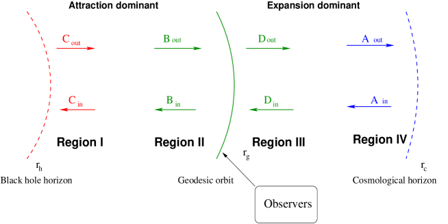
FIG. 1.: Configuration of Schwarzschild-de Sitter black holes: Observers are located at the two-spherical spacelike hypersurface where cosmological expansion and black hole attraction balance out exactly so that there is no acceleration on this hypersurface as like observers at Minkowski spacetimes, and as for a thermal radiation, observers will experience thermal temperatures $T_{\rm BH}$ and $T_{\rm DS}$ coming from two horizons.

We can divide our whole spacetimes into specific four regions as shown in the Fig. (1). With the assumption of $r_{h}<<r_{g}<<r_{c}$, as $r$ goes to the black hole horizon $r_{h}$, the SS black hole metric is prominent in the attraction dominant region (region (I) and (II)) in as

$$U(r)\approx 1-\frac{2M}{r},$$ (4)

while if we are in the expansion dominant region (region (III) and (IV)) which is accomplished by $r\rightarrow r_{c}>>r_{g}$, the metric (3) behaves as like a dS metric

$$U(r)\approx 1-\frac{\Lambda}{3}r^{2}.$$ (5)

Note that the metric element (3) is a patch of Eqs. (4) and (5) at the geodesic orbit $r_{g}$ but this picture is only valid for $r_{h}<<r_{g}<<r_{c}$. For each region, a field equation can be solved and the corresponding amplitudes of solutions between the four regions will be matched exactly. Then we define a reflection coefficient as a ratio between ingoing and outgoing fluxes in region (II) and region (III), and finally obtain the scattering amplitudes and thermal temperatures coming from these two horizons.

The dynamical behavior of a massive scalar field under the background (2) is described by

$$\left(\Box-m^{2}\right)\Psi(t,r,\theta,\phi)=0.$$ (6)

Using the separation of variables, $\Psi(t,r,\theta,\phi)=e^{-i\omega t}R(r)\Theta(\theta)e^{i\mu\phi}$, the field equation (6) becomes

$$\frac{1}{r^{2}}\partial_{r}\left(r^{2}U(r)\partial_{r}R(r)\right)+\left(\frac{\omega^{2}}{U(r)}-\frac{\nu(\nu+1)}{r^{2}}-m^{2}\right)R(r)=0,$$ (7)

$$\frac{1}{\sin\theta}\partial_{\theta}\left(\sin\theta\partial_{\theta}\Theta(\theta)\right)-\frac{\mu^{2}}{\sin^{2}\theta}\Theta(\theta)=-\nu(\nu+1)\Theta(\theta),$$ (8)

where $\nu$ is an angular mode.

III Low Energy Perturbation in the Black Hole Region

A Solution near the black holes(Region (I) and (II))

At first, let us consider the field equation (7) in the near black hole horizon region(Region (I) in Fig. (1)). As $r$ goes to $r_{h}$, the metric (2) becomes to be a SS metric, $U(r)\approx(1-2M/r)$. So the equation of motion (7) can be written as

$$\left(1-\frac{r_{h}}{r}\right)\partial_{r}^{2}R(r)+\left(\frac{2}{r}-\frac{r_{h}}{r^{2}}\right)\partial_{r}R(r)+\left(\frac{\omega^{2}}{\left(1-\frac{r_{h}}{r}\right)}-\frac{\nu(\nu+1)}{r^{2}}-m^{2}\right)R(r)=0,$$ (9)

where the horizon $r_{h}\approx 2M$ as $r\rightarrow r_{h}$. Taking a coordinate transformation such as $z=(r-r_{h})/r$, where $z$ spans from $0$ to $1$ as $r$ goes from $r_{h}$ to $r_{g}$, where we assumed that $r_{h}<<r_{g}$, the radial equation becomes

$$z(1-z)\partial_{z}^{2}R(z)+(1-z)\partial_{z}R(z)+\left(\frac{\omega^{2}r_{h}^{2}}{z}-\frac{\nu(\nu+1)}{1-z}-m^{2}r_{h}^{2}\right)R(z)=0.$$ (10)

Using $R(z)=z^{\alpha}(1-z)^{\beta}g(z)$ in order to remove two singular points at $z=0$ and $z=1$, Eq. (10) is written as

$$z(1-z)\partial_{z}^{2}g(z)+(1+2\alpha-(1+2\alpha+2\beta)z)\partial_{z}g(z)$$ (12)

$$+\frac{1}{z}(\alpha^{2}+\omega^{2}r_{h}^{2})g(z)+\frac{1}{1-z}(\beta^{2}-\beta-\nu(\nu+1))g(z)-((\alpha+\beta)^{2}+m^{2}r_{h}^{2})g(z)=0,$$

and we have $\alpha=\pm i\omega r_{h}$ and $\beta=\nu+1$. Then Eq. (12) becomes

$$z(1-z)\partial_{z}^{2}g(z)+(1+2\alpha-(1+2\alpha+2\beta)z)\partial_{z}g(z)-((\alpha+\beta)^{2}+m^{2}r_{h}^{2})g(z)=0.$$ (13)

Note that we take the plus signature of $\alpha$ since the solution will be symmetric for changing $\alpha$ into $-\alpha$. The solution of Eq. (13) is given as

$$R_{\rm(I)}(r)= C_{\rm out}z^{\alpha}(1-z)^{\beta}F(\alpha_{-}+\beta,\alpha_{+}+\beta,1+2\alpha;z)$$ (15)

$$\qquad+C_{\rm in}z^{-\alpha}(1-z)^{\beta}F(-\alpha_{+}+\beta,-\alpha_{-}+\beta,1-2\alpha;z),$$

where $\alpha_{\pm}=\alpha\pm imr_{h}=i(\omega\pm m)r_{h}$ and $C_{\rm in}$ and $C_{\rm out}$ are ingoing and outgoing coefficients, respectively.

Next, from the solution (15), we shall use a $z\rightarrow 1-z$ transformation [9],

$$F(a,b;a+b-l;z) = \frac{\Gamma(l)\Gamma(a+b-l)}{\Gamma(a)\Gamma(b)}(1-z)^{-l}\sum_{n=0}^{l-1}\frac{(a-l)_{n}(b-l)_{n}}{n!(1-l)_{n}}(1-z)^{n}$$ (16)

$$- \frac{(-1)^{l}\Gamma(a+b-l)}{\Gamma(a-l)\Gamma(b-l)}\sum_{n=0}^{\infty}\frac{(a)_{n}(b)_{n}}{n!(n+l)!}(1-z)^{n}$$ (17)

$$\times \left[\ln(1-z)-\psi(n+1)-\psi(n+l+1)+\psi(a+n)+\psi(b+n)\right],$$ (18)

where $\psi(z)$ is a digamma function and $a=\pm\alpha_{\mp}+\beta$, $b=\pm\alpha_{\pm}+\beta$, and $l=2\nu+1$ in our case. As $z\rightarrow 1$, for the lowest order of $n$, the solution (15) is transformed to the region (II) by using Eq. (16) as

$$R_{z\rightarrow 1}(r) = \left[C_{\rm out}\frac{\Gamma(2\beta-1)\Gamma(1+2\alpha)}{\Gamma(\alpha_{-}+\beta)\Gamma(\alpha_{+}+\beta)}+C_{\rm in}\frac{\Gamma(2\beta-1)\Gamma(1-2\alpha)}{\Gamma(-\alpha_{+}+\beta)\Gamma(-\alpha_{-}+\beta)}\right]\left(\frac{r_{h}}{r}\right)^{1-\beta}$$ (19)

$$+ \left[C_{\rm out}\frac{{\cal D}_{\nu}^{\rm out}\Gamma(1+2\alpha)}{\Gamma(1+\alpha_{-}-\beta)\Gamma(1+\alpha_{+}-\beta)}+C_{\rm in}\frac{{\cal D}_{\nu}^{\rm in}\Gamma(1-2\alpha)}{\Gamma(1-\alpha_{+}-\beta)\Gamma(1-\alpha_{-}-\beta)}\right]\left(\frac{r_{h}}{r}\right)^{\beta},$$ (20)

where ${\cal D}_{\nu}^{\rm in}=-\psi(1)-\psi(2\beta)+\psi(-\alpha_{+}+\beta)+\psi(-\alpha_{-}+\beta)={\cal D}_{\nu}^{\ast\rm out}$ and note that Eq. (19) is symmetric for changing $\beta$ into $1-\beta$.

B Asymptotic solution at Region (II)

We now consider the asymptotic limit of $r\rightarrow r_{g}>>r_{h}$ which describes the region (II) in Fig. (1). In this limit, the field equation (9) becomes

$$\partial_{r}^{2}R(r)+\frac{2}{r}\partial_{r}R(r)+\left(p^{2}-\frac{\nu(\nu+1)}{r^{2}}\right)R(r)=0,$$ (21)

where $p=\sqrt{\omega^{2}-m^{2}}$, and the solution is given as Bessel functions,

$$R_{r_{g}}^{(z)}(r)=\frac{B_{1}}{\sqrt{r}}J_{-\frac{1}{2}(1-2\beta)}(pr)+\frac{B_{2}}{\sqrt{r}}J_{\frac{1}{2}(1-2\beta)}(pr),$$ (22)

where $B_{1}$ and $B_{2}$ are amplitudes of the solution. The solution (22) can be expanded by keeping the lowest leading order of $r$ and defining new coefficients $B_{\rm in}$ and $B_{\rm out}$ as

$$B_{1}=B_{\rm in}+B_{\rm out}$$ (23)

$$B_{2}=i(B_{\rm in}-B_{\rm out}),$$ (24)

in order to separate wave modes into in-and out-going parts, the solution is written as

$$R_{r_{g}}^{(z)}(r)=B_{\rm in}\left(\Omega_{\beta}^{(+)}\frac{1}{r^{1-\beta}}+i\Omega_{\beta}^{(-)}\frac{1}{r^{\beta}}\right)+B_{\rm out}\left(\Omega_{\beta}^{(+)}\frac{1}{r^{1-\beta}}-i\Omega_{\beta}^{(-)}\frac{1}{r^{\beta}}\right),$$ (25)

where $\Omega_{\beta}^{(+)}\equiv\left(\frac{1}{2}p\right)^{-\frac{1}{2}(1-2\beta)}/{\Gamma\left(\frac{1}{2}+\beta\right)}$ and $\Omega_{\beta}^{(-)}\equiv\left(\frac{1}{2}p\right)^{\frac{1}{2}(1-2\beta)}/{\Gamma\left(\frac{3}{2}-\beta\right)}$. Note that $\Omega_{\beta}^{(\pm)\ast}=\Omega_{\beta}^{(\pm)}$ and $\Omega_{\beta}^{(+)}\Omega_{\beta}^{(-)}$ is explicitly calculated as $(\Omega_{\beta}^{(+)}\Omega_{\beta}^{(-)})=\frac{2\cos\beta\pi}{\pi(1-2\beta)}=\frac{2(-1)^{\beta}}{\pi(1-2\beta)}$.

C Matching process and temperature

As easily seen from Eqs. (19) and (25), by matching these solutions, we obtain the following relations,

$$B_{\rm in} = \frac{1}{2}\left[\frac{r_{h}^{1-\beta}}{\Omega_{\beta}^{(+)}}\left(C_{\rm in}\frac{\Gamma(2\beta-1)\Gamma(1-2\alpha)}{\Gamma(-\alpha_{+}+\beta)\Gamma(-\alpha_{-}+\beta)}+C_{\rm out}\frac{\Gamma(2\beta-1)\Gamma(1+2\alpha)}{\Gamma(\alpha_{-}+\beta)\Gamma(\alpha_{+}+\beta)}\right)\right.$$ (26)

$$- \left.i\frac{r_{h}^{\beta}}{\Omega_{\beta}^{(-)}}\left(C_{\rm in}\frac{\Gamma(1-2\alpha){\cal D}_{\nu}^{\rm in}}{\Gamma(1-\alpha_{+}-\beta)\Gamma(1-\alpha_{-}-\beta)}+C_{\rm out}\frac{\Gamma(1+2\alpha){\cal D}_{\nu}^{\rm out}}{\Gamma(1+\alpha_{+}-\beta)\Gamma(1+\alpha_{-}-\beta)}\right)\right],$$ (27)

$$B_{\rm out} = \frac{1}{2}\left[\frac{r_{h}^{1-\beta}}{\Omega_{\beta}^{(+)}}\left(C_{\rm in}\frac{\Gamma(2\beta-1)\Gamma(1-2\alpha)}{\Gamma(-\alpha_{+}+\beta)\Gamma(-\alpha_{-}+\beta)}+C_{\rm out}\frac{\Gamma(2\beta-1)\Gamma(1+2\alpha)}{\Gamma(\alpha_{-}+\beta)\Gamma(\alpha_{+}+\beta)}\right)\right.$$ (28)

$$+ \left.i\frac{r_{h}^{\beta}}{\Omega_{\beta}^{(-)}}\left(C_{\rm in}\frac{\Gamma(1-2\alpha){\cal D}_{\nu}^{\rm in}}{\Gamma(1-\alpha_{+}-\beta)\Gamma(1-\alpha_{-}-\beta)}+C_{\rm out}\frac{\Gamma(1+2\alpha){\cal D}_{\nu}^{\rm out}}{\Gamma(1+\alpha_{+}-\beta)\Gamma(1+\alpha_{-}-\beta)}\right)\right].$$ (29)

At this stage, we impose a boundary condition $C_{\rm out}=0$, which implies that there are no outgoing modes of scalar fields since all modes of fields are absorbed into the black hole horizon. Defining a flux as

$${\cal F}=\frac{2\pi}{i}U(r)\left(R^{\ast}(r)\partial_{r}R(r)-R(r)\partial_{r}R^{\ast}(r)\right),$$ (30)

we obtain them near the geodesic orbit $r_{g}$ as

$${\cal F}_{r_{g}}^{\rm out}=-8|B_{\rm out}|^{2}(-1)^{\beta}r_{g}^{-2},$$ (31)

$${\cal F}_{r_{g}}^{\rm in}=8|B_{\rm in}|^{2}(-1)^{\beta}r_{g}^{-2}.$$ (32)

The reflection coefficient near the geodesic orbit $r_{g}$ is defined as a ratio between ingoing and outgoing fluxes, and consequently it gives

$${\cal R_{\rm BH}}=\left|\frac{{\cal F}_{r_{g}}^{\rm in}}{{\cal F}_{r_{g}}^{\rm out}}\right|^{2}=\left|\frac{B_{\rm in}}{B_{\rm out}}\right|^{2}.$$ (33)

Furthermore, statistical-thermodynamic temperature is defined as a vacuum expectation value of a number operator $N$ and it is related to the reflection coefficient [10, 11],

$$<0|N|0>=\frac{1}{e^{{\omega}/{T_{stat}}}-1}=\frac{{\cal R}_{\rm BH}}{1-{\cal R}_{\rm BH}}.$$ (34)

Therefore, we have a thermal temperature of black holes,

$$T_{stat}=-\frac{\omega}{\ln{\cal R}_{\rm BH}}.$$ (35)

From Eq. (26) with the boundary condition $C_{\rm out}=0$, the logarithm term in Eq. (35) becomes

$$\ln{\cal R}_{\rm BH}=\ln\left(\frac{1-i\xi}{1+i\xi}\right)=-2i\xi+{\cal O}(\xi^{2}),$$ (36)

where

$$\xi \equiv \frac{1}{2\pi}r_{h}(-1)^{\beta+1}\Gamma(2\beta)\sin\pi\alpha_{+}\sin\pi\alpha_{-}({\cal D}_{\nu}^{in}-{\cal D}_{\nu}^{\ast in})$$ (37)

$$\times \left(\frac{r_{h}^{2-2\beta}(\frac{1}{2}p)^{1-2\beta}\Gamma^{2}\left(\beta+\frac{1}{2}\right)\Gamma^{2}(2\beta-1)}{\Gamma(\alpha_{+}+\beta)\Gamma(-\alpha_{+}+\beta)\Gamma(\alpha_{-}+\beta)\Gamma(-\alpha_{-}+\beta)}\right.$$ (38)

$$+ \left.\frac{r_{h}^{2\beta}(\frac{1}{2}p)^{2\beta-1}\Gamma^{2}\left(\frac{3}{2}-\beta\right)|{\cal D}_{\nu}^{\rm in}|^{2}}{\Gamma(1+\alpha_{+}-\beta)\Gamma(1+\alpha_{-}-\beta)\Gamma(1-\alpha_{+}-\beta)\Gamma(1-\alpha_{-}-\beta)}\right)^{-1}.$$ (39)

For simplicity, considering the main contribution of $s$-modes(vanishing angular potential) when $\beta=1$ as shown in Ref. [7, 12], Eq. (37) is simplified as $\xi=-\pi^{2}i\omega r_{h}/3$ by using the Schwarz’s inequality. So, we obtain the “minimal” thermal temperature,

$$T_{stat}^{\rm min}=T_{\rm BH}=\frac{1}{2\pi r_{h}}\left(\frac{3}{\pi}\right)\approx\frac{1}{2\pi r_{h}},$$ (40)

where it agrees with the well-known Hawking temperature for the SS black hole. Therefore, we have shown that the desired Hawking temperature can be reproduced as a “minimal” statistical temperature in attraction dominant region (Region (I) and (II)).

IV Low Energy Perturbation in the De-Sitter Region

A Solution near the de Sitter Spacetimes (Region (III) and (IV))

Now we study the solution in the expansion dominant region (region (III) and (IV)). As $r\rightarrow r_{c}$, Eq. (7) becomes

$$\left(r_{c}^{2}-r^{2}\right)\partial_{r}^{2}R(r)+\left(\frac{2}{r}-\frac{4r}{r_{c}^{2}}\right)\partial_{r}R(r)+\left(\frac{\omega^{2}r_{c}^{2}}{(r_{c}^{2}-r^{2})}-\frac{\nu(\nu+1)}{r^{2}}-m^{2}\right)R(r)=0,$$ (41)

where $r_{c}$ is nearly $(3\Lambda^{-1})^{1/2}$ as $r$ goes to $r_{c}$. By choosing a coordinate as $y=1-r^{2}/r_{c}^{2}$ where $y$ spans from $0$ to $1$, the radial equation (41) is written as

$$y(1-y)\partial_{y}^{2}R(y)+\frac{1}{2}(2-5y)\partial_{y}R(y)+\left(\frac{\omega^{2}r_{c}^{2}}{4y}-\frac{\nu(\nu+1)}{4(1-y)}-\frac{m^{2}r_{c}^{2}}{4}\right)R(y)=0.$$ (42)

Singular points at $y=0$ and $y=1$ can be eliminated by choosing $R(y)=y^{\tilde{\alpha}}(1-y)^{\tilde{\beta}}u(y)$, and Eq. (42) is written as

$$y(1-y)\partial_{y}^{2}u(y)+\left(1+2{\tilde{\alpha}}-\frac{1}{2}\left(4{\tilde{\alpha}}+4{\tilde{\beta}}+5\right)y\right)\partial_{y}u(y)$$ (43)

$$\qquad\qquad\qquad\qquad+\frac{1}{y}\left({\tilde{\alpha}}^{2}+\frac{\omega^{2}r_{c}^{2}}{4}\right)u(y)+\frac{1}{1-y}\left({\tilde{\beta}}^{2}+\frac{{\tilde{\beta}}}{2}-\frac{\nu(\nu+1)}{4}\right)$$ (44)

$$\qquad\qquad\qquad\qquad\qquad\qquad\qquad\qquad-\left[({\tilde{\alpha}}+{\tilde{\beta}})({\tilde{\alpha}}+{\tilde{\beta}}+\frac{3}{2})+\frac{m^{2}r_{c}^{2}}{4}\right]u(y)=0.$$ (45)

Determining ${\tilde{\alpha}}=i\omega r_{c}/2$ and ${\tilde{\beta}}=\nu/2=-(1-\beta)/2$, Eq. (43) becomes

$$y(1-y)\partial_{y}^{2}u(y)+\left(1+2{\tilde{\alpha}}-\frac{1}{2}\left(4{\tilde{\alpha}}+4{\tilde{\beta}}+5\right)y\right)\partial_{y}u(y)$$ (46)

$$\qquad\qquad\qquad\qquad\qquad\qquad\qquad\qquad-\left[({\tilde{\alpha}}+{\tilde{\beta}})({\tilde{\alpha}}+{\tilde{\beta}}+\frac{3}{2})+\frac{m^{2}r_{c}^{2}}{4}\right]u(y)=0.$$ (47)

By defining $\gamma_{\pm}\equiv(3\pm\sqrt{9-4m^{2}r_{c}^{2}})/4$, the solution is given as

$$R(y) = A_{\rm in}y^{\tilde{\alpha}}(1-y)^{\tilde{\beta}}F(\gamma_{-}+{\tilde{\alpha}}+{\tilde{\beta}},\gamma_{+}+{\tilde{\alpha}}+{\tilde{\beta}},1+2{\tilde{\alpha}};y)$$ (49)

$$\qquad\qquad+A_{\rm out}y^{-\tilde{\alpha}}(1-y)^{\tilde{\beta}}F(\gamma_{-}-{\tilde{\alpha}}+{\tilde{\beta}},\gamma_{+}-{\tilde{\alpha}}+{\tilde{\beta}},1-2{\tilde{\alpha}};y),$$

where $\gamma_{+}+\gamma_{-}=3/2$. Note that the solution (49) follows a $z\rightarrow 1-z$ transformation given by

$$F(a,b,c;z) = \frac{\Gamma(a)\Gamma(c-a-b)}{\Gamma(c-a)\Gamma(c-b)}F(a,b,a+b-c+1;1-z)$$ (50)

$$+ (1-z)^{c-a-b}\frac{\Gamma(c)\Gamma(a+b-c)}{\Gamma(a)\Gamma(b)}F(c-a,c-b,c-a-b+1;1-z).$$ (51)

Therefore, for the limit of $y\rightarrow 1$ ($r\rightarrow r_{g}<<r_{c}$), we obtain the solution in region (III) of Eq.(49),

$$R_{y\rightarrow 1}(r)$$ (52)

$$= \left(\frac{A_{\rm in}\Gamma(1+2{\tilde{\alpha}})\Gamma\left(-2{\tilde{\beta}}-\frac{1}{2}\right)}{\Gamma(1+{\tilde{\alpha}}-{\tilde{\beta}}-\gamma_{-})\Gamma(1+{\tilde{\alpha}}-{\tilde{\beta}}-\gamma_{+})}+\frac{A_{\rm out}\Gamma(1-2{\tilde{\alpha}})\Gamma\left(-2{\tilde{\beta}}-\frac{1}{2}\right)}{\Gamma(1-{\tilde{\alpha}}-{\tilde{\beta}}-\gamma_{-})\Gamma(1-{\tilde{\alpha}}-{\tilde{\beta}}-\gamma_{+})}\right)\left(\frac{r_{c}}{r}\right)^{1-\beta}$$ (53)

$$+ \left(\frac{A_{\rm in}\Gamma(1+2{\tilde{\alpha}})\Gamma\left(2{\tilde{\beta}}+\frac{1}{2}\right)}{\Gamma({\tilde{\alpha}}+{\tilde{\beta}}+\gamma_{-})\Gamma({\tilde{\alpha}}+{\tilde{\beta}}+\gamma_{+})}+\frac{A_{\rm out}\Gamma(1-2{\tilde{\alpha}})\Gamma\left(2{\tilde{\beta}}+\frac{1}{2}\right)}{\Gamma(-{\tilde{\alpha}}+{\tilde{\beta}}+\gamma_{-})\Gamma(-{\tilde{\alpha}}+{\tilde{\beta}}+\gamma_{+})}\right)\left(\frac{r_{c}}{r}\right)^{\beta}.$$ (54)

B Asymptotic solution at region (III)

On the other hand, for the asymptotic limit $r\rightarrow r_{g}$, the equation of motion (46) can be written as the same form with Eq. (21) and the solution is given by Bessel functions with different amplitudes, $D_{1}$ and $D_{2}$,

$$R_{r_{g}}^{(y)}(r)=\frac{D_{1}}{\sqrt{r}}J_{-\frac{1}{2}(1-2\beta)}(pr)+\frac{D_{2}}{\sqrt{r}}J_{\frac{1}{2}(1-2\beta)}(pr),$$ (55)

where $p=\sqrt{\omega^{2}-m^{2}}$ and $\beta=\nu+1$. In the same way for the previous calculation, by defining new coefficients $D_{\rm in}$ and $D_{\rm out}$ as

$$D_{1}=D_{\rm in}+D_{\rm out}$$ (57)

$$D_{2}=i(D_{\rm in}-D_{\rm out}),$$

the solution (55) can be written as

$$R_{r_{g}}^{(y)}(r)=D_{\rm in}\left(\Omega_{\beta}^{(+)}\frac{1}{r^{1-\beta}}+i\Omega_{\beta}^{(-)}\frac{1}{r^{\beta}}\right)+D_{\rm out}\left(\Omega_{\beta}^{(+)}\frac{1}{r^{1-\beta}}-i\Omega_{\beta}^{(-)}\frac{1}{r^{\beta}}\right).$$ (58)

C Matching process and temperature

Comparing Eq. (52) with Eq. (58) to perform a coefficient match, we obtain the relations between coefficients at region (III) and (IV),

$$D_{\rm in} = \frac{1}{2\Omega_{\beta}^{(+)}}\left(\frac{A_{\rm in}r_{c}^{\beta-1}\Gamma(1+2{\tilde{\alpha}})\Gamma(-2{\tilde{\beta}}-\frac{1}{2})}{\Gamma(1+{\tilde{\alpha}}-{\tilde{\beta}}-\gamma_{-})\Gamma(1+{\tilde{\alpha}}-{\tilde{\beta}}-\gamma_{+})}+\frac{A_{\rm out}r_{c}^{\beta-1}\Gamma(1-2{\tilde{\alpha}})\Gamma(-2{\tilde{\beta}}-\frac{1}{2})}{\Gamma(1-{\tilde{\alpha}}-{\tilde{\beta}}-\gamma_{-})\Gamma(1-{\tilde{\alpha}}-{\tilde{\beta}}-\gamma_{+})}\right)$$ (59)

$$- i\frac{1}{2\Omega_{\beta}^{(-)}}\left(\frac{A_{\rm in}r_{c}^{-\beta}\Gamma(1+2{\tilde{\alpha}})\Gamma(2{\tilde{\beta}}+\frac{1}{2})}{\Gamma({\tilde{\alpha}}+{\tilde{\beta}}+\gamma_{-})\Gamma({\tilde{\alpha}}+{\tilde{\beta}}+\gamma_{+})}+\frac{A_{\rm out}r_{c}^{-\beta}\Gamma(1-2{\tilde{\alpha}})\Gamma(2{\tilde{\beta}}+\frac{1}{2})}{\Gamma(-{\tilde{\alpha}}+{\tilde{\beta}}+\gamma_{-})\Gamma(-{\tilde{\alpha}}+{\tilde{\beta}}+\gamma_{+})}\right)$$ (60)

$$D_{\rm out} = \frac{1}{2\Omega_{\beta}^{(+)}}\left(\frac{A_{\rm in}r_{c}^{\beta-1}\Gamma(1+2{\tilde{\alpha}})\Gamma(-2{\tilde{\beta}}-\frac{1}{2})}{\Gamma(1+{\tilde{\alpha}}-{\tilde{\beta}}-\gamma_{-})\Gamma(1+{\tilde{\alpha}}-{\tilde{\beta}}-\gamma_{+})}+\frac{A_{\rm out}r_{c}^{\beta-1}\Gamma(1-2{\tilde{\alpha}})\Gamma(-2{\tilde{\beta}}-\frac{1}{2})}{\Gamma(1-{\tilde{\alpha}}-{\tilde{\beta}}-\gamma_{-})\Gamma(1-{\tilde{\alpha}}-{\tilde{\beta}}-\gamma_{+})}\right)$$ (61)

$$+ i\frac{1}{2\Omega_{\beta}^{(-)}}\left(\frac{A_{\rm in}r_{c}^{-\beta}\Gamma(1+2{\tilde{\alpha}})\Gamma(2{\tilde{\beta}}+\frac{1}{2})}{\Gamma({\tilde{\alpha}}+{\tilde{\beta}}+\gamma_{-})\Gamma({\tilde{\alpha}}+{\tilde{\beta}}+\gamma_{+})}+\frac{A_{\rm out}r_{c}^{-\beta}\Gamma(1-2{\tilde{\alpha}})\Gamma(2{\tilde{\beta}}+\frac{1}{2})}{\Gamma(-{\tilde{\alpha}}+{\tilde{\beta}}+\gamma_{-})\Gamma(-{\tilde{\alpha}}+{\tilde{\beta}}+\gamma_{+})}\right).$$ (62)

Now we impose a boundary condition $A_{\rm out}=0$, which means that there are no wave modes falling into the cosmological horizon, and we define a reflection coefficient at the geodesic orbit $r_{g}$ as

$${\cal R}_{\rm DS}=\left|\frac{\tilde{\cal F}_{\rm out}}{\tilde{\cal F}_{\rm in}}\right|=\left|\frac{D_{\rm out}}{D_{\rm in}}\right|^{2},$$ (63)

where the ingoing and outgoing fluxes at $r_{g}$ are obtained by the definition (30),

$$\tilde{\cal F}_{r_{g}}^{\rm in}=8|D_{\rm in}|^{2}(-1)^{\beta}r_{g}^{-2}$$ (64)

$$\tilde{\cal F}_{r_{g}}^{\rm out}=-8|D_{\rm out}|^{2}(-1)^{\beta}r_{g}^{-2}.$$ (65)

With the help of Eq. (59), the reflection coefficient (63) is written as

$${\cal R}_{\rm DS}=\frac{1+i{\tilde{\xi}}}{1-i{\tilde{\xi}}},$$ (66)

where

$${\tilde{\xi}} \equiv r_{c}\sin 2{\tilde{\alpha}}\pi\sin^{2}\frac{\pi\beta}{2}$$ (67)

$$\times \left(\frac{\pi^{2}r_{c}^{2(1-\beta)}(\frac{1}{2}p)^{1-2\beta}}{\Gamma(1-{\tilde{\alpha}}-{\tilde{\beta}}-\gamma_{-})\Gamma(1+{\tilde{\alpha}}-{\tilde{\beta}}-\gamma_{-})\Gamma(1-{\tilde{\alpha}}-{\tilde{\beta}}-\gamma_{+})\Gamma(1+{\tilde{\alpha}}-{\tilde{\beta}}-\gamma_{+})}\right.$$ (68)

$$+ \left.\frac{r_{c}^{2\beta}\pi^{2}(\frac{1}{2}p)^{-(1-2\beta)}}{\Gamma(\gamma_{-}-{\tilde{\alpha}}+{\tilde{\beta}})\Gamma(\gamma_{-}+{\tilde{\alpha}}+{\tilde{\beta}})\Gamma(\gamma_{+}-{\tilde{\alpha}}+{\tilde{\beta}})\Gamma(\gamma_{+}+{\tilde{\alpha}}+{\tilde{\beta}})}\right)^{-1}.$$ (69)

By using the relations ${\tilde{\beta}}=-(1-\beta)/2$ and $\Gamma(s)\Gamma(1-s)={\pi}/{\sin\pi s}$, and the thermal temperature is given as,

$$T_{stat}=-\frac{\omega}{\ln{\cal R}_{\rm DS}}\approx-\frac{\omega}{2i{\tilde{\xi}}}$$ (70)

in a leading order of $\omega$. To be explicit, for $\nu=0$, i.e. ${\tilde{\beta}}=0$, Eq. (67) is simplified as

$${\tilde{\xi}}=\frac{\sin 2\pi{\tilde{\alpha}}}{\sqrt{\cos^{2}\pi(\gamma_{+}-\gamma_{-})-\sin^{2}2\pi{\tilde{\alpha}}}}.$$ (71)

Expanding Eq. (71) in a low energy limit, ${\tilde{\xi}}=2\pi{\tilde{\alpha}}+{\cal O}(m^{2},{\tilde{\alpha}}^{2})$ and the “minimal” thermal temperature can be obtained as

$$T_{stat}^{min}=T_{\rm DS}\approx\frac{1}{2\pi r_{c}},$$ (72)

which agrees with the thermal temperature of the dS spacetimes.

V Discussions

In summary, we have studied the scattering problem of the massive scalar field on the SSdS background by assuming the low energy of the probing field. For the small static SSdS black hole, the whole spacetimes can be considered as a patch of two different regions (SS black hole and dS spacetimes) and the geodesic orbit where the black hole attraction and cosmic expansion balance out is introduced. Using the low energy approximation, the corresponding statistical temperatures from two horizons are derived, and it is interesting to note that the minimal bounds of these temperatures are equivalent to the thermal temperatures obtained from the metric.

As a comment, we should perform a fine-tuning process between the wave functions at the region (II) and (III) in Sec. II. The wave functions of the massive scalar field should be connected smoothly at the geodesic orbit since it is regarded as a continuous function in the whole regions. Therefore, from Eqs. (25) and (58), we define $B_{\rm in}\equiv N_{\rm in}D_{\rm in}$ and $B_{\rm out}\equiv N_{\rm out}D_{\rm out}$, respectively, where $N_{\rm in}$ and $N_{\rm out}$ are proportional constants. And then, Eqs. (33) and (63) produce a relation $R_{\rm DS}R_{\rm BH}=|{\cal Q}|^{-2}$ by defining $|{\cal Q}|^{2}=|N_{\rm in}|^{2}/|N_{\rm out}|^{2}$ and it determines,

$$|{\cal Q}|^{2}=e^{\omega\left(T_{BH}^{-1}+T_{DS}^{-1}\right)},$$ (73)

which is a fine-tuning for mismatched wave functions at the geodesic orbit and it correlates the cosmological horizon $r_{c}$ with the black hole horizon $r_{h}$. By means of this final coefficient-tuning, the wave functions of probing fields are continuous and connected smoothly in the whole area.

Now let us discuss about the qualitative behaviors of non-degenerate and nearly degenerate cases of SSdS black holes. As mentioned above, our whole calculations have been done by assuming that the black hole horizon size is much smaller than that of the cosmological horizon, which describes a small SSdS black hole. Since the black hole will be hotter than the cosmological horizon, the one will evaporate faster than the other, and the black hole horizon will disappear at the end of evaporation. And then the SSdS spacetimes may become the pure dS spacetimes at the end of the evaporation. At this stage, one may ask a question : “After evaporation at final stage, is it really possible to transit from the SSdS spacetimes to the dS ones?” In fact, to answer this question explicitly, one should study this model with the gravitational back reaction by using the time evolution of the small SSdS black hole, however we do not discuss anymore because of complexity of this analysis.

On the other hand, we naturally consider the degenerate case of horizons that the black hole horizon is equal to the cosmological horizon. In this case, we expect that the black hole will be in the thermal equilibrium state since the black hole and cosmological horizons have the same surface gravity. Therefore, when the black hole horizon ($r_{h}$) approaches to the cosmological horizon ($r_{c}$), the two $S^{2}$ hypersufaces ($r_{h}$ and $r_{c}$) meet each other in a hypersurface ($r_{g}$), and this is somewhat trivial to discuss. To investigate the small perturbation from the thermal equilibrium, we can consider the nearly degenerate case whose metric is given by

$$(ds)^{2}=-\frac{1}{\sqrt{\Lambda}}\left(1+\frac{2}{3}\delta{\rm cos}R\right){\rm sin}^{2}Rd^{2}T+\frac{1}{\Lambda}\left(1-\frac{2}{3}\delta{\rm cos}R\right)d^{2}R+\frac{1}{\Lambda}\left(1-2\delta{\rm cos}\right)d^{2}\Omega_{(2)}$$ (74)

with defining new time and radial coordinates $T$ and $R$ by

$$t = \frac{1}{\delta\sqrt{\Lambda}}T,$$ (75)

$$r = \frac{1}{\sqrt{\Lambda}}\left(1-\delta{\rm cos}R-\frac{1}{6}\delta^{2}\right),$$ (76)

and $9M^{2}\Lambda=1-3\delta^{2}$, where $0\leq\delta\leq 1$. And the temperatures from two horizons are given by Ref. [2]

$$T_{{\rm h,c}}=\frac{1}{2\pi}\sqrt{\Lambda}\left(1\pm\frac{2}{3}\delta\right)+O(\delta^{2}),$$ (77)

where the upper (lower) sign is for the black hole (cosmological) horizon. Note that if $\delta$ goes to zero, Eq. (77) describes the degenerate temperature characterized by only a cosmological constant $\Lambda$, and the instability of the nearly degenerate SSdS black hole has been studied by adding the one loop quantum correction terms [3]. As a further work, if the scattering problem in the nearly degenerate SSdS black hole background is solved by use of the low energy perturbation method, the results of both temperatures will be compatible with Eq. (77).

Acknowledgments
This work has been achieved partially for participating in the APCTP-PIMS Summer Workshop at SFU, Canada. W. T. Kim and J. J. Oh would like to thank PIMS for hospitality during staying at SFU. J. J. Oh and K. H. Yee would like to thank V. P. Frolov for helpful comments while they were participating in the 6th APCTP Winter School at POSTECH, Korea. This work was supported by the Korea Research Foundation Grant, KRF-2001-015-DP0083.

REFERENCES

- [1] S. Perlmutter et al, Measurements of the Cosmological Parameters and from the First 7 Supernovae at , Astrophys. J. 483, 565 (1997) , [astro-ph/9608192]; S. Perlmutter, Supernovae, dark energy, and the accelerating universe: The status of the cosmological parameters, in Proc. of the 19th Int. Sym. on Photon and Lepton Interactions at High Energy LP99, Int. J. Mod. Phys. A15S1, 715 (2000).
- [2] R. Bousso and S. W. Hawking, Pair creation of black holes during inflation, Phys. Rev. D54, 6312 (1996).
- [3] R. Bousso and S. W. Hawking, (Anti-)evaporation of Schwarzschild-de Sitter black holes, Phys. Rev. D57, 2436 (1998).
- [4] G. W. Gibbons and S. W. Hawking, Action Integrals and Partition Functions in Quantum Gravity, Phys. Rev. D15, 2752 (1977).
- [5] P. Ginsparg and M. J. Perry, Semiclassical Perdurance of De Sitter Space, Nucl. Phys. B222, 245 (1983).
- [6] J. Maldacena and A. Strominger, Universal low-energy dynamics for rotating black holes, Phys. Rev. D56, 4975 (1997).
- [7] M. Cveti and F. Larsen, Greybody factors for black holes in four dimensions : Particles with spin, Phys. Rev. D57, 6297 (1998).
- [8] H. Suzuki, E. Takasugi, and H. Umetsu, Absorption rate of the Kerr-de Sitter black hole and the Kerr-Newman-de Sitter black hole, Prog. Theor. Phys. 103, 723 (2000) ; Analytic Solutions of Teukolsky Equation in Kerr-de Sitter and Kerr-Newman-de Sitter Geometries, Prog. Theor. Phys. 102, 253 (1999).
- [9] M. Abramowitz and I. A. Stegun, Handbook of Mathematical Functions, Dover Publication Inc., New York, ninth printing, (1970).
- [10] W. T. Kim and J. J. Oh, Dilaton driven Hawking radiation in AdS2 black hole, Phys. Lett. B461, 189 (1999).
- [11] K. Ghoroku and A. L. Larsen, Hawking temperature and string scattering off the 2+1 black hole, Phys. Lett. B328, 28 (1994).
- [12] V. P. Frolov, in private communication for participating in “6th APCTP Winter School on Black Hole Astrophysics 2002” at POSTECH, Korea.